Naturally Heavy Scalars in
Supersymmetric Grand Unified Theories

Abstract

The supersymmetric flavor, $CP$ and Polonyi problems are hints that the fundamental scale of the soft supersymmetry breaking parameters may be above a TeV, in apparent conflict with naturalness. We consider the possibility that multi-TeV scalar masses are generated by Planck- or unification-scale physics, and find the conditions under which the masses of scalars with large Yukawa couplings are driven, radiatively and asymptotically, to the weak scale through renormalization group evolution. Light third generation scalars then satisfy naturalness, while first and second generation scalars remain heavy to satisfy experimental constraints. We find that this mechanism is beautifully realized in the context of grand unified theories. In particular, the existence of right-handed neutrinos plays an important role in allowing remarkably simple scenarios. For example, for SO(10) boundary conditions with the squared masses of Higgs scalars double those of sleptons and squarks, we find that the entire scalar mass scale may be increased to 4 TeV at the unification scale without sacrificing naturalness.

I Introduction

The Achilles heel of supersymmetry lies, arguably, in the difficulty of satisfying naturalness while simultaneously decoupling supersymmetric effects from low-energy experimental observables. Naturalness is typically taken to require supersymmetric particle masses below $\sqrt{(4\pi/\alpha)}M_{W}\sim 1\text{ TeV}$, a few times the weak scale. In contrast, without an understanding of small scalar mass splittings, mixing angles, and $CP$-violating phases, a variety of experimental measurements suggest that supersymmetric scalar masses must lie well above a TeV.

The experimental constraints have varying degrees of significance and model dependence. Examples include the following:

• The kaon system. Constraints from the $K$ system depend on the flavor and chirality structure of the scalar quarks. Roughly speaking, however, for moderate degeneracies, the constraint from $\epsilon_{K}$ is most severe; it requires squark masses of order 100 TeV. Likewise, the $K-\bar{K}$ mass splitting needs squark masses of order 10 TeV. (See Ref. [1] for details.)

• Electric dipole moments. The electric dipole moments of the neutron and electron typically require multi-TeV squark and slepton masses if the relevant phases are not suppressed [2]. EDMs are flavor-conserving and so cannot be suppressed by scalar degeneracy; for example, they imply severe constraints on scalar masses (or phases) even in models with gauge-mediated supersymmetry breaking. [3].

• The proton lifetime. Lower bounds on the proton lifetime place strong constraints on supersymmetric grand unified theories (GUTs), especially for large $\tan\beta$ [4]. The predicted decay rates depend on the (super)heavy and the light supersymmetric particle spectra; they are greatly suppressed for multi-TeV scalar masses.

• The Polonyi problem. Many supersymmetric theories contain late decaying scalar fields that ruin the successful predictions of Big Bang nucleosynthesis [5]. This problem is independent of scalar degeneracies or phases, but may be solved if the scale of supersymmetry breaking is of order 10 TeV [6].

In addition, many models predict scalar masses hierarchically larger than gaugino masses [7]. Given the current bounds on gaugino masses, scalar masses must then be well above a TeV.

The conflict between naturalness and experimental constraints may be resolved by observing that, roughly speaking, naturalness restricts the masses of scalars with large Yukawa couplings, while experiment constrains the masses of scalars with small Yukawas [8]. Naturalness affects particles that are strongly coupled to the Higgs sector, while experimental constraints are strongest in sectors with light fermions that are plentifully produced. This suggests that naturalness and experimental constraints may be simultaneously satisfied by an “inverted hierarchy” approach, in which light fermions have heavy superpartners, and vice versa. In particular, third generation scalars with masses $m_{\rm light}\lesssim 1\text{ TeV}$ satisfy naturalness constraints, while first and second generation scalars at some much higher scale $m_{\rm heavy}$ avoid many experimental difficulties. A number of possibilities have been proposed to dynamically generate scalar masses at two hierarchically separated scales [9, 10, 11].

In this paper, we shall investigate a new mechanism for generating an inverted hierarchy. We will assume that all scalar masses are of order $m_{\rm heavy}$ when produced at some scale, say the GUT or Planck scale. We will then use renormalization group evolution to create an inverted hierarchy at the weak scale. This mechanism works because the renormalization group equations automatically suppress the masses of scalars associated with fermions which have large Yukawa couplings. The masses of these scalars (and only these scalars) are driven to $m_{\rm light}$. This mechanism was investigated recently in models with large top and bottom Yukawa couplings (and all others small) [12]. It was shown that, for particular high scale boundary conditions, all scalars with large Yukawas may be driven asymptotically to $m_{\rm light}$ in the infrared. Stops, sbottoms, and Higgs scalars are then naturally light at the weak scale, while the masses of all other scalars remain heavy. In this way a very large hierarchy can be created dynamically.

In what follows we will consider the well-motivated supersymmetric GUTs, with special emphasis on SO(10) unified theories. As is well-known, such theories, among other merits, successfully predict gauge coupling unification and naturally accommodate massive neutrinos. In the present context, however, they have even more virtues. First, they naturally provide the universal and large third generation Yukawa couplings required to implement the inverted hierarchy. Second, as we will see, the existence of a right-handed neutrino plays an important part in creating a plausible fixed point structure. These virtues make grand unified theories the natural setting for the radiatively generated inverted hierarchy mechanism.

We will begin in Sec. II with a discussion of the fixed point structure of the scalar mass renormalization group equations (RGEs). In Sec. III we will analyze the inverted hierarchy in grand unified models with right-handed neutrinos. Finally, in Sec. IV we will consider inverted hierarchies generated in supersymmetric GUTs with evolution between the Planck and GUT scales. In each case we illustrate the size of the hierarchies that may be achieved using the scalar mass fixed-point framework. We shall see that the scalar masses may be pushed as high as $\sim 4$ TeV. Such a large hierarchy significantly ameliorates most experimental difficulties. More detailed conclusions, as well as a discussion of implications for low energy experiments and high energy colliders, are contained in Sec. V.

In the Appendix we collect the RGEs used in this analysis. For models above the GUT scale, these RGEs include, for the first time, the two-loop pure Yukawa terms. They also correct some one-loop results previously given in the literature.

II Scalar mass fixed points

Supersymmetric theories are natural if the conditions for electroweak symmetry breaking,

$$\frac{1}{2}m_{Z}^{2} = \frac{m_{H_{d}}^{2}-m_{H_{u}}^{2}\tan^{2}\beta}{\tan^{2}\beta-1}-\mu^{2},$$ (1)

$$2m_{3}^{2} = (m_{H_{u}}^{2}+m_{H_{d}}^{2}+2\mu^{2})\sin 2\beta\ ,$$ (2)

are free of large cancellations. These conditions apply to the RGE-improved effective potential, so the supersymmetric parameters of Eq. (2) must be evaluated at the weak scale. A priori, naturalness bounds only the parameters entering Eq. (2), and, for example, even the requirement on $m_{H_{d}}$ is relaxed for large $\tan\beta$. Nevertheless, naturalness affects all other supersymmetric parameters to the extent that they renormalize these relations.

For all the reasons given in the previous section, we are motivated to consider theories in which the scalar masses are of order $m_{\rm heavy}$ at some high scale $M_{0}$, which we take to be the GUT or Planck scale. For arbitrary initial conditions, it is clear that the scalar masses, including $m_{H_{u}}$ and $m_{H_{d}}$, are of order $m_{\rm heavy}$ at all scales, and the theory must be fine-tuned. However, if the RGEs have (approximate) infrared fixed points where these scalar masses vanish, appropriate boundary conditions will lead to weak-scale masses that are small and insensitive to $m_{\rm heavy}$, thereby preserving naturalness.

We must therefore identify the infrared fixed points of the scalar mass renormalization group equations. The RGEs for supersymmetric theories are well-known (up to two-loops), but complicated [13]. However, in the scenarios we are considering, we can make several simplifications and easily extract the essential features of the RGEs.

In a general supersymmetric theory, the one-loop RGEs for scalar squared masses $m^{2}$ are schematically of the form

$$\dot{m}^{2}\sim-Ym^{2}+\tilde{\alpha}M_{1/2}^{2}-YA^{2}\ ,$$ (3)

where $M_{1/2}$ and $A$ represent gaugino masses and trilinear scalar couplings, respectively. Here, and in the rest of the paper, we use the following notation and conventions: $t\equiv\ln\left(M_{0}^{2}/Q^{2}\right)$, $\dot{(\ )}\equiv\frac{d}{dt}$, $\tilde{\alpha}\equiv g^{2}/16\pi^{2}=\alpha/4\pi$, and $Y\equiv h^{2}/16\pi^{2}$, where $g$ and $h$ are gauge and Yukawa couplings, respectively. For each term in Eq. (3), overall signs are determined as shown, but (positive) numerical coefficients are suppressed.

From Eq. (3) we see that large $M_{1/2}$ and $A$ parameters typically destabilize light scalar masses. Therefore we require $M_{1/2},A\sim m_{\rm light}$ at the scale $M_{0}$. Note that the hierarchy $M_{1/2},A\ll m$ at $M_{0}$ is natural and may be generated in a number of ways, for example, by an approximate $R$-symmetry, or through mechanisms that differentiate dimension-one and dimension-two soft supersymmetry breaking parameters. Examples are given in Refs. [12, 14].

Let us also assume that all large Yukawa couplings are unified at $M_{0}$. Then, if we ignore differences in the Yukawa evolution, we find that the RGEs for the scalar masses take the simple form

$$\dot{\mbox{\boldmath$m$}}_{i}^{2}=-Y\mbox{\boldmath$N$}_{ij}\mbox{\boldmath$m$}_{j}^{2}\ ,$$ (4)

where the subscripts run over all scalar fields in the theory, and $N$ is a matrix of positive constants determined by color and SU(2) factors. This set of equations is easily solved by decomposing arbitrary initial conditions into components parallel to the eigenvectors of $N$, each of which then evolve independently. Indeed, if $N$ has eigenvectors $\mbox{\boldmath$e$}_{i}$ with eigenvalues $\lambda_{i}$, the initial conditions

$$\mbox{\boldmath$m$}^{2}(t=0)=\sum c_{i}\mbox{\boldmath$e$}_{i}$$ (5)

evolve to

$$\mbox{\boldmath$m$}^{2}(t=t_{f})=\sum c_{i}\mbox{\boldmath$e$}_{i}\,{\rm exp}\left[-\lambda_{i}\int_{0}^{t_{f}}Ydt\right]\ .$$ (6)

We see that eigenvectors with large positive eigenvalues are asymptotically and rapidly crunched to zero. For initial conditions dominated by such eigenvectors, the final masses are greatly suppressed relative to their initial values.

Of course, the size of the scalar mass hierarchy depends not only on the initial conditions, but also on the evolution interval $t_{f}$ and the initial value of the Yukawa coupling. We expect a large hierarchy for large $t_{f}$ and Yukawa couplings near their quasi-fixed points [15]. In the following sections, we determine numerically the suppression factors, or crunch factors, that are possible in supersymmetric GUTs both below and above the unification scale.

III MSSM with Right-handed Neutrino

In this section, we consider a model with the particle content of the minimal supersymmetric standard model (MSSM) with a right-handed neutrino $N$. We assume that soft supersymmetry breaking masses are generated at the unification scale, as may be the case, for example, in strongly-coupled string theories where the GUT scale is also the string and, hence, the supergravity scale.

The superpotential is given by

$$W=h_{t}H_{u}QU+h_{b}H_{d}QD+h_{\tau}H_{d}LE+h_{n}H_{u}LN\ ,$$ (7)

where the matter fields $Q$, $U$, $D$, $L$, $E$, and $N$ are those of the third generation and all other Yukawa couplings may be neglected for our analysis. We also neglect off-diagonal scalar masses for the moment; their effects and constraints will be discussed in Sec. V.

For this model, omitting gaugino masses and $A$ terms as discussed in Sec. II, the RGEs for scalar masses are

$$\dot{\mbox{\boldmath$m$}}^{2}=-\left[\begin{array}[]{cccccccc}3Y_{t}+Y_{n}&3Y_{t}&3Y_{t}&0&0&Y_{n}&0&Y_{n}\\ 2Y_{t}&2Y_{t}&2Y_{t}&0&0&0&0&0\\ Y_{t}&Y_{t}&Y_{t}+Y_{b}&Y_{b}&Y_{b}&0&0&0\\ 0&0&2Y_{b}&2Y_{b}&2Y_{b}&0&0&0\\ 0&0&3Y_{b}&3Y_{b}&3Y_{b}+Y_{\tau}&Y_{\tau}&Y_{\tau}&0\\ Y_{n}&0&0&0&Y_{\tau}&Y_{\tau}+Y_{n}&Y_{\tau}&Y_{n}\\ 0&0&0&0&2Y_{\tau}&2Y_{\tau}&2Y_{\tau}&0\\ 2Y_{n}&0&0&0&0&2Y_{n}&0&2Y_{n}\end{array}\right]\mbox{\boldmath$m$}^{2},$$ (8)

where ${\mbox{\boldmath$m$}^{2}}=(m_{H_{u}}^{2},m_{U}^{2},m_{Q}^{2},m_{D}^{2},m_{H_{d}}^{2},m_{L}^{2},m_{E}^{2},m_{N}^{2})^{T}$. At the GUT scale $M_{G}$, the Yukawa couplings are unified with $Y=Y_{t}=Y_{b}=Y_{\tau}=Y_{n}$. If we assume, for the moment, that they remain approximately degenerate at lower scales, the evolution equations simplify to

$$\dot{\mbox{\boldmath$m$}}^{2}=-Y{\mbox{\boldmath$N$}}\mbox{\boldmath$m$}^{2}\ ,$$ (9)

where

$${\mbox{\boldmath$N$}}=\left[\begin{array}[]{cccccccc}4&3&3&0&0&1&0&1\\ 2&2&2&0&0&1&0&1\\ 1&1&2&1&1&0&0&0\\ 0&0&2&2&2&0&0&0\\ 0&0&3&3&4&1&1&0\\ 1&0&0&0&1&2&1&1\\ 0&0&0&0&2&2&2&0\\ 2&0&0&0&0&2&0&2\end{array}\right]\ .$$ (10)

The eigenvectors of $N$, and their associated eigenvalues $\lambda_{i}$, are

$$\mbox{\boldmath$e$}_{1}: 8,(2,1,1,1,2,1,1,1)$$ (11)

$$\mbox{\boldmath$e$}_{2}: 6,(2,1,0,-1,-2,0,-1,1)$$ (12)

$$\mbox{\boldmath$e$}_{3}: 4,(0,1,1,1,0,-3,-3,-3)$$ (13)

$$\mbox{\boldmath$e$}_{4}: 2,(0,-1,0,1,0,0,-3,3)\ ,$$ (14)

along with four eigenvectors with zero eigenvalue. Components of the initial conditions along $\mbox{\boldmath$e$}_{1}$, and to a lesser extent $\mbox{\boldmath$e$}_{2}$, $\mbox{\boldmath$e$}_{3}$, and $\mbox{\boldmath$e$}_{4}$, are rapidly suppressed during renormalization group evolution by factors of ${\rm exp}[-\lambda_{i}\int Ydt]$.

Note that the boundary condition given by $\mbox{\boldmath$e$}_{1}$,

$$m_{U}^{2}=m_{Q}^{2}=m_{D}^{2}=m_{L}^{2}=m_{E}^{2}=m_{N}^{2}=\frac{1}{2}m_{H_{u}}^{2}=\frac{1}{2}m_{H_{d}}^{2}\ ,$$ (15)

is remarkably simple, and is consistent with minimal SO(10) unification, in which all matter fields arise from a single $16$ multiplet, both Higgs fields are contained in a single $10$ multiplet, and the GUT breaking $\text{SO(10)}\to\text{SU(3)}\times\text{SU(2)}\times\text{U(1)}$ takes place in one step. This simplicity is not automatic. For example, equivalent analyses without a right-handed neutrino yield eigenvectors that are far from simple, and moreover, are not compatible with GUT unification. The right-handed neutrino plays a critical role in leading us to a plausibly simple boundary condition.

In reaching the above conclusions, we have made a number of approximations that must be examined. First, we have neglected the fact that the Yukawa couplings evolve independently, and, in particular, the fact that the leptonic and hadronic Yukawas differ significantly at lower energy scales. Second, we have not taken into account the decoupling of the right-handed neutrino $N$ at some scale. Both of these effects imply that the above eigenvectors do not remain eigenvectors during the full renormalization group evolution. Finally, as we will see below, there may also be corrections from numerically significant two-loop terms.

To determine the importance of these effects, we now solve the RGEs numerically. It is, of course, possible to include all terms up to two-loops in the numerical analysis. However, doing so requires specifying many additional parameters, and the analysis becomes highly model-dependent. Fortunately, many terms have only a small effect on the overall fixed point behavior and therefore may be neglected. In what follows, we will systematically omit all terms of order $m_{\rm light}^{2}$ in the $m^{2}$ RGEs; this removes all dependence on the unknown gaugino mass and $A$ parameters. For consistency, we also omit all other terms of similar size, and keep only the one-loop and leading two-loop terms. The resulting RGEs are schematically of the form

$$\dot{\tilde{\alpha}} = b\tilde{\alpha}^{2}+\tilde{\alpha}^{2}Y$$ (16)

$$\dot{Y} = -Y^{2}+\tilde{\alpha}Y+Y^{3}$$ (17)

$$\dot{m}^{2} = -Ym^{2}+Y^{2}m^{2}\ ,$$ (18)

where $b$ is the one-loop $\beta$-function coefficient. The complete RGEs up to this order are presented in the Appendix.

The approximation used is formally equivalent to keeping the leading and next-to-leading order terms in an expansion in ${\cal O}(\sqrt{\tilde{\alpha}},Y)$. This expansion is motivated by the fact that, at the unification scale, Yukawa couplings may be very large near their quasi-fixed points. For example, for $h\sim 2$, we have $Y\sim 1/40$, while $\tilde{\alpha}\approx 1/300$. The dominant two-loop terms are therefore those of Eq. (17). We will see that these terms may be significant. On the other hand, while possibly significant, they should not be too large: large two-loop effects signal a breakdown of perturbativity, and our analysis is unreliable in these regions. We will comment on such parameter regions below.

With these approximations, the theory is completely specified by two parameters, $h_{G}$, the universal third generation Yukawa coupling at the GUT scale, and $m_{N}$, the right-handed neutrino mass. In Fig. 1, we show the renormalization group evolution of the scalar mass parameters from the GUT scale $M_{G}\simeq 2\times 10^{16}$ GeV to the weak scale, for $h_{G}=2$ and $m_{N}=10^{13}\text{ GeV}$. We find that large scalar mass suppressions are possible. Indeed, even $m_{\rm heavy}\sim 4\text{ TeV}$ can give rise to third generation scalars with masses $m_{\rm light}\lesssim 1\text{ TeV}$. Note also that the hierarchy is created rapidly, in the first few decades of evolution. This is the region in which the gauge interactions, and hence, the Yukawa couplings, remain roughly universal. Below this scale, the Yukawa couplings split substantially, but by then, the hierarchy is already created and cannot be destroyed. The assumption of universal Yukawa couplings throughout the evolution interval is therefore a convenient fiction.

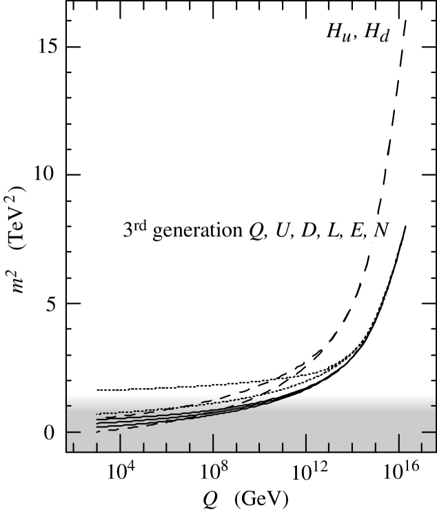
FIG. 1.: The renormalization group evolution of the Higgs (dashed) and third generation squark (solid) and slepton (dotted) squared masses in the MSSM with a right-handed neutrino for the boundary conditions of Eq. (15) with $h_{G}=2$ and $m_{N}=10^{13}\text{ GeV}$. First and second generation scalar masses (not shown) are approximately renormalization group invariant. At the weak scale, $m_{L}=1270\text{ GeV}$, $m_{E}=830\text{ GeV}$, $m_{H_{u}}=710\text{ GeV}$, $m_{D}=690\text{ GeV}$, $m_{Q}=570\text{ GeV}$, $m_{U}=420\text{ GeV}$, and $m_{H_{d}}=50\text{ GeV}$. Note, however, that neglected effects of order $m_{\rm light}^{2}$ modify solutions in the shaded region. The suppression factor for this case is $S=20$ (see text).

In our analysis, we have neglected effects of order $m_{\rm light}$, which clearly have little impact on the overall suppression of the scalar mass scale. They do, however, modify the RGEs at the weak scale when the scalar masses are of order $m_{\rm light}$. By omitting such effects, we forfeit the possibility of investigating a number of topics, including the details of electroweak symmetry breaking, as well as quantitative determinations of finite corrections to fermion masses and the residual fine-tuning required to keep the $Z$ mass light. Here, we note only that our scenario shares the problem of proper electroweak symmetry breaking generic to all supersymmetric scenarios with large $\tan\beta$ [16]. Several possible solutions have been discussed in the literature. For example, if the GUT group is broken not in one step, but in a chain beginning with $\text{SO(10)}\to\text{SU(5)}\times\text{U(1)}$, the resulting U(1) $D$-terms may help induce proper electroweak symmetry breaking [17]. These terms are parametrically of order $m_{\rm heavy}^{2}$, but are suppressed by the large $\text{U(1)}_{X}$ charge of the singlet. More generally, another source for ${\cal{O}}(m_{\rm light}^{2})$ (but not ${\cal{O}}(m_{\rm heavy}^{2})$) perturbations could be assumed.

The large radiatively-generated hierarchy evident in Fig. 1 exists for a wide range of parameters $m_{N}$ and $h_{G}$. To quantify the hierarchy, we characterize the scale of a given scalar spectrum at renormalization scale $Q$ by the quantity

$$\bar{m}^{2}(Q)\equiv{\rm Av}\left[\left|m^{2}(Q)\right|\right]\ ,$$ (19)

where the average is taken over all scalar fields in the theory, properly weighted by color and SU(2) factors. (This definition of $\bar{m}^{2}(Q)$ is invariant under possible shifts from $D$-terms.) We then define the suppression, or crunching, factor

$$S\equiv\frac{\bar{m}^{2}(M_{0})}{\bar{m}^{2}(m_{W})}\ ,$$ (20)

where the weak scale $m_{W}$ is taken to be 1 TeV. In Fig. 2 we plot $S$ in the $(m_{N},h_{G})$ plane. For a broad range of $h_{t}$ near its quasi-fixed point, we see that $S\sim 20$ is possible. For smaller values of $h_{t}$, the scalar masses do not approach their fixed point as quickly, and for larger values, two-loop effects become important. Indeed, the two-loop terms give positive contributions to $\dot{Y}$, and therefore increase the Yukawa suppression of scalar masses. However, they also give positive contributions directly to these masses. (See Eq. (17).) The latter effects dominate, so the two-loop terms degrade the hierarchy. For $h_{t}$ larger than shown in Fig. 2, the two-loop effects become so large that perturbation theory cannot be trusted.

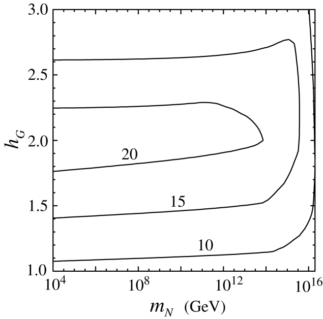
FIG. 2.: The suppression factor $S$ defined in the text for the MSSM with a right-handed neutrino $N$ with initial boundary conditions given by Eq. (15). The parameter $m_{N}$ is the scale at which the right-handed neutrino decouples, and $h_{G}$ is the value of the universal Yukawa coupling at the GUT scale $M_{G}\simeq 2\times 10^{16}$.

The definition of $S$ is, of course, somewhat arbitrary, but its size gives an indication of the reductions in the scalar masses that are possible from radiative effects. In particular, $S$ provides a rough measure of the reduction of the scalar contribution to fine-tuning and $\sqrt{S}$ is a measure of $m_{\rm heavy}/m_{\rm light}$. From Fig. 2 we see that, if values of $m_{\rm light}$ of order 1 TeV are considered natural, values of $m_{\rm heavy}$ up to $\sim 4\text{ TeV}$ are acceptable. This is then the scale of the matter fields of the first and second generation, which, given their small Yukawa couplings, do not renormalize significantly.

A scale of 4 TeV does not completely solve the most stringent flavor and $CP$ problems related to the $K$ system, but it does reduce them significantly with respect to the typical case with squark masses of 1 TeV. In addition, several of the other experimental difficulties mentioned in Sec. I are also resolved. Detecting scalars with such heavy masses will pose a serious challenge to future colliders.

Finally, we note that the values of $S$ are largely independent of $m_{N}$. For $m_{N}\lesssim 10^{13}\text{ GeV}$, the hierarchy is already created by the time the neutrino decouples, and so is insensitive to the decoupling scale. However, even for $m_{N}$ approaching $M_{G}$, a large hierarchy is possible. This may be understood as follows. When $N$ decouples, the new evolution matrix $\mbox{\boldmath$N$}^{\prime}$ is the upper $7\times 7$ block of $N$ with $Y_{n}=0$. The matrix $\mbox{\boldmath$N$}^{\prime}$ has 3 positive and 4 zero eigenvalues. In terms of $\cos 3\theta=17/64$, the 2 largest eigenvalues are $\frac{4}{3}(\cos\theta\pm\sqrt{3}\sin\theta+16)\approx 7.5,5.6$; their corresponding eigenvectors $\mbox{\boldmath$e$}^{\prime}_{1}$ and $\mbox{\boldmath$e$}^{\prime}_{2}$ are also quickly damped. If we decompose the 7-dimensional truncation of $\mbox{\boldmath$e$}_{1}$ into these new eigenvectors, $\mbox{\boldmath$e$}_{1}^{\rm tr}=(2,1,1,1,2,1,1)\equiv\sum_{i=1}^{7}c^{\prime}_{i}\mbox{\boldmath$e$}^{\prime}_{i}$, we find that the decomposition is dominated by $\mbox{\boldmath$e$}^{\prime}_{1}$ and $\mbox{\boldmath$e$}^{\prime}_{2}$ components: for the remaining components, $|\sum_{i=3}^{7}c^{\prime}_{i}\mbox{\boldmath$e$}^{\prime}_{i}|/|\mbox{\boldmath$e$}_{1}^{\rm tr}|=0.20$. Thus, the decoupling of $N$ perturbs the fixed point structure only slightly — when $N$ decouples, the scalar mass spectrum projects mainly on to the new eigenvectors with largest eigenvalues, and the rapid exponential damping continues. Note that the special case $m_{N}=M_{G}$ is equivalent to the case of an SU(5) GUT with universal Yukawa couplings and minimal SU(5) particle content. The exact eigenvectors for the SU(5) fixed point system are complicated. However, the above analysis shows that $\mbox{\boldmath$e$}_{1}^{\rm tr}$ is nearly a linear combination of eigenvectors with large eigenvalues, so large hierarchies can be generated from simple boundary conditions in the SU(5) case as well.

IV GUTs above the Unification Scale

An inverse hierarchy may also be generated in supergravity theories through renormalization group evolution above the unification scale. In this section we consider models in which scalar masses are generated at the supergravity scale, which we take to be the reduced Planck scale $M_{\ast}=2.4\times 10^{18}\text{ GeV}$, and then evolved to the GUT scale $M_{G}\simeq 2\times 10^{16}\text{ GeV}$. Even though the evolution interval is only two decades, we again find that substantial hierarchies may be created for simple initial scalar spectra. We will consider two generic cases for illustration.

A SO(10)

We begin by considering SO(10) models, that is, the class of models with superpotential

$$W=h_{t}\psi\psi{\cal H}_{2}+\ldots\ ,$$ (21)

where the matter fields are contained in $\psi$ ($16$) and both up-type and down-type Higgs fields are contained in a single multiplet: ${\cal H}_{2}$ ($10$) $\supseteq({\cal H}_{u},{\cal H}_{d})$, where ${\cal H}_{u}$, ${\cal H}_{d}$ are $5$ and $\bar{5}$ representations of the SU(5) subgroup, respectively. We allow arbitrary additional field content, subject only to the constraint that additional superpotential couplings are small relative to $h_{t}$. Note that two Higgs models, with superpotential $W=h_{t}\psi\psi{\cal H}_{2}+h_{b}\psi\psi{\cal H}_{1}+\ldots$ are, for the purposes of our analysis, equivalent to a one Higgs model in the limit $h_{t}=h_{b}$ (see Appendix). To the extent that the couplings are unified in this more general class of models, this analysis also applies.

The RGEs for this class of models are given in the Appendix. Note that additional interactions and an extended Higgs sector are required to break SO(10) and generate flavor structure. In general, this leads to a set of RGEs that are highly model-dependent. Fortunately, though, in the limit we consider, the RGEs simplify considerably. First, we assume that all additional Yukawa couplings are small, so their impact on the RGEs may be neglected. Second, the presence of additional fields with standard model quantum numbers modifies all RGE terms with two or more powers of $\tilde{\alpha}$. Fortunately, as argued in Sec. III, the two-loop terms of this form are highly suppressed. (We have checked that they are insignificant for reasonable field content.) Third, extra fields with standard model quantum numbers also change the one-loop $\beta$-function coefficient $b_{10}$. To good approximation, this is the only important effect, so the RGEs of these models may be studied simply by taking $b_{10}$ as an arbitrary free parameter. We will consider the range $-3\leq b_{10}\leq 20$, for which $1/26\lesssim\alpha(M_{\ast})\lesssim 1/8$.

We now proceed as in Sec. III. The one-loop scalar mass evolution is given by $\dot{\mbox{\boldmath$m$}}^{2}=-Y_{t}{\mbox{\boldmath$N$}}\mbox{\boldmath$m$}^{2}$, where

$${\mbox{\boldmath$N$}}=\left[\begin{array}[]{cc}4&8\\ 5&10\end{array}\right]\ ,$$ (22)

and ${\mbox{\boldmath$m$}^{2}}=(m_{{\cal H}_{2}}^{2},m_{\psi}^{2})^{T}$. The matrix $N$ has eigenvector $\mbox{\boldmath$e$}_{1}=(4,5)$ with eigenvalue 14, and another eigenvector with eigenvalue zero.

We therefore consider what hierarchies are possible, starting with initial boundary conditions

$$m_{{\cal H}_{2}}^{2}=\frac{4}{5}m_{\psi}^{2}\ .$$ (23)

The suppression factor $S$ is plotted in Fig. 3. Several features are worthy of note. First, $S$ is rather insensitive to $b_{10}$, but is slightly improved for large particle content. In addition, even though the scalar masses are never pushed negative, $S$ is degraded for very large $h_{\ast}=h_{t}(M_{\ast})$. As above, this is caused by two-loop effects. Nevertheless, even for initial Yukawa couplings $h_{\ast}\sim 2$, we see that $\sqrt{S}\sim 2$ is possible. Scalars at 2 TeV again ameliorate a number of problems, and also stretch the discovery limits of planned future colliders.

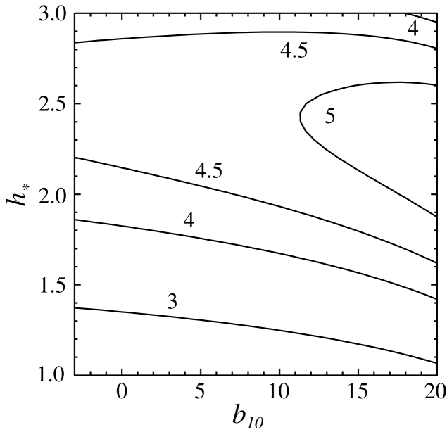
FIG. 3.: The suppression factor $S$ for SO(10) models evolving from $M_{\ast}=2.4\times 10^{18}\text{ GeV}$ to $M_{G}\simeq 2\times 10^{16}\text{ GeV}$ with boundary conditions given by Eq. (23). The parameter $b_{10}$ is the one-loop $\beta$-function coefficient parametrizing this class of models, and $h_{\ast}$ is the value of the universal Yukawa coupling at the scale $M_{\ast}$.

B SU(5)

Finally, we consider the minimal SU(5) model and extensions. The minimal SU(5) model has superpotential

$$W=\frac{1}{4}h_{t}TT{\cal H}_{u}+\sqrt{2}h_{b}TF{\cal H}_{d}+\ldots\ ,$$ (24)

where the quark and lepton fields are $T$ ($10$) and $F$ ($\bar{5}$) and the Higgs fields are ${\cal H}_{u}$ ($5$) and ${\cal H}_{d}$ ($\bar{5}$).

We assume that $h_{t}$ and $h_{b}$ are equal and large, and that all other couplings are small relative to these. Since we take $h_{t}$ and $h_{b}$ to be near their quasi-fixed points, the latter restriction is not too severe. Note that we must take $h_{t}$ and $h_{b}$ to be large in order to suppress $m_{H_{u}}$ and $m_{H_{d}}$. This was an automatic and attractive feature of the minimal SO(10) models.

The RGEs are given in the Appendix. In the minimal model, the $\beta$-function coefficient is $b_{5}=-3$; it is larger in extensions of the minimal model, and so, as before, we take it to be a free parameter.

The evolution matrix is

$${\mbox{\boldmath$N$}}=\left[\begin{array}[]{cccc}3&6&0&0\\ 3&8&2&2\\ 0&4&4&4\\ 0&4&4&4\end{array}\right]$$ (25)

in the basis ${\mbox{\boldmath$m$}^{2}}=(m_{{\cal H}_{u}}^{2},m_{T}^{2},m_{F}^{2},m_{{\cal H}_{d}}^{2})^{T}$, where $Y=Y_{t}=Y_{b}$. The leading eigenvector is $\mbox{\boldmath$e$}_{1}=(3,5,4,4)$, with eigenvalue 13. Suppression factors, with initial conditions

$$\frac{3}{4}m_{{\cal H}_{u}}^{2}=\frac{5}{4}m_{T}^{2}=m_{F}^{2}=m_{{\cal H}_{d}}^{2}\ ,$$ (26)

are plotted in Fig. 4. We find results similar to the SO(10) case. First and second generation scalar masses as large as 2 TeV are allowed. As before, they significantly reduce the stringency of the experimental constraints on scalar degeneracy and $CP$-violating phases.

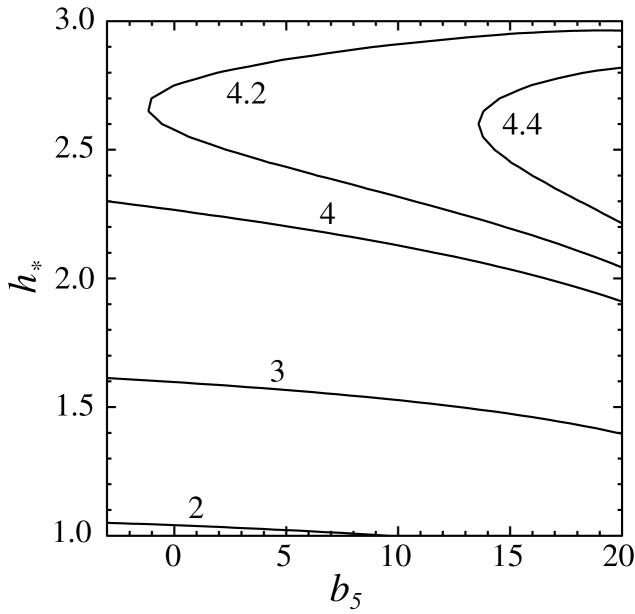
FIG. 4.: The suppression factor $S$, as in Fig. 3, but for SU(5) theories with the boundary conditions of Eq. (26).

V Conclusions

In this study we have examined the possibility that soft supersymmetry breaking scalar masses are of order $m_{\rm heavy}$ at some high scale. The third generation scalar masses are driven to $m_{\rm light}\lesssim\text{ TeV}$ in the infrared by their large Yukawa couplings, while first and second generation scalar masses remain at $m_{\rm heavy}$. This inverse hierarchy mechanism offers an appealing and natural way to satisfy the strong experimental constraints on first and second generation scalars in supersymmetric theories.

The third generation scalar masses are determined by infrared fixed points, so their precise values are insensitive to the initial conditions at, say, $M_{G}$ (or to the exact value of $M_{G}$, for that matter). We have shown that with suitable assumptions and approximations, the scalar fixed points may be extracted from the RGEs analytically. We justified the validity of these approximations by more precise numerical calculations.

For evolution below the GUT scale, we find that hierarchies of $m_{\rm heavy}/m_{\rm light}\sim 4$ may be created. The necessary boundary conditions are those of Eq. (15), with the Higgs squared masses double those of the squarks and sleptons. The simplicity of this boundary condition is in some sense a measure of the plausibility of the scenario. It is remarkable that such a simple boundary condition, perhaps the simplest imaginable next to complete scalar universality, allows one to move the entire scalar mass scale up to 4 TeV without sacrificing naturalness. Note that for simplicity we have focussed on only the eigenvectors with largest eigenvalue. However, other eigenvectors with non-zero eigenvalue are also crunched, and so initial conditions in these directions may also be acceptable. It would be interesting to find theories that naturally generate such boundary conditions and to investigate the fixed point structure of other models.

The scale $m_{\rm heavy}\sim 4\text{ TeV}$ eliminates many dangerous supersymmetric effects; for example, supersymmetric contributions to EDMs, which in these scenarios scale like $m_{\rm light}^{2}/m_{\rm heavy}^{4}$, may be easily below the experimental bounds even for ${\cal O}(1)$ phases. However, these hierarchies are not sufficient to completely satisfy the most stringent experimental bounds by themselves. For example, for $m_{\rm heavy}\sim 4\text{ TeV}$, the $K-\bar{K}$ mass difference still requires $m_{12}^{2}/m_{\rm heavy}^{2}\lesssim 0.1$, where $m_{12}^{2}$ is the off-diagonal entry of the squark mass matrix mixing the first and second generations. Nevertheless, such constraints are significantly weaker than in typical scenarios.

For evolution above the GUT scale, the brief evolution interval makes it impossible to generate such large hierarchies. However, $m_{\rm heavy}/m_{\rm light}\sim 2$ is possible, and constraints on scalar degeneracy and $CP$-violating phases are still significantly weakened relative to the standard scenario in which all scalars are below 1 TeV. Note that this is opposite to the typical situation is unified models, where ${\cal O}(1)$ generational splitting from unification-era evolution [18] can lead to new contributions to flavor [19, 20] and $CP$ violation [21]. (A similar situation occurs in the presence of a right-handed neutrino with a large Yukawa coupling [22].)

Throughout this analysis, we have neglected off-diagonal scalar squared masses. For the squark masses, constraints on $m_{12}$ have already been noted above. The off-diagonal elements $m_{13}$ and $m_{23}$ are also constrained: the requirement that the squark mass matrix be tachyon-free implies $m_{13}^{2},m_{23}^{2}\lesssim m_{\rm light}m_{\rm heavy}$. The off-diagonal masses are not driven to $m_{\rm light}$ and are, in fact, essentially RGE-invariant; the origins of their slight suppressions must therefore lie elsewhere. Depending on the extent of these suppressions, some interesting signals, for example, in the $B$ system, may be observable in the near future [23].

Finally, we draw some implications for high energy colliders. In these scenarios, as in all scenarios with inverted scalar hierarchies, scalars with mass $m_{\rm heavy}$ are beyond the reach of proposed colliders, such as the LHC and NLC, and can only be detected through their non-decoupling from super-oblique corrections [24]. A goal of supersymmetric collider studies is to precisely measure superparticle properties, and thereby determine the supersymmetric parameters at the weak scale. It is then hoped that hints about physics at even smaller distances can be found by evolving these parameters to very high energies. The fixed point analysis shows that in certain directions of parameter space, corresponding to eigenvectors of the scalar mass evolution matrix with large eigenvalues, even large masses at the high scale are exponentially suppressed when they are evolved to the weak scale. Accurate determination of high scale boundary conditions in these directions therefore requires extremely precise measurements.

In this appendix, we present the renormalization group equations for SU(5) and SO(10) GUTs above and below the GUT scale. As explained in Sec. III, gaugino masses and $A$ terms are negligible in the scenarios we are considering. The relevant parameters are then the gauge couplings $g$, Yukawa couplings $h$, and scalar squared masses $m^{2}$. The RGEs are conveniently expressed in terms of the variables

$$t \equiv \ln\left(M_{0}^{2}/Q^{2}\right)$$ (27)

$$\tilde{\alpha} \equiv \frac{g^{2}}{16\pi^{2}}=\frac{\alpha}{4\pi}$$ (28)

$$Y \equiv \frac{h^{2}}{16\pi^{2}}$$ (29)

$$X \equiv m_{X}^{2}\ ,$$ (30)

where, as indicated in Eq. (30), for notational simplicity we denote a scalar field’s squared mass by the field itself.

Schematically, the two-loop RGEs then have the form

$$\dot{\tilde{\alpha}} = \underline{b\tilde{\alpha}^{2}}+\underline{\tilde{\alpha}^{2}Y}+\tilde{\alpha}^{3}$$ (31)

$$\dot{Y} = Y\left[\underline{-Y}+\underline{\tilde{\alpha}}+\underline{Y^{2}}-\tilde{\alpha}Y-\tilde{\alpha}^{2}\right]$$ (32)

$$\dot{X} = X\left[\underline{-Y}+\underline{Y^{2}}-\tilde{\alpha}Y-\tilde{\alpha}^{2}\right]\ ,$$ (33)

where $\dot{(\ )}\equiv\frac{d}{dt}$. The constant $b$ is the one-loop $\beta$-function coefficient; the signs of all other terms are determined as indicated. Most of the two-loop terms are insignificant, as described in Sec. III. Below, we present all one-loop terms and the dominant two-loop terms underlined above.

1 MSSM with Right-handed Neutrino

The superpotential for the MSSM with a right-handed neutrino supermultiplet $N$ is

$$W=h_{t}H_{u}QU+h_{b}H_{d}QD+h_{\tau}H_{d}LE+h_{n}H_{u}LN\ .$$ (34)

The RGEs for the three (GUT normalized) gauge couplings are

$$\dot{\tilde{\alpha}}_{3} = 3\tilde{\alpha}_{3}^{2}+\tilde{\alpha}_{3}^{2}(4Y_{t}+4Y_{b})$$ (35)

$$\dot{\tilde{\alpha}}_{2} = -\tilde{\alpha}_{2}^{2}+\tilde{\alpha}_{2}^{2}(6Y_{t}+6Y_{b}+2Y_{\tau}+2Y_{n})$$ (36)

$$\dot{\tilde{\alpha}}_{1} = -\frac{33}{5}\tilde{\alpha}_{1}^{2}+\tilde{\alpha}_{1}^{2}\left(\frac{26}{5}Y_{t}+\frac{14}{5}Y_{b}+\frac{18}{5}Y_{\tau}+\frac{6}{5}Y_{n}\right)\ .$$ (37)

The Yukawa coupling RGEs are

$$\dot{Y}_{t} = Y_{t}\ [-6Y_{t}-Y_{b}-Y_{n}+\frac{16}{3}\tilde{\alpha}_{3}+3\tilde{\alpha}_{2}+\frac{13}{15}\tilde{\alpha}_{1}$$ (39)

$$\quad+22Y_{t}^{2}+5Y_{t}Y_{b}+3Y_{t}Y_{n}+5Y_{b}^{2}+Y_{b}Y_{\tau}+Y_{\tau}Y_{n}+3Y_{n}^{2}]$$

$$\dot{Y}_{b} = Y_{b}\ [-Y_{t}-6Y_{b}-Y_{\tau}+\frac{16}{3}\tilde{\alpha}_{3}+3\tilde{\alpha}_{2}+\frac{7}{15}\tilde{\alpha}_{1}$$ (41)

$$\quad+5Y_{t}^{2}+5Y_{t}Y_{b}+Y_{t}Y_{n}+22Y_{b}^{2}+3Y_{b}Y_{\tau}+3Y_{\tau}^{2}+Y_{\tau}Y_{n}]$$

$$\dot{Y}_{\tau} = Y_{\tau}\ [-3Y_{b}-4Y_{\tau}-Y_{n}+3\tilde{\alpha}_{2}+\frac{9}{5}\tilde{\alpha}_{1}$$ (43)

$$\quad+3Y_{t}Y_{b}+3Y_{t}Y_{n}+9Y_{b}^{2}+9Y_{b}Y_{\tau}+10Y_{\tau}^{2}+3Y_{\tau}Y_{n}+3Y_{n}^{2}]$$

$$\dot{Y}_{n} = Y_{n}\ [-3Y_{t}-Y_{\tau}-4Y_{n}+3\tilde{\alpha}_{2}+\frac{3}{5}\tilde{\alpha}_{1}$$ (45)

$$\quad+9Y_{t}^{2}+3Y_{t}Y_{b}+9Y_{t}Y_{n}+3Y_{b}Y_{\tau}+3Y_{\tau}^{2}+3Y_{\tau}Y_{n}+10Y_{n}^{2}]\ .$$

Finally, assuming that the hypercharge trace ${\rm tr}[Y^{\prime}m^{2}]$ vanishes, the scalar squared masses evolve as

$$\dot{Q} = -Y_{t}s_{1}-Y_{b}s_{2}+10Y_{t}^{2}s_{1}+10Y_{b}^{2}s_{2}+Y_{t}Y_{n}(s_{1}+s_{4})+Y_{b}Y_{\tau}(s_{2}+s_{3})$$ (46)

$$\dot{U} = -2Y_{t}s_{1}+16Y_{t}^{2}s_{1}+2Y_{t}Y_{b}(s_{1}+s_{2})+2Y_{t}Y_{n}(s_{1}+s_{4})$$ (47)

$$\dot{D} = -2Y_{b}s_{2}+16Y_{b}^{2}s_{2}+2Y_{t}Y_{b}(s_{1}+s_{2})+2Y_{b}Y_{\tau}(s_{2}+s_{3})$$ (48)

$$\dot{L} = -Y_{\tau}s_{3}-Y_{n}s_{4}+6Y_{\tau}^{2}s_{3}+6Y_{n}^{2}s_{4}+3Y_{t}Y_{n}(s_{1}+s_{4})+3Y_{b}Y_{\tau}(s_{2}+s_{3})$$ (49)

$$\dot{E} = -2Y_{\tau}s_{3}+8Y_{\tau}^{2}s_{3}+2Y_{\tau}Y_{n}(s_{3}+s_{4})+6Y_{b}Y_{\tau}(s_{2}+s_{3})$$ (50)

$$\dot{N} = -2Y_{n}s_{4}+8Y_{n}^{2}s_{4}+2Y_{\tau}Y_{n}(s_{3}+s_{4})+6Y_{t}Y_{n}(s_{1}+s_{4})$$ (51)

$$\dot{H}_{u} = -3Y_{t}s_{1}-Y_{n}s_{4}+18Y_{t}^{2}s_{1}+3Y_{t}Y_{b}(s_{1}+s_{2})+6Y_{n}^{2}s_{4}+Y_{\tau}Y_{n}(s_{3}+s_{4})$$ (52)

$$\dot{H}_{d} = -3Y_{b}s_{2}-Y_{\tau}s_{3}+18Y_{b}^{2}s_{2}+3Y_{t}Y_{b}(s_{1}+s_{2})+6Y_{\tau}^{2}s_{3}+Y_{\tau}Y_{n}(s_{3}+s_{4})\ ,$$ (53)

where

$$s_{1} \equiv H_{u}+Q+U$$ (54)

$$s_{2} \equiv H_{d}+Q+D$$ (55)

$$s_{3} \equiv H_{d}+L+E$$ (56)

$$s_{4} \equiv H_{u}+L+N\ .$$ (57)

These RGEs are valid above the right-handed neutrino mass scale $m_{N}$. The RGEs for the MSSM with minimal field content may be obtained, of course, by setting $Y_{n}=0$.

2 SO(10) above the GUT scale

In the text, we consider a class of minimal SO(10) models with only one large Yukawa coupling. Here, for completeness, we present RGEs for the more general class of models specified by the superpotential

$$W=h_{t}\psi\psi{\cal H}_{2}+h_{b}\psi\psi{\cal H}_{1}+\ldots\ ,$$ (58)

where the quark and lepton fields are contained in $\psi$ ($16$), and ${\cal H}_{2}$ ($10$) and ${\cal H}_{1}$ ($10$) are Higgs fields. In addition to the usual scalar mass terms, we also include the off-diagonal mass $m_{{\cal H}_{12}}^{2}({\cal H}_{1}^{\dagger}{\cal H}_{2}+{\cal H}_{2}^{\dagger}{\cal H}_{1})$, which is allowed by all symmetries and is generated even if it is initially set to zero. The RGEs presented here correct certain one-loop terms given in Ref. [19], where the effects of this term were omitted.

We consider models with arbitrary additional field content, but with interactions such that the dominant Yukawa couplings are $h_{t}$ and $h_{b}$. The RGEs are then

$$\dot{\tilde{\alpha}}=-b_{10}\tilde{\alpha}^{2}+\tilde{\alpha}^{2}(28Y_{t}+28Y_{b})\ ,$$ (59)

$$\dot{Y}_{t} = Y_{t}\ [-14Y_{t}-14Y_{b}+\frac{63}{2}\tilde{\alpha}+130Y_{t}^{2}+260Y_{t}Y_{b}+130Y_{b}^{2}]$$ (60)

$$\dot{Y}_{b} = Y_{b}\ [-14Y_{t}-14Y_{b}+\frac{63}{2}\tilde{\alpha}+130Y_{t}^{2}+260Y_{t}Y_{b}+130Y_{b}^{2}]\ ,$$ (61)

and

$$\dot{\psi} = -5Y_{t}u_{1}-5Y_{b}u_{2}-10Y_{tb}{\cal H}_{12}$$ (63)

$$+90Y_{t}^{2}u_{1}+90Y_{t}Y_{b}(u_{1}+u_{2})+90Y_{b}^{2}u_{2}+180(Y_{t}+Y_{b})Y_{tb}{\cal H}_{12}$$

$$\dot{{\cal H}}_{2} = -4Y_{t}u_{1}-4Y_{tb}{\cal H}_{12}$$ (65)

$$+80Y_{t}^{2}u_{1}+40Y_{t}Y_{b}(u_{1}+u_{2})+120Y_{t}Y_{tb}{\cal H}_{12}+40Y_{b}Y_{tb}{\cal H}_{12}$$

$$\dot{{\cal H}}_{1} = -4Y_{b}u_{2}-4Y_{tb}{\cal H}_{12}$$ (67)

$$+80Y_{b}^{2}u_{2}+40Y_{t}Y_{b}(u_{1}+u_{2})+120Y_{b}Y_{tb}{\cal H}_{12}+40Y_{t}Y_{tb}{\cal H}_{12}$$

$$\dot{{\cal H}}_{12} = -2Y_{tb}(u_{1}+u_{2})-2(Y_{t}+Y_{b}){\cal H}_{12}$$ (69)

$$+20Y_{t}Y_{tb}(3u_{1}+u_{2})+20Y_{b}Y_{tb}(3u_{2}+u_{1})+(20Y_{t}^{2}+120Y_{t}Y_{b}+20Y_{b}^{2}){\cal H}_{12}\ ,$$

where

$$u_{1} \equiv 2\psi+{\cal H}_{2}$$ (70)

$$u_{2} \equiv 2\psi+{\cal H}_{1}$$ (71)

$${\cal H}_{12} \equiv m_{{\cal H}_{12}}^{2}$$ (72)

$$Y_{tb}^{2} \equiv Y_{t}Y_{b}\ ,$$ (73)

and

$$b_{10}=-16+S(R)\ .$$ (74)

Common representations of SO(10) and their Dynkin indices are $10$ (1), $16$ (2), $45$ (8), $54$ (12), $120$ (28), and $126$ (35).

In minimal SO(10) models, both up-type and down-type Higgs multiplets are contained in one SO(10) multiplet: ${\cal H}_{2}$ ($10$) $\supseteq({\cal H}_{u},{\cal H}_{d})$, where ${\cal H}_{u}$ and ${\cal H}_{d}$ are $5$ and $\bar{5}$ representations of the SU(5) subgroup, respectively. The RGEs for these models are obtained by setting $h_{b}={\cal H}_{1}={\cal H}_{12}=0$ in the equations above. The RGEs above, however, are also applicable to models in which the Higgs fields are contained in two separate SO(10) representations, with ${\cal H}_{2}$ ($10$) $\supseteq({\cal H}_{u},\bar{{\cal H}_{u}})$ and ${\cal H}_{1}$ ($10$) $\supseteq(\bar{{\cal H}}_{d},{\cal H}_{d})$.

A useful consistency check follows from noting that, for $h_{t}=h_{b}=h/\sqrt{2}$ and ${\cal H}_{1}={\cal H}_{2}={\cal H}_{12}={\cal H}/2$, the two Higgs model reduces to a minimal model with Higgs field $({\cal H}_{2}+{\cal H}_{1})/\sqrt{2}$, and indeed, the resulting RGEs are identical to those for minimal models.

3 SU(5) above the GUT scale

We consider also the minimal SU(5) model and possible extensions. The minimal SU(5) model has superpotential

$$W=\frac{1}{4}h_{t}TT{\cal H}_{u}+\sqrt{2}h_{b}TF{\cal H}_{d}+\mu_{H}{\cal H}_{u}{\cal H}_{d}+\lambda{\cal H}_{u}\Sigma{\cal H}_{d}+\mu_{\Sigma}\text{ tr}\Sigma^{2}+\frac{1}{6}\lambda^{\prime}\text{ tr}\Sigma^{3}\ ,$$ (75)

where the quark and lepton fields are $T$ ($10$) and $F$ ($\bar{5}$) and the Higgs fields are ${\cal H}_{u}$ ($5$), ${\cal H}_{d}$ ($\bar{5}$), and $\Sigma$ ($24$).

The Yukawa couplings $h_{t}$ and $h_{b}$ are large and near their fixed point. We assume that all other couplings, such as $\lambda$, $\lambda^{\prime}$, $\mu_{H}$, and $\mu_{\Sigma}$, are small relative to these. The RGEs are then

$$\dot{\tilde{\alpha}}=-b_{5}\tilde{\alpha}^{2}+\tilde{\alpha}^{2}(12Y_{t}+14Y_{b})\ ,$$ (76)

$$\dot{Y}_{t} = Y_{t}\ [-9Y_{t}-4Y_{b}+\frac{96}{5}\tilde{\alpha}+54Y_{t}^{2}+24Y_{t}Y_{b}+32Y_{b}^{2}]$$ (77)

$$\dot{Y}_{b} = Y_{b}\ [-3Y_{t}-10Y_{b}+\frac{84}{5}\tilde{\alpha}+18Y_{t}^{2}+30Y_{t}Y_{b}+64Y_{b}^{2}]\ ,$$ (78)

and

$$\dot{T} = -3Y_{t}t_{1}-2Y_{b}t_{2}+36Y_{t}^{2}t_{1}+6Y_{t}Y_{b}(t_{1}+t_{2})+32Y_{b}^{2}t_{2}$$ (79)

$$\dot{F} = -4Y_{b}t_{2}+12Y_{t}Y_{b}(t_{1}+t_{2})+48Y_{b}^{2}t_{2}$$ (80)

$$\dot{{\cal H}}_{u} = -3Y_{t}t_{1}+36Y_{t}^{2}t_{1}+12Y_{t}Y_{b}(t_{1}+t_{2})$$ (81)

$$\dot{{\cal H}}_{d} = -4Y_{b}t_{2}+12Y_{t}Y_{b}(t_{1}+t_{2})+48Y_{b}^{2}t_{2}\ ,$$ (82)

where

$$t_{1} \equiv 2T+{\cal H}_{u}$$ (83)

$$t_{2} \equiv T+F+{\cal H}_{d}\ .$$ (84)

In the minimal model, $b_{5}=-3$ in Eq. (76). For extensions of the minimal model, the above equations apply (again, assuming no large Yukawas), with the modification

$$b_{5}=-3+S(R)\ ,$$ (85)

where $S(R)$ is the sum of the Dynkin indices of the additional fields. For convenience, a few typical SU(5) representations and their Dynkin indices are listed here: $5$ ($\frac{1}{2}$), $10$ ($\frac{3}{2}$), $15$ ($\frac{7}{2}$), $24$ (5), $45$ (12), $50$ ($\frac{35}{2}$), and $75$ (25).

REFERENCES

- [1] Recent quantitative discussions of constraints from the system are contained in J. A. Bagger, K. T. Matchev, and R. J. Zhang, Phys. Lett. B412, 77 (1997); C. R. Allton et al., hep-lat/9806016; M. Ciuchini et al., JHEP 9810, 008 (1998); R. Contino and I. Scimemi, hep-ph/9809437.
- [2] For example, see W. Fischler, S. Paban, and S. Thomas, Phys. Lett. B289, 373 (1992); T. Ibrahim and P. Nath, Phys. Rev. D57, 478 (1998); ibid., erratum, Phys. Rev. D58, 019901 (1998).
- [3] T. Moroi, Phys. Lett. B447, 75 (1999).
- [4] For example, see R. Arnowitt and P. Nath, Phys. Rev. Lett. 69, 725 (1992); ibid. hep-ph/9808465; J. Hisano, H. Murayama, and T. Yanagida, Nucl. Phys. B402, 46 (1993); T. Goto and T. Nihei, hep-ph/9808255; K. S. Babu and M. J. Strassler, hep-ph/9808447; K. S. Babu, J. C. Pati, and F. Wilczek, hep-ph/9812538.
- [5] G. D. Coughlan, W. Fischler, E. W. Kolb, S. Raby, and G. G. Ross, Phys. Lett. B131, 59 (1983).
- [6] J. Ellis, D. V. Nanopoulos, and M. Quiros, Phys. Lett. B174, 176 (1986); T. Moroi, M. Yamaguchi, and T. Yanagida, Phys. Lett. B342, 105 (1995); M. Kawasaki, T. Moroi, and T. Yanagida, Phys. Lett. B370, 52 (1996); and references therein.
- [7] For recent proposals, see, for example, L. Randall and R. Sundrum, hep-th/9810155; G. Giudice, M. Luty, H. Murayama, and R. Rattazzi, JHEP 9812, 027 (1998); A similar situation also arises in certain string frameworks, see V. S. Kaplunovsky and J. Louis, Phys. Lett. B306, 269 (1993).
- [8] M. Drees, Phys. Rev. D33, 1468 (1986); S. Dimopoulos and G. F. Giudice, Phys. Lett. B357, 573 (1995); A. Pomarol and D. Tommasini, Nucl. Phys. B466, 3 (1996); A. G. Cohen, D. B. Kaplan, and A. E. Nelson, Phys. Lett. B388, 588 (1996); K. Agashe and M. Graesser, Phys. Rev. D59, 015007 (1999); D. Wright, hep-ph/9801449.
- [9] G. Dvali and A. Pomarol, Phys. Rev. Lett. 77, 3728 (1996); ibid., Nucl. Phys. B522, 3 (1998).
- [10] R. N. Mohapatra and A. Riotto, Phys. Rev. D55, 1 (1997); R.-J. Zhang, Phys. Lett. B402, 101 (1997); A. E. Nelson and D. Wright, Phys. Rev. D56, 1598 (1997). J. Hisano, K. Kurosawa, and Y. Nomura, Phys. Lett. B445, 316 (1999).
- [11] H. P. Nilles and N. Polonsky, Phys. Lett. B412, 69 (1997); D. E. Kaplan, F. Lepeintre, A. Masiero, A. E. Nelson, and A. Riotto, hep-ph/9806430.
- [12] J. L. Feng, C. Kolda, and N. Polonsky, Nucl. Phys. B546, 3 (1999).
- [13] S. P. Martin and M. T. Vaughn, Phys. Rev. D50, 2282 (1994); Y. Yamada, Phys. Rev. D50, 3537 (1994); I. Jack, D. R. T. Jones, Phys. Lett. B333, 372 (1994).
- [14] J. L. Feng, N. Polonsky, and S. Thomas, Phys. Lett. B370, 95 (1996).
- [15] C. T. Hill, Phys. Rev. D24, 691 (1981).
- [16] For example, see M. Olechowski and S. Pokorski, Nucl. Phys. B404, 590 (1993); M. Carena, M. Olechowski, S. Pokorski, and C. E. M. Wagner, Nucl. Phys. B426, 269 (1994); M. Olechowski and S. Pokorski, Phys. Lett. B344, 201 (1995).
- [17] Y. Kawamura, H. Murayama, and M. Yamaguchi, Phys. Lett. B324, 52 (1994); R. Hempfling, Phys. Rev. D52, 4106 (1995); R. Rattazzi and U. Sarid, Phys. Rev. D53, 1553 (1996).
- [18] N. Polonsky and A. Pomarol, Phys. Rev. Lett. 73, 2292 (1994); ibid. Phys. Rev. D51, 6532 (1995).
- [19] R. Barbieri, L. Hall and A. Strumia, Nucl. Phys. B445, 219 (1995); P. Ciafaloni, A. Romanino, and A. Strumia, Nucl. Phys. B458, 3 (1996).
- [20] M. E. Gomez and H. Goldberg, Phys. Rev. D53, 5244 (1996).
- [21] For example, see S. Dimopoulos and L. J. Hall, Phys. Lett. B344, 185 (1995); R. Barbieri, A. Romanino, and A. Strumia, Phys. Lett. B369, 283 (1996).
- [22] F. Borzumati and A. Masiero, Phys. Rev. Lett. 57, 961 (1986); J. Hisano, T. Moroi, K. Tobe, and M. Yamaguchi, Phys. Rev. D53, 2442 (1996); J. Hisano and D. Nomura, Phys. Rev. D59, 116003 (1999).
- [23] A. G. Cohen, D. B. Kaplan, F. Lepeintre, and A. E. Nelson, Phys. Rev. Lett. 78, 2300 (1997).
- [24] K. Hikasa and Y. Nakamura, Zeit. für Physik C70, 139 (1996); ibid., 71, 356 (1996); H.-C. Cheng, J. L. Feng, and N. Polonsky, Phys. Rev. D56, 6875 (1997); ibid., 57, 152 (1998); M. M. Nojiri, K. Fujii, and T. Tsukamoto, Phys. Rev. D54, 6756 (1996); M. M. Nojiri, D. M. Pierce, and Y. Yamada, Phys. Rev. D57, 1539 (1998); S. Kiyoura, M. M. Nojiri, D. M. Pierce, and Y. Yamada, Phys. Rev. D58, 075002 (1998); E. Katz, L. Randall, and S.-F. Su, Nucl. Phys. B536, 3 (1998).