FISIST/6-99/CFIF

Yukawa Structure with Maximal Predictability


G.C. Branco, D. Emmanuel-Costa and R. González Felipe

Centro de Física das Interacções Fundamentais,
Departamento de Física, Instituto Superior Técnico
Av. Rovisco Pais, 1049-001 Lisboa, Portugal

A simple Ansatz for the quark mass matrices is considered, based on the assumption of a power structure for the matrix elements and the requirement of maximal predictability. A good fit to the present experimental data is obtained and the position of the vertex of the unitarity triangle, i.e. $(\bar{\rho},\bar{\eta})$, is predicted.

1 Introduction

Understanding the pattern of fermion masses and mixings is one of the fundamental questions in particle physics that still remain open. Several approaches have been suggested in the literature, leading to various Ansätze for fermion mass matrices [1, 2]. In particular, higher dimension couplings could explain the hierarchy of fermion masses and mixing angles [3, 4]. Indeed, nonrenormalizable couplings such as $h^{u}_{ij}u_{j}Q_{i}H_{2}(\theta/M_{2})^{n_{ij}}$, $h^{d}_{ij}d_{j}Q_{i}H_{1}(\theta/M_{1})^{n_{ij}}$ may provide effective Yukawa couplings with suppression factors of the form $\epsilon^{n_{ij}}_{u,d}=(\langle\theta\rangle/M_{2,1})^{n_{ij}}$, once a suitable field $\theta$ acquires a vacuum expectation value $\langle\theta\rangle$. Here $h^{u}_{ij},h^{d}_{ij}$ are coupling strengths, $u_{j},d_{j}$ denote the $SU(2)$ singlet quark fields, $Q_{i}$ are the quark doublets, $H_{1,2}$ are the Higgs fields for the up and down sectors and $M_{1,2}$ are mass scales which govern higher dimension operators. These effective Yukawa couplings can then lead to a hierarchical structure in the quark mass matrices depending on the underlying symmetries which constrain the powers $n_{ij}$. An example of such symmetries are gauge symmetries with an additional $U(1)$ symmetry [3, 4]. Another example is provided by symmetries of a compactified space coming from superstring theories [5, 6].

A figure of merit of any given Ansatz is its predictability power which, obviously, is maximal when a minimal number of free parameters is introduced. It is then natural to ask what is the maximal predictability one may achieve under some rather general assumptions. Using the minimal supersymmetric standard model (MSSM) as a guideline, let us assume that there are two Higgs doublets with vacuum expectation values $v_{u}$ and $v_{d}$. We then expect the up and down quark mass matrices to depend on two independent overall constants $a_{u}$ and $a_{d},$ which are directly related to $v_{u,d}$ but not to the flavor structure of Yukawa couplings. Moreover, if higher dimension couplings lead to suppression factors $\epsilon_{u,d}$ with some powers determined by quantum numbers of the underlying symmetries, then we expect in general that $\epsilon_{u}\neq\epsilon_{d}$ due to Higgs mixing [4].

From the above observations, it follows in general that maximal predictability in the quark sector is achieved if the quark mass matrices, apart from the overall constants $a_{u},a_{d}$, depend on two real parameters $\epsilon_{u,d}$ and a phase $\varphi$. The inclusion of a phase reflects, of course, the implicit assumption that the Kobayashi-Maskawa [8] mechanism is one of the sources of CP violation chosen by nature. Obviously, it does not exclude the existence of other sources of CP breaking.

In this letter we shall consider a simple string-inspired Ansatz for the quark mass matrices which, on one hand, has maximal predictability as defined above and, on the other, is in agreement with our present knowledge on the quark masses and the Cabibbo-Kobayashi-Maskawa (CKM) matrix at the electroweak scale. The predictive power of such an Ansatz can be appreciated by noting that since $a_{u},a_{d}$ drop out of quark mass ratios, the four independent quark mass ratios (two in each charge quark sector) and the four parameters of the CKM matrix are expressed in terms of only two real parameters and one phase.

2 Quark mass matrices at the unification scale

One of the difficulties in attempting to obtain the correct pattern for the Yukawa couplings stems from the fact that in the standard model (SM), as well as in the MSSM, the quark mass matrices contain a large redundancy. Indeed, if one starts from a given weak basis (WB) where the charged currents are diagonal and real, while the quark mass matrices $M_{u}$, $M_{d}$ are in general non-diagonal, then one is free to make a WB transformation under which $M_{u}\rightarrow M_{u}^{\prime}=W_{L}^{\dagger}\cdot M_{u}\cdot W_{uR},M_{d}\rightarrow M_{d}^{\prime}=W_{L}^{\dagger}\cdot M_{d}\cdot W_{dR},$ while the charged current remains diagonal and real. The two sets of mass matrices $(M_{u},M_{d}),(M_{u}^{\prime},M_{d}^{\prime})$ contain, of course, the same physics. If there is a fundamental symmetry principle responsible for the observed pattern of quark masses and mixings, only in an appropriate basis will this symmetry be “transparent”. In our search for a predictive and phenomenologically viable Yukawa structure, we will restrict ourselves to WB where $M_{u,d}$ are hermitian matrices. We will also choose the so-called heavy WB, where $M_{u,d}$ are both close to the chiral limit, i.e. $M_{u}=\text{diag}(0,0,m_{t})$ and $M_{d}=\text{diag}(0,0,m_{b})$. We will further assume a simple parallel power structure for the entries of the quark mass matrices $M_{u,d}$ at the grand unification (GUT) scale, so that deviations from the above chiral limit are measured by a small parameter $\epsilon$, which is of the order of the Cabibbo angle. Using simplicity and the requirement of maximal predictability as guiding principles, we are led to consider the following parallel structure for the up and down quark mass matrices at GUT scale:

$$M_{u,d}=a_{u,d}\,\left(\begin{array}[]{ccc}0&\epsilon_{u,d}^{3}&\epsilon_{u,d}^{4}\\ \epsilon_{u,d}^{3}&\epsilon_{u,d}^{2}&\epsilon_{u,d}^{2}\\ \epsilon_{u,d}^{4}&\epsilon_{u,d}^{2}&1\end{array}\right).$$ (1)

Let us note that such a structure can naturally arise e.g. within the framework of orbifold models [7] of superstring theory, where matter fields are assigned to $\theta^{k}$-twisted sectors and their corresponding fixed points (see e.g. Refs. [6] for details). We notice also that the coupling strengths $h^{u},h^{d}$, of the higher dimension operators are calculable in the framework of superstring theory and are typically of order $O(1)$. Although the (1,1)-matrix elements in $M_{u,d}$ do not completely vanish in this approach, they are usually strongly suppressed. Furthermore, they can be set to zero by means of an appropriate WB transformation [9].

In what follows we shall write the suppression factors $\epsilon_{u,d}$ in terms of a small expansion parameter $\epsilon$. We denote $\epsilon_{u}\equiv w^{2}\epsilon^{2}$ and $\epsilon_{d}\equiv\epsilon$, where $w=\sqrt{\epsilon_{u}}/\epsilon_{d}$ is a real parameter of order $O(1)$. Under these assumptions, the (1,3)-matrix element in $M_{u}$ will be suppressed compared to its neighboring elements. Therefore, we can write the quark mass matrices (1) in the following form:

$$M_{u} =a_{u}\,\left(\begin{array}[]{ccc}0&w^{6}\epsilon^{6}&0\\ w^{6}\epsilon^{6}&w^{4}\epsilon^{4}&w^{4}\epsilon^{4}\\ 0&w^{4}\epsilon^{4}&1\end{array}\right),$$ (5)

$$M_{d} =a_{d}\,\left(\begin{array}[]{ccc}0&\epsilon^{3}e^{-i\varphi_{1}}&\epsilon^{4}e^{-i\varphi_{2}}\\ \epsilon^{3}e^{i\varphi_{1}}&\epsilon^{2}&\epsilon^{2}e^{-i\varphi_{3}}\\ \epsilon^{4}e^{i\varphi_{2}}&\epsilon^{2}e^{i\varphi_{3}}&1\end{array}\right).$$ (9)

At this stage, it should be emphasized that the zeros in $M_{u}$ and $M_{d}$ have no physical meaning by themselves. Recently it has been shown [9] that in the Standard Model, starting from arbitrary matrices $M_{u}^{\prime}$, $M_{d}^{\prime}$, one can always make a WB transformation $M_{u}^{\prime}\rightarrow M_{u}=W_{L}^{\dagger}\cdot M_{u}^{\prime}\cdot W_{uR},M_{d}^{\prime}\rightarrow M_{d}=W_{L}^{\dagger}\cdot M_{d}^{\prime}\cdot W_{dR},$ which leads to $M_{u}$, $M_{d}$ with the zeros of Eqs. (5), (9). Furthermore, the texture zero structure of $M_{u}$ allows us to remove all phases in the up quark sector through a $U(1)$ WB transformation. We have kept three phases $\varphi_{i}\ (i=1,2,3)$ in $M_{d}$ in order not to loose generality. Of course, one could make a WB transformation which would render $M_{u}$ diagonal and real, while keeping $M_{d}$ hermitian. In that basis, only one meaningful phase would appear in $M_{d}$. Note also that the above $CP$-violating phases may dynamically arise in the context of superstring theories, e.g. from background antisymmetric tensors in orbifold models or imaginary vacuum expectation values of the $\theta$ field. The values of these phases may be further constrained by some extra symmetries, thus reducing the number of free parameters. Some examples are given in Section 3 where we present our numerical results.

The matrices $M_{u}$ and $M_{d}$ are diagonalized by the usual bi-unitary transformations $\ U_{u}^{\dagger}\cdot M_{u}\cdot U_{u}=D_{u},\ U_{d}^{\dagger}\cdot M_{d}\cdot U_{d}=D_{d},$ where $D_{u}=\text{diag}(-m_{u},m_{c},m_{t})$ and $D_{d}=\text{diag}(-m_{d},m_{s},m_{b})$. The CKM matrix $V$ is then given by $V=U_{u}^{\dagger}\cdot U_{d}$. From Eqs. (5) and (9) one derives the following approximate hierarchical relations for the up and down quark masses

$$m_{t}:m_{c}:m_{u} \approx 1:w^{4}\epsilon^{4}:w^{8}\epsilon^{8},$$

$$m_{b}:m_{s}:m_{d} \approx 1:\epsilon^{2}:\epsilon^{4}.$$ (10)

Furthermore, one obtains the two mass relations:

$$m_{u}m_{t}\approx m_{c}^{2}\quad,\quad m_{d}m_{b}\approx m_{s}^{2}.$$ (11)

Let us now consider the quark flavor mixings predicted by the Ansatz (5), (9). We can analytically determine the CKM matrix elements in powers of $\epsilon$. We obtain

$$|V_{ud}| \approx|V_{cs}|\approx 1-\frac{\epsilon^{2}}{2}\ ,$$

$$|V_{us}| \approx\left|V_{cd}\right|\approx\epsilon-w^{2}\epsilon^{2}\cos\varphi_{1}\ ,$$

$$\left|V_{ub}\right| \approx\epsilon^{4}\sqrt{1-2w^{2}\cos(\varphi_{2}-\varphi_{3})+w^{4}}\ ,$$ (12)

$$\left|V_{cb}\right| \approx\left|V_{ts}\right|\approx\epsilon^{2}-w^{4}\epsilon^{4}\cos\varphi_{3}+\frac{\epsilon^{4}}{2}\ ,$$

$$\left|V_{td}\right| \approx\epsilon^{3}-\epsilon^{4}\cos(\varphi_{1}-\varphi_{2}+\varphi_{3})\ ,$$

$$\left|V_{tb}\right| \approx 1-\frac{\epsilon^{4}}{2}\ .$$

Using the fact that one has $\epsilon\approx\sqrt{m_{d}/m_{s}}\$, $w^{2}\epsilon^{2}\approx\sqrt{m_{u}/m_{c}}\$, $|V_{us}|$ can also be written as:

$$|V_{us}|\approx\left|e^{-i\varphi_{1}}\sqrt{\frac{m_{d}}{m_{s}}}-\,\sqrt{\frac{m_{u}}{m_{c}}}\ \right|\ .$$ (13)

For the parameters of the unitarity triangle we obtain:

$$J =\text{Im}(V_{us}V_{ub}^{\ast}V_{cs}^{\ast}V_{cb})\approx\epsilon^{7}\ (w^{2}\sin\varphi_{1}-\sin(\varphi_{1}-\varphi_{2}+\varphi 3))\ ,$$

$$\bar{\rho} =-\text{Re}\left(\frac{V_{ud}V_{ub}^{\ast}}{V_{cd}V_{cb}^{\ast}}\right)\approx\epsilon\ (-w^{2}\cos\varphi_{1}+\cos(\varphi_{1}-\varphi_{2}+\varphi_{3}))\ ,$$ (14)

$$\bar{\eta} =-\text{Im}\left(\frac{V_{ud}V_{ub}^{\ast}}{V_{cd}V_{cb}^{\ast}}\right)\approx\epsilon\ (w^{2}\sin\varphi_{1}-\sin(\varphi_{1}-\varphi_{2}+\varphi_{3}))\ .$$

Finally, the angles of the unitarity triangle read as

$$\sin 2\alpha =\frac{2\bar{\eta}[\bar{\eta}^{2}+\bar{\rho}(\bar{\rho}-1)]}{[\bar{\eta}^{2}+(1-\bar{\rho})^{2}](\bar{\eta}^{2}+\bar{\rho}^{2})}$$

$$\approx\frac{\sin(2\varphi_{1}-2\varphi_{2}+2\varphi_{3})-2w^{2}\sin(2\varphi_{1}-\varphi_{2}+\varphi_{3})+w^{4}\sin(2\varphi_{1})}{1-2w^{2}\cos(\varphi_{2}-\varphi_{3})+w^{4}}\ ,$$

$$\sin 2\beta =\frac{2\bar{\eta}(1-\bar{\rho})}{\bar{\eta}^{2}+(1-\bar{\rho})^{2}}$$ (15)

$$\approx 2w^{2}\epsilon\sin\varphi_{1}-2\epsilon\sin(\varphi_{1}-\varphi_{2}+\varphi_{3})\ ,$$

$$\sin^{2}\gamma =\sin^{2}(\alpha+\beta).$$

Note that by definition $\alpha+\beta+\gamma=\pi$.

3 Quark masses and mixings at the electroweak scale

In order to compare the quark masses and mixings predicted by the Ansatz (5)-(9) with the present experimental data, it is necessary to run the quark masses and mixings from the unification scale ($M_{X}\sim 10^{16}$ GeV) down to the electroweak scale ($M_{Z}\sim 91$ GeV). For this purpose, we will use the renormalization group equations (RGE) for Yukawa couplings and the CKM matrix in the framework of the MSSM [14]. At this point, a few remarks are in order. The hierarchy of Yukawa couplings and quark mixing angles leads to the following:

1. The running effects of the ratios $m_{u}/m_{c}$ and $m_{d}/m_{s}$ are negligible small. This implies that the parameters $\epsilon_{u}\sim\sqrt{m_{u}/m_{c}}$ and $\epsilon_{d}\sim\sqrt{m_{d}/m_{s}}$ are mainly scale-independent.

2. The diagonal elements of the CKM matrix, i.e. $|V_{ud}|,|V_{cs}|,|V_{tb}|$, have negligible evolution with energy.

3. The evolution of $|V_{us}|$ and $|V_{cd}|$ involves second family Yukawa couplings and thus they are negligible.

4. The elements $|V_{ub}|$, $|V_{cb}|$, $|V_{td}|$ and $|V_{ts}|$ have identical running behaviours. In particular, this implies that the ratios $|V_{ub}/V_{cb}|$, $|V_{td}/V_{ts}|$, as well as the parameters $\bar{\rho},\bar{\eta}$ and the three inner angles of the unitarity triangle $\alpha,\beta,\gamma$, are approximately scale-independent to a good degree of accuracy.

Taking the above remarks into account, we are now in position to compare the predictions of our Ansatz with the present experimental data. We proceed as follows. We take as input values for the light quark masses the following values at 1 GeV [15]:

$$m_{u}=5.1\pm 0.9\text{ MeV}\ ,\quad m_{d}=9.3\pm 1.4\text{ MeV}\ ,\quad m_{s}=175\pm 25\text{ MeV}\ ,$$

while for the heavy quark masses we use the following ones [11]:

$$m_{c}(m_{c})=1.25\pm 0.15\text{ GeV}\ ,\quad m_{b}(m_{b})=4.25\pm 0.15\text{ GeV}\ ,$$

$$m_{t}=173.8\pm 5.2\text{ GeV}\ .$$

Then we find the running quark masses at $M_{Z}$ scale using the QCD RGE. Finally, using as input values the quark masses $m_{q}(M_{Z})$ and the present limits [11] on the CKM matrix parameters $|V_{ij}|$ we are able to compute the allowed range for the quark masses and mixings at GUT scale. The latter values are then compared with the ones predicted by the Ansatz (5)-(9).

To show that the present Ansatz is phenomenologically viable, next we present some numerical examples. For definiteness, we will take some simple choices for the phases, namely in case I we consider $\varphi_{k}=2k\pi/3$ and in case II, $\varphi_{2}-\varphi_{1}=\pi/2\ ,\ \varphi_{3}=0$, with $\varphi_{1}$ an arbitrary phase. These “geometrical” values for the phases could arise in principle from the presence of extra symmetries.

Case I:  $\varphi_{k}=2k\pi/3$

As a numerical example, let us take as input parameters $a_{u}=120$ GeV, $a_{d}=0.9$ GeV, $\epsilon=0.19$, $w=1.22$ and assume that $\varphi_{k}=2k\pi/3,\ k=1,2,3$. In this case, the diagonalization of the mass matrices (5) and (9) yields the following mass spectrum at the GUT scale $M_{X}\simeq 10^{16}$ GeV:

$$m_{u}=1\text{ MeV},\quad m_{c}=0.34\text{ GeV},\quad m_{t}=120\text{ GeV},$$

$$m_{d}=1.2\text{ MeV},\quad m_{s}=32.5\text{ MeV},\quad m_{b}=0.9\text{ GeV},$$ (16)

and the CKM matrix

$$|V|=\left(\begin{array}[]{ccc}0.9759&0.2180&0.0028\\ 0.2180&0.9754&0.0344\\ 0.0069&0.0338&0.9994\end{array}\right).$$ (17)

We notice that the values of the matrix elements $|V_{ub}|$, $|V_{cb}|$, $|V_{td}|$ and $|V_{ts}|$ at GUT scale are smaller than the corresponding ones at the electroweak scale by 10-15%. This is always the case in the MSSM.

Finally we can evaluate $J$, $\bar{\rho}$ and $\bar{\eta}$ as defined in Eqs. (14) to obtain $J=1.88\times 10^{-5},\quad\bar{\rho}=0.14,\quad\bar{\eta}=0.33,$ which are within the present experimental limits [12, 13]. The angles of the unitarity triangle are then predicted from Eqs. (15) and one obtains $\sin 2\alpha=-0.03,\quad\sin 2\beta=0.675,\quad\sin^{2}\gamma=0.86\,.$

Case II:  $\varphi_{2}-\varphi_{1}=\pi/2\ ,\ \varphi_{3}=0$

Let us take as input parameters $a_{u}=120$ GeV, $a_{d}=0.9$ GeV, $\epsilon=0.19$, $w=1.2$ and also $\varphi_{1}=2.2,\ \varphi_{2}=\varphi_{1}+\pi/2,\ \varphi_{3}=0$. In this case we obtain the following mass spectrum at the GUT scale:

$$m_{u}=0.88\text{ MeV},\quad m_{c}=0.32\text{ GeV},\quad m_{t}=120\text{ GeV},$$

$$m_{d}=1.17\text{ MeV},\quad m_{s}=32.4\text{ MeV},\quad m_{b}=0.9\text{ GeV},$$ (18)

while for the CKM matrix

$$|V|=\left(\begin{array}[]{ccc}0.9755&0.2201&0.0030\\ 0.2201&0.9749&0.0345\\ 0.0064&0.0341&0.9994\end{array}\right).$$ (19)

Moreover, $J=1.84\times 10^{-5},\quad\bar{\rho}=0.23,\quad\bar{\eta}=0.32,$ and the angles of the unitarity triangle are $\sin 2\alpha=-0.44,\quad\sin 2\beta=0.705,\quad\sin^{2}\gamma=0.66$, which are in good agreement with the present experimental limits.

The results presented in the above numerical examples are exact, no approximations have been made. The physical implications of the present Ansatz can be readily understood. It can easily be seen that, in leading order, the phases do not affect the quark mass spectrum which, apart from the overall constants $a_{u},a_{d}$, depends only on $\epsilon_{u,d}$. Once $\epsilon_{u,d}$ are determined from the observed quark mass spectrum, one can find $\varphi_{1}$ from Eq. (13), using the fact that $|V_{us}|$ is experimentally known with high precision. All the other CKM matrix elements are then predicted, in particular the values of $\bar{\rho}$ and $\bar{\eta}.$

In Fig. 1, we show the predictions for $\bar{\rho},\bar{\eta}$ implied by the Ansatz considered in this letter, corresponding to Eqs.(5),(9) and assuming $\varphi_{2}-\varphi_{1}=\pi/2\ ,\ \varphi_{3}=0$; $\varphi_{1}$ is an arbitrary phase (Case II). We have taken into account the allowed range for the quark mass spectrum and the CKM matrix elements [11], in particular the value of $|V_{us}|$. There are several constraints on $\bar{\rho}$, $\bar{\eta}$ arising from a variety of sources (see e.g. [12, 13] for details). We see from the figure that there exists a range of values for $\bar{\rho}$ and $\bar{\eta}$ (dark dotted area) which is consistent with the presently allowed region in the $\bar{\rho}-\bar{\eta}$ plane. Furthermore, it is clear that the Ansatz predicts that the values of $\bar{\rho}$, $\bar{\eta}$ should lie in a rather small region. This is a consequence of the constraints imposed on the $CP$-violating phases $\varphi_{k}$. Fig. 2 shows the same plot as Fig. 1 but for arbitrary $CP$-violating phases $\varphi_{1},\,\varphi_{2}$ and for a vanishing phase $\varphi_{3}$. We note that by relaxing the constraints on the phases the predicted area by the Ansatz (Eqs.(5),(9)) and the experimentally allowed area in the $(\bar{\rho},\bar{\eta})$-plane overlap in a wider region.

In conclusion, we have shown that it is possible to have a simple pattern for the Yukawa couplings, leading to a power structure for the elements of the quark mass matrices, which is in good agreement with the current experimental data on quark masses and mixings. Moreover, the pattern considered here has maximal predictability in the sense that the four independent quark mass ratios and the four physical parameters of the CKM matrix are given in terms of only two real parameters (case I) or two real parameters and one phase (Case II). The Ansatz predicts that the location of the vertex of the unitarity triangle should be confined to a specific region in the $\bar{\rho}-\bar{\eta}$ plane. These predictions will soon be tested in the forthcoming experiments at $B$-factories, through the measurement of $CP$ asymmetries in $B^{0}$-decays.

Acknowledgement

One of us (D.E.C.) would like to thank the Fundação de Ciência e Tecnologia (Segundo Quadro Comunitário de Apoio) for financial support under the contract No. Praxis XXI/BD/9487/96.

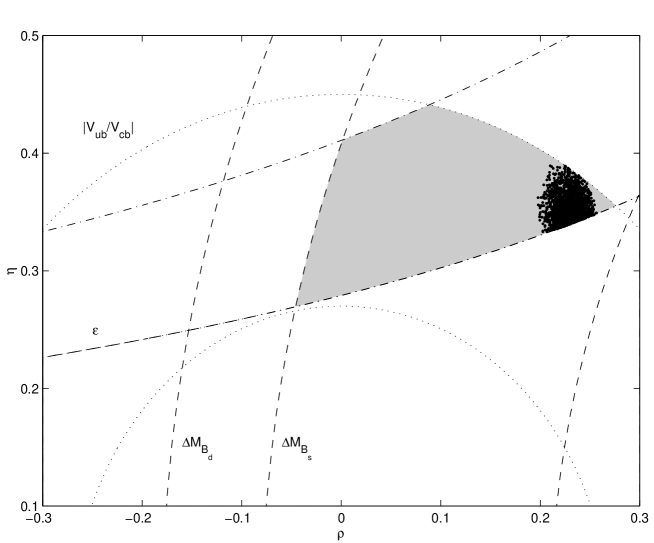
Figure 1: Allowed region (dark dotted area) in the $(\bar{\rho},\bar{\eta})$-plane for the Ansatz (Eqs.(5),(9)) considered in this letter. We have assumed $\varphi_{2}-\varphi_{1}=\pi/2,\ \varphi_{3}=0$; $\varphi_{1}$ is an arbitrary phase (Case II). The shaded-in area to the right of the $\Delta M_{B_{s}}$ curve corresponds to the experimentally allowed region in the SM, taking into account the experimental values of $\left|\varepsilon\right|,$ $\left|V_{ub}/V_{cb}\right|$, $\Delta M_{B_{d}}$ and the lower bound on $\Delta M_{B_{s}}$.

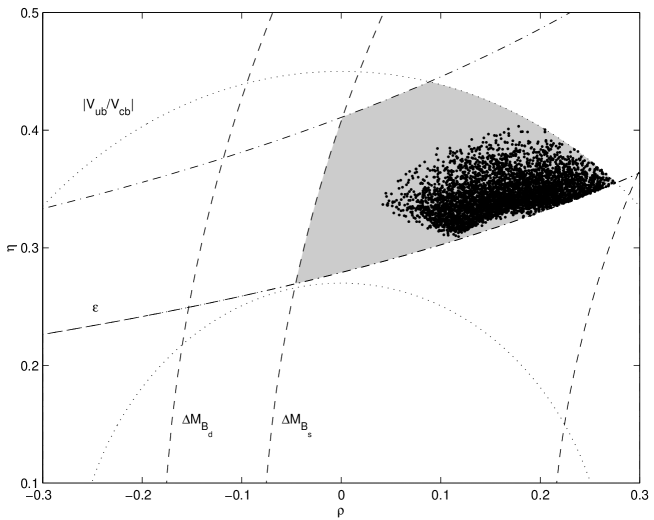
Figure 2: The same plot as in Fig. 1 but for arbitrary $CP$-violating phases $\varphi_{1},\,\varphi_{2}$. The phase $\varphi_{3}$ is assumed to be zero.

References

- [1] S. Weinberg, in Transactions of the New York Academy of Sciences 38 (1977) 185; F. Wilczek and A. Zee, Phys. Lett. 70B (1977) 418; H. Fritzsch, Phys. Lett. 70B (1977) 436. For a review and extended list of early references, see: R. Gatto, G. Morchio and G. Strochi, Nucl. Phys. B163 (1980) 221.
- [2] Recent references include: H. Fritzsch and J. Plankl, Phys. Lett. B 237 (1990) 446; S. Dimopoulos, L. Hall and S. Raby, Phys. Rev. Lett. 68 (1992) 1984; ibid, Phys. Rev. D 45 (1992) 4195; G.F. Giudice, Mod. Phys. Lett. A 7 (1992) 2429; P. Ramond, R. G. Roberts and G. G. Ross, Nucl. Phys. B406 (1993) 19; G.C. Branco and J.I. Silva-Marcos, Phys. Lett. B 331 (1994) 390; H. Fritzsch and Z.Z. Xing, Phys. Lett. B 353 (1995) 114; H. Harayama, N. Okamura, A.I. Sanda and Z.Z. Xing, Prog. Theor. Phys. 97 (1997) 781; G.C. Branco, D. Emmanuel-Costa and J.I. Silva-Marcos, Phys. Rev. D 56 (1997) 107; Y. Koide, Mod. Phys. Lett. A 12 (1997) 2655; R. Barbieri, L.J.Hall and A. Romanino, Nucl. Phys. B551 (1999) 93.
- [3] C.D. Froggatt and H.B. Nielsen, Nucl. Phys. B147 (1979) 277; S. Dimopoulos, Phys. Lett. B 129 (1983) 417; M. Leurer, Y. Nir and N. Seiberg, Nucl. Phys. B398 (1993) 319; ibid. B420 (1994) 468; Y. Nir and N. Seiberg, Phys. Lett. B 309 (1993) 337; P. Binétruy and P. Ramond, Phys. Lett. B 350 (1995) 49; E. Dudas, S. Pokorski and C.A. Savoy, Phys. Lett. B 356 (1995) 45.
- [4] L. Ibañez and G.G. Ross, Phys. Lett. B 332 (1994) 10.
- [5] J.L. Lopez and D.V. Nanopoulos, Nucl. Phys. B338(1990) 73; A.E. Faraggi and E. Halyo, Nucl. Phys. B416 (1994) 63; N. Haba, C. Hattori, M. Matsuda and T. Matsuoka, Prog. Theor. Phys. 96 (1996) 1249; K.S. Babu and R.N. Mohapatra, Phys. Rev. Lett. 74 (1995) 2418.
- [6] T. Kobayashi, Phys. Lett. B 354 (1995) 264; ibid. B 358 (1995) 253; T. Kobayashi and Z.Z. Xing, Mod. Phys. Lett. A 12 (1997) 561.
- [7] L. Dixon, J. Harvey, C. Vafa and E. Witten, Nucl. Phys. B261 (1985) 678; ibid. Nucl. Phys. B274 (1986) 285; L.E. Ibáñez, J. Mas, H.P. Nilles and F. Quevedo, Nucl. Phys. B301 (1988) 157.
- [8] M. Kobayashi and T. Maskawa, Prog. Theor. Phys. 49 (1973) 652.
- [9] G.C. Branco, D. Emmanuel-Costa and R. González Felipe, preprint FISIST/19-99/CFIF [hep-ph/9911418] (to appear in Phys. Lett. B).
- [10] The BaBar Physics Book: Physics at an Asymmetric B Factory, by BaBar Collaboration (P.F. Harrison, ed. et al.), SLAC-R-0504 (1998).
- [11] C. Caso et al., (Particle Data Group), Eur. Phys. J. C 3 (1998) 1.
- [12] A. Ali and D. London, Eur. Phys. J. C 9 (1999) 687; A. Ali and D. London, contribution to the Festschrift for L.B. Okun, to appear in a special issue of Physics Reports, eds. V.L. Telegdi and K. Winter [hep-ph/9907243].
- [13] F. Caravaglios, F. Parodi, P. Rodeau and A. Stocchi, preprint LAL 00-04 (February 2000) [hep-ph/0002171].
- [14] E. Ma and S. Pakvasa, Phys. Lett. B 86 (1979) 43; Phys. Rev. D 20 (1979) 2899; K. Sasaki, Z. Phys. C 32 (1986) 149; K.S. Babu, Z. Phys. C 35 (1987) 69; K.S. Babu and Q. Shafi, Phys. Rev. D 47 (1993) 5004.
- [15] H. Leutwyler, Phys. Lett. B 378 (1996) 313.
- [16] E. Derman and H.S. Tsao, Phys. Rev. D 20 (1979) 1207.