Application of Pauli–Villars Regularization and Discretized Light-Cone Quantization to a ($3+1$)-Dimensional Model

Abstract

We apply Pauli–Villars regularization and discrete light-cone quantization to the nonperturbative solution of a ($3+1$)-dimensional model field theory. The matrix eigenvalue problem is solved for the lowest-mass state with use of the complex symmetric Lanczos algorithm. This permits the calculation of each Fock-sector wave function, and from these we obtain values for various quantities, such as average multiplicities and average momenta of constituents, structure functions, and a form factor slope.

I Introduction

One of the most challenging problems in particle physics is the computation of the spectrum and physical properties of bound states in quantum field theory. The main tool presently used for such nonperturbative computations in quantum chromodynamics is lattice gauge theory[1], which has been highly successful for determining hadron spectra. However, the computation of dynamical properties, such as CP violation in weak transition matrix elements[2] or the shape of the distributions measured in deep inelastic scattering is difficult using standard lattice methods.

Light-cone Hamiltonian diagonalization methods[4] appear to provide a number of attractive advantages for solving nonperturbative problems in quantum field theory, including a Minkowski space description, boost invariance, no fermion-doubling, and a consistent Fock state expansion well matched to physical problems in QCD; however, thus far, full dynamical solutions based on light-cone Hamiltonian diagonalization have been primarily limited to one-space/one-time models. One promising approach is the transverse lattice which combines light-cone methods in the longitudinal light-cone direction with a spacetime lattice for the transverse dimensions.[3]

In recent work[5] we have shown that a model field theory in $3+1$ dimensions can be solved using discrete light-cone quantization (DLCQ)[6, 4], a light-cone Hamiltonian diagonalization method, together with Pauli–Villars regulation of the ultraviolet[7]. The particular model theory which we constructed has an exact analytic solution by which the DLCQ results could be checked, for both accuracy and rapidity of convergence. The model was regulated in the ultraviolet by a single Pauli–Villars boson, which was included in the DLCQ Fock basis in the same way as the “physical” particles of the theory. The two bare parameters of the model were then determined by fits of observables to chosen values.

Here we shall extend this combination of DLCQ and Pauli–Villars regularization to a more realistic model which mimics many features of a full quantum field theory. Unlike the analytic model which contained a static source, the light-cone energies of the particles in the new model have the correct longitudinal and transverse momentum dependence. Although an analytic solution of the new model is no longer available, the numerical convergence of the discretized light-cone solutions is found to be quite rapid, and the structure of the solution for the lowest-mass eigenstate is readily obtained. In particular, we can calculate the light-cone wavefunction of each Fock-sector component, and from these we can compute the values for various physical quantities, such as average multiplicities and average momenta of constituents, bosonic and fermionic structure functions, and a form factor slope.

A distinct advantage of our approach is that almost all counterterms are generated automatically by the Pauli–Villars particles and their imaginary couplings. This can be explicitly checked for consistency in perturbation theory. For nonperturbative calculations we conjecture that the same number of Pauli–Villars fields will be sufficient to regulate the theory. This does appear to be the case here and in the work reported previously[5]. An alternative procedure has been proposed and explored by Wilson, Perry and collaborators[8]; they use a similarity transformation to generate effective Hamiltonians perturbatively which can then be diagonalized in the valence Fock sector.

In our approach one can obtain the full set of Fock-sector wave functions for the lowest-mass eigenstate. This contrasts with other DLCQ calculations in $3+1$ dimensions[9, 10, 11] where the number of particles was severely limited from the outset and effects of higher Fock sectors can only be estimated. The DLCQ calculation by Wivoda and Hiller[12], though untruncated, did not construct counterterms in a way that can be systematically extended to other theories. In our case, a Tamm–Dancoff truncation[13] in particle number can be applied, and the impact of the truncation can be studied and understood.

Our notation is such that we define light-cone coordinates[14] by

$$x^{\pm}=x^{0}+x^{3}\,,\;\;\mathchoice{{\hbox{\boldmath$\displaystyle x$}}}{{\hbox{\boldmath$\textstyle x$}}}{{\hbox{\boldmath$\scriptstyle x$}}}{{\hbox{\boldmath$\scriptscriptstyle x$}}}_{\perp}=(x^{1},x^{2})\,.$$ (1)

The time coordinate is taken to be $x^{+}$. The dot product of two four-vectors is

$$p\cdot x=\frac{1}{2}(p^{+}x^{-}+p^{+}x_{-})-\mathchoice{{\hbox{\boldmath$\displaystyle p$}}}{{\hbox{\boldmath$\textstyle p$}}}{{\hbox{\boldmath$\scriptstyle p$}}}{{\hbox{\boldmath$\scriptscriptstyle p$}}}_{\perp}\cdot\mathchoice{{\hbox{\boldmath$\displaystyle x$}}}{{\hbox{\boldmath$\textstyle x$}}}{{\hbox{\boldmath$\scriptstyle x$}}}{{\hbox{\boldmath$\scriptscriptstyle x$}}}_{\perp}\,.$$ (2)

Thus the momentum component conjugate to $x^{-}$ is $p^{+}$, and the light-cone energy is $p^{-}$. We use underscores to identify light-cone three-vectors, such as

$$\underline{p}=(p^{+},\mathchoice{{\hbox{\boldmath$\displaystyle p$}}}{{\hbox{\boldmath$\textstyle p$}}}{{\hbox{\boldmath$\scriptstyle p$}}}{{\hbox{\boldmath$\scriptscriptstyle p$}}}_{\perp})\,.$$ (3)

For additional details, see Appendix A of Ref. [5] or a review paper [4].

The model which we study is defined in Sec. II. There we also list and define various quantities which we will compute from the eigensolution, including structure functions and distribution amplitudes, average multiplicities, and average momenta. The numerical methods, including the DLCQ procedure, and the results are discussed in Sec. III. Section IV contains some concluding remarks and plans for future work.

II A Model with a Dynamical Source

We shall consider a field-theoretic model where one particle, which we take to be a fermion of mass $M$, acts as a dynamical source and sink for bosons of mass $\mu$. The model is only slightly more complicated than the analytically soluble model considered in Ref. [5], the key difference being that here the fermion has a proper, momentum-dependent light-cone energy. Another difference is that the vertices do not include the momentum ratios which were introduced in[5] to control end-point behavior; the restoration of fermion dynamics makes such factors unnecessary. The theory is still regulated by a single Pauli–Villars boson with imaginary couplings and a mass $\mu_{1}$. The light-cone Hamiltonian (or mass-squared operator) $H_{\rm LC}=P^{+}P^{-}-P_{\perp}^{2}$ is, in the $\mathchoice{{\hbox{\boldmath$\displaystyle P$}}}{{\hbox{\boldmath$\textstyle P$}}}{{\hbox{\boldmath$\scriptstyle P$}}}{{\hbox{\boldmath$\scriptscriptstyle P$}}}_{\perp}=0$ frame,

$$H_{\rm LC}=\int\frac{dp^{+}d^{2}p_{\perp}}{16\pi^{3}p^{+}}\left(\frac{M^{2}+p_{\perp}^{2}}{p^{+}/P^{+}}+M^{\prime}_{0}\frac{p^{+}}{P^{+}}\right)\sum_{\sigma}b_{\underline{p}\sigma}^{\dagger}b_{\underline{p}\sigma}$$ (4)

$$+ \int\frac{dq^{+}d^{2}q_{\perp}}{16\pi^{3}q^{+}}\left[\frac{\mu^{2}+q_{\perp}^{2}}{q^{+}/P^{+}}a_{\underline{q}}^{\dagger}a_{\underline{q}}+\frac{\mu_{1}^{2}+q_{\perp}^{2}}{q^{+}/P^{+}}a_{1\underline{q}}^{\dagger}a_{1\underline{q}}\right]$$ (5)

$$+ g\int\frac{dp_{1}^{+}d^{2}p_{\perp 1}}{\sqrt{16\pi^{3}p_{1}^{+}}}\int\frac{dp_{2}^{+}d^{2}p_{\perp 2}}{\sqrt{16\pi^{3}p_{2}^{+}}}\int\frac{dq^{+}d^{2}q_{\perp}}{16\pi^{3}q^{+}}\sum_{\sigma}b_{\underline{p}_{1}\sigma}^{\dagger}b_{\underline{p}_{2}\sigma}$$ (8)

$$\times\left[a_{\underline{q}}^{\dagger}\delta(\underline{p}_{1}-\underline{p}_{2}+\underline{q})+a_{\underline{q}}\delta(\underline{p}_{1}-\underline{p}_{2}-\underline{q})\right.$$

$$\left.+ia_{1\underline{q}}^{\dagger}\delta(\underline{p}_{1}-\underline{p}_{2}+\underline{q})+ia_{1\underline{q}}\delta(\underline{p}_{1}-\underline{p}_{2}-\underline{q})\right]\,,$$

where $b_{\underline{p}\sigma}^{\dagger}$, $a_{\underline{q}}^{\dagger}$, and $a_{1\underline{q}}^{\dagger}$ are creation operators for the fermion source, the physical boson, and the Pauli–Villars boson, respectively. The operators obey the usual commutation relations

$$\left\{b_{\underline{p}\sigma},b_{\underline{p}^{\prime}\sigma^{\prime}}^{\dagger}\right\} = 16\pi^{3}p^{+}\delta(\underline{p}-\underline{p}^{\prime})\delta_{\sigma\sigma^{\prime}}\,,$$ (9)

$$\left[a_{\underline{q}},a_{\underline{q}^{\prime}}^{\dagger}\right] = 16\pi^{3}q^{+}\delta(\underline{q}-\underline{q}^{\prime})\,,$$ (10)

$$\left[a_{1\underline{q}},a_{1\underline{q}^{\prime}}^{\dagger}\right] = 16\pi^{3}q^{+}\delta(\underline{q}-\underline{q}^{\prime})\,.$$ (11)

The $M^{\prime}_{0}p^{+}/P^{+}$ counterterm is inserted to cancel a logarithmic dependence on the Pauli–Villars mass which arises from the one-loop self-energy integral

$$\frac{g^{2}}{16\pi^{3}}\left\{\int_{0}^{p^{+}}\frac{dq^{+}}{q^{+}}\frac{d^{2}q_{\perp}}{\frac{M^{2}+p_{\perp}^{2}}{p^{+}/P^{+}}-\frac{M^{2}+({\bf p}_{\perp}+{\bf q}_{\perp})^{2}}{(p^{+}-q^{+})/P^{+}}-\frac{\mu^{2}+{\bf q}_{\perp}^{2}}{q^{+}/P^{+}}}-\mbox{P-V term}\right\}\sim-\frac{g^{2}}{16\pi^{2}}\ln(\mu_{1}/\mu)\,.$$ (12)

This model Hamiltonian is distantly related to the Yukawa Hamiltonian[15], to which one might also eventually apply the techniques used here.

The bare parameters $g$ and $M^{\prime}_{0}$ are to be fixed by fitting physical properties of the lowest massive eigenstate. This is a dressed fermion state which we write as

$$\Phi_{\sigma} = \sqrt{16\pi^{3}P^{+}}\sum_{n,n_{1}}\int\frac{dp^{+}d^{2}p_{\perp}}{\sqrt{16\pi^{3}p^{+}}}\prod_{i=1}^{n}\int\frac{dq_{i}^{+}d^{2}q_{\perp i}}{\sqrt{16\pi^{3}q_{i}^{+}}}\prod_{j=1}^{n_{1}}\int\frac{dr_{j}^{+}d^{2}r_{\perp j}}{\sqrt{16\pi^{3}r_{j}^{+}}}$$ (14)

$$\times\delta(\underline{P}-\underline{p}-\sum_{i}^{n}\underline{q}_{i}-\sum_{j}^{n_{1}}\underline{r}_{j})\phi^{(n,n_{1})}(\underline{q}_{i},\underline{r}_{j};\underline{p})\frac{1}{\sqrt{n!n_{1}!}}b_{\underline{p}\sigma}^{\dagger}\prod_{i}^{n}a_{\underline{q}_{i}}^{\dagger}\prod_{j}^{n_{1}}a_{1\underline{r}_{j}}^{\dagger}|0\rangle\,,$$

and normalize according to

$$\Phi_{\sigma}^{\prime\dagger}\cdot\Phi_{\sigma}=16\pi^{3}P^{+}\delta(\underline{P}^{\prime}-\underline{P})\,.$$ (15)

The individual amplitudes must then satisfy

$$\sum_{n,n_{1}}\prod_{i}^{n}\int\,dq_{i}^{+}d^{2}q_{\perp i}\prod_{j}^{n_{1}}\int\,dr_{j}^{+}d^{2}r_{\perp j}\left|\phi^{(n,n_{1})}(\underline{q}_{i},\underline{r}_{j};\underline{P}-\sum_{i}\underline{q}_{i}-\sum_{j}\underline{r}_{j})\right|^{2}=1\,.$$ (16)

The eigenvalue problem is

$$H_{\rm LC}\Phi_{\sigma}=M^{2}\Phi_{\sigma}\,.$$ (17)

This is equivalent to the following coupled set of integral equations for the amplitudes:

$$\left[M^{2}-\frac{M^{2}+p_{\perp}^{2}}{x}-M^{\prime}_{0}x-\sum_{i}\frac{\mu^{2}+q_{\perp i}^{2}}{y_{i}}-\sum_{j}\frac{\mu_{1}^{2}+r_{\perp j}^{2}}{z_{j}}\right]\phi^{(n,n_{1})}(\underline{q}_{i},\underline{r}_{j},\underline{p})$$ (18)

$$=g \left\{\sqrt{n+1}\int\frac{dq^{+}d^{2}q_{\perp}}{\sqrt{16\pi^{3}q^{+}}}\phi^{(n+1,n_{1})}(\underline{q}_{i},\underline{q},\underline{r}_{j},\underline{p}-\underline{q})\right.$$ (22)

$$+\frac{1}{\sqrt{n}}\sum_{i}\frac{1}{\sqrt{16\pi^{3}q_{i}^{+}}}\phi^{(n-1,n_{1})}(\underline{q}_{1},\ldots,\underline{q}_{i-1},\underline{q}_{i+1},\ldots,\underline{q}_{n},\underline{r}_{j},\underline{p}+\underline{q}_{i})$$

$$+i\sqrt{n_{1}+1}\int\frac{dr^{+}d^{2}r_{\perp}}{\sqrt{16\pi^{3}r^{+}}}\phi^{(n,n_{1}+1)}(\underline{q}_{i},\underline{r}_{j},\underline{r},\underline{p}-\underline{r})$$

$$+\left.\frac{i}{\sqrt{n_{1}}}\sum_{j}\frac{1}{\sqrt{16\pi^{3}r_{j}^{+}}}\phi^{(n,n_{1}-1)}(\underline{q}_{i},\underline{r}_{1},\ldots,\underline{r}_{j-1},\underline{r}_{j+1},\ldots,\underline{r}_{n_{1}},\underline{p}+\underline{r}_{j})\right\}\,,$$

with $x=p^{+}/P^{+}$, $y_{i}=q_{i}^{+}/P^{+}$, and $z_{j}=r_{j}^{+}/P^{+}$.

For fixed $M$, the eigenvalue problem itself is a condition on the bare parameters. A convenient choice for the second condition is the value of an expectation value involving the boson field $\phi(\underline{x})$; we use $\langle:\!\!\phi^{2}(0)\!\!:\rangle\equiv\Phi_{\sigma}^{\dagger}\!:\!\!\phi^{2}(0)\!\!:\!\Phi_{\sigma}$, which corresponds to the expectation value for the sum of $2/y_{i}$ for physical bosons. For the soluble model in Ref. [5] it was shown to be closely tied to the coupling $g$, as can be seen in Eq. (3.11) of that paper. Most importantly, it can be computed rather quickly from a sum similar to the normalization sum

$$\langle:\!\!\phi^{2}(0)\!\!:\rangle= \sum_{n=1,n_{1}=0}\prod_{i}^{n} \int\,dq_{i}^{+}d^{2}q_{\perp i}\prod_{j}^{n_{1}}\int\,dr_{j}^{+}d^{2}r_{\perp j}\left(\sum_{k=1}^{n}\frac{2}{q_{k}^{+}/P^{+}}\right)$$ (24)

$$\times\left|\phi^{(n,n_{1})}(\underline{q}_{i},\underline{r}_{j};\underline{P}-\sum_{i}\underline{q}_{i}-\sum_{j}\underline{r}_{j})\right|^{2}\,.$$

These two conditions are sufficient to fix $g$ and $M^{\prime}_{0}$.

With the two parameters of the model now fully determined, we can compute other quantities as predictions. These are all obtained from the primary output, which is the set of wave functions $\phi^{(n,n_{1})}$ for the different Fock sectors. We will compute the slope of the no-flip form factor of the fermion, structure functions for bosons and the fermion, the distribution amplitude for the physical boson, average momenta, average multiplicities, and a quantity sensitive to boson correlations. The form factor slope $F^{\prime}(0)$ is given by[5]

$$F^{\prime}(0)=\sum_{n,n_{1}}\prod_{i}^{n}\int\,dq_{i}^{+}d^{2}q_{\perp i}\prod_{j}^{n_{1}}\int\,dr_{j}^{+}d^{2}r_{\perp j}$$ (25)

$$\times\left[\left(\sum_{i}\frac{y_{i}^{2}}{4}\nabla_{\perp i}^{2}\right.\right. +\left.\left.\sum_{j}\frac{z_{j}^{2}}{4}\nabla_{\perp j}^{2}\right)\phi^{(n,n_{1})}(\underline{q}_{i},\underline{r}_{j};\underline{P}-\sum_{i}\underline{q}_{i}-\sum_{j}\underline{r}_{j})\right]^{*}$$ (27)

$$\times\phi^{(n,n_{1})}(\underline{q}_{i},\underline{r}_{j};\underline{P}-\sum_{i}\underline{q}_{i}-\sum_{j}\underline{r}_{j})\,.$$

A related form,

$$\tilde{F}^{\prime}(0)=-\sum_{n,n_{1}}\prod_{i}^{n}\int\,dq_{i}^{+}d^{2}q_{\perp i}\prod_{j}^{n_{1}}\int\,dr_{j}^{+}d^{2}r_{\perp j}$$ (28)

$$\times \left[\sum_{i}\left|\frac{y_{i}}{2}\nabla_{\perp i}\phi^{(n,n_{1})}(\underline{q}_{i},\underline{r}_{j};\underline{P}-\sum_{i}\underline{q}_{i}-\sum_{j}\underline{r}_{j})\right|^{2}\right.$$ (30)

$$\left.+\sum_{j}\left|\frac{z_{j}}{2}\nabla_{\perp j}\phi^{(n,n_{1})}(\underline{q}_{i},\underline{r}_{j};\underline{P}-\sum_{i}\underline{q}_{i}-\sum_{j}\underline{r}_{j})\right|^{2}\right]\,,$$

is better computationally. It is obtained from (25) via integration by parts. If a momentum cutoff is present, there are surface terms, but these will vanish at infinite cutoff.

The physical boson structure function is defined as

$$f_{B}(y)\equiv \sum_{n,n_{1}}\prod_{i}^{n}\int\,dq_{i}^{+}d^{2}q_{\perp i}\prod_{j}^{n_{1}}\int \,dr_{j}^{+}d^{2}r_{\perp j}\sum_{i=1}^{n}\delta(y-q_{i}^{+}/P^{+})$$ (32)

$$\times\left|\phi^{(n,n_{1})}(\underline{q}_{i},\underline{r}_{j};\underline{P}-\sum_{i}\underline{q}_{i}-\sum_{j}\underline{r}_{j})\right|^{2}\,,$$

The fermion and Pauli–Villars structure functions $f_{F}(x)$ and $f_{PV}(z)$ are defined analogously. The normalization of each is such that the integral yields the average multiplicity

$$\langle n_{B}\rangle=\int_{0}^{1}f_{B}(y)dy\,,\;\;\langle n_{PV}\rangle=\int_{0}^{1}f_{PV}(z)dz\,.$$ (33)

The average momentum carried by each type is also given by an integral

$$\langle y\rangle=\int_{0}^{1}yf_{B}(y)dy\,,\;\;\langle z\rangle=\int_{0}^{1}zf_{PV}(z)dz\,.$$ (34)

As a measure of the correlations in the multiple-boson Fock sectors, we compute the covariance $\langle y_{1}y_{2}\rangle_{n\geq 2}-\langle y\rangle_{n\geq 2}^{2}$ where

$$\langle y_{1}y_{2}\rangle_{n\geq 2}= \sum_{n\geq 2,n_{1}}\prod_{i}^{n}\int\,dq_{i}^{+}d^{2}q_{\perp i}\prod_{j}^{n_{1}}\int \,dr_{j}^{+}d^{2}r_{\perp j}\sum_{i_{1}\neq i_{2}}^{n}\frac{q_{i_{1}}^{+}}{P^{+}}\frac{q_{i_{2}}^{+}}{P^{+}}$$ (36)

$$\times\left|\phi^{(n,n_{1})}(\underline{q}_{i},\underline{r}_{j};\underline{P}-\sum_{i}\underline{q}_{i}-\sum_{j}\underline{r}_{j})\right|^{2}\,,$$

and $\langle y\rangle_{n\geq 2}$ is the same as $\langle y\rangle$ except that only states with two or more bosons are included. We also compute the distribution amplitude[16] given by $\varphi(y)\equiv\int d^{2}q_{\perp}\phi^{(1,0)}(y,\mathchoice{{\hbox{\boldmath$\displaystyle q$}}}{{\hbox{\boldmath$\textstyle q$}}}{{\hbox{\boldmath$\scriptstyle q$}}}{{\hbox{\boldmath$\scriptscriptstyle q$}}}_{\perp})$.

III Numerical methods and results

A Discretization and diagonalization

We discretize the coupled integral equations and the formulas for quantities such as the form factor slope in the standard DLCQ manner[6]. Integrals are approximated by discrete sums and derivatives by finite-differences. Because of the Pauli-Villars regulation, the theory is ultraviolet finite. However, in order to have a finite matrix problem, we limit the range of transverse momentum by imposing a cutoff $\Lambda^{2}$ on each constituent’s invariant mass

$$\frac{m_{i}^{2}+p_{i\perp}^{2}}{x_{i}}\leq\Lambda^{2}\,,$$ (37)

where $m_{i}$ is the physical mass of the constituent. (Later, we study the large $\Lambda$ limit.) The longitudinal momentum, always being positive, has a natural finite range.

Given the length scales $L$ and $L_{\perp}$, the discrete momentum values are taken to be

$$p^{+}\rightarrow\frac{\pi}{L}n\,,\;\;\mathchoice{{\hbox{\boldmath$\displaystyle p$}}}{{\hbox{\boldmath$\textstyle p$}}}{{\hbox{\boldmath$\scriptstyle p$}}}{{\hbox{\boldmath$\scriptscriptstyle p$}}}_{\perp}\rightarrow(\frac{\pi}{L_{\perp}}n_{x},\frac{\pi}{L_{\perp}}n_{y})\,,$$ (38)

with $n$ even for bosons and odd for fermions. The differing values of $n$ correspond to use of periodic and antiperiodic boundary conditions, respectively, in a light-cone coordinate box

$$-L<x^{-}<L\,,\;\;-L_{\perp}<x,y<L_{\perp}\,.$$ (39)

The total longitudinal momentum $P^{+}$ is used to define an integer resolution[6] $K\equiv\frac{L}{\pi}P^{+}$. The positivity of the longitudinal integers $n$ implies that the number of particles in any Fock sector is limited to $\sim\!\!K/2$. The integers $n_{x}$ and $n_{y}$ range between limits associated with some maximum integer $N_{\perp}$ fixed by $L_{\perp}$ and the cutoff $\Lambda$, such that $N_{\perp}\pi/L_{\perp}$ is the largest transverse momentum allowed by the cutoff.

The integral equations and other physical objects are independent of $L$, a feature of boost-invariance in DLCQ. The limit $L\rightarrow\infty$ is replaced by the limit $K\rightarrow\infty$. The momentum-space continuum limit is reached when both $K$ and $N_{\perp}$ become infinite. The momentum-space volume limit $\Lambda^{2}\rightarrow\infty$ is taken after the continuum limit.

Weighting factors are included in the sums that approximate integrals in order to incorporate boundary effects induced by the invariant-mass cutoff. For a discussion of how these factors are constructed and used, see Ref. [5].

Typical basis sizes are given in Table I. The present calculations, which use a single four-processor node of an IBM SP, are limited to $\sim$11 million states. The Hamiltonian matrix is extremely sparse, so that the lowest-mass state can be efficiently extracted with use of the Lanczos algorithm[17] for complex symmetric matrices [18, 5]. The analytic solution for the soluble model discussed in Ref. [5] is used as an initial guess for the Lanczos procedure.

TABLE I.: Basis sizes for DLCQ calculations with parameters $M^{2}=\mu^{2}$, $\mu_{1}^{2}=10\mu^{2}$, and $\Lambda^{2}=50\mu^{2}$. The numbers of physical states are in parentheses.

	K
$N_{\perp}$	9	11	13	15	17
5	54 100	95 176	386 140	1 553 576	6 816 394
	(28 065)	(66 371)	(232 400)	(1 038 070)	(4 972 065)
6	126 748	536 758	2 907 158	4 935 510
	(69 245)	(391 511)	(2 107 688)	(3 013 689)
7	519 325	1 317 392	10 080 748
	(276 299)	(1 008 539)	(7 272 134)
8	1 165 832	5 162 002
	(687 394)	(4 140 491)
9	2 268 535
	(1 437 647)
10	5 850 335
	(3 585 752)

Before invoking the Lanczos algorithm, the eigenvalue problem is rearranged so that $-1/g$ is the eigenvalue. This allows computation of $g$ given a fixed value for $M$ and a guess for $M^{\prime}_{0}$. The iterative Brent–Müller algorithm[19] is then used to find the value of $M^{\prime}_{0}$ that brings $\langle:\!\!\phi^{2}(0)\!\!:\rangle$ into agreement with its chosen value.

B Results

Most of the calculations reported here use the parameter values $M^{2}=\mu^{2}$ and $\mbox{$\langle:\!\!\phi^{2}(0)\!\!:\rangle$}=1$. These choices correspond to a relativistic, weak-coupling regime. Because of the weak coupling, the number of Fock sectors can be truncated to include no more than four bosons without any discernible effect, as can be seen from the Fock-sector probabilities listed in Table II; most weak-coupling calculations were done with this truncation in order to increase the available momentum resolution. For comparison, we have also done some study of other regimes.

TABLE II.: Fock sector probabilities $\int|\phi^{(n,n_{1})}|^{2}\prod_{i}^{n}d\underline{q}_{i}\prod_{j}^{n_{1}}d\underline{r}_{j}$, where $n$ is the number of physical bosons and $n_{1}$ the number of Pauli–Villars bosons. The numerical and physical parameters are $K=17$, $N_{\perp}=7$, $M^{2}=\mu^{2}$, $\mu_{1}^{2}=10\mu^{2}$, $\Lambda^{2}=50\mu^{2}$, and $\langle:\!\!\phi^{2}(0)\!\!:\rangle=1$. The total number of bosons $n+n_{1}$ is limited to a maximum of 4. Probabilities smaller than $\sim 10^{-5}$ are not resolved with any accuracy.

$n\backslash n_{1}$	0	1	2	3	4
0	0.8515	0.0115	0.8$\cdot 10^{-5}$	$\sim 10^{-10}$	$\sim 10^{-16}$
1	0.1333	0.0005	$\sim 10^{-7}$	$\sim 10^{-12}$
2	0.0036	0.4$\cdot 10^{-5}$	$\sim 10^{-10}$
3	0.3$\cdot 10^{-4}$	$\sim 10^{-8}$
4	$\sim 10^{-7}$

Table III shows values of various quantities, extrapolated from longitudinal resolutions $K=9$ to 19 (or even 21) and transverse resolutions $N_{\perp}=5$ to 10 for small $K$ and to 6 or 7 for large $K$. These include the bare coupling $g$, the renormalization parameter $M^{\prime}_{0}$, the bare fermion probability $|\psi_{0}|^{2}$, the slope of the form factor $F^{\prime}(0)$, the average multiplicity $\langle n_{B}\rangle$, and a parameterization of the structure function $f_{B}(y)=Ay^{a}(1-y)^{b}$ (which is an excellent fit). Each is shown as a function of the cutoff $\Lambda^{2}$ and the Pauli–Villars mass $\mu_{1}$. The extrapolations were done by fitting to the form $\alpha+\beta/K^{2}+\gamma/N_{\perp}^{2}$; most quantities are slowly varying with respect to resolution. The range of values obtained for $F^{\prime}(0)$ correspond to a dressed-fermion radius $\sqrt{-6F^{\prime}(0)}$ on the order of $0.2\,\mu^{-1}$.

TABLE III.: Extrapolated bare parameters and observables. The physical parameter values were $M^{2}=\mu^{2}$ for the fermion mass and $\langle:\!\!\phi^{2}(0)\!\!:\rangle=1$.

	$\mu_{1}^{2}=5\mu^{2}$			$\mu_{1}^{2}=10\mu^{2}$		$\mu_{1}^{2}=20\mu^{2}$
$(\Lambda/\mu)^{2}$	12.5	25	50	25	50	50	100
$g/\mu$	21.4	17.7	16.3	17.8	16.0	16.0	15.5
$M^{\prime}_{0}/\mu^{2}$	1.26	1.10	1.10	1.48	1.4	1.8	1.9
$|\psi_{0}|^{2}$	0.82	0.83	0.84	0.85	0.86	0.87	0.87
$-100\mu^{2}\tilde{F}^{\prime}(0)$	1.04	0.78	0.66	0.72	0.59	0.59	0.51
$\langle n_{B}\rangle$	0.18	0.15	0.14	0.15	0.14	0.13	0.13
$\langle y\rangle$	0.077	0.062	0.057	0.062	0.056	0.056	0.053
$\langle y_{1}y_{2}\rangle_{n\geq 2}-\langle y\rangle_{n\geq 2}^{2}$	$1.1\cdot 10^{-3}$	$6\cdot 10^{-4}$	$6\cdot 10^{-4}$	$6\cdot 10^{-4}$	$6\cdot 10^{-4}$	$6\cdot 10^{-4}$	$5\cdot 10^{-4}$
$A$	9.39	4.21	3.00	4.15	2.77	2.7	2.4
$a$	1.90	1.50	1.36	1.48	1.31	1.29	1.26
$b$	2.95	2.54	2.32	2.53	2.26	2.24	2.14

The table shows that the renormalization parameter $M^{\prime}_{0}$ is the only quantity strongly dependent on the Pauli–Villars mass. This is to be expected because of its role in the self-energy counterterm. One might argue that $F^{\prime}(0)$ is also strongly dependent; however, any apparent variation with $\mu_{1}^{2}$ is largely due to differences in cutoff values and transverse resolution. Although $F^{\prime}(0)$ will ultimately become independent of $\Lambda^{2}$ and $N_{\perp}$, it is sensitive to these in the ranges where we calculate. The table also shows that the estimate of $\sum_{i}y_{i}<<1$ by Głazek and Perry[20] is justified, in that the expectation value $\langle y\rangle$ is found to be small.

A sample boson structure function is plotted in Fig. 1. The figure also shows how well the form $Ay^{a}(1-y)^{b}$ fits the numerical results and how insensitive $f_{B}$ is to numerical resolution, something which was also observed for the model considered in Ref. [5]. The transverse and longitudinal dependence of a two-body amplitude are shown in Figs. 2, 3 and 4. A particular transverse cross section of the two-body amplitude is presented in Fig. 5; these results correspond to fixed values of the transverse scale $L_{\perp}$ and are remarkably consistent. Figure 6 shows the $Q^{2}$ dependence of the boson structure function. A fermion structure function and a Pauli–Villars boson structure function are plotted in Figs. 7 and 8. The parameter values are the same for both. The skewing of the Pauli-Villars particle momentum distributions to high longitudinal momentum fractions reflects the heavy mass of the Pauli–Villars bosons.

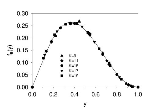
FIG. 1.: The boson structure function $f_{B}$ at various numerical resolutions, with $M=\mu$, $\langle:\!\!\phi^{2}(0)\!\!:\rangle=1$, $\Lambda^{2}=50\mu^{2}$, and $\mu_{1}^{2}=10\mu^{2}$. The solid line is the parameterized fit, $Ay^{a}(1-y)^{b}$.

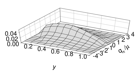
FIG. 2.: The one-boson amplitude $\phi^{(1,0)}$ as a function of longitudinal momentum fraction $y$ and one transverse momentum component $q_{x}$ in the $q_{y}=0$ plane. The parameter values are $K=21$, $N_{\perp}=7$, $\mu_{1}^{2}=10\mu^{2}$, $\Lambda^{2}=25\mu^{2}$, and $\langle:\!\!\phi^{2}(0)\!\!:\rangle=1$.

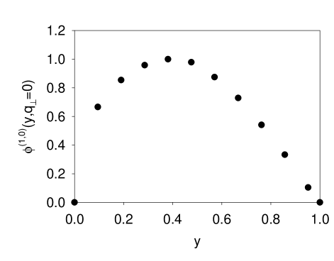
FIG. 3.: The boson-fermion two-body amplitude at zero transverse momentum, with $K=21$, $N_{\perp}=7$, $\langle:\!\!\phi^{2}(0)\!\!:\rangle=1$, $\Lambda^{2}=25\mu^{2}$, and $\mu_{1}^{2}=10\mu^{2}$. The normalization is arbitrary.

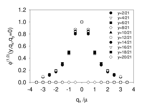
FIG. 4.: Cross sections of the boson-fermion two-body amplitude taken at varying longitudinal momenta and at fixed $q_{y}=0$, with $K=21$, $N_{\perp}=7$, $\langle:\!\!\phi^{2}(0)\!\!:\rangle=1$, $\Lambda^{2}=25\mu^{2}$, and $\mu_{1}^{2}=10\mu^{2}$. The peaks are normalized to be equal at $q_{x}=0$.

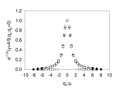
FIG. 5.: A cross section of the boson-fermion two-body amplitude taken at fixed longitudinal momentum fraction $y=4/9$ and at fixed $q_{y}=0$, with $K=9$, $\langle:\!\!\phi^{2}(0)\!\!:\rangle=1$, and $\mu_{1}^{2}=10\mu^{2}$. The cutoff $\Lambda^{2}$ and the transverse resolution $N_{\perp}$ are varied to keep the transverse scale $L_{\perp}$ fixed at one of the following values: $1\frac{\pi}{\mu}$ (black), $\sqrt{2}\frac{\pi}{\mu}$ (gray), and $2\frac{\pi}{\mu}$ (white). Different symbol shapes correspond to different values of $N_{\perp}$. The peaks are normalized to be equal at $q_{x}=0$. The points at zero amplitude mark the transverse range, which is set by the cutoff.

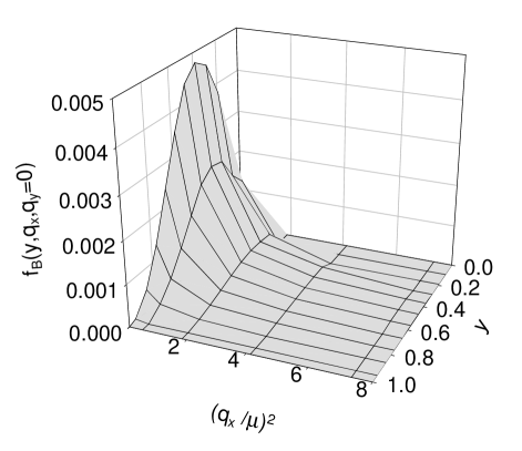
FIG. 6.: The boson structure function $f_{B}(y,{\bf q}_{\perp})$ with $K=21$, $N_{\perp}=7$, $\langle:\!\!\phi^{2}(0)\!\!:\rangle=1$, $\Lambda^{2}=25\mu^{2}$, and $\mu_{1}^{2}=10\mu^{2}$. The transverse momentum is varied with $q_{y}$ fixed at zero.

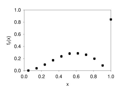
FIG. 7.: The fermion structure function $f_{F}$ with $K=21$, $N_{\perp}=5$ to 7, $\langle:\!\!\phi^{2}(0)\!\!:\rangle=1$, $\Lambda^{2}=25\mu^{2}$, and $\mu_{1}^{2}=10\mu^{2}$. Each $N_{\perp}$ value yields essentially the same result.

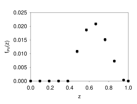
FIG. 8.: Same as Fig. 7 but for the Pauli–Villars boson structure function $f_{PV}$.

Other values for the physical parameters $M$ and $\langle:\!\!\phi^{2}(0)\!\!:\rangle$ have also been considered. A summary of extrapolated quantities is given in Table IV. The associated structure functions $f_{B}(y)$ are shown in Figs. 9 through 12. Distribution amplitudes are displayed in Figs. 13 and 14. For values of $M$ larger than $\mu$ we have found the form $Ay^{a}(1-y)^{b}e^{-cy}$ to allow a noticeably better fit to $f_{B}(y)$. For $\langle:\!\!\phi^{2}(0)\!\!:\rangle=5$ the maximum number of bosons was increased to 5. The numerical resolutions ranged from 9 to 21 for $K$ and from 5 to as much as 10 for $N_{\perp}$.

The extent to which the fermion source is dressed by the bosons is directly determined by the mass ratio $M/\mu$ and the coupling strength. The latter is tightly correlated with the chosen observable $\langle:\!\!\phi^{2}(0)\!\!:\rangle$. As the ratio $M/\mu$ is tuned, the boson structure function $f_{B}(y)$ shifts dramatically. A relatively small boson mass shifts the peak in $f_{B}(y_{)}$ to small boson momentum fractions, as shown in Fig. 11. A large mass shifts the peak to central values of $y$ and significantly raises the constituent density at large $y$, as illustrated in Fig. 9. An increase in $\langle:\!\!\phi^{2}(0)\!\!:\rangle$ increases the coupling and increases the probability for a large number of constituents. Analogous changes occur for the distribution amplitude. Comparison of Tables III and IV shows that the average number $\langle n_{B}\rangle$ increases significantly when $\langle:\!\!\phi^{2}(0)\!\!:\rangle$ is changed from 1 to 5.

TABLE IV.: Same as Table III, but for different $M^{2}$ or $\langle:\!\!\phi^{2}(0)\!\!:\rangle$ values.

	$\langle:\!\!\phi^{2}(0)\!\!:\rangle=1$			$\langle:\!\!\phi^{2}(0)\!\!:\rangle=5$
$(M/\mu)^{2}$	0.1	5	10	1
$(\mu_{1}/\mu)^{2}$	10	10	10	10
$(\Lambda/\mu)^{2}$	50	100	100	50
$g/\mu$	15.1	18.1	19.0	44.5
$M^{\prime}_{0}/\mu^{2}$	1.39	1.66	1.60	10.1
$|\psi_{0}|^{2}$	0.83	0.89	0.90	0.41
$-100\mu^{2}\tilde{F}^{\prime}(0)$	2.0	0.14	0.07	6.7
$\langle n_{B}\rangle$	0.16	0.10	0.09	0.62
$\langle y\rangle$	0.073	0.032	0.024	0.24
$\langle y_{1}y_{2}\rangle_{n\geq 2}-\langle y\rangle_{n\geq 2}^{2}$	$7\cdot 10^{-4}$	$3\cdot 10^{-4}$	$3\cdot 10^{-4}$	$8\cdot 10^{-3}$
$A$	1.0333	5.2548	7.5519	9.0847
$a$	1.0512	1.3191	1.3339	1.0256
$b$	0.8678	2.5430	1.7151	2.1580
$c$	0	2.2730	4.9870	0

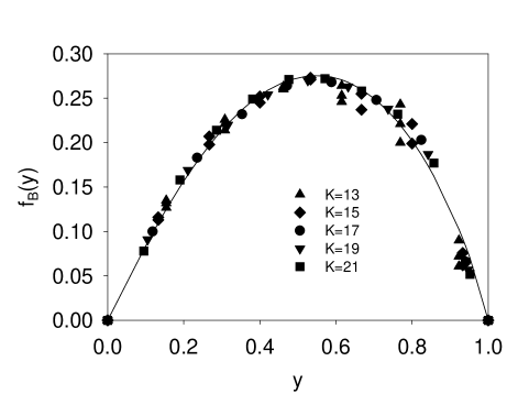
FIG. 9.: Same as Fig. 1, but for $M^{2}=0.1\mu^{2}$.

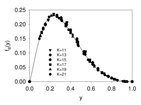
FIG. 10.: Same as Fig. 1, but for $M^{2}=5\mu^{2}$ and $\Lambda=100\mu^{2}$ and a parameterized fit of $Ay^{a}(1-y)^{b}e^{-cy}$.

FIG. 11.: Same as Fig. 10, but for $M^{2}=10\mu^{2}$.

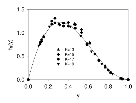
FIG. 12.: Same as Fig. 1, but for $\langle:\!\!\phi^{2}(0)\!\!:\rangle=5$.

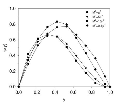
FIG. 13.: Comparison of distribution amplitudes $\varphi(y)\equiv\int d^{2}q_{\perp}\phi^{(1,0)}(y,\mathchoice{{\hbox{\boldmath$\displaystyle q$}}}{{\hbox{\boldmath$\textstyle q$}}}{{\hbox{\boldmath$\scriptstyle q$}}}{{\hbox{\boldmath$\scriptscriptstyle q$}}}_{\perp})$. Various values are considered for the fermion mass $M$, with $\langle:\!\!\phi^{2}(0)\!\!:\rangle=1$. The values of the numerical parameters are $K=19$, $N_{\perp}=5$, $\Lambda^{2}=50\mu^{2}$ (except for $M^{2}=5\mu^{2}$ and $10\mu^{2}$ when $\Lambda^{2}=100\mu^{2}$), and $\mu_{1}^{2}=10\mu^{2}$. The lines simply connect the computed points, to guide the eye, and the absolute normalization is arbitrary.

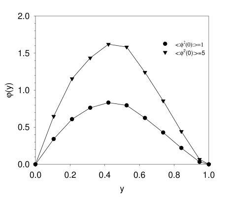
FIG. 14.: Same as Fig. 13 but with the fermion mass fixed at $M=\mu$ and $\langle:\!\!\phi^{2}(0)\!\!:\rangle$ varied.

IV Conclusion

We have successfully computed the Fock-sector wave functions which fully describe the lowest-mass eigenstate of a field-theoretic model Hamiltonian (4) in physical three space and one time dimensions. From these wave functions we have extracted several interesting quantities to show that numerical convergence is under control and that Pauli–Villars regularization leads to sensible results. The size of the momentum-state basis required is large but manageable for present-day computing machines. Larger bases could be used by expanding to more than one node, although one then pays the price of message-passing overhead.

For the model discussed here there are still interesting calculations which might be done. One could look at excited states in the one-fermion sector that we have explored, or consider other sectors, such as the two-fermion sector. Extension to two flavors, particularly with very different masses, should yield some understanding of light systems with heavy intrinsic constituents, which could have some relevance for intrinsic charm[21].

Beyond this model there are, of course, many possibilities. A solution of Yukawa theory[22], in a no-pair approximation or eventually in full, would be the most immediate nontrivial extension. Applications to quantum electrodynamics, to positronium[10] or the electron’s anomalous moment[11] in particular, would be quite natural. Direct application to quantum chromodynamics (QCD) may be problematic; however, a supersymmetric conformally-invariant form of QCD could lend itself to the spirit of the approach, in that heavy superpartners in a broken supersymmetry should provide the needed ultraviolet cancellations.

REFERENCES

• [1] K.G. Wilson, Phys. Rev. D10, 2445 (1974).
• [2] M. Neubert, Report No. hep-ph/9812396, submitted to J. High Energy Phys., 1998; M. Suzuki, Phys. Rev. D 58, 111504 (1998); Report No. hep-ph/9901327. For a description of the difficulties found in computing needed final state interactions in lattice gauge theory, see L. Maiani and M. Tesla, Phys. Lett. B 245, 585 (1990); C. Michael, Nucl. Phys. B 327, 515 (1989).
• [3] W.A. Bardeen and R. Pearson, Phys. Rev. D 14, 547 (1976); W.A. Bardeen, R.B. Pearson, and E. Rabinovici, ibid21, 1037 (1980); P.A. Griffin, Mod. Phys. Lett. A 7, 601 (1992); Nucl. Phys. B372, 270 (1992); Phys. Rev. D 46, 3538 (1992); 47, 3530 (1993); M. Burkardt, ibid47, 4628 (1993); 49, 5446 (1994); M. Burkardt, in the proceedings of the 1995 ELFE Summer School and Workshop, Confinement Physics, edited by S. Bass and P.A.M. Guichon, (Gif-sur-Yvette, Ed. Frontieres, 1996), p. 255; M. Burkardt and B. Klindworth, Phys. Rev. D 55, 1001 (1997); S. Dalley and B. van de Sande, hep-th/9806231.
• [4] For reviews, see S.J. Brodsky and H.-C. Pauli, in Recent Aspects of Quantum Fields, edited by H. Mitter and H. Gausterer, Lecture Notes in Physics Vol. 396 (Springer-Verlag, Berlin, 1991); S.J. Brodsky, G. McCartor, H.-C. Pauli, and S.S. Pinsky, Part. World 3, 109 (1993); M. Burkardt, Adv. Nucl. Phys. 23, 1 (1996); S.J. Brodsky, H.-C. Pauli, and S.S. Pinsky, Phys. Rep. 301, 299 (1997) hep-ph/9705477.
• [5] S.J. Brodsky, J.R. Hiller, G. McCartor, Phys. Rev. D 58, 025005 (1998).
• [6] H.-C. Pauli and S.J. Brodsky, Phys. Rev. D 32, 1993 (1985); 32, 2001 (1985).
• [7] W. Pauli and F. Villars, Rev. Mod. Phys. 21, 4334 (1949).
• [8] K.G. Wilson, T.S. Walhout, A. Harindranath, W.-M. Zhang, R.J. Perry, and St.D. Głazek, Phys. Rev. D 49, 6720 (1994); St.D. Głazek and K.G. Wilson, Phys. Rev. D 48, 5863 (1993); 49, 4214 (1994); M. Brisudová and R.J. Perry, Phys. Rev. D 54, 1831 (1996); M. Brisudová and R.J. Perry, ibid54, 6453 (1996); M. Brisudová, R.J. Perry, and K.G. Wilson, Phys. Rev. Lett. 78, 1227 (1997); B.D. Jones, R.J. Perry, and St.D. Głazek, Phys. Rev. D 55, 6561 (1997); B.D. Jones and R.J. Perry, ibid., 7715 (1997). See also K. Harada and A. Okazaki, ibid., 6198 (1997); E.L. Gubankova and F. Wegner, Phys. Rev. D 58, 025012 (1998).
• [9] L.C.L. Hollenberg, K. Higashijima, R.C. Warner and B.H.J. McKellar, Prog. Th. Phys. 87, 441 (1992).
• [10] A.C. Tang, Ph.D. thesis, SLAC Report No. 351, 1990; A.C. Tang, S.J. Brodsky, and H.-C. Pauli, Phys. Rev. D 44, 1842 (1991); M. Kaluža and H.-C. Pauli, Phys. Rev. D 45, 2968 (1992); M. Krautgärtner, H.C. Pauli, and F. Wölz, ibid45, 3755 (1992); M. Kaluža and H.J. Pirner, ibid47, 1620 (1993); H.C. Pauli and J. Merkel, ibid55, 2486 (1997); U. Trittmann and H.-C. Pauli, Report No. hep-th/9704215 (unpublished); Report No. hep-th/9705021 (unpublished); U. Trittmann, Report No. hep-th/9705072 (unpublished); Report No. hep-th/9706055 (unpublished).
• [11] J.R. Hiller and S.J. Brodsky, Phys. Rev. D 59, 016006 (1999).
• [12] J.J. Wivoda and J.R. Hiller, Phys. Rev. D 47, 4647 (1993).
• [13] I. Tamm, J. Phys. (Moscow) 9, 449 (1945); S.M. Dancoff, Phys. Rev. 78, 382 (1950).
• [14] P.A.M. Dirac, Rev. Mod. Phys. 21, 392 (1949).
• [15] G. McCartor and D.G. Robertson, Z. Phys. C 53, 679 (1992).
• [16] G.P. Lepage and S.J. Brodsky, Phys. Rev. D 22, 2157 (1980).
• [17] C. Lanczos, J. Res. Nat. Bur. Stand. 45, 255 (1950); J.H. Wilkinson, The Algebraic Eigenvalue Problem (Clarendon, Oxford, 1965); B.N. Parlett, The Symmetric Eigenvalue Problem (Prentice–Hall, Englewood Cliffs, NJ, 1980); J. Cullum and R.A. Willoughby, J. Comput. Phys. 44, 329 (1981); Lanczos Algorithms for Large Symmetric Eigenvalue Computations (Birkhauser, Boston, 1985), Vol. I and II; G.H. Golub and C.F. van Loan, Matrix Computations (Johns Hopkins University Press, Baltimore, 1983).
• [18] J. Cullum and R.A. Willoughby, in Large-Scale Eigenvalue Problems, eds. J. Cullum and R.A. Willoughby, Math. Stud. 127 (Elsevier, Amsterdam, 1986), p. 193.
• [19] P.L. DeVries, A First Course in Computational Physics, (Wiley, New York, 1994), pp. 72-73.
• [20] St.D. Głazek and R.J. Perry, Phys. Rev. D 45, 3734 (1992).
• [21] S.J. Brodsky, P. Hoyer, C. Peterson and N. Sakai, Phys. Lett. 93B, 451 (1980). R. Vogt and S.J. Brodsky, Nucl. Phys. B438, 261 (1995) hep-ph/9405236.
• [22] For a light-cone bound-state calculation in Yukawa theory, using basis-function methods, see St. Głazek, A. Harindranath, S. Pinsky, J. Shigemitsu, and K. Wilson, Phys. Rev. D 47, 1599 (1993); P.M. Wort, ibid47, 608 (1993).