CERN-TH/99-71

Saclay-T99/026

hep-ph/9903389

A Boltzmann Equation for the QCD Plasma
Jean-Paul BLAIZOT

Service de Physique Théorique, CE-Saclay
91191 Gif-sur-Yvette, France and

Edmond IANCU

Theory Division, CERN
CH-1211, Geneva 23, Switzerland

We present a derivation of a Boltzmann equation for the QCD plasma, starting from the quantum field equations. The derivation is based on a gauge covariant gradient expansion which takes consistently into account all possible dependences on the gauge coupling assumed to be small. We point out a limitation of the gradient expansion arising when the range of the interactions becomes comparable with that of the space-time inhomogeneities of the system. The method is first applied to the case of scalar electrodynamics, and then to the description of long wavelength colour fluctuations in the QCD plasma. In the latter case, we recover Bödecker’s effective theory and its recent reformulation by Arnold, Son and Yaffe. We discuss interesting cancellations among various collision terms, which occur in the calculation of most transport coefficients, but not in that of the quasiparticle lifetime, or in that of the relaxation time of colour excitations.

CERN-TH/99-71

March 1999

Published in Nuclear Physics B 557 (1999) 183-236.

1 Introduction

At high temperature, non-Abelian gauge theories describe weakly coupled plasmas whose constituents, quarks and gluons for hot QCD, have typical momenta $k\sim T$, where $T$ is the temperature [1, 2, 3]. The plasma particles may take part in collective excitations which develop typically on a space-time scale $\lambda\sim 1/gT$ much larger than the mean interparticle distance $\bar{r}\sim 1/T$ ($g$ is the gauge coupling, assumed to be small). Such collective excitations can be described in terms of mean fields carrying appropriate quantum numbers and coupled to the plasma particles. In this long-wavelength limit, the plasma particles obey simple, collisionless, kinetic equations which can be viewed as the generalization of the Vlasov equation of ordinary plasmas [4, 5, 1].

In this paper, we shall be interested in specific collective excitations involving colour fluctuations on larger wavelengths, $\lambda\sim 1/g^{2}T$. In this situation, the effects of the collisions among the plasma particles become as important as those of the mean fields. The kinetic equations obeyed by the plasma particles must therefore be generalized so as to include the collisions terms. This is what we shall do here. The Boltzmann equation that we shall obtain (see eqs. (1.1)—(1.3) below) turns out to be identical to the one proposed recently by Arnold, Son and Yaffe [7], and yields, in leading logarithmic accuracy, Bödeker’s effective theory for the soft ($p\sim g^{2}T$) fields [6]. The derivation presented here, starting from the quantum field equations, clarifies the nature of the approximations involved, and thus fixes its range of applicability. Furthermore, it also provides some justification for numerous previous works using ad hoc transport equations inspired by classical transport theory [8, 9, 10, 11, 12, 13, 14, 15, 16]. It should be emphasized that transport equations with a similar colour structure have been also proposed in Refs. [17, 10], and that some of the technics that we shall be using have been used already by many authors [18, 19, 20, 21, 22]. However, in most of these works, the organizing role of the various dynamical scales which appear in hot QCD was not recognized, which led to unecessarily complicated, and sometimes inconsistent, equations.

In fact, “kinetic theory” in the way we use it here could be regarded as a powerful tool for constructing effective theories for the soft modes of the plasma. These soft degrees of freeedom are represented by mean fields, while the hard ones, which are “integrated out” using perturbation theory, survive as induced sources for these mean fields. The resulting effective theory can then be studied non-perturbatively, e.g., as a classical theory on a lattice: recently, this strategy has received much attention in connection with studies of baryon number violation in the high temperature electroweak theory [23, 24, 25, 26, 6, 7, 27, 16]. Let us also recall that this method has been first demonstrated for the collective dynamics at the scale $gT$, where we have shown [4, 5] that simple, collisionless, kinetic equations resum an infinite number of one-loop diagrams with soft external lines and hard loop momenta, the so-called “hard thermal loops” [28, 29].

Let us now summarize the main equations to be obtained below. The collective, longwavelength colour fluctuations of the hard transverse gluons are described by a density matrix $N({\bf k},x)$ which, to the order of interest, can be written in the form:

$$N_{ab}({\bf k},x)\,=\,N(\varepsilon_{k})\delta_{ab}-gW_{ab}(x,{\bf v})\,({\rm d}N/{\rm d}\varepsilon_{k}),$$ (1.1)

where $N(\varepsilon_{k})\equiv 1/({\rm e}^{\beta\varepsilon_{k}}-1)$ is the Bose-Einstein thermal distribution (with $\varepsilon_{k}=|{\bf k}|$), and the function $W(x,{\bf v})$, which parametrizes the off-equilibrium deviation, is a colour matrix in the adjoint representation, $W(x,{\bf v})\equiv W_{a}(x,{\bf v})T^{a}$, which depends upon the velocity ${\bf v}={\bf k}/\varepsilon_{k}$ (a unit vector), but not upon the magnitude $k\equiv|{\bf k}|$ of the momentum. The functions $W_{a}(x,{\bf v})$ satisfy the following transport equation:

$$(v\cdot D_{x})^{ab}W_{b}(x,{\bf v}) = {\bf v}\cdot{\bf E}^{a}(x)-\gamma\left\{W^{a}(x,{\bf v})-{\left\langle\Phi({\bf v\cdot v}^{\prime})W^{a}(x,{\bf v}^{\prime})\right\rangle\over\left\langle\Phi({\bf v\cdot v}^{\prime})\right\rangle}\right\}.$$ (1.2)

In the left hand side of this equation, $v\cdot D_{x}$ is a gauge-covariant drift operator (with $v^{\mu}\equiv(1,{\bf v})$ and $D^{\mu}\equiv\partial^{\mu}+igA^{\mu}$), while in the right hand side we recognize a mean field term (${\bf v}\cdot{\bf E}^{a}(x)$, with ${\bf E}^{a}$ the chromoelectric field) and a collision term. The latter is proportional to the quasiparticle damping rate $\gamma$, which appears to set the scale for the colour relaxation time: $\tau_{col}\sim 1/\gamma\sim 1/(g^{2}T\ln(1/g))$ (see below). The other notations above are as follows: the angular brackets in the collision term denote angular average over the directions of the unit vector ${\bf v}^{\prime}$ (as in eq. (1.4) below), and the quantity $\Phi({\bf v\cdot v}^{\prime})$ is given by:

$$\Phi({\bf v\cdot v}^{\prime})\equiv(2\pi)^{2}\int{{\rm d}^{4}q\over(2\pi)^{4}}\,\delta(q_{0}-{\bf q\cdot v})\delta(q_{0}-{\bf q\cdot v}^{\prime})\Big{|}{}^{*}{\cal D}_{l}(q)+({\bf v}_{t}\cdot{\bf v}_{t}^{\prime})\,{}^{*}{\cal D}_{t}(q)\Big{|}^{2}.\,\,\,$$ (1.3)

where ${}^{*}{\cal D}_{l}(q)$ and ${}^{*}{\cal D}_{t}(q)$ denote the resummed gluon propagators in the electric and the magnetic channels, respectively [1, 2]. Up to a normalization, $\Phi({\bf v\cdot v}^{\prime})$ is the total interaction rate for two hard particles with momenta ${\bf k}$ and ${\bf p}$ (and velocities ${\bf v}\equiv\hat{\bf k}$ and ${\bf v}^{\prime}\equiv\hat{\bf p}$) in the (resummed) Born approximation, as illustrated in Fig. 1 (${\bf v}_{t}$ and ${\bf v}_{t}^{\prime}$ are the transverse projections of the velocities with respect to the momentum ${\bf q}$ of the exchanged gluon: e.g., $v_{t}^{i}=(\delta^{ij}-\hat{q}^{i}\hat{q}^{j})v^{j}$). The damping rate $\gamma$ is obtained from $\Phi({\bf v\cdot v}^{\prime})$ as follows:

$$\gamma\,=\,{g^{4}N_{c}^{2}T^{3}\over 6}\int{{\rm d}\Omega^{\prime}\over 4\pi}\,\Phi({\bf v\cdot v}^{\prime})\,\simeq\,{g^{2}N_{c}T\over 4\pi}\ln(1/g),$$ (1.4)

and is of O$(g^{2}T)$ in spite of the explicit factor $g^{4}$ in front of the above integral. This is because the quasiparticle damping is dominated by soft momentum transfers $q\mathrel{\hbox to0.0pt{\raise 2.20013pt\hbox{$<$}\hss}{\lower 2.20013pt\hbox{$\sim$}}}gT$, which gives an enhancement factor $\sim 1/g^{2}$ after the resummation of the screening effects at the scale $gT$ [28, 30, 31, 32].

Actually, in the present approximation, $\gamma$ is even logarithmically infrared divergent, due to the unscreened static ($q_{0}\to 0$) magnetic interactions. (In writing the right hand side of eq. (1.4) we have assumed an infrared cutoff $\sim g^{2}T$, as it is usually done in the literature [31, 10, 12].) To logarithmic accuracy, that is, by preserving only the singular piece of the magnetic scattering element in eq. (1.3) (see eq. (3.123) below), eqs. (1.2)–(1.3) generate Bödeker’s effective theory for the soft modes $A^{\mu}_{a}$ [6].

Figure 1: Elastic scattering in the (resummed) Born approximation. The continuous lines refer to hard gluons (these are off-equilibrium propagators), while the wavy line is the soft gluon exchanged in the collision. The blob stands for HTL resummation.

Within the same accuracy, eq. (1.2) can be solved to get the so-called colour conductivity [10, 12, 6, 7]. The induced colour current is expressed in terms of $W(x,{\bf v})$ as:

$${\bf j}^{a}(x)\,=\,m_{D}^{2}\langle{\,\bf v}\,W^{a}(x,{\bf v})\rangle,$$ (1.5)

with the Debye mass $m_{D}^{2}=g^{2}N_{c}T^{2}/3$. For constant colour electric fields, we get from eq. (1.2):

$$W^{a}({\bf v})\,=\,{1\over\gamma}\,{\bf v}\cdot{\bf E}^{a},$$ (1.6)

so that

$${\bf j}^{a}\,=\,{m_{D}^{2}\over 3\gamma}\,{\bf E}^{a}\,\equiv\,\sigma_{c}{\bf E}^{a},$$ (1.7)

with the colour conductivity $\sigma_{c}=m_{D}^{2}/3\gamma\sim T/\ln(1/g)$.

The next section of the paper contains a derivation of the Boltzmann equation for scalar electrodynamics (SQED). There are several reasons for this. First, to our knowledge, this is the first consistent derivation of a Boltzmann equation for gauge theories, starting form the quantum field equations. Second, it serves as a preparation for the more involved non Abelian case of QCD which is presented in the following section. Finally, and this is the most important, it will reveal interesting compensations which occur in Abelian, but not in non-Abelian gauge theories. Thus, in SQED, most transport phenomena are dominated by large angle scattering, so that the typical relaxation times are $\tau_{tr}\sim 1/(e^{4}T\ln(1/e))$, where $e$ is the electric charge [9, 15]. This is to be contrasted with the quasiparticle lifetimes which are limited by small angle scatterings and are of order $\tau\sim 1/(g^{2}T\ln(1/g))$ (in both QED and QCD). The same cancellations occur in most cases for QCD as well (thus yielding, e.g., a viscous relaxation time $\tau_{visc}\sim 1/(g^{4}T\ln(1/g))$ [9, 14]), except for the the relaxation of colour excitations which remains dominated by very soft gluon exchanges [10, 12, 6, 7]. As a result, the colour relaxation time turns out to be of the same order as the quasiparticle lifetime, as is evident in eq. (1.2). This yields a colour conductivity $\sigma_{c}\sim T/\ln(1/g)$, to be contrasted with the usual, electric conductivity: $\sigma_{el}\sim T/(e^{2}\ln(1/e))$ [15].

The main part of the paper is section 3, which contains the derivation of the Boltzmann equation for the QCD plasma, and a discussion of the approximations which are needed in this derivation. These involve a gradient expansion of the Dyson-Schwinger equations, supplemented by a perturbative evaluation of the collision terms and a linearization with respect to the off-equilibrium fluctuations. All these approximations are commonly used in deriving kinetic equations from quantum field theories, and they are generally seen as independent approximations (to some extent they remain so in the case of SQED discussed in Sec. 2 below). However, in order to fulfill the constraints imposed by a non Abelian gauge symmetry, we shall see that it is convenient to control all these approximations by the same small parameter, namely the gauge coupling $g$. Thus, for instance, the amplitudes of the mean fields will be restricted so that $|A_{a}^{\mu}|\sim gT\,$: this guarantees that the two terms in the soft covariant derivative $D_{X}^{\mu}=\partial_{X}^{\mu}+igA^{\mu}$ are of the same order in $g$, $\partial_{X}\sim gA\sim g^{2}T$, so that $D_{X}={\rm O}(g^{2}T)$ can be preserved consistently in the expansion. A further difficulty that we shall have to face is related to the poor convergence of the gradient expansion when the range of the interactions becomes comparable to the scale of the system inhomogeneities. As we shall see this will be the main limitation of the accuracy of the collision term.

For completeness, we present in section 4 some diagrammatic interpretation of the Boltzmann equation. (Previously, the connection between Feynman graphs and the Boltzmann equation has been explored in detail only for a scalar field theory, in Refs. [33, 34].) The section 5 summarizes the conclusions.

2 Scalar QED

In this section, we briefly summarize the general formalism which allows one to construct kinetic equations from the Dyson-Schwinger equations obeyed by the non-equilibrium Green’s functions [35, 36, 37, 38, 39, 40, 41]. In order to bring out the essential aspects of the formalism while avoiding the complications specific to non Abelian gauge theories, we shall consider here scalar electrodynamics (SQED), with Lagrangian:

$${\cal L} = (D_{\mu}\phi)(D^{\mu}\phi)^{*}-{1\over 4}F_{\mu\nu}F^{\mu\nu},$$ (2.1)

where $\phi$ is a complex scalar field, $A_{\mu}$ is the photon field, $D_{\mu}\equiv\partial_{\mu}+ieA_{\mu}$ is a covariant derivative, and $F_{\mu\nu}$ the field strength tensor, $F_{\mu\nu}=\partial_{\mu}A_{\nu}-\partial_{\nu}A_{\mu}$.

The systems that we consider are assumed to be initially in thermal equilibrium, and described by the density operator $\rho={1\over Z}\exp\left\{-\beta H\right\}$ where $H$ is the Hamiltonian corresponding to (2.1), and $Z$ is the partition function. At some time $t_{0}$, a time-dependent external perturbation (an electromagnetic current $j_{\mu}(x)$) starts acting on the system, so that the Hamiltonian becomes:

$$H_{j}(t)\,=\,H\,+\,\int{\rm d}^{3}{x}\,j(t,{\bf x})\cdot A({\bf x})\,,$$ (2.2)

where $j\cdot A=j_{\mu}\,A^{\mu}$. The density operator at time $t$ is given by:

$${\rho}(t)\,=\,U(t,t_{0})\,\rho\,U(t_{0},t),$$ (2.3)

where $U(t,t_{0})$, the evolution operator, satisfies:

$$i\partial_{t}\,U(t,t_{0})\,=\,H_{j}(t)U(t,t_{0}),\qquad\qquad U(t_{0},t_{0})\,=\,1.$$ (2.4)

In the presence of the perturbation, the gauge field $A^{\mu}$ develops an expectation value:

$${\rm Tr}\Bigl{(}\rho(t)A^{\mu}\Bigr{)}\,=\,{\rm Tr}\Bigl{(}\rho\,A^{\mu}(t)\Bigr{)}\,=\,{\rm Tr}\left\{{{\rm e}^{-\beta H}\over Z}\,A^{\mu}(t)\right\}\equiv\,\langle A^{\mu}(t)\rangle\,,$$ (2.5)

with

$$A^{\mu}(t)\equiv U^{-1}(t,t_{0})\,A^{\mu}\,U(t,t_{0})\,=\,U(t_{0},t)\,A^{\mu}\,U(t,t_{0}),$$ (2.6)

where we have used the fact that $U(t_{0},t)=U^{-1}(t,t_{0})$. More generally, we shall be interested in various $n$-point functions, and in particular in 2-point functions for which we shall derive equations of motion in the next subsection. For instance, the time-ordered 2-point function of the charged scalar field is given by:

$$G(t_{1},t_{2}) = \langle{\rm T}\,\phi(t_{1})\phi^{\dagger}(t_{2})\rangle\equiv{\rm Tr}\left\{{{\rm e}^{-\beta H}\over Z}\,{\rm T}\,\phi(t_{1})\phi^{\dagger}(t_{2})\right\},\$$ (2.7)

$$= \theta(t_{1}-t_{2})G^{>}(t_{1},t_{2})+\theta(t_{2}-t_{1})G^{<}(t_{1},t_{2})$$

where $\phi(t)=U(t_{0},t)\,\phi\,U(t,t_{0})$, and the functions $G^{>}$ and $G^{<}$ are defined by:

$$G^{>}(x,y)\,\equiv\,\langle\phi(x)\phi^{\dagger}(y)\rangle,\qquad G^{<}(x,y)\,\equiv\,\langle\phi^{\dagger}(y)\phi(x)\rangle.$$ (2.8)

(To lighten the notation, the spatial coordinates have not been indicated in eq. (2.7).) The functions $G^{>}$ and $G^{<}$ can be used to construct the retarded $(G_{R})$ and advanced $(G_{A})$ propagators, which will also be needed:

$$G_{R}(x,y) \equiv i\theta(x_{0}-y_{0})\Bigl{[}G^{>}(x,y)\,-\,G^{<}(x,y)\Bigr{]}\,,$$

$$G_{A}(x,y) \equiv -i\theta(y_{0}-x_{0})\Bigl{[}G^{>}(x,y)\,-\,G^{<}(x,y)\Bigr{]}\,.$$ (2.9)

Similar definitions hold for the photon 2-point functions. In the case of the photon, we shall decompose the gauge field into its average value for which we shall reserve the notation $A_{\mu}(x)$ (i.e., in the following we identify $\langle A_{\mu}\rangle\to A_{\mu}$), and a fluctuating part $a_{\mu}(x)$ with $\langle a_{\mu}\rangle=0$. The time ordered photon propagator is then given by:

$${\cal D}_{\mu\nu}(x,y)=\langle{\rm T}a_{\mu}(x)a_{\nu}(y)\rangle.$$ (2.10)

The 2-point functions introduced above satisfy boundary conditions which follow from their definitions (cf. eq. (2.7)). For instance:

$$G^{<}(t_{0},z)\,=\,G^{>}(t_{0}-i\beta,z),$$ (2.11)

and similarly for the photon 2-point functions and for the various self-energies to be introduced later. Furthermore, these functions have hermiticity properties which will be useful below. Specifically, all the “bigger” ($>$) and “lesser” ($<$) 2-point functions are hermitian: for instance, $(G^{>}(x,y))^{*}=G^{>}(y,x)$ and $({\cal D}^{>}_{\mu\nu}(x,y))^{*}={\cal D}^{>}_{\nu\mu}(y,x)$. This, together with the definitions (2), imply $(G_{R}(x,y))^{*}=G_{A}(y,x)$ and $({\cal D}^{\mu\nu}_{R}(x,y))^{*}={\cal D}^{\nu\mu}_{A}(y,x)$, together with similar properties for the various self-energies.

In thermal equilibrium, the system is homogeneous (e.g., $G^{<}_{eq}(x,y)\equiv G^{<}_{eq}(x-y)$), and it is convenient to go to momentum space. Then, the boundary condition (2.11) translates into the so-called KMS condition [2] :

$$G^{>}_{eq}(k) = {\rm e}^{\beta k_{0}}G^{<}_{eq}(k),$$ (2.12)

which implies the following structure for the equilibrium 2-point functions:

$$G^{>}_{eq}(k)=\rho(k)\Bigl{[}1+N(k_{0})\Bigr{]},\,\,\qquad\,\,G^{<}_{eq}(k)=\rho(k)\,N(k_{0})\,,$$ (2.13)

with $N(k_{0})\equiv 1/({\rm e}^{\beta k_{0}}-1)$ and the spectral density $\rho(k)\equiv G^{>}_{eq}(k)-G^{<}_{eq}(k)$. In particular, for free, massless particles:

$$G^{<}_{0}(k)\equiv\rho_{0}(k)N(k_{0}),\qquad G^{>}_{0}(k)\equiv\rho_{0}(k)[1+N(k_{0})],$$ (2.14)

with $\rho_{0}(k)=2\pi\epsilon(k_{0})\delta(k^{2})$.

2.1 Equations of motion for Green’s functions

Figure 2: Complex-time contour for the evaluation of the thermal expectation values: $C=C_{+}\cup C_{-}\cup C_{0}$.

In order to obtain the equations of motion for the 2-point functions, it is convenient to extend their definition by allowing the time variables to take complex values. More specifically, we introduce, in the complex time plane, the oriented contour depicted in Fig. 2. This may be seen as the juxtaposition of three pieces: $C=C_{+}\cup C_{-}\cup C_{0}$. We call $z$ the (complex) time variable along the contour, and reserve the notation $t$ for real times. On $C_{+}$, $z=t$ takes all the real values between $t_{0}$ to $t_{f}$. On $C_{-}$, we set $z=t-i\eta$ ($\eta\to 0_{+}$) and $t$ runs backward from $t_{f}$ to $t_{0}$. Finally, on $C_{0}$, $z=t_{0}-i\tau$, with $0<\tau\leq\beta$. We define a contour $\theta$-function $\theta_{C}$: $\theta_{C}(z_{1},z_{2})=1$ if $z_{1}$ is further than $z_{2}$ along the contour (we then write $z_{1}\succ z_{2}$), while $\theta_{C}(z_{1},z_{2})=0$ if the opposite situation holds ($z_{1}\prec z_{2}$). We can formalize this by introducing a real parameter $u$ which is continously increasing along the contour; then, the contour $C$ is specified by a function $z(u)$, and $\theta_{C}(z_{1},z_{2})=\theta(u_{1}-u_{2})$. We shall later need also a contour delta function, which we define by:

$$\delta_{C}(z_{1},z_{2})\equiv\left({\partial z\over\partial u}\right)^{-1}\delta(u_{1}-u_{2}).$$ (2.15)

The definition of the propagators is then extended in a natural way. For instance, the contour-ordered propagator of the scalar field becomes:

$$G(z_{1},z_{2})\,\equiv\,\langle{\rm T}_{C}\,\phi(z_{1})\phi^{\dagger}(z_{2})\rangle\equiv{\rm Tr}\left\{{{\rm e}^{-\beta H}\over Z}\,{\rm T}_{C}\,\phi(z_{1})\phi^{\dagger}(z_{2})\right\},$$ (2.16)

where ${\rm T}_{C}$ orders the operators on its right, from right to left in increasing order of the arguments $u_{i}$. For time arguments $t_{1}$, $t_{2}$ on $C_{+}$, the contour propagator (2.16) reduces to the time-ordered propagator (2.7). For $t_{1}\in C_{-}$ and $t_{2}\in C_{+}$, we have $G(t_{1}-i\eta,t_{2})\,=\,G^{>}(t_{1},t_{2})$, while for $t_{1}\in C_{+}$ and $t_{2}\in C_{-}$, we have $G(t_{1},t_{2}-i\eta)\,=\,G^{<}(t_{1},t_{2})$.

With these definitions in hand, most of the formal manipulations familiar in equilibrium field theory can be extended to the case of non equilibrium. This is convenient for the derivation of the equations of motion for the $n$-point functions to which we now turn.

The mean field equation is:

$$\partial_{\nu}F^{\mu\nu}(x)=j^{\mu}(x)+j^{\mu}_{ind}(x),$$ (2.17)

with the induced current

$$j^{\mu}_{ind}(x)=-ie\Bigl{\langle}\left(D^{\mu}\phi(x)\right)^{\dagger}\phi(x)\,-\phi^{\dagger}(x)\left(D^{\mu}\phi(x)\right)\Bigr{\rangle}.$$ (2.18)

In this expression, $D_{\mu}=\partial_{\mu}+ig(A_{\mu}+a_{\mu})$. However, in line with the approximations below, we can ignore the contribution of the quantum field $a_{\mu}$ in the expression of the induced current. This amounts to neglect the contribution of a connected 3-point function. We can then write:

$$j^{\mu}_{ind}(x)=ie\left(D^{\mu}_{x}-\left(D^{\mu}_{y}\right)^{\dagger}\right)\left.G^{<}(x,y)\right|_{x=y},$$ (2.19)

where now, and for the rest of this section, $D_{\mu}=\partial_{\mu}+igA_{\mu}$, with $A_{\mu}$ the average gauge potential.

In order to calculate the induced current, we need the 2-point function $G^{<}(x,y)$. An equation of motion for this function can be obtained from the equation of motion for the time ordered propagator:

$$-D^{2}_{x}\,G(x,y)\,-\,i\int_{C}{\rm d}^{4}z\,\Sigma(x,z)\,G(z,y)\,=\,i\delta_{C}(x,y),$$ (2.20)

where $\delta_{C}(x_{0},y_{0})$ is the contour delta function, and $\Sigma$ the scalar self-energy. The latter admits the following decomposition, similar to that of $G$, eq. (2.7):

$$\Sigma(x,y)\,=\,-i\hat{\Sigma}(x)\delta_{C}(x,y)\,+\,\theta_{C}(x_{0},y_{0})\Sigma^{>}(x,y)+\theta_{C}(y_{0},x_{0})\Sigma^{<}(x,y).$$ (2.21)

We have separated out a possible singular piece $\hat{\Sigma}$ (e.g., the standard tadpole diagram which generates a temperature-dependent mass correction [42]). The non-singular components $\Sigma^{>}$ and $\Sigma^{<}$ obey a boundary condition similar to (2.11). In particular, in equilibrium, $\Sigma^{>}_{eq}(k)={\rm e}^{\beta k_{0}}\Sigma^{<}_{eq}(k)$.

The equations of motion in real-time for the mean field and the 2-point functions are obtained by letting the external time variables $x_{0}$ and $y_{0}$ take values on the real-time pieces of this contour, $C_{+}$ and $C_{-}$. For $x_{0}\in C_{+}$, the mean field equation is formally the same as in eq. (2.17). Consider now eq. (2.20): by choosing $x_{0}\in C_{+}$ and $y_{0}\in C_{-}$, and by using the decompositions (2.7) and (2.21), we obtain, after some manipulations, an equation for $G^{<}(x,y)$:

$$\Bigl{(}D^{2}_{x}+\hat{\Sigma}(x)\Bigr{)}G^{<}(x,y)\,=\,-\int{\rm d}^{4}z\,\Bigl{[}\Sigma_{R}(x,z)\,G^{<}(z,y)\,+\,\Sigma^{<}(x,z)\,G_{A}(z,y)\Bigr{]},$$

(2.22)

together with a similar equation where the differential operator is acting on $y$:

$$\Bigl{(}(D^{\dagger}_{y})^{2}+\hat{\Sigma}(y)\Bigr{)}G^{<}(x,y)\,=\,-\int{\rm d}^{4}z\,\Bigl{[}G^{<}(x,z)\,\Sigma_{A}(z,y)\,+\,G_{R}(x,z)\,\Sigma^{<}(z,y)\Bigr{]}.$$

(2.23)

In these equations, $D^{2}=D^{\mu}D_{\mu}$, $D_{\mu}^{\dagger}=\partial_{\mu}-ieA_{\mu}$, and we have used the definitions (2) for the retarded and advanced Green’s functions, together with similar definitions for $\Sigma_{R}$ and $\Sigma_{A}$. One can also obtain an equation satisfied by $G_{R}(x,y)$:

$$\Bigl{(}D^{2}_{x}+\hat{\Sigma}(x)\Bigr{)}G_{R}(x,y)\,+\,\int{\rm d}^{4}z\,\Sigma_{R}(x,z)\,G_{R}(z,y)\,=\,\delta^{(4)}(x-y)\,.$$ (2.24)

Note that, while the Green’s functions $G^{>}$ and the $G^{<}$ and the corresponding self-energies are coupled by eqs. (2.1)–(2.1), the retarded Green’s function $G_{R}$ is determined by the retarded self-energy $\Sigma_{R}$ alone.

The above equations must be supplemented with some approximation scheme in which, for instance, the self-energy $\Sigma$ is expressed in terms of the propagator $G$. Below, we shall use perturbation theory for this purpose. We shall refer to the above equations as the Kadanoff-Baym equations. They were first obtained in the framework of non-relativistic many-body theory [35]. Note that, in these equations, any explicit reference to the initial conditions and to the KMS condition has disappeared. These only enter as boundary conditions to be satisfied by the various Green’s functions in the remote past. The same set of equations has been derived by Keldysh [38] to describe non-equilibrium evolutions of quantum systems (see also [36, 37, 39, 40]).

2.2 Gauge covariant Wigner transforms

For slowly varying off-equilibrium perturbations, the Kadanoff-Baym equations can be transformed into kinetic equations, as we now explain. In thermal equilibrium, the system is homogenous, and the two-point functions depend only on the relative coordinates $s^{\mu}=x^{\mu}-y^{\mu}$. The thermal particles have typical energies and momenta $k\sim T$. It follows that the 2-point functions are peaked around $s^{\mu}=0$, their range of variation being fixed by the thermal wavelength $\lambda_{T}=1/k\sim 1/T$. In what follows, we shall be interested in off-equilibrium deviations which are slowly varying in space and time, over a typical scale $\lambda\gg\lambda_{T}$.

In order to take advantage of the assumed separation of scales between hard degrees of freedom (the plasma particles), and the soft degrees of freedom (the collective excitations at scale $\lambda\gg\lambda_{T}$), it is convenient to introduce relative and central coordinates,

$$s^{\mu}\equiv x^{\mu}-y^{\mu},\qquad\qquad X^{\mu}\equiv{x^{\mu}+y^{\mu}\over 2}\,,$$ (2.25)

and to use the Wigner transforms of the 2-point functions. These are defined as Fourier transforms with respect to the relative coordinates $s^{\mu}$. For instance, the Wigner transform of $G^{<}(x,y)$ is:

$$G^{<}(k,X)\equiv\int{\rm d}^{4}s\,{\rm e}^{ik\cdot s}\,G^{<}\left(X+{s\over 2},X-{s\over 2}\right),$$ (2.26)

and we shall use similar definitions for the other 2-point functions. Note that we shall use the same symbols for the 2-point functions and their Wigner transforms, considering that the different functions can be recognized from their arguments.

The hermiticity properties of the 2-point functions discussed after eq. (2.11) imply similar properties for the corresponding Wigner functions. For instance, from $(G^{>}(x,y))^{*}=G^{>}(y,x)$ we deduce that $G^{<}(k,X)$ is a real function, $(G^{<}(k,X))^{*}=G^{<}(k,X)$, and similarly for $G^{>}(k,X)$. Also, $(G_{A}(k,X))^{*}=G_{R}(k,X)$. Similar properties hold for the photon 2-point functions and for the various self-energies.

In gauge theories, the physical interpretation of the Wigner functions as phase space densities is complicated by the lack of gauge covariance of the 2-point functions. To remedy this, we shall define new, gauge invariant, functions, whose construction may be motivated by considering the conserved electromagnetic current:

$$j^{\mu}(x)=ie\left(D^{\mu}_{x}-\left(D^{\mu}_{y}\right)^{\dagger}\right)\left.G^{<}(x,y)\right|_{x=y},$$ (2.27)

where $G^{<}(x,y)=\langle\phi^{\dagger}(y)\phi(x)\rangle$ is not gauge invariant. It is easy to define a corresponding gauge invariant function by multiplying it by a parallel transporter, or “Wilson line”,

$$U(x,y)={\rm e}^{-ie\int_{\gamma}{\rm d}z^{\mu}A_{\mu}(z)},$$ (2.28)

where the path $\gamma$ joining $y$ to $x$ is a priori arbitrary. Thus, for instance,

$$\acute{G}^{<}(x,y)\equiv\langle\phi^{\dagger}(y)U(y,x)\phi(x)\rangle=U(y,x)G^{<}(x,y)$$ (2.29)

is manifestly gauge invariant. The conserved current may then be expressed in terms of this gauge invariant function:

$$j^{\mu}(x) = \left(\partial^{\mu}_{x}-\partial^{\mu}_{y}\right)\left.\acute{G}^{<}(x,y)\right|_{x=y}$$ (2.30)

$$= 2i\partial_{s}^{\mu}\left.\acute{G}^{<}(s,X)\right|_{s=0}\,.$$

To see this, note that $G^{<}(x,y)=U(x,y)\acute{G}^{<}(x,y)$, and that $D^{\mu}_{x}\left.U(x,y)\right|_{x=y}=0$. Note also that the expression for $j^{\mu}(x)$ is independent of the path joining $x$ and $y$, since only an infinitesimal path is needed.

For definitness, we shall in fact choose $\gamma$ to be the straight line joining $x$ and $y$. This choice is physically motivated since, as we shall see later, the hard particles preserve straight line trajectories in the presence of the soft mean fields (at least, to leading order in $e$). Moreover, as shown in Refs. [18, 19, 21], such a path allows one to interpret the covariantization procedure as the replacement of the canonical momentum by the kinetic one (see eq. (2.32) below). This being said, most of our results below will be independent of the exact form of $\gamma$ (see, however, the discussion after eq. (2.41)). Indeed, we shall mostly need the parallel transporter $U(x,y)$ in situations where the end points $x$ and $y$ are close to each other ($|s|\mathrel{\hbox to0.0pt{\raise 2.20013pt\hbox{$<$}\hss}{\lower 2.20013pt\hbox{$\sim$}}}1/T$, with $s\equiv x-y$), so that the variation of the field can be neglected along the path. This is a good approximation provided $\gamma$ never goes too far away from $x$ and $y$, that is, provided $|z-X|={\rm O}(1/T)$ (with $X\equiv(x+y)/2$) for any point $z$ on $\gamma$. For any such a path we can write:

$$U\left(x,y\right)\,\approx\,{\rm e}^{\,-ies\cdot A(X)}\,,$$ (2.31)

up to terms which involve, at least, one soft derivative $\partial_{X}A^{\mu}$ (and which do depend upon the path).

Starting from $\acute{G}^{<}(x,y)$, we construct the gauge invariant Wigner function:

$$\acute{G}^{<}(k,X) \equiv \int{\rm d}^{4}s\,{\rm e}^{ik\cdot s}\,U\left(X-{s\over 2},X+{s\over 2}\right)\,G^{<}\left(X+{s\over 2},X-{s\over 2}\right)$$ (2.32)

$$\approx \int{\rm d}^{4}s\,{\rm e}^{\,is\cdot(k+eA(X))}\,G^{<}\left(X+{s\over 2},X-{s\over 2}\right)$$

$$= G^{<}(p=k+eA(X),X).$$

This formula shows that, as alluded to before, the gauge invariant Wigner function may be obtained from the ordinary one by the simple replacement of the canonical momentum $p^{\mu}$ by the kinetic momentum $k^{\mu}=p^{\mu}-eA^{\mu}(X)$. Returning to the current, we see that it takes the form:

$$j^{\mu}(x) = 2e\int{{\rm d}^{4}p\over(2\pi)^{4}}\,\left(p^{\mu}-eA^{\mu}(X)\right)G^{<}(p,X)\,$$ (2.33)

$$= 2e\int{{\rm d}^{4}k\over(2\pi)^{4}}\,k^{\mu}\,\acute{G}^{<}(k,X).$$

These two expressions for the current may be seen as the analogs of eqs. (2.27) and (2.30).

2.3 Gradient expansion and kinetic equations

For slowly varying disturbances, taking place over a scale $\lambda\gg\lambda_{T}$, we expect the $s^{\mu}$ dependence of the 2-point functions to be close to that in equilibrium. Thus, typically, $k\sim\partial_{s}\sim T$, while $\partial_{X}\sim 1/\lambda\ll T$. The general equations of motion written down in Sec. 2.1 can then be simplified with the help of a gradient expansion, using $k$ and $X$ as most convenient variables.

The starting point of the gradient expansion is the equation obtained by taking the difference of the Kadanoff-Baym equations (2.1) and (2.1). For further reference, we shall call it the difference equation. We then define:

$$\Xi(x,y)\equiv D^{2}_{x}-\,(D^{\dagger}_{y})^{2},$$ (2.34)

where:

$$D_{x}^{2} = \partial_{x}^{2}+2ieA(x)\cdot\partial_{x}+ie(\partial\cdot A(x))-e^{2}A^{2}(x),$$

$$(D^{\dagger}_{y})^{2} = \partial_{y}^{2}-2ieA(y)\cdot\partial_{y}-ie(\partial\cdot A(y))-e^{2}A^{2}(y).$$ (2.35)

By replacing the coordinates $x^{\mu}$ and $y^{\mu}$ by $s^{\mu}$ and $X^{\mu}$ (cf. eq. (2.25)), and rewriting the derivatives as:

$$\partial_{x}=\partial_{s}+{1\over 2}\partial_{X},\qquad\,\,\partial_{y}=-\partial_{s}+{1\over 2}\partial_{X}\qquad\,\,\partial_{x}^{2}-\partial_{y}^{2}=2\partial_{s}\cdot\partial_{X},$$ (2.36)

we perform a gradient expansion in $\Xi$, with $\partial_{s}\sim T$ and $\partial_{X}\sim 1/\lambda\ll T$, and preserve all the terms involving at most one soft derivative $\partial_{X}$. For instance,

$$A_{\mu}(X+s/2)\approx A_{\mu}(X)+(1/2)(s\cdot\partial_{X})A_{\mu}(X).$$

A straightforward calculation yields then:

$$\Xi(s,X)\approx 2\,\partial_{s}\cdot\partial_{X}+2ieA_{\mu}(X)\partial^{\mu}_{X}+2ie(s\cdot\partial_{X}A_{\mu})\partial^{\mu}_{s}+2ie(\partial_{X}\cdot A)-e^{2}(s\cdot\partial_{X}A^{2})+\cdots,$$

(2.37)

where the dots stand for terms which involve at least two soft derivatives $\partial_{X}$.

Before taking the Wigner transform, we make the difference equation covariant by multiplying both sides by the parallel transport $U(y,x)$ (cf. eq. (2.29)). For the left hand side, we use the expansion (2.3) of $\Xi(s,X)$, together with eq. (2.31) to obtain:

$$U(y,x)\left(D^{2}_{x}-(D^{\dagger}_{y})^{2}\right)\left(U(x,y)\acute{G}^{<}(x,y)\right)\approx 2\Bigl{(}\partial_{s}\cdot\partial_{X}+ies^{\mu}F_{\mu\nu}(X)\partial_{s}^{\nu}\Bigr{)}\acute{G}^{<}(s,X).$$ (2.38)

The right hand side of the difference equation involves convolutions of the form:

$$C(x,y)\equiv\int{\rm d}^{4}z\,\Sigma(x,z)\,G(z,y).$$ (2.39)

Upon multiplication by $U(y,x)$, this becomes the gauge invariant quantity:

$$\acute{C}(x,y) = U(y,x)\int{\rm d}^{4}z\,U(x,z)\acute{\Sigma}(x,z)U(z,y)\acute{G}(z,y)$$ (2.40)

$$= \int{\rm d}^{4}z\,P(x,y,z)\,\acute{\Sigma}(x,z)\acute{G}(z,y),$$

where we have set $\acute{C}(x,y)\equiv U(y,x)C(x,y)$, and $P(x,y,z)$ denotes the following plaquette:

$$P(x,y,z)\equiv U(y,x)U(x,z)U(z,y).$$ (2.41)

In line with the approximations in eq. (2.38), we need the gradient expansion of eqs. (2.40) and (2.41) up to terms involving one soft derivative of the background field. In each of the parallel transporters, we choose the path $\gamma$ to be the straight line (cf. the discussion before eq. (2.31)). Then, the plaquette (2.41) can be easily expanded around the point $X=(x+y)/2$ to yield:

$$P(x,y,z)\approx\exp\left\{-\,{ie\over 4}s^{\mu}F_{\mu\nu}(X)\delta^{\nu}\right\}\,\approx\,1\,-\,{ie\over 4}s^{\mu}F_{\mu\nu}(X)\delta^{\nu},$$ (2.42)

where $s\equiv x-y$, $X\equiv(x+y)/2$, $\delta\equiv 2(z-X)$.

We are now in position to take the Wigner transform. The only delicate step concerns the transformation of $\acute{C}(x,y)$, which is given by:

$$\acute{C}(k,X)\approx\acute{\Sigma}(k,X)\acute{G}(k,X)+\,{i\over 2}\,\Bigl{\{}\acute{\Sigma},\,\acute{G}\Bigr{\}}_{P.B.}-{i\over 2}eF_{\mu\nu}(X)\left(\partial^{\mu}_{k}\acute{\Sigma}\right)\left(\partial_{k}^{\nu}\acute{G}\right)\,+\,...\,,$$ (2.43)

where $\{A,B\}_{P.B.}$ denotes a Poisson bracket:

$$\Bigl{\{}A,\,{B}\Bigr{\}}_{P.B.}\equiv\partial_{k}A\cdot\partial_{X}{B}\,-\,\partial_{X}A\cdot\partial_{k}{B}\,.$$ (2.44)

The third term in the r.h.s. of eq. (2.43), involving $F_{\mu\nu}(X)$, comes from the plaquette (2.42) and is therefore sensitive to the choice of $\gamma$. To the accuracy where this term is important, we expect the gauge-invariant Wigner functions $\acute{\Sigma}(k,X)$ and $\acute{G}(k,X)$ to be path-dependent as well. However, such path-dependent terms will disappear in the final form of the Boltzmann equation that we shall obtain (see eq. (2.56) below).

By using eqs. (2.38) and (2.43), the difference equation finally becomes:

$$2(k\cdot\partial_{X}-ek\cdot F\cdot\partial_{k})\acute{G}^{<} + (\partial_{X}^{\mu}\hat{\Sigma})\partial_{\mu}^{k}\acute{G}^{<}-\left\{{\rm Re}\acute{\Sigma}_{R},\acute{G}^{<}\right\}_{P.B.}-\left\{\acute{\Sigma}^{<},{\rm Re}\acute{G}_{R}\right\}_{P.B.}$$ (2.45)

$$+ eF^{\mu\nu}\left((\partial_{\mu}^{k}\acute{\Sigma}^{<})(\partial_{\nu}^{k}{\rm Re}\acute{G}_{R})+(\partial_{\mu}^{k}{\rm Re}\acute{\Sigma}_{R})(\partial_{\nu}^{k}\acute{G}^{<})\right)$$

$$= -\left(\acute{G}^{>}\acute{\Sigma}^{<}-\acute{\Sigma}^{>}\acute{G}^{<}\right)$$

In deriving the equation above, we have used the following relations:

$$\acute{G}_{R}(k,X)-\acute{G}_{A}(k,X) = i\Bigl{(}\acute{G}^{>}(k,X)-\acute{G}^{<}(k,X)\Bigr{)}\,\equiv\,i\rho(k,X),$$

$$\acute{\Sigma}_{R}(k,X)-\acute{\Sigma}_{A}(k,X) = i\Bigl{(}\acute{\Sigma}^{>}(k,X)-\acute{\Sigma}^{<}(k,X)\Bigr{)}\,\equiv\,-i\Gamma(k,X),$$ (2.46)

which follow, e.g., from the definitions (2) for $G_{R}$ and $G_{A}$ after multiplying with $U(y,x)$ and taking the Wigner transform. Note that the right hand sides of eqs. (2.3) define two new Wigner functions, $\rho(k,X)$ and $\Gamma(k,X)$, which are real quantities (cf. the discussion after eq. (2.26)) and can be seen as off-equilibrium generalizations of the corresponding spectral densities in equilibrium (recall eq. (2.13)). In terms of these functions we have, for instance:

$$\acute{G}_{R}(k,X)=\int_{-\infty}^{\infty}{{\rm d}k_{0}^{\prime}\over 2\pi}\,{\rho(k_{0}^{\prime},{\bf k},X)\over k_{0}^{\prime}-k_{0}-i\eta}\,,\qquad\acute{\Sigma}_{R}(k,X)=-\int_{-\infty}^{\infty}{{\rm d}k_{0}^{\prime}\over 2\pi}\,{{\Gamma}(k_{0}^{\prime},{\bf k},X)\over k_{0}^{\prime}-k_{0}-i\eta}\,.$$ (2.47)

Eq. (2.45) also involves:

$$2{\rm Re}\,\acute{G}_{R}\,=\,\acute{G}_{R}+\acute{G}_{A},\qquad 2{\rm Re}\,\acute{\Sigma}_{R}(k,X)\,=\,\acute{\Sigma}_{R}+\acute{\Sigma}_{A}.\,\,$$ (2.48)

Further manipulations allow us to put eq. (2.45) in the form:

$$(2k-\partial_{k}{\rm Re}\acute{\Sigma})\cdot({\rm d}_{X}\,\acute{G}^{<}) + (\partial_{X}{\rm Re}\acute{\Sigma})\cdot(\partial_{k}\acute{G}^{<})$$ (2.49)

$$- (\partial_{k}\acute{\Sigma}^{<})\cdot({\rm d}_{X}\,{\rm Re}\acute{G}_{R})+(\partial_{X}\acute{\Sigma}^{<})\cdot(\partial_{k}{\rm Re}\acute{G}_{R})$$

$$= -\left(\acute{G}^{>}\acute{\Sigma}^{<}-\acute{\Sigma}^{>}\acute{G}^{<}\right),$$

where ${\rm Re}\,\acute{\Sigma}\equiv{\rm Re}\,\acute{\Sigma}_{R}+\hat{\Sigma}$, and ${\rm d}_{X}^{\mu}\equiv\partial_{X}^{\mu}-eF^{\mu\nu}(X)\partial_{\nu}^{k}$. It is interesting to note that the corresponding equation for a scalar field theory (like $\lambda\phi^{4}$) can be obtained by simply replacing ${\rm d}_{X}^{\mu}$ by $\partial_{X}^{\mu}$ in the above equation [3].

In equilibrium, both sides of eq. (2.49) are identically zero. This is obvious for the terms in the l.h.s., which involve the soft derivative $\partial_{X}$ or mean field insertions, and can be easily verified for the terms in the r.h.s. by using the KMS conditions for $G_{eq}$ and $\Sigma_{eq}$ (cf. eq. (2.12)). Thus, eq. (2.49) is a transport equation which describes the space-time evolution of long-wavelength fluctuations in the average density of the charged particles. It holds to leading order in the gradient expansion (that is, up to terms involving at least two powers of the soft derivative), and to all orders in the interaction coupling strength.

To conclude this section, note that, within the previous approximations (that is, up to terms involving at least two soft derivatives), the retarded propagator $\acute{G}_{R}(k,X)$ satisfies an equation which is formally identical to that it obeys in equilibrium:

$$\Bigl{(}k^{2}-\hat{\Sigma}(X)-\acute{\Sigma}_{R}(k,X)\Bigr{)}\,\acute{G}_{R}(k,X)\,=\,-1\,.$$ (2.50)

In order to obtain this equation, start with eq. (2.24) for $G_{R}(x,y)$ together with its conjugate equation where the differential operator acts on $y$; then, consider the sum of these two equations, and perform a gauge-invariant gradient expansion as above. In this expansion, all the terms involving one soft derivative $\partial_{X}$ cancel, and the same holds also for the terms involving the soft mean field. From eqs. (2.47) and (2.50), we deduce an expression for the off-equilibrium spectral density:

$$\rho(k,X)\,=\,2\,{\rm Im}\,\acute{G}_{R}(k,X)\,=\,{\Gamma(k,X)\over\Bigl{(}k^{2}-{\rm Re}\,\acute{\Sigma}(k,X)\Bigr{)}^{2}\,+\,\Bigl{(}\Gamma(k,X)/2\Bigr{)}^{2}}\,,$$ (2.51)

which will be useful in discussing the quasiparticle approximation below.

2.4 Mean-field and quasiparticle approximations

In order to make progress with eq. (2.49) further approximations are needed. In particular, we shall use below perturbation theory to express the self-energies $\acute{\Sigma}^{<}$ and $\acute{\Sigma}^{>}$ in terms of the propagators $\acute{G}^{<}$ and $\acute{G}^{>}$. As a first step, let us consider the mean field approximation in which the self energies $\acute{\Sigma}$ are neglected altogether. The equation (2.49) reduces then to $(k\cdot{\rm d}_{X})\acute{G}^{<}(k,X)=0$, or, more explicitly:

$$\left(k\cdot\partial_{X}-ek_{\mu}F^{\mu\nu}(X)\partial_{\nu}^{k}\right)\acute{G}^{<}(k,X)=0.$$ (2.52)

This equation describes the motion of independent particles in the mean field $F_{\mu\nu}$. In this approximation the spectral density remains the same as in the free theory in equilibrium, as obvious from eq. (2.51): $\rho(k,X)\approx\rho_{0}(k)\equiv 2\pi\epsilon(k_{0})\delta(k^{2})N(k_{0})$. Accordingly, the solution to eq. (2.52) can be written in the form:

$$\acute{G}^{<}(k,X)=2\pi\delta(k^{2})\Bigl{\{}\theta(k_{0})N_{+}({\bf k},X)+\theta(-k_{0})(1+N_{-}(-{\bf k},X))\Bigr{\}},$$ (2.53)

where the density matrices $N_{\pm}({\bf k},X)$ satisfy the Vlasov equation [39]:

$$\Bigl{(}v\cdot\partial_{X}\,\pm\,e({\bf E+v\times B})\cdot\mbox{\boldmath$\nabla$}_{k}\Bigr{)}N_{\pm}({\bf k},X)=0,$$ (2.54)

with $v^{\mu}=(1,{\bf v})$ and ${\bf v}=\hat{\bf k}$ is the velocity of the charged particle. The density matrices $N_{\pm}({\bf k},X)$ may be given the interpretation of classical phase-space distributions for particles and antiparticles. In terms of them, the induced current is simply:

$$j^{\mu}(x) = e\int{{\rm d}^{3}k\over(2\pi)^{3}}\,v^{\mu}\,\Bigl{(}N_{+}({\bf k},X)\,-\,N_{-}({\bf k},X)\Bigr{)}.$$ (2.55)

Going beyond the mean field approximation, we need to take into account the various effects of the self-energies. We shall concentrate here on a commonly used approximation which consists in neglecting the broadening of the single-particle states when computing the collision terms, an approximation which we refer to as the “quasiparticle approximation”. Indeed, the interaction rate $\Gamma$ in eq. (2.51) is of higher order in $e$ (specifically, $\Gamma\sim(e^{2}\ln(1/e))T^{2}$, as we shall see below), so we can use the mean field spectral density, $\rho(k,X)\approx\rho_{0}(k)$, to estimate the collision terms. At the same time, we shall ignore the self-energy terms in the l.h.s. of eq. (2.49). That this is consistent can be verified by power counting (we shall do this explicitly for the QCD case, in Sec. 3.5); it is also physically motivated from the fact that the role of these terms is to account for the difference between $\rho(k,X)$ and $\rho_{0}(k)$ in the transport equation for $\acute{G}^{<}(k,X)$ [3]. Thus, in the quasiparticle approximation, the Wigner functions $\acute{G}^{<}(k,X)$ and $\acute{G}^{>}(k,X)$ preserve the same on-shell structure as in the mean field approximation, as displayed in eq. (2.53).

We thus end up with the following kinetic equation:

$$2\left(k\cdot\partial_{X}-ek_{\mu}F^{\mu\nu}(X)\partial_{\nu}^{k}\right)\acute{G}^{<}(k,X)=-\left(\acute{G}^{>}\acute{\Sigma}^{<}-\acute{\Sigma}^{>}\acute{G}^{<}\right),$$ (2.56)

where, in line with the weak coupling expansion, we choose the self energies $\acute{\Sigma}^{<}$ and $\acute{\Sigma}^{>}$ so as to reproduce the one-photon-exchange scattering in Fig. 1 (Born approximation). As we shall see in the next section, this generates a collision term of the standard Boltzmann form. Note also that eq. (2.56) in independent upon the choice of the path $\gamma$ in eq. (2.28); indeed, the terms which were explicitly path-dependent in eq. (2.49) have disappeared in the approximations leading to eq. (2.56). Moreover, we shall verify shortly that, to the order of interest, the self-energies $\acute{\Sigma}^{<}$ and $\acute{\Sigma}^{>}$ are path-independent as well.

In computing transport coefficients like viscosities or electric conductivity (see, e.g., Refs. [9, 14, 15, 34, 43]), or the quasiparticle damping rate [11, 3], it is only necessary to consider small off-equilibrium deviations, so that the linearized version of eq. (2.56) can be used. We then write, e.g., $\acute{G}^{<}\equiv G^{<}_{eq}+\delta\acute{G}^{<}$ and $\acute{\Sigma}^{<}\equiv\Sigma^{<}_{eq}+\delta\acute{\Sigma}^{<}$ (with $\delta\acute{G}\ll G_{eq}$, $\delta\acute{\Sigma}\ll\Sigma_{eq}$), and linearize the collision term with respect to the small fluctuations $\delta\acute{G}$ and $\delta\acute{\Sigma}\,$:

$$C(k,X) \equiv -\Bigl{(}\acute{G}^{>}(k,X)\acute{\Sigma}^{<}(k,X)-\acute{\Sigma}^{>}(k,X)\acute{G}^{<}(k,X)\Bigr{)}$$ (2.57)

$$\simeq -\Bigl{(}\Sigma^{<}_{eq}\,\delta\acute{G}^{>}-\Sigma^{>}_{eq}\,\delta\acute{G}^{<}\Bigr{)}+\Bigl{(}\delta\acute{\Sigma}^{>}\,G_{eq}^{<}-\delta\acute{\Sigma}^{<}\,G_{eq}^{>}\Bigr{)}.$$

In the quasiparticle approximation, we further have $G_{eq}^{>}\approx G_{0}^{>}$, $G_{eq}^{<}\approx G_{0}^{<}$ and $\delta\acute{G}^{<}\approx\delta\acute{G}^{>}\equiv\delta\acute{G}$ (since $\acute{G}^{>}(k,X)-\acute{G}^{<}(k,X)=\rho_{0}(k)=G^{>}_{0}(k)-G^{<}_{0}(k)$). Then, the linearized collision term takes the form:

$$C(k,X)\simeq-\Gamma_{eq}(k)\,\delta\acute{G}(k,X)\,+\,\Bigl{(}\delta\acute{\Sigma}^{>}\,G_{0}^{<}\,-\,\delta\acute{\Sigma}^{<}\,G_{0}^{>}\Bigr{)},$$ (2.58)

where we have isolated the damping rate in equilibrium (cf. eq. (2.3)):

$$\Gamma_{eq}(k)\,=\,\Sigma^{<}_{eq}(k)-\Sigma^{>}_{eq}(k).$$ (2.59)

Note that the quasiparticle approximation is not a self-consistent approximation, but it is in line with the weak coupling expansion: the collision term generates a width which is not included in the spectral densities which are used to estimate it; however, the neglected terms are of higher order than those we have kept.

The most direct application of the formula above is the calculation of the quasiparticle damping rate [35, 11, 3]. To this aim, we consider a specific off-equilibrium deviation which is obtained by adding, at $t_{0}=0$, a particle with momentum ${\bf p}$ and energy $p_{0}=\varepsilon_{p}\equiv|{\bf p}|$ to a plasma initially in equilibrium. Since, for a large system, this is a small perturbation, we can neglect all mean field effects and assume $N({\bf p},t)$ to be only a function of time (here, $N({\bf p},t)\equiv N_{+}({\bf p},t)$; cf. eq. (2.53)). Moreover, for momenta ${\bf k}\neq{\bf p}$, the distribution function does not change appreciably from the equilibrium value $N(\varepsilon_{k})$, so that, to leading order in the external perturbation, we can ignore the off-equilibrium fluctuations of the self-energies: $\delta\acute{\Sigma}^{<}\approx\delta\acute{\Sigma}^{>}\approx 0$. Then, eqs. (2.53), (2.56) and (2.58) yield a very simple equation for the fluctuation $\delta N({\bf p},t)$ (with $\Gamma({\bf p})\equiv\Gamma_{eq}(p_{0}=\varepsilon_{p},{\bf p})$) :

$$2\varepsilon_{p}{\partial\over\partial t}\delta N({\bf p},t)\,=\,-\Gamma({\bf p})\delta N({\bf p},t),$$ (2.60)

whose solution shows exponential attenuation in time:

$$\delta N({\bf p},t)\,=\,\delta N({\bf p},0)\,{\rm e}^{-2\gamma(p)t}\,.$$ (2.61)

The quasiparticle damping rate $\gamma$ is here conventionally defined as $\gamma(p)\equiv\Gamma({\bf p})/4\varepsilon_{p}$ [2]. (This simple picture is actually complicated by infrared effects to be discussed in Sec. 2.6 [30, 31, 32].)

2.5 The collision terms

Figure 3: The two-loop self-energy diagram which describes collisions in the Born approximation. The wavy lines denote free, equilibrium, photon propagators. The other lines are off-equilibrium scalar propagators.

We now turn to the calculation of the collisional self-energy corresponding to Fig. 1. As it is well known (and will be verified later), the corresponding transport cross section is dominated by relatively hard momentum transfers, $eT\mathrel{\hbox to0.0pt{\raise 2.20013pt\hbox{$<$}\hss}{\lower 2.20013pt\hbox{$\sim$}}}q\mathrel{\hbox to0.0pt{\raise 2.20013pt\hbox{$<$}\hss}{\lower 2.20013pt\hbox{$\sim$}}}T$. When the photon momentum is hard, $q\sim T$, the process in Fig. 1 is described by the two-loop self-energy depicted in Fig. 3 in which all the lines are hard, and the scalar propagators are to be understood as off-equilibrium propagators. The photon propagators, on the other hand, are just free propagators in equilibrium. At soft momenta $q\sim eT$, the relevant self-energy is given by the effective one-loop diagram in Fig. 4 in which both the internal lines denote off-equilibrium propagators; the scalar line is hard, while the photon line is soft and dressed by the off-equilibrium polarization tensor in the one-loop approximation (this is denoted by a blob). That is, the diagram in Fig. 4 involves an infinite series of bubble insertions along the photon line, as illustrated in Fig. 5.

Figure 4: The effective one-loop self-energy which describes collisions in the resummed Born approximation. The blob on the photon line denotes the resummation of the one-loop polarization tensor (cf. Fig. (6)).

Figure 5: One of the multi-loop diagrams (containing $n$ bubble insertions along the photon line) which is included in the effective one-loop diagram in Fig. 4.

It is furthermore convenient to recognize that the diagram in Fig. 3 is one of the family of diagrams displayed in Fig. 5; thus, we can use the effective one-loop self-energy in Fig. 4 to describe the collision in Fig 1 for all photon momenta, which we shall do in what follows. To evaluate this diagram, we need the vertex coupling the photon to the scalar field in the presence of the classical background field $A_{\mu}$. This can be read off the Lagrangian:

$${\cal L} = \left(D^{\dagger}_{\mu}-iea_{\mu}\right)\phi^{\dagger}\left(D^{\mu}+iea^{\mu}\right)\phi$$ (2.62)

$$= iea_{\mu}\left[\left(D_{\mu}\phi\right)^{\dagger}\phi-\phi^{\dagger}\left(D_{\mu}\phi\right)\right]+e^{2}a_{\mu}a^{\mu}\phi^{\dagger}\phi,$$

where $D_{\mu}=\partial_{\mu}+ieA_{\mu}$. There are two relevant vertices: $-2ie\phi^{\dagger}a_{\mu}D^{\mu}\phi$ and $-ie\phi^{\dagger}\phi\partial^{\mu}a_{\mu}$. The self-energy reads then:

$$\Sigma(x,y) = e^{2}\biggl{\{}4\Bigl{(}D_{x}^{\mu}D^{\nu\,\dagger}_{y}G(x,y)\Bigr{)}{\cal D}_{\mu\nu}(x,y)+2\Bigl{(}D^{\mu}_{x}G(x,y)\Bigr{)}\Bigl{(}\partial^{\nu}_{y}{\cal D}_{\mu\nu}(x,y)\Bigr{)}$$ (2.63)

$$\qquad+\,2\Bigl{(}D^{\nu\,\dagger}_{y}G(x,y)\Bigr{)}\Bigl{(}\partial_{x}^{\mu}{\cal D}_{\mu\nu}(x,y)\Bigr{)}+G(x,y)\Bigl{(}\partial^{x}_{\mu}\partial^{\nu}_{y}{\cal D}^{\mu\nu}(x,y)\Bigr{)}\biggr{\}}.$$

Here, ${\cal D}_{\mu\nu}(x,y)$ is the off-equilibrium photon propagator, to be constructed shortly. By appropriately choosing $x_{0}$ and $y_{0}$ along the contour, we get expressions for both $\Sigma^{>}$ and $\Sigma^{<}$. For instance, $\Sigma^{>}(x,y)$ will involve $G^{>}(x,y)$ and $D^{>}(x,y)$, etc. Below, to simplify the notations, the upper indices $>$ and $<$ will be often omitted.

We need then to evaluate the gauge invariant self energy $\acute{\Sigma}(x,y)\equiv U(y,x)\Sigma(x,y)$. In doing that, we meet terms like:

$$U(y,x)\,D^{\mu}_{x}\,G(x,y)=U(y,x)\,D^{\mu}_{x}\left(U(x,y)\acute{G}(x,y)\right).$$ (2.64)

Performing the gradient expansion of such a term, one gets:

$$U(y,x)\,D^{\mu}_{x}\left(U(x,y)\acute{G}(x,y)\right)$$ (2.65)

$$\approx {\rm e}^{ies\cdot A(X)}\left(\partial_{s}^{\mu}+ieA^{\mu}(X)\right)\left\{{\rm e}^{-ies\cdot A(X)}\acute{G}(s,X)\right\}$$

$$\approx \partial^{\mu}_{s}\acute{G}(s,X).$$

Note that, in the above manipulations, we have used the simple approximation (2.31) for $U(x,y)$, which makes the final result independent of the choice the path in the Wilson line. The same holds for all the other results in this section.

Similarly, we get $\partial^{\nu}_{y}{\cal D}_{\mu\nu}(x,y)\approx-\partial^{\nu}_{s}{\cal D}_{\mu\nu}(s,X),$ so that the expression
$D^{\mu}_{x}G(x,y)\partial^{\nu}_{y}{\cal D}_{\mu\nu}(x,y)$ becomes simply $-\partial^{\mu}_{s}\acute{G}(s,X)\partial^{\nu}_{s}{\cal D}_{\mu\nu}(s,X)$. Proceeding in the same way for the other terms, and performing the Wigner transform, we get:

$$\acute{\Sigma}(k,X)\,\approx\,e^{2}\int{{\rm d}^{4}q\over(2\pi)^{4}}\,\left(2k^{\mu}-q^{\mu}\right)\left(2k^{\nu}-q^{\nu}\right)\acute{G}(k-q,X){\cal D}_{\mu\nu}(q,X).$$ (2.66)

This is formally the same expression as in equilibrium, except for the fact that $\acute{G}(k-q,X)$ and ${\cal D}_{\mu\nu}(q,X)$ are off-equilibrium propagators and $k^{\mu}$ has to be interpreted as the kinetic momentum. (Note that the photon propagator ${\cal D}_{\mu\nu}$ does not need a special treatment since it is invariant under the gauge transformations of the background field.)

Figure 6: One-loop contributions to the photon self-energy in SQED. All the internal lines are off-equilibrium propagators.

The photon propagator ${\cal D}_{\mu\nu}(x,y)$ obeys Dyson-Schwinger equations similar to eqs. (2.1)–(2.24). Specifically,

$$\left(g^{\mu\nu}\partial^{2}-\partial^{\mu}\partial^{\nu}-\hat{\Pi}^{\mu\nu}\right)_{x}{\cal D}^{<}_{\nu\rho}(x,y)\,=\,\int{\rm d}^{4}z\,\Bigl{(}\Pi_{R}{\cal D}^{<}+\Pi^{<}{\cal D}_{A}\Bigr{)}^{\mu}_{\,\,\,\rho}(x,y),$$ (2.67)

and similarly:

$$\left(g_{\mu\nu}\partial^{2}-\partial_{\mu}\partial_{\nu}-\hat{\Pi}_{\mu\nu}\right)_{x}{\cal D}_{R}^{\nu\rho}(x,y)\,-\,\int{\rm d}^{4}z\,\Pi^{R}_{\mu\nu}{\cal D}_{R}^{\nu\rho}(x,y)\,=\,\delta_{\mu}^{\rho}\delta^{(4)}(x-y)\,,$$ (2.68)

where, to the order of interest, $\Pi_{\mu\nu}(x,y)$ is given by the one-loop diagrams in Fig. 6. That is, $\hat{\Pi}^{\mu\nu}(x)$ is the tadpole contribution in Fig. 6.b, while the non-local self-energies $\Pi_{R}(x,y)$ and $\Pi^{<}(x,y)$ are determined by the graph in Fig. 6.a. From the equations above, we deduce the following relation between ${\cal D}^{<}$ and $\Pi^{<}$:

$${\cal D}^{<}_{\mu\nu}(x,y)\,=\,-\int{\rm d}^{4}z_{1}{\rm d}^{4}z_{2}\,\,\Bigl{(}{\cal D}_{R}(x,z_{1})\,\Pi^{<}(z_{1},z_{2})\,{\cal D}_{A}(z_{2},y)\Bigr{)}_{\mu\nu},$$ (2.69)

which becomes, after a gradient expansion,

$${\cal D}^{<}_{\mu\nu}(q,X)\,\approx\,-\,\Bigl{(}{\cal D}_{R}(q,X)\,\Pi^{<}(q,X)\,{\cal D}_{A}(q,X)\Bigr{)}_{\mu\nu},$$ (2.70)

up to corrections of O$(\partial_{X}/q)$. Since, as we shall see shortly, the collision terms are saturated by momenta $q\mathrel{\hbox to0.0pt{\raise 2.20013pt\hbox{$>$}\hss}{\lower 2.20013pt\hbox{$\sim$}}}eT$, the corrections to eq. (2.70) are of higher order in $e$ provided $\partial_{X}\mathrel{\hbox to0.0pt{\raise 2.20013pt\hbox{$<$}\hss}{\lower 2.20013pt\hbox{$\sim$}}}e^{2}T$. A similar relation holds between ${\cal D}^{>}(q,X)$ and $\Pi^{>}(q,X)$.

It should be observed here that a new scale is entering the gradient expansion. In most situations before, the soft derivative $\partial_{X}$ appeared in combinations such as $s\cdot\partial_{X}$ with the magnitude of the non-locality $s^{\mu}$ fixed by thermal fluctuations: $s\sim 1/T$. In eq. (2.69), however, the non-localities $x-z_{1}$ or $z_{2}-y$ are of order $1/q$ and may be interpreted as the range of the effective interaction between the colliding particles. Thus, the validity of the gradient expansion in this case relies on the range of this effective interaction being small compared to the scale of the inhomogeneities, as measured by $\partial_{X}^{-1}$. Now, the range of the effective interaction depends on the specific transport processes one is looking at. In most cases, and as a result of cancellations to be exhibited in the next subsection, this range is typically of order $1/T$ (and marginally $1/eT$) so that the gradient expansion is indeed valid to calculate transport coefficients to leading order in $e$ already for processes taking place on a scale $1/e^{2}T$.

To construct the photon self-energy out of equilibrium, we use the interaction vertices from eq. (2.62) and obtain, to the order of interest,

$$\hat{\Pi}_{\mu\nu}(X)=-2g_{\mu\nu}e^{2}\int{{\rm d}^{4}p\over(2\pi)^{4}}\,\acute{G}^{<}(p,X),$$ (2.71)

and (compare to eq. (2.66)) :

$$\Pi_{\mu\nu}^{>}(q,X)\,\approx\,e^{2}\int{{\rm d}^{4}p\over(2\pi)^{4}}\,\left(2p_{\mu}+q_{\mu}\right)\left(2p_{\nu}+q_{\nu}\right)\acute{G}^{>}(p+q,X)\acute{G}^{<}(p,X),$$ (2.72)

together with a similar expression for $\Pi^{<}(q,X)$ which involves $\acute{G}^{<}(p+q,X)$ and $\acute{G}^{>}(p,X)$. These expressions are gauge invariant, as expected. The tadpole piece (2.71) enters the calculation of the retarded propagator ${\cal D}_{R}(q,X)$, which is related to the self-energy $\hat{\Pi}(X)+\Pi_{R}(q,X)$ by the same equation as in equilibrium (cf. eq. (2.50)).

By collecting the previous results, we finally obtain the following collision term:

$$C(k,X)\,=\,-\int{{\rm d}^{4}p\over(2\pi)^{4}}\int{{\rm d}^{4}q\over(2\pi)^{4}}\,\left|{\cal M}_{pk\to p^{\prime}k^{\prime}}\right|^{2}\qquad\qquad$$

$$\times\left\{\acute{G}^{<}(k,X)\acute{G}^{<}(p,X)\acute{G}^{>}(k^{\prime},X)\acute{G}^{>}(p^{\prime},X)-\acute{G}^{>}(k,X)\acute{G}^{>}(p,X)\acute{G}^{<}(k^{\prime},X)\acute{G}^{<}(p^{\prime},X)\right\},$$

where $p^{\prime}=p+q$, $k^{\prime}=k-q$, and ${\cal M}_{pk\to p^{\prime}k^{\prime}}$ is the scattering matrix element:

$$\left|{\cal M}_{pk\to p^{\prime}k^{\prime}}\right|^{2}=e^{4}(k+k^{\prime})^{\mu}(p+p^{\prime})^{\nu}(k+k^{\prime})^{\alpha}(p+p^{\prime})^{\beta}[{\cal D}_{R}(q,X)]_{\mu\nu}[{\cal D}_{A}(q,X)]_{\alpha\beta}\,.$$ (2.74)

This collision term has the standard Boltzmann structure, with a gain term and a loss term. To be in line with the previous approximations, this must be evaluated with the Wigner functions $\acute{G}^{<}$ and $\acute{G}^{>}$ in the quasiparticle approximation, i.e., $\acute{G}^{<}(k,X)$ has the on-shell structure exhibited in eq. (2.53), while $\acute{G}^{>}(k,X)$ reads similarly :

$$\acute{G}^{>}(k,X)=2\pi\delta(k^{2})\Bigl{\{}\theta(k_{0})(1+N_{+}({\bf k},X))+\theta(-k_{0})N_{-}(-{\bf k},X)\Bigr{\}}.$$ (2.75)

Thus, the four energy variables $k_{0},\,p_{0},\,k^{\prime}_{0}$ and $p^{\prime}_{0}$ in eq. (2.5) are always on shell (e.g., $|k_{0}|=\varepsilon_{k}\equiv|{\bf k}|$), but they can be either positive ($k_{0}=\varepsilon_{k}$) or negative ($k_{0}=-\varepsilon_{k}$), corresponding to particles and antiparticles, respectively. Choose $k_{0}>0$ for definitness; then (2.5) describes the $t$-channel particle-particle scattering depicted as Fig. 1 (when all the energy variables are positive), but also the $t$-channel particle-antiparticle scattering (when $k^{\prime}_{0}$ is positive, but $p_{0}$ and $p^{\prime}_{0}$ are both negative), and the particle-antiparticle anihilation (or $s$-channel scattering: $p_{0}$ and $k^{\prime}_{0}$ negative, and $p^{\prime}_{0}$ positive). These various processes are illustrated in Fig. 7.

Figure 7: Scattering processes described by the collision term in eq. (2.5) : (a) particle-particle scattering; (b) particle-antiparticle scattering ($t$-channel); (c) particle-antiparticle annihilation ($s$-channel). In Fig. (c), the virtual photon is always hard, so it needs no resummation.

2.6 Quasiparticle lifetimes vs. relaxation times

At the end of Sec. 2.4, we have seen that the collision term (2.58) yields the quasiparticle lifetime $\tau\sim 1/\gamma$, which is dominated by soft momentum transfers, $q\mathrel{\hbox to0.0pt{\raise 2.20013pt\hbox{$<$}\hss}{\lower 2.20013pt\hbox{$\sim$}}}eT$, and is typically $\tau\sim 1/(e^{2}T\ln(1/e))$ [31, 32]. For transport phenomena, however, it is well known [2, 9, 14, 15] that the Abelian collision term (2.5) is saturated by relatively large momentum transfers $eT\mathrel{\hbox to0.0pt{\raise 2.20013pt\hbox{$<$}\hss}{\lower 2.20013pt\hbox{$\sim$}}}q\mathrel{\hbox to0.0pt{\raise 2.20013pt\hbox{$<$}\hss}{\lower 2.20013pt\hbox{$\sim$}}}T$, and the typical relaxation time for off-equilibrium perturbations is $\tau_{tr}\sim 1/(e^{4}T\ln(1/e))$. The fact that $\tau_{tr}\gg\tau$ is due to specific infrared cancellations in the collision term, that we shall discuss now. Note that in QCD the colour algebra prohibits similar cancellations in the calculation of colour relaxation processes, as we shall see in Secs. 3.8 and 4 below.

Consider then the linearized version of the collision term, as given by eq. (2.58). It is convenient to define (with $\beta=1/T$) :

$$\delta\acute{G}(k,X)\,\equiv\,\rho_{0}(k)\delta N(k,X) \equiv -\rho_{0}(k)W(k,X)\,{{\rm d}N\over{\rm d}k_{0}}$$ (2.76)

$$= \beta\rho_{0}(k)W(k,X)N(k_{0})[1+N(k_{0})]\,$$

where (cf. eq. (2.75)) :

$$\delta N(k,X)\,=\,\theta(k_{0})\delta N_{+}({\bf k},X))-\theta(-k_{0})\delta N_{-}(-{\bf k},X).$$ (2.77)

The function $W(k,X)$ describes the local distorsion of the momentum distribution, as may be seen from the following equation:

$$N(k,X)\,\equiv\,N(k_{0})\,-\,W(k,X)\,{{\rm d}N\over{\rm d}k_{0}}\,\approx\,N(k_{0}-W(k,X)).$$ (2.78)

In terms of these new functions, the linearized collision term takes a particularly simple form,

$$C(k,X) \approx -\beta\rho_{0}(k)\int{\rm d}{\cal T}\,|{\cal M}|^{2}\,N(k_{0})N(p_{0})[1+N(k^{\prime}_{0})][1+N(p^{\prime}_{0})]$$ (2.79)

$$\qquad\,\,\,\,\times\Bigl{\{}W(k,X)+W(p,X)-W(k^{\prime},X)-W(p^{\prime},X)\Bigr{\}},$$

with the following notation for the phase-space integral:

$$\int{\rm d}{\cal T}\,\equiv\,\int{{\rm d}^{4}p\over(2\pi)^{4}}\int{{\rm d}^{4}q\over(2\pi)^{4}}\,\rho_{0}(p)\rho_{0}(p+q)\rho_{0}(k-q).$$ (2.80)

The matrix element $|{\cal M}|^{2}$ in eq. (2.79) is to be computed with the equilibrium retarded and advanced photon propagators ${\cal D}_{R,\,A}(q)$ (cf. eq. (2.74)).

Following eq. (2.58), we identify the damping rate $\Gamma(k)\equiv\Gamma_{eq}(k)$ as the coefficient of $\delta\acute{G}(k,X)$ in the r.h.s. of eq. (2.79), that is, as the term involving the fluctuation $W(k,X)\,$:

$$C_{1}(k,X) = -\beta\rho_{0}(k)W(k,X)\int{\rm d}{\cal T}\,|{\cal M}|^{2}\,N(k_{0})N(p_{0})[1+N(k^{\prime}_{0})][1+N(p^{\prime}_{0})]$$ (2.81)

$$\equiv -\,\Gamma(k)\delta\acute{G}(k,X).$$

One can verify that within the present approximation the above expression of $\Gamma$ satisfies indeed eq. (2.59).

Moreover, in eq. (2.81), $\Gamma(k)$ must be evaluated on the tree-level mass-shell (i.e., at $|k_{0}|=\varepsilon_{k}$), since it is multiplied by the on-shell fluctuation $\delta\acute{G}(k,X)$. This determines the quasiparticle damping rate, $\gamma\equiv(1/4k)\Gamma(k_{0}=k)$, which is, however, well known to be infrared divergent in the present approximation [28, 30, 31, 32]. Specifically, the leading contribution to $\gamma$ comes from soft momenta exchange $q\mathrel{\hbox to0.0pt{\raise 2.20013pt\hbox{$<$}\hss}{\lower 2.20013pt\hbox{$\sim$}}}eT$ in the $t$-channel collisions in Figs. 7.a and b. To evaluate this contribution, we can neglect $q_{0}$ next to $p_{0}$ and $k_{0}$ in the thermal distributions in eq. (2.81), and get:

$$\Gamma(k)\simeq\,\int{\rm d}{\cal T}\,|{\cal M}|^{2}\,N(p_{0})[1+N(p_{0})].$$ (2.82)

To the order of interest, we need the resummed photon propagator in the “hard thermal loop” approximation [1, 2], to be denoted as ${}^{*}{\cal D}_{R}^{\mu\nu}(q)$. This yields (for $q\ll k,\,p$):

$$|{\cal M}|^{2}\,\simeq\,16e^{4}\varepsilon_{k}^{2}\varepsilon_{p}^{2}\,\Big{|}{}^{*}{\cal D}_{l}(q)+({\bf\hat{q}\times v})\cdot({\bf\hat{q}\times v}^{\prime})\,{}^{*}{\cal D}_{t}(q)\Big{|}^{2}.$$ (2.83)

where ${}^{*}{\cal D}_{l}$ and ${}^{*}{\cal D}_{t}$ are the longitudinal (or electric) and the transverse (or magnetic) components of the retarded propagator, with the following IR behaviour (below, $m_{D}$ is the Debye mass, $m_{D}^{2}=e^{2}T^{2}/3$) [1, 2] :

$${}^{*}{\cal D}_{l}(q_{0}\to 0,q)\,\simeq\,{-1\over q^{2}+m_{D}^{2}}\,,\qquad{}^{*}{\cal D}_{t}(q_{0}\ll q)\simeq\,{1\over q^{2}-i\,(\pi q_{0}/4q)\,m_{D}^{2}}\,.$$ (2.84)

Because of Debye screening, the electric contribution to the damping rate $\gamma_{l}$ is finite and of order $e^{4}T^{3}/m_{D}^{2}={\rm O}(e^{2}T)$. In the magnetic sector, the dynamical ($q_{0}\neq 0$) screening [1, 2] is not enough to make finite $\gamma_{t}$, which remains logarithmically divergent (see Ref. [32] for more details):

$$\gamma_{t} \simeq {e^{4}T^{3}\over 24}\,\int{\rm d}q\int_{-q}^{q}{{\rm d}q_{0}\over 2\pi}\,{1\over q^{4}+(\pi m_{D}^{2}q_{0}/4q)^{2}}$$ (2.85)

$$\simeq {e^{2}T\over 4\pi}\,\int_{\mu}^{m_{D}}{{\rm d}q\over q}\,=\,{e^{2}T\over 4\pi}\,\ln{m_{D}\over\mu}\,,$$

where $\mu$ is an IR cutoff and we have retained only the dominant, logarithmically divergent, contribution. The remaining IR divergence in eq. (2.85) is associated to the unscreened static magnetic interactions. Since the latter have an infinite range, one may worry that the gradient expansion may become invalid in the calculation of the damping rate (cf. the remark after eq. (2.70)). Recall, however, that in the calculation of $\gamma$, the particles with which the quasiparticle interacts are in equilibrium, and constitute therefore a uniform background (cf. the discussion at the end of Sec. 2.4.) Thus, the question of the relative sizes of the range of the interaction and that of the space-time inhomogeneities is not an issue here. Rather, the IR divergence in eq. (2.85) is an artifact of the perturbative expansion and can be eliminated by a specific resummation [32] which goes beyond the approximations performed in deriving the Boltzmann equation (see however Ref. [44]).

The IR problem of the damping rate does not show up in the calculation of the transport coefficients, because the IR contribution to $\Gamma$, the first term in the r.h.s. of eq. (2.79), is actually compensated by a similar contribution to the third term, involving $W(k^{\prime},X)\,$: indeed, for soft $q$, $W(k^{\prime},X)\equiv W(k-q,X)\approx W(k,X)$, so that the first and third terms in eq. (2.79) cancel each other. As we shall see in Sec. 4, this can be understood as a cancellation between self-energy and vertex corrections in ordinary Feynman graphs. A similar cancellation occurs between the other two terms in eq. (2.79), namely $W(p,X)$ and $W(p^{\prime},X)$. Thus, in order to see the leading IR ($q\ll T$) behaviour of the full integrand in eq. (2.79), one has to expand $W(k^{\prime},X)$ and $W(p^{\prime},X)$ to higher orders in $q$. This generates extra factors of $q$ which remove the most severe IR divergences in the collision integral. As a result, the typical rate involved in the calculation of the transport coefficients is $\Gamma_{tr}\,\sim\,e^{4}T\ln(1/e)$, where the logarithm originates from screening effects at the scale $eT$.

Of course, the simple arguments above are only good enough to provide an order-of-magnitude estimate for the transport relaxation times. In order to compute transport coefficients, one has to solve the Boltzmann equation (2.56) with the linearized collision term (2.79), which is generally complicated. Explicit solutions can be found, e.g., by using specific Ansätze for the unknown function $W(k,X)$, or by variational methods. Some calculations of this kind can be found in Refs. [9, 14, 15, 33, 34].

3 Boltzmann equation for hot QCD

We now come to the case of the high temperature Yang-Mills plasma. As mentioned in the Introduction, we are interested in the regime of ultrasoft colour excitations propagating on a typical scale $\lambda\sim 1/g^{2}T$. (More precisely, the spatial gradients of the fields $A^{\mu}_{a}$ are of order $g^{2}T$, but their time derivatives can be even softer, i.e., of order $g^{4}T$.) The relevant response function is the induced colour current, which we shall eventually express in the form (with $v^{\mu}=(1,{\bf k}/k)$):

$$j^{a}_{\mu}(X)=2g\int{{\rm d}^{3}k\over(2\pi)^{3}}\,v_{\mu}\,{\rm Tr}\,\Bigl{(}T^{a}\delta N({\bf k},X)\Bigr{)}.$$ (3.1)

where $\delta N^{ab}({\bf k},X)$ is a density matrix in colour space. The overall factor 2 stands for the two transverse polarizations.

The density matrix $\delta N^{ab}({\bf k},X)$ is a functional of the average fields $A^{\mu}_{a}$ and must transform covariantly under the gauge transformations of the latter. That is, under the gauge transformation ($A_{\mu}=A_{\mu}^{a}T^{a}$):

$$A^{\mu}(X)\longrightarrow h(X)\left(A^{\mu}(X)-{i\over g}\,\partial^{\mu}\right)h^{\dagger}(X),$$ (3.2)

where $h(x)=\exp(i\theta^{a}(x)T^{a})$, we must have:

$$\delta N_{ab}({\bf k},X)\longrightarrow h_{a\bar{a}}(X)\delta N_{\bar{a}\bar{b}}({\bf k},X)h^{\dagger}_{\bar{b}b}(X).$$ (3.3)

Indeed, this ensures that $j^{a}_{\mu}(X)$ transforms as a colour vector: $j^{\mu}_{a}\to h_{ab}j^{\mu}_{b}$, or, in matrix notations,

$$j^{\mu}(X)\equiv j^{\mu}_{a}T^{a}\longrightarrow h(X)j^{\mu}(X)h^{\dagger}(X).$$ (3.4)

(This should be contrasted with the Abelian case, where both the current and the distribution function are gauge invariant.)

The covariance of the density matrix $\delta N_{ab}({\bf k},X)$ should result from a corresponding property of the off-equilibrium gluon propagator $G^{\mu\nu}_{ab}(x,y)=\langle{\rm T}a^{\mu}_{a}(x)a^{\nu}_{b}(y)\rangle$ from which it originates. However this propagator depends not only upon the choice of a gauge for the average field $A^{\mu}_{a}$, but also on the gauge-fixing condition for the fluctuating field $a^{\mu}_{a}$. With a generic gauge fixing, $G^{\mu\nu}_{ab}(x,y)$ transforms in a complicated way under the gauge transformations of $A^{\mu}_{a}$. The situation becomes simpler when one uses the so-called “background field gauge” to be introduced in the next subsection [45, 46]. Then the gauge fixing term is covariant under the gauge transformations of the average field $A^{\mu}_{a}$, and the gluon propagator $G(x,y)$ can be turned into a covariant quantity by attaching Wilson lines in $x$ and $y$. We shall then be able to maintain explicit gauge symmetry with respect to the background field at each step of our calculation.

3.1 The background field gauge

In this method, one splits the gauge field into a classical background field $A^{a}_{\mu}$, to be later identified with the average field, and a fluctuating quantum field $a_{\mu}^{a}$. The generating functional of Green’s functions is written as:

$$Z[j;A]=\int{\cal D}a{\cal D}\bar{\zeta}{\cal D}\zeta\,\,{\rm e}^{iS_{FP}[a,\zeta,\bar{\zeta};A]+i\int_{C}{\rm d}^{4}xj_{\mu}^{b}a_{b}^{\mu}},$$ (3.5)

with the Fadeev-Popov action:

$$S_{FP}[a,\zeta,\bar{\zeta};A]=\int_{C}{\rm d}^{4}x\biggl{\{}-\,{1\over 4}\Bigl{(}F_{\mu\nu}^{a}[A+a]\Bigr{)}^{2}+{1\over 2\lambda}\Bigl{(}D_{i}[A]a^{i}\Bigr{)}^{2}+\bar{\zeta}^{a}\Bigl{(}D_{i}[A]D^{i}[A+a]\Bigr{)}_{ab}\zeta^{b}\biggr{\}},$$

(3.6)

where $D_{\mu}[A+a]=\partial_{\mu}+ig(A_{\mu}+a_{\mu})$ is the covariant derivative for the total field $A_{\mu}+a_{\mu}$, and $F_{\mu\nu}^{a}[A+a]$ is the respective field strength tensor. Furthermore, the gauge-fixing term $(1/2\lambda)(D_{i}[A]a^{i})^{2}$, which is of the Coulomb type, is manifestly covariant with respect to the gauge transformations of the background gauge field $A_{\mu}$. Accordingly, the exponential in eq. (3.1) is invariant with respect to the following transformations (with matrix notations: $h(x)=\exp(i\theta^{a}(x)T^{a})$, $a_{\mu}=a_{\mu}^{b}T^{b}$, $\zeta=\zeta^{a}T^{a}$, etc.):

$$A_{\mu}\,\to\,h(A_{\mu}-({i}/{g})\partial_{\mu})h^{\dagger},\qquad\,\,\,\,j_{\mu}\,\to\,hj_{\mu}h^{\dagger},$$

$$a_{\mu}\,\to\,ha_{\mu}h^{\dagger},\qquad\,\,\zeta\,\to\,h\zeta h^{\dagger},\qquad\,\,\bar{\zeta}\,\to\,h^{\dagger}\bar{\zeta}h.$$ (3.7)

(Note the homogeneous transformations of the quantum gauge fields $(a_{\mu})$ and ghost fields $(\zeta,\,\bar{\zeta})$ in the equations above.) Because of this symmetry, the generating functional $Z[j;A]$ is invariant under the normal gauge transformations of its arguments, given by the first line of eq. (3.1). Then, the gluon Green’s functions, derived from $Z[j;A]$ by differentiation with respect to $j_{\mu}^{a}$, are gauge covariant under the same transformations.

The physical Green’s functions are obtained by identifying the total average field to the background field. This implies:

$$\langle a_{\mu}^{b}(x)\rangle\,\equiv\,{\delta\ln Z[j;A]\over i\delta j^{\mu}_{b}(x)}\,=\,0$$ (3.8)

which determines a functional relation between the external current and the average field; we write this as $j=j[A]$. Then, the 2-point function is obtained as:

$$G_{\mu\nu}^{ab}(x,y)\,\equiv\,\langle{\rm T}_{C}\,a_{\mu}^{a}(x)a_{\nu}^{b}(y)\rangle\,=\,-{\delta^{2}\ln Z[j;A]\over\delta j^{\mu}_{a}(x)\delta j^{\nu}_{b}(y)}\biggr{|}_{j[A]}\,.$$ (3.9)

Under the gauge transformations (3.1) of $A^{\mu}$, it transforms covariantly:

$$G_{ab}^{\mu\nu}(x,y) \to h_{a\bar{a}}(x)\,G_{\bar{a}\bar{b}}^{\mu\nu}(x,y)\,h^{\dagger}_{\bar{b}b}(y).$$ (3.10)

The ghost propagator,

$$\Delta^{ab}(x,y)\,\equiv\,\langle{\rm T}_{C}\,\zeta^{a}(x)\bar{\zeta}^{b}(y)\rangle,$$ (3.11)

has the same transformation property. Similar covariance properties hold for the higher point Green’s functions, and for the various self-energies. Note that, in practice, we shall never have to solve the implicit eq. (3.8) for $j[A]$, since we shall be able to impose the condition $\langle a_{\mu}(x)\rangle=0$ directly on the equations of motion for the Green’s functions.

In deriving the Boltzmann equation satisfied by $\delta N({\bf k},X)$, it will be convenient to use the Coulomb gauge, which offers the most direct description of the physical degrees of freedom: in this gauge, the (hard) propagating modes are entirely contained in the transverse components of the spatial gluon propagator $G_{ij}(x,y)$, so that the density matrix $\delta N({\bf k},X)$ is simply the gauge-covariant Wigner transform of $G_{ij}(x,y)$ (see below). (In other gauges — like the “covariant” ones with gauge-fixing term $(1/2\lambda)(D_{\mu}[A]a^{\mu})^{2}$ — the physical, transverse degrees of freedom are mixed in all the components of the gluon propagator $G_{\mu\nu}$. In this case, the density matrix $\delta N({\bf k},X)$ involves a linear combination of the Wigner functions of the gluons and the ghosts, and it is only this particular combination which is gauge-fixing independent [4]. The intermediate calculations are cumbersome, and the explicit proof of the gauge-fixing independence is quite non-trivial already at the mean field approximation — or “hard thermal loop” — level [28, 4].)

In what follows we shall mostly use the strict Coulomb gauge condition, namely:

$$D_{i}[A]\,a^{i}\,=\,0.$$ (3.12)

In this gauge, all the non-equilibrium Green’s functions are transverse, that is:

$$D^{i}_{x}[A]\,G_{i\nu}(x,y)\,=\,0\,,$$ (3.13)

and similarly for the higher point functions. The only non-trivial components of the free retarded gluon propagator are:

$$G_{00}^{(0)}(k)\,=\,-\,{1\over{\bf k}^{2}},\qquad G_{ij}^{(0)}(k)\,=\,-\,{\delta_{ij}-\hat{k}_{i}\hat{k}_{j}\over k_{0}^{2}-{\bf k}^{2}}.$$ (3.14)

That is, the electric gluon is static, and the same is also true for the Coulomb ghost: $\Delta^{(0)}(k)=1/{\bf k}^{2}$. Accordingly (with $G^{<}_{0}(k)$ and $G^{>}_{0}(k)$ as defined in eq. (2.14)),

$$G^{<\,(0)}_{ij}(k)=(\delta_{ij}-\hat{k}_{i}\hat{k}_{j})\,G^{<}_{0}(k),\qquad G^{>\,(0)}_{ij}(k)=(\delta_{ij}-\hat{k}_{i}\hat{k}_{j})\,G^{>}_{0}(k),$$ (3.15)

while all the other components are zero.

3.2 Equations of motion

The equations of motion for the average field $A^{\mu}_{a}$ read:

$$(D^{\nu}F_{\nu\mu})^{a}(x) = j_{\mu}^{a}(x).$$ (3.16)

Here and in what follows, $D_{\mu}$ or $F_{\mu\nu}$ denote the covariant derivative or the field strength tensor associated to the background field $A_{\mu}^{a}$. The induced colour current $j_{\mu}^{a}(x)$ involves the off-equilibrium 2-point functions for gluons and ghosts:

$$j^{\mu}_{a}(x)\,=\,i\,g\,{\rm Tr}\,T^{a}\left\{\Gamma^{\mu\rho\lambda\nu}D^{x}_{\lambda}\,G_{\rho\nu}^{<}(x,y)\,+\,\Delta^{<}(x,y)\,(D_{y}^{\mu})^{\dagger}\right\}\bigg{|}_{y=x}.$$ (3.17)

We have used here the notation:

$$\Gamma^{\mu\nu\rho\lambda}\equiv\,2g^{\mu\nu}g^{\rho\lambda}-g^{\mu\rho}g^{\nu\lambda}-g^{\mu\lambda}g^{\nu\rho}.$$ (3.18)

Furthermore, $D^{\dagger}[A]={\hbox{}\!\mathop{\partial}\limits^{\leftarrow}\!\hbox{}}-igA^{a}T^{a}$, and the derivative ${\hbox{}\!\mathop{\partial}\limits^{\leftarrow}\!\hbox{}}$ acts on the function on its left.

The Kadanoff-Baym equations for the gluon 2-point functions read (cf. Sec. 2.1) :

$$\left(g_{\mu}^{\,\rho}D^{2}-D_{\mu}D^{\rho}+2igF_{\mu}^{\,\rho}\right)_{x}G^{<}_{\rho\nu}(x,y) =$$

$$\int{\rm d}^{4}z\,\Bigl{\{}g_{\mu\lambda}\Sigma_{R}^{\lambda\rho}(x,z)\,G^{<}_{\rho\nu}(z,y) + \Sigma_{\mu\rho}^{<}(x,z)G_{A}^{\rho\lambda}(z,y)g_{\lambda\nu}\Bigr{\}},$$ (3.19)

and

$$G_{\mu}^{<\rho}(x,y)\left(g_{\rho\nu}\Bigl{(}D^{\dagger}\Bigr{)}^{2}-D_{\rho}^{\dagger}D_{\nu}^{\dagger}+2igF_{\rho\nu}\right)_{y} =$$

$$\int{\rm d}^{4}z\,\Bigl{\{}g_{\mu\lambda}G_{R}^{\lambda\rho}(x,z)\,\Sigma^{<}_{\rho\nu}(z,y) + G_{\mu\rho}^{<}(x,z)\Sigma_{A}^{\rho\lambda}(z,y)g_{\lambda\nu}\Bigr{\}},$$ (3.20)

together with the gauge fixing conditions (cf. eq. (3.13)):

$$D^{i}_{x}G_{i\nu}(x,y)\,=\,0,\qquad\,\,G_{\mu j}(x,y)D^{j\dagger}_{y}\,=\,0.$$ (3.21)

In deriving these equations, we have used symmetry properties like:

$$G^{>\,ab}_{\,\,\mu\nu}(x,y)\,=\,G^{<\,ba}_{\,\,\nu\mu}(y,x),\qquad G^{\,\,\,ab}_{R\,\mu\nu}(x,y)\,=\,G^{\,\,\,ba}_{A\,\nu\mu}(y,x),\qquad$$ (3.22)

and similarly for the self-energies.

In the following developments, we shall often omit the upperscripts $>$ and $<$ on the 2-point functions, and indicate them only when necessary, e.g., on the final equations.

3.3 Gauge-covariant Wigner functions

Let $G_{ab}(x,y)$ denote any of the 2-point functions, and $G_{ab}(k,X)$ the corresponding Wigner function, defined as in eq. (2.26). Unlike $G_{ab}(x,y)$, which is separately gauge-covariant at $x$ and $y$ (cf. eq. (3.10)), its Wigner transform $G_{ab}(k,X)$ is not covariant. However, following what we did for SQED, we can construct the following function (cf. eq. (2.29)):

$$\acute{G}_{ab}(s,X)\,\equiv\,U_{a\bar{a}}\Bigl{(}X,X+{s\over 2}\Bigr{)}\,G_{\bar{a}\bar{b}}\Bigl{(}X+{s\over 2},X-{s\over 2}\Bigr{)}\,U_{\bar{b}b}\Bigl{(}X-{s\over 2},X\Bigr{)},$$ (3.23)

where $U(x,y)$ is the non-Abelian parallel transporter, also referred to as a Wilson line ($A_{\mu}=A_{\mu}^{a}T^{a}$) :

$$U(x,y)={\rm P}\exp\left\{-ig\int_{\gamma}{\rm d}z^{\mu}A_{\mu}(z)\right\}.$$ (3.24)

As in the Abelian case, the path $\gamma$ is arbitrary (see the discussion before eq. (2.31)). Under the gauge transformations of $A_{\mu}$, the Wilson line (3.24) transforms as (in matrix notations):

$$U(x,y)\longrightarrow h(x)\,U(x,y)\,h^{\dagger}(y)\,,$$ (3.25)

so that the function (3.23) is indeed gauge-covariant at $X$ for any given $s$:

$$\acute{G}(s,X)\longrightarrow h(X)\,\acute{G}(s,X)\,h^{\dagger}(X)\,.$$ (3.26)

Correspondingly, its Wigner transform $\acute{G}_{ab}(k,X)$ transforms covariantly as well: For any given $k$, $\acute{G}(k,X)\longrightarrow h(X)\,\acute{G}(k,X)\,h^{\dagger}(X)$.

In principle, the equations of motion for $\acute{G}(s,X)$ follow from the equations of motion (3.2)–(3.21) for $G(x,y)$ by replacing $G(x,y)$ by (cf. eq. (3.23)):

$$G(x,y)\,=\,U(x,X)\,\acute{G}(s,X)\,U(X,y).$$ (3.27)

However, in contrast to what we did for SQED, in the non Abelian case we have to proceed to a linearisation in order to preserve the consistency of the expansion in powers of $g$. Recall indeed that the mean fields $A^{\mu}_{a}$ are supposed to be weak and slowly varying, such that $\partial_{X}\,\sim\,gA\,\ll\,T\,$. (The ultrasoft covariant derivative is of the order $D_{X}={\rm O}(g^{2}T)$, but the simplifications we are refering to hold already when $D_{X}={\rm O}(gT)$ [4, 1, 3].) For such soft background fields the function $\acute{G}(s,X)$ remains strongly peaked at $s=0$, and vanishes when $s\mathrel{\hbox to0.0pt{\raise 2.20013pt\hbox{$>$}\hss}{\lower 2.20013pt\hbox{$\sim$}}}1/T$. Over such a short scale, the mean field $A_{\mu}$ does not vary significantly. Furthermore, for $s\mathrel{\hbox to0.0pt{\raise 2.20013pt\hbox{$<$}\hss}{\lower 2.20013pt\hbox{$\sim$}}}1/T$, $gs\cdot A\ll 1$ since $gA_{\mu}\ll T$. We can then expand the Wilson lines in eq. (3.23) in powers of $g$ and get, to leading non-trivial order:

$$U_{ab}(x,y)\,\simeq\,\delta_{ab}\,-\,ig\Bigl{(}s\cdot A_{ab}(X)\Bigr{)}.$$ (3.28)

This should be compared to eq. (2.31) in SQED: both expressions hold to leading order in an expansion in soft gradients, but in the non-Abelian expression (3.28) we have also performed an expansion in powers of the gauge field. In what follows, we will never need to go beyond the simple approximation (3.28).

Similarly, we shall see that the off-equilibrium fluctuations $\delta G\equiv G-G_{eq}$ are perturbatively small: $\delta G\sim(D_{X}/T)G_{eq}\sim g^{2}G_{eq}$. Thus, by writing:

$$G\equiv G_{eq}+\delta G,\qquad\qquad\acute{G}\equiv G_{eq}+\delta\acute{G},$$ (3.29)

in eq. (3.23), and recalling that $G_{eq}^{ab}=\delta^{ab}G_{eq}$, we can easily obtain the following relation between $\delta\acute{G}$ and $\delta G$, valid to leading order in $g$:

$$\delta\acute{G}(s,X)\,\simeq\,\delta G(x,y)\,+\,ig\Bigl{(}s\cdot A(X)\Bigr{)}G_{eq}(s),$$ (3.30)

or, equivalently:

$$\delta\acute{G}(k,X)\simeq\delta G(k,X)+g(A(X)\cdot\partial_{k})G_{eq}(k).$$ (3.31)

Note that both terms in the r.h.s. of eq. (3.30) or (3.31) are of the same order, namely of O$\Bigl{(}(D_{X}/T)G_{eq}\Bigr{)}$. On the other hand, the terms which have been neglected in going from eq. (3.23) to eq. (3.30) are down by, at least, one more power of $D_{X}/T$.

Consider now a term like $D^{\mu}_{x}G(x,y)$ which appears in eqs. (3.2)–(3.21). Clearly, such a term transforms in the same way as $G(x,y)$, so it can be treated in a similar way (cf. eq. (3.23)). Then, we can write:

$$\delta\Bigl{(}D^{\mu}_{x}G(x,y)\Bigr{)}\equiv D^{\mu}_{x}G(x,y)-\partial^{\mu}_{s}G_{eq}(s)\,\simeq\,\partial^{\mu}_{s}\delta\acute{G}(s,X)\,-\,ig\Bigl{(}s\cdot A(X)\Bigr{)}\partial^{\mu}_{s}G_{eq}(s),\,\,$$ (3.32)

which parallels eq. (3.30). In particular, since the equilibrium gluon Wigner function is transverse, $\partial_{i}G^{i\nu}_{eq}=0$, eqs. (3.21) and (3.32) show that the gauge-covariant Wigner function is transverse as well:

$$\partial^{i}_{s}\acute{G}_{i\nu}(s,X)\,=\,0,\qquad\,\,{\rm or}\qquad k^{i}\acute{G}_{i\nu}(k,X)\,=\,0.$$ (3.33)

Finally, we have to express the induced current (3.17) in terms of the gauge-covariant Wigner functions. Since it vanishes in equilibrium, it involves only the off-equilibrium deviations of the Wigner functions of the gluons and the ghosts. We have:

$$j_{\mu}^{a}(X)\,=\,g\int{{\rm d}^{4}k\over(2\pi)^{4}}\,{\rm Tr}\,T^{a}\Bigl{\{}-k_{\mu}\delta\acute{G}_{\nu}^{<\,\nu}(k,X)+\delta\acute{G}_{\mu\nu}^{<}(k,X)k^{\nu}-k_{\mu}\delta\acute{\Delta}^{<}(k,X)\Bigr{\}},$$ (3.34)

where the following property has been used (cf. eq. (3.32)):

$$D^{\mu}_{x}G(x,y)\Big{|}_{y=x}\,=\,\partial^{\mu}_{s}\acute{G}(s,X)\Big{|}_{s=0}.$$ (3.35)

Like (3.17), eq. (3.34) holds in an arbitrary gauge. In Coulomb’s gauge it can be further simplified: as we shall see in the next section, only the transverse fluctuations $\delta\acute{G}_{ij}(k,X)\equiv(\delta_{ij}-\hat{k}_{i}\hat{k}_{j})\delta\acute{G}(k,X)$ matter for the calculation of $j^{\mu}$, so that:

$$j^{\mu}_{a}(X)\,=\,2g\int{{\rm d}^{4}k\over(2\pi)^{4}}\,k^{\mu}{\rm Tr}\Bigl{\{}T^{a}\delta\acute{G}^{<}(k,X)\Bigr{\}}.$$ (3.36)

3.4 The non-Abelian Vlasov equation

In this section, we shall study eqs. (3.2)–(3.21) in the limit where the all the terms involving self-energies can be neglected. As in the case of SQED, this amounts to a mean field approximation in which the hard gluons are allowed to scatter on the average colour fields $A^{\mu}_{a}$, but not among themselves. The resulting equations are:

$$\left(g_{\mu}^{\,\,\rho}D^{2}-D_{\mu}D^{\rho}+2igF_{\mu}^{\,\,\rho}\right)_{x}G_{\rho\nu}(x,y) = 0,$$

$$G_{\mu}^{\,\,\rho}(x,y)\left(g_{\rho\nu}\bigl{(}D^{\dagger}\bigr{)}^{2}-D_{\rho}^{\dagger}D_{\nu}^{\dagger}+2igF_{\rho\nu}\right)_{y} = 0,$$ (3.37)

where $G$ denotes either one of the functions $G^{>}$ or $G^{<}$. The outcome of the present subsection is the Vlasov equation for the gluon density matrix. The derivation is not new [4], except for the use of the Coulomb gauge. However, since this involves manipulations which will be essential for the evaluation of the collision terms, we present it in detail.

The equations (3.4) involve hidden powers of $g$, associated with the soft inhomogeneities ($\partial_{X}\sim g^{2}T$) and with the amplitudes of the mean fields ($A\sim gT$ and $gF_{\mu\nu}\sim g^{4}T^{2}$). The purpose of the covariant gradient expansion is precisely to isolate all the terms of leading order in $g$. (Actually, all the manipulations in this subsection apply already for inhomogeneities at the scale $gT$, when $\partial_{X}\sim gA\sim gT$ and $gF_{\mu\nu}\sim g^{2}T^{2}$ [4].)

As in Sec. 2.3, we start by considering the difference of the two equations (3.4). Let us look at the first term in the l.h.s. of this difference equation, which we denote as:

$$\Xi(x,y)\equiv D^{2}_{x}G(x,y)\,-\,G(x,y)(D^{\dagger}_{y})^{2},$$ (3.38)

where $D_{x}^{2}$ and $(D^{\dagger}_{y})^{2}$ are given by eq. (2.3), except that the derivatives in $(D^{\dagger}_{y})^{2}$ are now understood to act on their left. (Minkowski indices are omitted to simplify the notations; they will be reestablished when needed.) Proceeding as in Sec. 2.3, and paying attention to the colour algebra, we obtain:

$$\Xi(s,X) = 2\partial_{s}\cdot\partial_{X}G+2ig\Bigl{[}A_{\mu}(X),\partial^{\mu}_{s}G\Bigr{]}+ig\Bigl{\{}A_{\mu}(X),\partial^{\mu}_{X}G\Bigr{\}}+ig\Bigl{\{}(s\cdot\partial_{X})A_{\mu},\partial^{\mu}_{s}G\Bigr{\}}$$ (3.39)

$$+ig\Bigl{\{}(\partial_{X}\cdot A),G\Bigr{\}}-g^{2}\left[A^{2}(X),G\right]-{g^{2}\over 2}\left\{(s\cdot\partial_{X})A^{2},G\right\}\,+\,...\,,$$

where the right parantheses (the braces) denote commutators (anticommutators) of colour matrices, and the dots stand for terms which involve at least two soft derivatives $\partial_{X}$.

At this point, we use the fact that $A\sim gT$ and $\delta G\equiv G-G_{eq}\,\sim\,g^{2}G_{eq}$ (as will be verified a posteriori), with $G_{eq}\approx G^{(0)}$ in the mean field approximation. To leading order in $g$, eq. (3.39) then simplifies to:

$$\Xi(s,X)\approx 2(\partial_{s}\cdot\partial_{X})\delta G+2ig\left[A_{\mu},\partial^{\mu}_{s}\delta G\right]+2ig(s\cdot\partial_{X})A_{\mu}\,(\partial^{\mu}_{s}G^{(0)})+2ig(\partial_{X}\cdot A)G^{(0)}\,,$$

(3.40)

where all the terms are of order $g^{4}T^{2}G_{0}$. Taking now the Wigner transform, we get:

$$\Xi(k,X)\,\approx\,2\Bigl{[}k\cdot D_{X},\,\delta G(k,X)\Bigr{]}+2gk^{\mu}\Bigl{(}\partial_{X}^{\nu}A_{\mu}(X)\Bigr{)}\partial_{\nu}G^{(0)}(k),$$ (3.41)

where $G(k,X)$ is the ordinary Wigner transform of $G(x,y)$, defined as in eq. (2.26). This can be rewritten in a gauge-covariant form by replacing $\delta G=\delta\acute{G}-g(A\cdot\partial_{k})G^{(0)}$ (cf. eq. (3.31)):

$$\Xi_{\mu\nu}(k,X)\,\approx\,2\Bigl{[}k\cdot D_{X},\delta\acute{G}_{\mu\nu}(k,X)\Bigr{]}-2gk^{\alpha}F_{\alpha\beta}(X)\,\partial^{\beta}G_{\mu\nu}^{(0)}(k),$$ (3.42)

where the Minkowski indiced have been reintroduced.

We return now to eqs. (3.4). Since we are mainly interested in the transverse gluon Wigner function $\delta\acute{G}_{ij}(k,X)$, let us focus on the components $\mu=i$ and $\nu=j$:

$$D_{x}^{2}G_{ij}-D^{x}_{i}D^{x}_{0}G_{0j}+2igF_{i}^{\,\rho}(x)G_{\rho j} = 0,$$

$$G_{ij}\Bigl{(}D_{y}^{\dagger}\Bigr{)}^{2}-G_{i0}D_{0\,y}^{\dagger}D_{j\,y}^{\dagger}+2igG_{i\rho}F^{\rho}_{\,\nu}(y) = 0.$$ (3.43)

(In writing these equations, we have also used the gauge-fixing constraint (3.21) to simplify some terms.) When taking the difference of these equations, we first meet (cf. eq. (3.42)):

$$D_{x}^{2}G_{ij}-G_{ij}\Bigl{(}D_{y}^{\dagger}\Bigr{)}^{2}\,\longrightarrow\,2\Bigl{[}k\cdot D_{X},\delta\acute{G}_{ij}\Bigr{]}-2gk^{\alpha}F_{\alpha\beta}(X)\,\partial^{\beta}G^{(0)}_{ij}(k).$$ (3.44)

Note the following identity, which will be useful later:

$$k^{\alpha}F_{\alpha\beta}\partial^{\beta}G^{(0)}_{ij}(k)\equiv k^{\alpha}F_{\alpha\beta}\partial^{\beta}[(\delta_{ij}-\hat{k}_{i}\hat{k}_{j})G_{0}(k)]$$ (3.45)

$$=(\delta_{ij}-\hat{k}_{i}\hat{k}_{j})k^{\alpha}F_{\alpha\beta}\partial^{\beta}G_{0}-k^{\alpha}F_{\alpha l}\,{k_{i}\delta_{jl}+k_{j}\delta_{il}-2\hat{k}_{i}\hat{k}_{j}k_{l}\over{\bf k}^{2}}\,G_{0}.\,\,\,$$

The terms involving $G_{i0}$ and $G_{0j}$ vanish in equilibrium, and remain small out of equilibrium, but nevertheless their conribution to eqs. (3.4) is non-negligible: Indeed, we shall verify shortly that $G_{i0}\sim(D_{X}^{2}/T^{2})G_{0}$, which is one order higher than the transverse fluctuations $\delta G_{ij}\sim(D_{X}/T)G_{0}$. However, the hard derivatives multiplying $G_{i0}$ and $G_{0j}$ in eqs. (3.4) do not cancel in the difference of the two equations, in contrast to what happens with the spatial components $\delta G_{ij}$. Specifically, $\partial_{x}^{2}-\partial_{y}^{2}=2\partial_{s}\cdot\partial_{X}\sim TD_{X}$, while $\partial^{x}_{i}\partial^{x}_{0}\sim\partial^{s}_{i}\partial^{s}_{0}\sim T^{2}$. Therefore, the difference:

$$D^{x}_{i}D^{x}_{0}G_{0j}-G_{i0}D_{0\,y}^{\dagger}D_{j\,y}^{\dagger}\,\approx\,\partial^{s}_{0}(\partial^{s}_{i}G_{0j}-\partial^{s}_{j}G_{i0})\,\sim\,(D_{X})^{2}G_{0},$$ (3.46)

is of the same order as, e.g., $(\partial_{s}\cdot\partial_{X})G_{ij}$. We thus have to evaluate these terms properly, which we shall do later, with the following results:

$$G_{0j}(k,X)\,\approx\,2igF_{0l}\,{\delta_{lj}-\hat{k}_{l}\hat{k}_{j}\over{\bf k}^{2}}\,G_{0}(k),\qquad G_{i0}^{ab}(k,X)=G_{0i}^{ba}(-k,X).$$ (3.47)

(The second equality above follows from the symmetry property (3.22).) The corresponding contribution to the kinetic equation for $\delta\acute{G}_{ij}(k,X)$ reads then:

$$-\Bigl{(}D^{x}_{i}D^{x}_{0}G_{0j}-G_{i0}D_{0\,y}^{\dagger}D_{j\,y}^{\dagger}\Bigr{)}\,\longrightarrow\,-2gk^{0}F_{0l}\,{k_{i}\delta_{jl}+k_{j}\delta_{il}-2\hat{k}_{i}\hat{k}_{j}k_{l}\over{\bf k}^{2}}\,G_{0}(k).$$ (3.48)

Finally, in the last terms in eqs. (3.4) — the terms involving the field strength tensor — we can replace $F_{i}^{\,\rho}(x)\approx F_{i}^{\,\rho}(X)$ and $G_{\rho j}(k,X)\approx G_{\rho j}^{(0)}(k)=\delta_{\rho l}(\delta_{lj}-\hat{k}_{l}\hat{k}_{j})G_{0}$, to get:

$$-2ig\Bigl{(}F_{il}(X)G_{lj}^{(0)}(s)-G_{il}^{(0)}(s)F_{lj}(X)\Bigr{)}\,\longrightarrow\,-2gG_{0}(k)\Bigl{(}F_{il}\hat{k}_{l}\hat{k}_{j}+F_{jl}\hat{k}_{l}\hat{k}_{i}\Bigr{)}.$$ (3.49)

By using the identity (3.45), it is easy to recognize the role of the two contributions in eqs. (3.48) and (3.49): this is to cancel the non-transverse piece in the r.h.s. of eq. (3.44). Finally, $\delta\acute{G}_{ij}(k,X)$ satisfies the following kinetic equation:

$$\Bigl{[}k\cdot D_{X},\,\delta\acute{G}_{ij}(k,X)\Bigr{]}\,-\,(\delta_{ij}-\hat{k}_{i}\hat{k}_{j})gk^{\alpha}F_{\alpha\beta}(X)\partial^{\beta}G_{0}(k)\,=\,0.$$ (3.50)

It is transverse, as anticipated:

$$\delta\acute{G}_{ij}(k,X)\,\equiv\,(\delta_{ij}-\hat{k}_{i}\hat{k}_{j})\delta\acute{G}(k,X),$$ (3.51)

with the new function $\delta\acute{G}(k,X)$ satisfying:

$$\Bigl{[}k\cdot D_{X},\,\delta\acute{G}(k,X)\Bigr{]}\,=\,g\,k^{\alpha}F_{\alpha\beta}(X)\partial^{\beta}G_{0}(k).$$ (3.52)

Since $k\sim T$, $D_{X}\sim g^{2}T$ and $gF_{\alpha\beta}\sim(D_{X})^{2}\sim g^{4}T^{2}$, eq. (3.52) implies $\delta\acute{G}\sim(D_{X}/T)G_{0}\sim g^{2}G_{0}$, as anticipated.

Eq. (3.50) is the main result of this subsection. In order to complete its proof, we still have to justify eq. (3.47) for $G_{0j}$. To this aim, we shall consider the first eq. (3.4) with $\mu=0$ and $\nu=j$. This reads

$${\bf D}_{x}^{2}G_{0j}\,+\,2igF_{0l}(x)G_{lj}(x,y)\,=\,0.$$ (3.53)

To the order of interest, ${\bf D}_{x}^{2}\approx\mbox{\boldmath$\nabla$}_{s}^{2}$, $F_{0l}(x)\approx F_{0l}(X)$ and $G_{lj}(k,X)\approx G_{lj}^{(0)}(k)$. Then, eq. (3.47) is just the Wigner transform of eq. (3.53).

To conclude this section, let us remark that $\delta\acute{G}(k,X)$ is of the form (compare to eq. (2.53) in SQED):

$$\delta\acute{G}_{ab}(k,X) = \rho_{0}(k)\delta N_{ab}(k,X)$$ (3.54)

$$\equiv 2\pi\delta(k^{2})\Bigl{\{}\theta(k_{0})\delta N_{ab}({\bf k},X)\,+\,\theta(-k_{0})\delta N_{ba}(-{\bf k},X)\Bigr{\}},$$

where the structure of the second line follows from the first symmetry property (3.22), and the density matrix $\delta N_{ab}({\bf k},X)$ satisfies the equation [4] (with $v^{\mu}=(1,{\bf k}/k)$):

$$\left[v\cdot D_{x},\,\delta N({{\bf k}},x)\right]=-\,g\,{\bf v}\cdot{\bf E}(x){{\rm d}N\over{\rm d}k},$$ (3.55)

which may be seen as the non-Abelian generalization of the Vlasov equation. Note also that eqs. (3.52) and (3.54) hold for both $\delta\acute{G}^{<}$ and $\delta\acute{G}^{>}$, which are equal in the mean field approximation:

$$\delta\acute{G}^{<}(k,X)\,\approx\,\delta\acute{G}^{>}(k,X)\,\equiv\,\delta\acute{G}(k,X)\,=\,\rho_{0}(k)\delta N(k,X).$$ (3.56)

This results from the fact that the spectral density $\rho(k,X)=G^{>}(k,X)-G^{<}(k,X)$ is not modified in the present approximation: $\rho(k,X)\approx\rho_{0}(k)\equiv 2\pi\epsilon(k_{0})\delta(k^{2})$.

3.5 Collision terms in QCD

As we have seen in the previous section, the colour background field $A^{\mu}_{a}$ induces a fluctuation $\delta\acute{G}_{ij}\sim(D_{X}/T)G_{0}$ in the Wigner function of the hard transverse gluons. For $D_{X}\sim g^{2}T$, this fluctuation is of order $g^{2}G_{0}$, and the various terms in eq. (3.50) are all of order $D_{X}^{2}G_{0}\sim g^{4}T^{2}G_{0}$. In this case, the collision terms cannot be neglected and must be added in the r.h.s. of eq. (3.50).

In order to compute these terms, we consider, as usual, the difference of the self-energy terms in the r.h.s. of eqs. (3.2) and (3.2). These involve convolutions of self-energies and propagators which yield, after a Wigner transform,

$$\int{\rm d}^{4}z\,G(x,z)\,\Sigma(z,y)\,\longrightarrow G(k,X)\Sigma(k,X)\,+\,{i\over 2}\,\Bigl{\{}G,\,\Sigma\Bigr{\}}_{PB}\,+\,...\,,$$ (3.57)

up to terms involving, at least, two soft derivatives. The Poisson bracket $\{G,\,\Sigma\}_{PB}$ is defined as in eq. (2.44). To simplify writing, we have left aside the Minkowski indices; these will be added on the final equations. Note also that $\Sigma$ and $G$ are colour matrices, so their ordering is important.

Collecting all the terms without soft derivatives in the r.h.s. of eqs. (3.2) and (3.2), we obtain:

$$C(k,X) \equiv i\Bigl{(}\Sigma_{R}G^{<}-G^{<}\Sigma_{A}+\Sigma^{<}G_{A}-G_{R}\Sigma^{<}\Bigr{)}$$ (3.58)

$$= -\,{1\over 2}\Bigl{(}\{G^{>},\Sigma^{<}\}-\{\Sigma^{>},G^{<}\}\Bigr{)}-i[{\rm Re}\Sigma_{R},G^{<}]+i[{\rm Re}G_{R},\Sigma^{<}],$$

where the various parantheses stand for colour commutators or anticommutators. In writing the second line above, we have also used the relations (2.3).

We now proceed to some approximations. Recall first that both the soft gradients, and the amplitudes of the background fields and of the fluctuations $\delta G$ or $\delta\Sigma$, are controlled by powers of $g$. Writing for instance $G^{>}(k,X)\equiv G_{eq}^{>}(k)+\delta G^{>}(k,X)$ and $\Sigma^{<}(k,X)\equiv\Sigma_{eq}^{<}(k)+\delta\Sigma^{<}(k,X)$, we have $\delta G^{>}\sim g^{2}G_{eq}^{>}$, and similarly $\delta\Sigma^{<}\sim g^{2}\Sigma_{eq}^{<}$ (see the next section for the latter estimate). Thus, to leading order in $g$, we can linearize $C(k,X)$, eq. (3.58), with respect to the off-equilibrium fluctuations. Since the equilibrium two-point functions are diagonal in colour (e.g., $G_{eq}^{ab}=\delta^{ab}G_{eq}$), the two commutator terms in eq. (3.58) simply vanish, while the anticommutator terms yield:

$$C(k,X)\,\simeq\,-\,\Bigl{(}G_{eq}^{>}\delta\Sigma^{<}\,+\,\delta G^{>}\Sigma^{<}_{eq}\Bigr{)}\,+\,\Bigl{(}\delta\Sigma^{>}G_{eq}^{<}\,+\,\Sigma^{>}_{eq}\delta G^{<}\Bigr{)}.$$ (3.59)

Each of the terms in the above equation is of order $g^{2}G_{eq}\Sigma_{eq}$. At this order, the Poisson bracket in eq. (3.57) can be neglected. Indeed:

$$\Bigl{\{}G,\,\Sigma\Bigr{\}}_{PB}\,\equiv\,\partial_{k}G\cdot\partial_{X}\Sigma\,-\,\partial_{X}G\cdot\partial_{k}\Sigma\,=\,\partial_{k}G\cdot\partial_{X}\delta\Sigma\,-\,\partial_{X}\delta G\cdot\partial_{k}\Sigma,$$ (3.60)

where we have used, e.g., $\partial_{X}\Sigma(k,X)=\partial_{X}\delta\Sigma(k,X)$. With $\delta\Sigma\sim g^{2}\Sigma_{eq}$ and a similar estimate for $\delta G$, each of the two terms above is $\sim g^{2}(\partial_{X}/T)G_{eq}\Sigma_{eq}\,\sim\,g^{4}G_{eq}\Sigma_{eq}$.

Thus, at the order of interest, the only relevant collision terms are those displayed in eq. (3.59). This corresponds to the quasiparticle approximation introduced in Sec. 2.4. Indeed, it can be verified that with the Poisson brackets excluded, the hard gluon spectral density $\rho(k,X)$ satisfies the same equation as in the mean field approximation [3], so that $\rho(k,X)\approx\rho_{0}(k)\equiv 2\pi\epsilon(k_{0})\delta(k^{2})$. This has the consequence discussed at the end of the previous section, namely:

$$\delta\acute{G}^{<}(k,X)\,\approx\,\delta\acute{G}^{>}(k,X)\,\equiv\,\delta\acute{G}(k,X)\,=\,2\pi\delta(k^{2})\epsilon(k_{0})\delta N(k,X),$$ (3.61)

and the density matrix $\delta N(k,X)$ has the structure displayed in eq. (3.54). Here, however, $\delta N(k,X)$ will be shown to satisfy a Boltzmann-like equation, with the collision terms in eq. (3.59). In the same approximation, the equilibrium 2-point functions $G_{eq}^{>}$ and $G_{eq}^{<}$ coincide with the free respective functions, as given in eqs. (3.15) and (2.14).

We end this section by completing the following two tasks: (i) First, we shall rewrite the collision terms (3.59) in a manifestly gauge-covariant way. (ii) Then, we shall specify the tensor structure of the collision terms in Minkowski space.

For point (i), it is enough to replace the non-covariant fluctuations $\delta\Sigma$ and $\delta G$ in eq. (3.59) by the corresponding gauge-covariant expressions $\delta\acute{\Sigma}$ and $\delta\acute{G}$ (cf. eq. (3.31)):

$$\delta G(k,X) = \delta\acute{G}(k,X)-g(A(X)\cdot\partial_{k})G_{eq}(k),$$

$$\delta\Sigma(k,X) = \delta\acute{\Sigma}(k,X)-g(A(X)\cdot\partial_{k})\Sigma_{eq}(k).$$ (3.62)

This yields:

$$C(k,X) = -\,\Bigl{(}G_{eq}^{>}\,\delta\acute{\Sigma}^{<}\,+\,\delta\acute{G}^{>}\Sigma^{<}_{eq}\Bigr{)}\,+\,\Bigl{(}\delta\acute{\Sigma}^{>}G_{eq}^{<}\,+\,\Sigma^{>}_{eq}\,\delta\acute{G}^{<}\Bigr{)},$$ (3.63)

which turns out to be the same expression as above, eq. (3.59), except for the replacement of ordinary by gauge-covariant Wigner functions: The corrective terms in eq. (3.5) do not contribute to $C(k,X)$ since they are proportional to the collision term in equilibrium, which is zero:

$$g(A(X)\cdot\partial_{k})\Bigl{(}G_{eq}^{>}\,\Sigma^{<}_{eq}\,-\,G_{eq}^{<}\,\Sigma^{>}_{eq}\Bigr{)}\,=\,0.$$ (3.64)

And, actually, eq. (3.63) is formally the same as in SQED (cf. eq. (2.57)).

Concerning point (ii), recall that the equilibrium 2-point functions $G^{<\,\mu\nu}_{eq}$ and $G^{>\,\mu\nu}_{eq}$ — which coincide here with the corresponding tree-level functions; cf. eq. (3.15) — have only spatial, and transverse, components. These will in turn project the tranverse components of the self-energy fluctuations $\delta\acute{\Sigma}^{>}_{ij}$ and $\delta\acute{\Sigma}^{<}_{ij}$ in the collision term (3.63). Accordingly, the kinetic equation for $\delta\acute{G}_{ij}(k,X)$, which reads (cf. eq. (3.50)) :

$$2\Bigl{[}k\cdot D_{X},\,\delta\acute{G}_{ij}(k,X)\Bigr{]}\,-\,2(\delta_{ij}-\hat{k}_{i}\hat{k}_{j})gk^{\alpha}F_{\alpha\beta}(X)\partial^{\beta}G_{0}(k)\,=\,C_{ij}(k,X),$$ (3.65)

admits a transverse solution:

$$\delta\acute{G}_{ij}(k,X)\equiv(\delta_{ij}-\hat{k}_{i}\hat{k}_{j})\delta\acute{G}(k,X)\,,$$ (3.66)

as in the mean field approximation. Defining transverse projections in the usual way, e.g.,

$$\delta\acute{\Sigma}_{T}^{>}(k,X)\equiv(1/2)(\delta_{ij}-\hat{k}_{i}\hat{k}_{j})\delta\acute{\Sigma}_{ij}^{>}(k,X),$$ (3.67)

we are finally led to the following kinetic equation for $\delta\acute{G}(k,X)\,$:

$$2\Bigl{[}k\cdot D_{X},\,\delta\acute{G}(k,X)\Bigr{]}\,-\,2gk^{\alpha}F_{\alpha\beta}(X)\partial^{\beta}G_{0}(k)\,=\,C(k,X),$$ (3.68)

with the collision term:

$$C(k,X) = -\Gamma_{T}(k)\delta\acute{G}(k,X)\,+\,\Bigl{(}\delta\acute{\Sigma}_{T}^{>}G_{0}^{<}\,-\,\delta\acute{\Sigma}^{<}_{T}G_{0}^{>}\Bigr{)}.$$ (3.69)

We have recognized here the equilibrium damping rate for the transverse gluons (cf. eq. (2.59)):

$$\Gamma_{T}(k)\,=\,(\Sigma^{<}_{eq}(k)\,-\,\Sigma^{>}_{eq}(k))_{T}.$$ (3.70)

(Note that, in what follows, the subscript $T$ on transverse quantities will be often omitted.) Eqs. (3.68)–(3.69) are manifestly covariant under the gauge transformations of the background field.

3.6 The hard gluon self-energy out of equilibrium

In this subsection, we use perturbation theory to compute the transverse gluon self-energy $\delta\acute{\Sigma}(k,X)$ to the order of interest. Specifically, we shall find that $\delta\acute{\Sigma}\sim g^{2}\Sigma_{eq}\sim g^{4}T^{2}$, so that the collision terms in the r.h.s. of eq. (3.68) are of the same order as the drift and mean field terms in the l.h.s.

We start with the ordinary (i.e., non-gauge-covariant) self-energy $\Sigma(x,y)$ out of equilibrium. As in SQED, the leading-order collision term corresponds to scattering via one gluon exchange, as illustrated in Fig. 1. However, as stated in the Introduction, we are mostly interested here in colour relaxation, for which the relevant collisions are dominated by soft momentum transfers, $g^{2}T\mathrel{\hbox to0.0pt{\raise 2.20013pt\hbox{$<$}\hss}{\lower 2.20013pt\hbox{$\sim$}}}q\mathrel{\hbox to0.0pt{\raise 2.20013pt\hbox{$<$}\hss}{\lower 2.20013pt\hbox{$\sim$}}}gT$ (cf. Sec. 3.8 below). Accordingly, the virtual gluon in Fig. 1 is always soft and the self-energy which describes this collision is the effective one-loop diagram depicted in Fig. 4. This is formally the same diagram as in SQED, except that, now, the continuous line in Fig. 4 refers to a hard transverse gluon and the wavy line to a soft virtual one (which can be longitudinal or transverse). The bubble on the wavy line denotes, as usual, the resummation of one-loop polarization tensor in the propagator of the soft gluon.

In thermal equilibrium, the hard line in Fig. 4 is a free propagator, while the soft one is the HTL-resummed propagator, as introduced in Sec. 2.6. (In the HTL approximation, the gluon and photon propagators are formally the same up to the replacement of the Abelian Debye mass $m_{D}^{2}=e^{2}T^{2}/3$ by the non-Abelian one, $m_{D}^{2}=g^{2}N_{c}T^{2}/3$ [1, 2].) Then, the self-energy in Fig. 4 yields a contribution of O$(g^{2}T^{2})$ to the thermal interaction rate $\Gamma(k)$, eq. (3.70). Thus, the first collision term in eq. (3.69) can be estimated as:

$$\Gamma(k)\delta\acute{G}(k,X)\,\sim\,g^{2}T^{2}\delta\acute{G}\,\sim\,g^{4}T^{2}G_{0}.$$ (3.71)

Consider now the other terms in eq. (3.69), which involve the off-equilibrium self-energy $\delta\Sigma$. A typical term contributing to $\delta\Sigma$ is obtained by replacing the equilibrium propagator $G_{0}$ in the hard line in Fig. 4 by the respective off-equilibrium fluctuation $\delta G$. Thus,

$$\delta\Sigma\,\sim\,(\delta G/G_{0})\Sigma_{eq}\,\sim\,g^{2}\Sigma_{eq}\,\sim\,g^{4}T^{2},$$ (3.72)

which contributes to the collision terms at the same order as the damping rate in eq. (3.71). Moreover, the off-equilibrium effects enter also the soft gluon line in Fig. 4, via the polarization tensor. This will be computed in the next section, where we shall see that the net effect is also of order $g^{4}$, as in eq. (3.72).

Let us turn now to the explicit evaluation of $\Sigma$. To this aim, we need the three-gluon vertex between two hard gluons and a soft one in the presence of the background field. This can be read on the Yang-Mills action, in the following way: Split the fluctuating gluon field (that we have originally denoted as $a^{\mu}_{b}(x)$; cf. eq. (3.5)) into soft and hard components, and use different notations for the two. That is, replace $a^{\mu}_{b}(x)\longrightarrow a^{\mu}_{b}(x)+{\cal A}^{\mu}_{b}(x)$, where the new field $a^{\mu}$ is hard (it carries momenta $k\sim T$), while the field ${\cal A}^{\mu}$ is soft (with typical momenta $g^{2}T\ll q\ll T$). There is no difficulty with this separation (e.g., no problems with gauge symmetry) since the collision terms will be saturated by soft momenta $q\mathrel{\hbox to0.0pt{\raise 2.20013pt\hbox{$<$}\hss}{\lower 2.20013pt\hbox{$\sim$}}}gT$. The Yang-Mills piece of the action reads then:

$$S_{YM} = -\int_{C}{\rm d}^{4}x\,{1\over 4}\Bigl{(}F_{\mu\nu}^{a}[A+a+{\cal A}]\Bigr{)}^{2}$$ (3.73)

$$= {1\over 2}\int_{C}{\rm d}^{4}x\,a^{\mu}_{a}\left\{g_{\mu\nu}D^{2}-D_{\mu}D_{\nu}+2igF_{\mu\nu}\right\}_{ab}a^{\nu}_{b}\,+\,\dots\,$$

where $D_{\mu}\equiv D_{\mu}[A+{\cal A}]=D_{\mu}[A]+ig{\cal A}_{\mu}$, and the dots stands for terms of cubic or quartic order in $a^{\mu}$, which are unimportant here. We still have to isolate the trilinear couplings $a^{\mu}a^{\nu}{\cal A}^{\rho}$ from the equation above. After some algebra and integration by parts, the relevant interaction piece of the action is obtained as:

$$S_{I}\,=\,ig\int_{C}{\rm d}^{4}x\,a^{\mu}_{a}\left\{g_{\mu\nu}({\cal A}\cdot D)\,-\,{1\over 2}({\cal A}_{\mu}D_{\nu}+{\cal A}_{\nu}D_{\mu})+2[D_{\mu},{\cal A}_{\nu}]\right\}_{ab}a^{\nu}_{b},$$ (3.74)

where now $D_{\mu}\equiv D_{\mu}[A]=\partial_{\mu}+igA_{\mu}$ is the covariant derivative defined by the background field alone, and all the fluctuating fields are explicit.

Only the first two terms in eq. (3.74) will be important. In these terms, the covariant derivatives act on the hard fields $a^{\mu}$ and give rise to vertices with hard momenta. The third term, on the other hand, involves a covariant derivative acting on the soft field ${\cal A}^{\mu}$, and is subleading (by a factor of $q/k\mathrel{\hbox to0.0pt{\raise 2.20013pt\hbox{$<$}\hss}{\lower 2.20013pt\hbox{$\sim$}}}g$). In what follows, we shall ignore this term, and focus on the self-energy built out of the first two terms in $S_{I}$. We write:

$$S_{I}\,=\,{ig\over 2}\,\Gamma_{\mu\nu\rho\lambda}\int_{C}{\rm d}^{4}x\,a^{\mu}{\cal A}^{\rho}D^{\lambda}[A]a^{\nu},$$ (3.75)

with an implicit trace over the colour indices (the symbol $\Gamma_{\mu\nu\rho\lambda}$ has been defined in eq. (3.18)). With the three-particle vertex above, it is a straightforward exercise to construct the self-energy displayed in Fig. 4. This reads:

$$\Sigma^{ab}_{\mu\nu}(x,y)=-\,4\times{g^{2}\over 4}\,\Gamma_{\mu\alpha\gamma\rho}\Gamma_{\nu\beta\delta\lambda}\,(T^{a})_{cd}\,(T^{b})_{\bar{c}\bar{d}}\,{\cal D}^{\gamma\delta}_{d\bar{d}}(x,y)\Bigl{(}D^{\rho}_{x}G^{\alpha\beta}(x,y)D^{\lambda\,\dagger}_{y}\Bigr{)}_{c\bar{c}},$$ (3.76)

where $G^{\alpha\beta}(x,y)$ is the hard gluon propagator and ${\cal D}^{\gamma\delta}(x,y)$ the soft gluon propagator:

$${\cal D}^{\gamma\delta}_{ab}(x,y)\,\equiv\,\langle{\rm T}_{C}{\cal A}^{\gamma}_{a}(x){\cal A}^{\delta}_{b}(y)\rangle.$$ (3.77)

Finally, the factor 4 takes into account the fact that, strictly speaking, there are three other terms similar to the one above, which yield the same contribution to the order of interest (see below).

By choosing the time variables in eq. (3.76) on opposite sides of the contour, we deduce expressions for the Wigner functions $\Sigma^{>}$ and $\Sigma^{<}$. The upperscripts $>$ and $<$ will be often omitted, to simplify writing.

Consider first the equilibrium limit of eq. (3.76), where $A^{\mu}=0$ and the internal propagators are unit matrices in colour: By using $(T^{a})_{cd}\,(T^{b})_{cd}=-N_{c}\delta^{ab}$ and going to momentum space, we obtain $(\Sigma_{eq})_{ab}^{\mu\nu}(k)=\delta_{ab}\Sigma_{eq}^{\mu\nu}(k)$ with :

$$\Sigma^{eq}_{\mu\nu}(k)\,=\,g^{2}N_{c}\,\Gamma_{\mu\alpha\gamma\rho}\Gamma_{\nu\beta\delta\lambda}\int{{\rm d}^{4}q\over(2\pi)^{4}}\,(k-q)^{\rho}(k-q)^{\lambda}\,{\cal D}_{eq}^{\gamma\delta}(q)\,G^{\alpha\beta}_{eq}(k-q).$$ (3.78)

In the construction of the collision terms, we shall need only the difference $\Sigma^{<}-\Sigma^{>}$ (cf. eqs. (3.69) and (3.70)), and the resulting integral will be dominated by soft momenta. With this in mind, we shall neglect $q$ next to $k\sim T$ in the vertices in eq. (3.78). Furthermore, to the same order, $G_{eq}\approx G_{0}$ (which has only spatial and transverse components; cf. eq. (3.15)) and ${\cal D}_{eq}\approx\,{}^{*}{\cal D}$ (which is the HTL-resummed gluon propagator; cf. Sec. 2.6). We finally get the following estimate for the transverse gluon self-energy in equilibrium:

$$\Sigma_{eq}^{<}(k)\equiv(1/2)(\delta_{ij}-\hat{k}_{i}\hat{k}_{j})\Sigma_{ij}^{eq\,<}\,=\,4g^{2}N_{c}k^{\rho}k^{\lambda}\int{{\rm d}^{4}q\over(2\pi)^{4}}\,\,{}^{*}{\cal D}^{<}_{\rho\lambda}\,(q)G_{0}^{<}(k-q),$$ (3.79)

together with a similar expression for $\Sigma_{eq}^{>}(k)$. The following identity has been useful in performing the Minkowski algebra (with ${\cal P}_{ij}(\hat{\bf k})\equiv\delta_{ij}-\hat{k}_{i}\hat{k}_{j}$):

$$(1/2){\cal P}_{ij}(\hat{\bf k})\,\Gamma_{il\gamma\rho}k^{\rho}\,{\cal P}_{lm}(\hat{\bf k})\,\Gamma_{jm\delta\lambda}k^{\lambda}\,=\,4k_{\gamma}k_{\delta}.$$ (3.80)

We now return to the general expression in eq. (3.76) and evaluate the off-equilibrium fluctuation $\delta\Sigma$. Since we consider only small deviations away from equilibrium, we can linearize this expression, as we have already done for the collision terms in Sec. 3.5. We thus get, keeping explicit only the colour indices:

$$\delta\Sigma^{ab}(x,y) = (T^{a})_{cd}\,(T^{b})_{\bar{c}\bar{d}}\,\Bigl{\{}\delta{\cal D}_{d\bar{d}}(x,y)\Bigl{(}\partial^{\rho}_{x}\partial^{\lambda}_{y}G_{0}(x-y)\Bigr{)}\delta_{c\bar{c}}$$ (3.81)

$$\qquad\qquad\qquad+\,\delta_{d\bar{d}}{}^{*}{\cal D}(x-y)\,\delta\Bigl{(}D^{\rho}_{x}G(x,y)D^{\lambda\,\dagger}_{y}\Bigr{)}_{c\bar{c}}\Bigr{\}}.$$

From this, we shall construct the gauge-covariant self-energy $\delta\acute{\Sigma}^{ab}(s,X)$, as explained in Sec. 3.3. First, we replace the non-covariant fluctuations in the internal propagators $\delta{\cal D}$ and $\delta G$ in terms of the corresponding gauge-covariant fluctuations $\delta\acute{\cal D}$ and $\delta\acute{G}$ (cf. eq. (3.30) and (3.32)):

$$\delta{\cal D}(x,y) = \delta\acute{\cal D}(s,X)\,-\,ig\Bigl{(}s\cdot A(X)\Bigr{)}\,{}^{*}{\cal D}(s),$$

$$\delta\Bigl{(}D^{\rho}_{x}G(x,y)D^{\lambda\,\dagger}_{y}\Bigr{)} = -\partial^{\rho}_{s}\partial^{\lambda}_{s}\delta\acute{G}(s,X)\,+\,ig\Bigl{(}s\cdot A(X)\Bigr{)}\partial^{\rho}_{s}\partial^{\lambda}_{s}G_{0}.$$ (3.82)

Then, we define the covariant self-energy as in eq. (3.5):

$$\delta\acute{\Sigma}(s,X)\,=\,\delta\Sigma(x,y)\,+\,ig\Bigl{(}s\cdot A(X)\Bigr{)}\Sigma_{eq}(s),$$ (3.83)

with $\Sigma_{eq}$ of eq. (3.78). The result of these operations has the rather simple form:

$$\delta\acute{\Sigma}^{ab}(s,X)=(T^{a}T^{b})_{cd}\,\Bigl{\{}\delta\acute{\cal D}_{cd}(s,X)\partial^{\rho}_{s}\partial^{\lambda}_{s}G_{0}(s)\,+\,{}^{*}{\cal D}(s)\partial^{\rho}_{s}\partial^{\lambda}_{s}\delta\acute{G}_{cd}(s,X)\Bigr{\}}$$ (3.84)

so that, after a Wigner transform:

$$\delta\acute{\Sigma}^{ab}(k,X)=-(T^{a}T^{b})_{cd}\int{{\rm d}^{4}q\over(2\pi)^{4}}(k-q)^{\rho}(k-q)^{\lambda}$$ (3.85)

$$\times\Bigl{\{}\delta\acute{\cal D}_{cd}(q,X)G_{0}(k-q)+{}^{*}{\cal D}(q)\delta\acute{G}_{cd}(k-q,X)\Bigr{\}}.$$

By putting back the factors of $g^{2}$ and the Minkowski indices, we finally obtain the following expression for the gauge-invariant self-energy fluctuation $\delta\acute{\Sigma}^{ab}_{\mu\nu}\,$:

$$\delta\acute{\Sigma}^{ab}_{\mu\nu}(k,X) = g^{2}\,\Gamma_{\mu\alpha\gamma\rho}\Gamma_{\nu\beta\delta\lambda}\,(T^{a}T^{b})_{cd}\int{{\rm d}^{4}q\over(2\pi)^{4}}\,(k-q)^{\rho}(k-q)^{\lambda}\,$$

$$\qquad\qquad\times\Bigl{\{}\delta\acute{\cal D}_{cd}^{\gamma\delta}(q,X)G_{0}^{\alpha\beta}(k-q)+{}^{*}{\cal D}^{\gamma\delta}(q)\delta\acute{G}_{cd}^{\alpha\beta}(k-q,X)\Bigr{\}}.$$

This expression is very close to the corresponding expression in equilibrium: eqs. (3.78) and (3.6) involve the same momentum-dependent vertices, and the equilibrium propagators of eq. (3.78) have been simply replaced in eq (3.6) by the (linearized version) of the respective off-equilibrium propagators. The only significant difference is the colour structure, which is trivial in equilibrium.

As before, we can neglect the soft momentum $q$ in the vertices of eq. (3.6), and take the transverse projection of this expression, to obtain:

$$\delta\acute{\Sigma}^{ab}_{T}(k,X) = 4g^{2}k_{\rho}k_{\lambda}\,(T^{a}T^{b})_{cd}\int{{\rm d}^{4}q\over(2\pi)^{4}}\Bigl{\{}{}^{*}{\cal D}^{\rho\lambda}(q)\delta\acute{G}_{cd}(k-q,X)+\delta\acute{\cal D}_{cd}^{\rho\lambda}(q,X)G_{0}(k-q)\Bigr{\}},$$

which is the non-equilibrium generalization of eq. (3.79).

To conclude this section, let us return to a previous remark according to which the complete self-energy $\Sigma$ should involve three other terms in addition to the one displayed in eq. (3.76). In these terms, the covariant derivatives act differently on the two internal propagators, which then results in modification of the momentum-dependent vertices. For instance, we meet terms like $D^{\rho}_{x}D^{\lambda}_{y}\Bigl{(}G(x,y){\cal D}(x,y)\Bigr{)}$ which, after covariantization and Wigner transform, yield the same result as in eq. (3.6), except for the replacement $(k-q)^{\rho}(k-q)^{\lambda}\longrightarrow k^{\rho}k^{\lambda}$ in the vertices. However, this difference is not important here since we neglect $q$ next to $k$ in the vertices. The same holds for the other two terms, so that the total contribution is, indeed, four times the contribution of the term displayed in eq. (3.76). Hence the factor 4 in eq. (3.76).

3.7 The off-equilibrium propagator of the soft gluon

The above expression for $\delta\acute{\Sigma}(k,X)$ involves the off-equilibrium propagator of the soft gluon $\delta\acute{\cal D}^{\rho\lambda}(q,X)$, to which we turn now. The relevant off-equilibrium effects are encoded in the soft gluon polarization tensor, which we denote by $\Pi_{\mu\nu}^{ab}(x,y)$. In equilibrium, this reduces to the corresponding hard thermal loop $\delta^{ab}\Pi_{\mu\nu}^{eq}(x-y)$. Thus, the calculation below provides a generalization of the HTL polarization tensor out of equilibrium.

The Kadanoff-Baym equations for the soft gluon propagator ${\cal D}_{\mu\nu}(x,y)$ are formally identical to those for $G_{\mu\nu}(x,y)$, i.e., eqs. (3.2) and (3.2). For instance:

$$\left(g_{\mu}^{\,\,\rho}D^{2}-D_{\mu}D^{\rho}+2igF_{\mu}^{\,\,\rho}\right)_{x}{\cal D}^{<}_{\rho\nu}\,-\,\int{\rm d}^{4}z\,g_{\mu\lambda}\,\Pi_{R}^{\lambda\rho}\,{\cal D}^{<}_{\rho\nu}\,=\,\int{\rm d}^{4}z\,g_{\lambda\nu}\,\Pi_{\mu\rho}^{<}\,{\cal D}_{A}^{\rho\lambda}.$$ (3.88)

We shall also need the retarded propagator ${\cal D}_{R}^{\mu\nu}(x,y)$, which obeys (cf. eq.( 2.24)):

$$\left(g^{\mu}_{\,\,\rho}D^{2}-D^{\mu}D_{\rho}+2igF^{\mu}_{\,\,\rho}\right)_{x}{\cal D}_{R}^{\rho\nu}(x,y)\,-\,\int{\rm d}^{4}z\,g_{\lambda\rho}\,\Pi_{R}^{\mu\lambda}\,{\cal D}_{R}^{\rho\nu}\,=\,g^{\mu\nu}\delta^{(4)}(x-y)\,.$$ (3.89)

A priori, the self-energy $\Pi_{\mu\nu}$ in these equations involves both interactions with the hard fields $a^{\mu}_{a}$ and self-interactions of the fields ${\cal A}_{\mu}^{a}$. However $\Pi_{\mu\nu}$ will be dominated by the one-loop diagrams depicted in Fig. 6 where the internal lines are hard.

As in the Abelian case, the two equations above imply a relation between ${\cal D}^{<}$ and $\Pi^{<}$ (cf. eq. (2.69)) :

$${\cal D}^{<}_{\rho\lambda}(x,y)\,=\,-\int{\rm d}^{4}z_{1}{\rm d}^{4}z_{2}\,\,g_{\rho\alpha}{\cal D}_{R}^{\alpha\mu}(x,z_{1})\,\Pi_{\mu\nu}^{<}(z_{1},z_{2})\,{\cal D}_{A}^{\nu\beta}(z_{2},y)g_{\beta\lambda}.$$ (3.90)

A similar relation holds in between ${\cal D}^{>}$ and $\Pi^{>}$. In particular, in thermal equilibrium,

$${}^{*}{\cal D}^{<}_{\rho\lambda}(q)\,=\,-\,\Bigl{(}{}^{*}{\cal D}_{R}(q)\,\Pi_{eq}^{<}(q)\,{}^{*}{\cal D}_{A}(q)\Bigr{)}_{\rho\lambda},$$ (3.91)

where ${}^{*}{\cal D}(q)$ is the HTL-resummed propagator.

Out of equlibrium, we can compute the Wigner transform of eq. (3.90) to get:

$${\cal D}^{<}_{\rho\lambda}(q,X)\,=\,-\,\Bigl{(}{\cal D}_{R}(q,X)\,\Pi^{<}(q,X)\,{\cal D}_{A}(q,X)\Bigr{)}_{\rho\lambda}.$$ (3.92)

This equation holds up to corrections of O$(\partial_{X}/q)$. This is an important limitation here since $\partial_{X}\sim g^{2}T$, while $g^{2}T\mathrel{\hbox to0.0pt{\raise 2.20013pt\hbox{$<$}\hss}{\lower 2.20013pt\hbox{$\sim$}}}q\mathrel{\hbox to0.0pt{\raise 2.20013pt\hbox{$<$}\hss}{\lower 2.20013pt\hbox{$\sim$}}}gT$. However, since it will turn out that the colour relaxation rate is only logarithmically sensitive to the ultrasoft momenta $q\sim g^{2}T$, it can be argued that the terms which have been neglected in the above gradient expansion are suppressed by a factor of $1/\ln(1/g)$. In this sense, eq. (3.92) is still correct to logarithmic accuracy.

The difficulty we are facing here comes from the necessity to perform a gradient expansion in the presence of long range interactions, and has already been alluded to in the case of SQED in Sec. 2.5 (see the discussion after eq. (2.70)). In principle, one could develop a more accurate approximation scheme by allowing for a collision term non-local in $X$. Specifically, in the exact equation (3.90), we can safely treat $x$ and $y$ as neighbouring points, with $|x-y|\sim 1/T$, since the propagator ${\cal D}^{<}(x,y)$ is to enter the hard gluon self-energy $\Sigma(x,y)$ in eq. (3.76); we can proceed similarly with the points $z_{1}$ and $z_{2}\,$: $|z_{1}-z_{2}|\sim 1/T$, since the polarization tensor $\Pi_{\mu\nu}^{<}(z_{1},z_{2})$ is dominated by the hard loop (e.g., $p$ is a hard momentum in eq. (3.97) below). But the points $x$ and $z_{1}$ (or $y$ and $z_{2}$) are relatively distant one from the other, since they are related by the long-range propagator ${\cal D}_{R}(x,z_{1})$ (respectively, by ${\cal D}_{A}(z_{2},y)$). Thus, a more accurate gradient expansion should treat $X\equiv(x+y)/2$ and $X^{\prime}\equiv(z_{1}+z_{2})/2$ as distinct points (the “end-points” of the virtual gluon line in Fig. 1), which would then lead to a collision term which is non-local in $X^{\prime}$. However, the construction of such a non local collision term goes beyond our present goal, and we shall stick to the local expression in eq. (3.92).

The gauge-covariant fluctuation $\delta\acute{\cal D}^{<}(q,X)$ is obtained from eq. (3.92) by first linearizing with respect to the off-equilibrium fluctuations (e.g., $\Pi^{<}(q,X)\equiv\Pi_{eq}^{<}(q)+\delta\Pi^{<}(q,X)$, with $\delta\Pi^{<}\sim g^{2}\Pi_{eq}^{<}$), and then replacing the ordinary 2-point functions with the corresponding covariant ones. This gives:

$$\delta\acute{\cal D}^{<}(q,X)\equiv\delta{\cal D}^{<}(q,X)+g(A(X)\cdot\partial_{q}){}^{*}{\cal D}^{<}(q)\,=\,-{}^{*}{\cal D}_{R}(q)\,\delta\acute{\Pi}^{<}(q,X){}^{*}{\cal D}_{A}(q)\,\,\dots,\,\,$$ (3.93)

where the dots stand for terms involving the off-equilibrium deviations of the retarded, or advanced, functions, but the equilibrium self-energy $\Pi_{eq}^{<}(q)$. It is easy to verify that such terms will eventually cancel in the collision terms (as they do in the Abelian case: cf. the remark after eq. (2.80)), so we shall ignore them in what follows.

We thus need the off-equilibrium polarization tensor $\delta\acute{\Pi}^{<}(q,X)$ for soft $q$. This is determined by one-loop diagrams which look formally as in SQED (cf. Fig. 6), except that, in QCD, the internal lines denote hard transverse gluons. The tadpole diagram in Fig. 6.b does not contribute to the collisional self-energies $\Pi^{>}$ and $\Pi^{<}$, but only to the retarded self-energy $\Pi_{R}$, which we know already to be the HTL (recall that we only need this in equilibrium; cf. eq. (3.93)). Therefore, in what follows we shall focus on the non-local self-energy in Fig. 6.a, which we evaluate by using the three-particle vertex $a^{\mu}a^{\nu}{\cal A}^{\rho}$ in eq. (3.75). This yields:

$$\Pi^{ab}_{\mu\nu}(x,y) = {g^{2}\over 4}\,\Gamma_{\mu\rho\alpha\beta}\Gamma_{\nu\lambda\gamma\delta}\,(T^{a})_{cd}\,(T^{b})_{\bar{c}\bar{d}}\Bigl{\{}\Bigl{(}D^{\rho}_{x}G^{\alpha\gamma}(x,y)\Bigr{)}_{c\bar{c}}\Bigl{(}G^{\beta\delta}(x,y)D^{\lambda\,\dagger}_{y}\Bigr{)}_{d\bar{d}}$$ (3.94)

$$\qquad\qquad\qquad\qquad\times G^{\alpha\gamma}_{c\bar{c}}(x,y)\Bigl{(}D^{\rho}_{x}G^{\beta\delta}(x,y)D^{\lambda\,\dagger}_{y}\Bigr{)}_{d\bar{d}}\Bigr{\}}.$$

Starting with this expression, the linearization and the covariantization proceed along the same lines as for the hard gluon self-energy in eq. (3.76). (This is legitimate since the loop integral is dominated by hard momenta, so that $\Pi_{\mu\nu}(x,y)$ is localized at $|x-y|\mathrel{\hbox to0.0pt{\raise 2.20013pt\hbox{$<$}\hss}{\lower 2.20013pt\hbox{$\sim$}}}1/T$.) In this process, we use identities like eq. (3.30), (3.32) and (3.6) to replace ordinary Wigner functions by gauge-covariant ones, and define the covariant polarization tensor as usual:

$$\delta\acute{\Pi}(s,X)\,=\,\delta\Pi(x,y)\,+\,ig\Bigl{(}s\cdot A(X)\Bigr{)}\Pi_{eq}(s),$$ (3.95)

with

$$\Pi^{eq}_{\mu\nu}(q)\,=\,{g^{2}N_{c}\over 2}\,\Gamma_{\mu\rho\alpha\beta}\Gamma_{\nu\lambda\gamma\delta}\int{{\rm d}^{4}p\over(2\pi)^{4}}\,p^{\rho}p^{\lambda}\,G_{0}^{\alpha\gamma}(p+q)\,G_{0}^{\beta\delta}(p).$$ (3.96)

Here again, we have neglected $q\mathrel{\hbox to0.0pt{\raise 2.20013pt\hbox{$<$}\hss}{\lower 2.20013pt\hbox{$\sim$}}}gT$ next to $p\sim T$ in the vertices.

The final result is quite predictible: The covariantized fluctuation $\delta\acute{\Pi}(q,X)$ is formally similar to the equilibrium self-energy (3.96), except for the replacement of the equilibrium internal lines by (linearized) off-equilibrium gauge-covariant Wigner functions. Once again, this simple result holds only after covariantization, and implies that the internal momenta in eq. (3.97) below should be interpreted as kinetic momenta (recall the discussion after eq. (3.6)). Specifically:

$$\delta\acute{\Pi}^{ab}_{\mu\nu}(q,X) = {g^{2}\over 2}\,\Gamma_{\mu\rho\alpha\beta}\Gamma_{\nu\lambda\gamma\delta}\,(T^{a}T^{b})_{cd}\int{{\rm d}^{4}p\over(2\pi)^{4}}\,p^{\rho}p^{\lambda}$$ (3.97)

$$\qquad\times\Bigl{\{}G_{0}^{\alpha\gamma}(p+q)\,\delta\acute{G}^{\delta\beta}_{dc}(p,X)\,+\,\delta\acute{G}^{\alpha\gamma}_{cd}(p+q,X)\,G_{0}^{\delta\beta}(p)\Bigr{\}}.$$

At this point, we remember that the hard gluon transverse functions (in or out of equilibrium) are purely spatial and transverse, so that the above equation can be further simplified to:

$$(\delta\acute{\Pi}^{>})^{ab}_{\mu\nu}(q,X) = 4g^{2}\,(T^{a}T^{b})_{cd}\int{{\rm d}^{4}p\over(2\pi)^{4}}\,p^{\mu}p^{\nu}$$ (3.98)

$$\qquad\times\Bigl{\{}G_{0}^{>}(p+q)\,\delta\acute{G}^{<}_{dc}(p,X)\,+\,\delta\acute{G}^{>}_{cd}(p+q,X)\,G_{0}^{<}(p)\Bigr{\}},$$

where we have reestablished the upperscripts $>$ and $<$.

3.8 The Boltzmann equation for colour

We are now in position to explicitly compute the collision terms in eq. (3.69). We write $C=C_{1}+C_{2}$, with

$$C_{1}\equiv-\Gamma(k)\delta\acute{G}(k,X),\qquad C_{2}\equiv\delta\acute{\Sigma}^{>}(k,X)G_{0}^{<}(k)-\delta\acute{\Sigma}^{<}(k,X)G_{0}^{>}(k).$$ (3.99)

The first piece $C_{1}$ involves the (equilibrium) damping rate for hard transverse gluons $\Gamma(k)$, which can be computed from eqs. (3.79) and (3.91) above:

$$\Gamma(k) = 4N_{c}g^{2}\int{{\rm d}^{4}q\over(2\pi)^{4}}\,k^{\rho}k^{\lambda}\Bigl{(}{}^{*}{\cal D}^{>}_{\rho\lambda}(q)\,G_{0}^{>}(k-q)-{}^{*}{\cal D}^{<}_{\rho\lambda}(q)\,G_{0}^{<}(k-q)\Bigr{)}$$

$$= -4N_{c}g^{2}\int{{\rm d}^{4}q\over(2\pi)^{4}}\,\Bigl{[}k_{\rho}{}^{*}{\cal D}^{\rho\mu}_{R}(q)\,{}^{*}{\cal D}^{\nu\lambda}_{A}(q)k_{\lambda}\Bigr{]}\Bigl{(}\Pi^{>}_{\mu\nu}(q)G_{0}^{>}(k-q)-\Pi^{<}_{\mu\nu}(q)G_{0}^{<}(k-q)\Bigr{)}.$$

Here, $\Pi_{\mu\nu}\equiv\Pi^{eq}_{\mu\nu}$ is the polarization tensor in equilibrium, as given in eq. (3.96). By inserting it in eq. (3.8), one finds (with $p^{\prime}\equiv p+q$ and $k^{\prime}\equiv k-q$):

$$\Gamma(k)\,=\,N_{c}^{2}\int_{p\,q}\,|{\cal M}|^{2}\Bigl{\{}G_{0}^{<}(p)G_{0}^{>}(p^{\prime})G_{0}^{>}(k^{\prime})-G_{0}^{>}(p)G_{0}^{<}(p^{\prime})G_{0}^{<}(k^{\prime})\Bigr{\}},$$ (3.101)

where

$$\int_{p\,q}\,\equiv\,\int{{\rm d}^{4}q\over(2\pi)^{4}}\int{{\rm d}^{4}p\over(2\pi)^{4}}\,,$$ (3.102)

and we have recognized the matrix element squared for the collision depicted in Fig. 1 :

$$|{\cal M}|^{2}\,\,\equiv\,\,16g^{4}\Bigl{[}k_{\rho}{}^{*}{\cal D}^{\rho\mu}_{R}(q)p_{\mu}\Bigr{]}\Bigl{[}p_{\nu}{}^{*}{\cal D}^{\nu\lambda}_{A}(q)k_{\lambda}\Bigr{]}.$$ (3.103)

The second piece $C_{2}$ in eq. (3.99) can be similarly computed by using eqs. (3.6), (3.93) and (3.98). One gets:

$$C_{2} = C_{21}\,+\,C_{22}\,+\,C_{23}$$

$$C_{21}^{ab} \equiv -N_{c}(T^{a}T^{b})_{cd}\int_{p\,q}\,|{\cal M}|^{2}\Bigl{\{}G_{0}^{<}(p)G_{0}^{>}(p^{\prime})G_{0}^{<}(k)-G_{0}^{>}(p)G_{0}^{<}(p^{\prime})G_{0}^{>}(k)\Bigr{\}}\delta\acute{G}_{cd}(k^{\prime},X),$$

$$C_{22}^{ab} \equiv -(T^{a}T^{b})_{c\bar{c}}(T^{c}T^{\bar{c}})_{d\bar{d}}\int_{p\,q}\,|{\cal M}|^{2}\Bigl{\{}G_{0}^{<}(k)G_{0}^{>}(k^{\prime})G_{0}^{>}(p^{\prime})-G_{0}^{>}(k)G_{0}^{<}(k^{\prime})G_{0}^{<}(p^{\prime})\Bigr{\}}\delta\acute{G}_{\bar{d}d}(p,X),$$

$$C_{23}^{ab} \equiv -(T^{a}T^{b})_{c\bar{c}}(T^{c}T^{\bar{c}})_{d\bar{d}}\int_{p\,q}\,|{\cal M}|^{2}\Bigl{\{}G_{0}^{<}(k)G_{0}^{>}(k^{\prime})G_{0}^{<}(p)-G_{0}^{>}(k)G_{0}^{<}(k^{\prime})G_{0}^{>}(p)\Bigr{\}}\delta\acute{G}_{d\bar{d}}(p^{\prime},X).$$

In writing these equations, we have used the fact that $\delta\acute{G}^{<}\simeq\delta\acute{G}^{>}\equiv\delta\acute{G}$ in the present approximation (cf. eq. (3.61)). The piece $C_{21}$ comes from the first term in the r.h.s. of eq. (3.6), which describes fluctuations in the hard propagator inside $\Sigma(k,X)$ (the lower line in Fig. 4). The other two pieces, $C_{22}$ and $C_{23}$, come from the second term in eq. (3.6) and describe fluctuations in the soft (upper) line in Fig. 4. Clearly, these three terms $C_{21}$ $C_{22}$ and $C_{23}$ are associated with fluctuations along the external lines “to be summed over” in Fig. 1 — namely, the lines with momenta $p$, $p^{\prime}$ and $k^{\prime}$ —, as opposed to $C_{1}$ which describes fluctuations along the incoming line with momentum $k$.

We shall verify in a moment that the phase-space integrals in eqs. (3.101) and (3.8) are indeed dominated by soft exchanged momenta $q$, which justifies our previous approximations. This allows us to make some further simplifications, as follows: Recall first that all the Wigner functions in these equations are distributions with support on the tree-level mass-shell (cf. eq. (3.61)). E.g.,

$$G^{<}_{0}(k^{\prime})=\rho_{0}(k-q)N(k_{0}-q_{0}),\qquad\delta\acute{G}(p^{\prime},X)=\rho_{0}(p+q)\delta N(p+q,X),$$ (3.105)

with $\rho_{0}(k)=2\pi\epsilon(k_{0})\delta(k^{2})$. In such expressions, we cannot neglect $q$ next to $k$ (or $p$) within the mass-shell $\delta$-functions, but we can still do that in the occupation numbers:

$$G^{<}_{0}(k^{\prime})\approx\rho_{0}(k-q)N(k_{0}),\qquad\delta\acute{G}(p^{\prime},X)\approx\rho_{0}(p+q)\delta N(p,X).$$ (3.106)

This yields, e.g., (compare to the Abelian expression in eq. (2.82)) :

$$\Gamma(k) \simeq N_{c}^{2}\int{\rm d}{\cal T}\,|{\cal M}|^{2}\Bigl{\{}N(p_{0})[1+N(p_{0})][1+N(k_{0})]-[1+N(p_{0})]N(p_{0})N(k_{0})\Bigr{\}}$$ (3.107)

$$= N^{2}_{c}\int{\rm d}{\cal T}\,|{\cal M}|^{2}\,N(p_{0})[1+N(p_{0})],$$

and the phase-space measure $\int{\rm d}{\cal T}$ has been defined in eq. (2.80). Similarly,

$$C_{21}^{ab} \simeq \rho_{0}(k)N_{c}(T^{a}T^{b})_{cd}\delta N_{cd}(k,X)\int{\rm d}{\cal T}\,|{\cal M}|^{2}\,N(p_{0})[1+N(p_{0})],$$ (3.108)

which is of the same form as the damping rate contribution $C_{1}\equiv-\Gamma(k)\delta\acute{G}(k,X)$ (cf. eq. (3.107)), and can be combined with the latter to yield (in matrix notations):

$$C_{1}+C_{21}\,=\,-\rho_{0}(k)\,{N_{c}\over 2}\,[T^{a},[T^{a},\delta N(k,X)]]\int{\rm d}{\cal T}\,|{\cal M}|^{2}\,N(p_{0})[1+N(p_{0})].$$ (3.109)

The remaining two terms $C_{22}$ and $C_{23}$ can be similarly simplified to yield:

$$C_{22}^{ab}+C_{23}^{ab} \simeq \rho_{0}(k)(T^{a}T^{b})_{c\bar{c}}(T^{c}T^{\bar{c}})_{d\bar{d}}\int{\rm d}{\cal T}\,|{\cal M}|^{2}\,N(k_{0})[1+N(k_{0})]\Bigl{(}\delta N_{d\bar{d}}-\delta N_{\bar{d}d}\Bigr{)}(p,X)$$ (3.110)

$$= \rho_{0}(k)\,{N_{c}\over 2}\,(T^{e})_{ab}\int{\rm d}{\cal T}\,|{\cal M}|^{2}\,N(k_{0})[1+N(k_{0})]\,{\rm Tr}\,\Bigl{(}T^{e}\delta N(p,X)\Bigr{)},$$

where the second line follows after some elementary colour algebra.

Thus, unlike the Abelian case in Sec. 2.6, where the IR contributions to the four terms in eq. (2.79) cancel each other, here we do not have a complete cancellation because of the non-trivial colour structure. By putting together eqs. (3.109) and (3.110), we finally derive the following expression for the non-Abelian collision term:

$$C[\delta N] = -\rho_{0}(k)\,{N_{c}\over 2}\int{\rm d}{\cal T}\,|{\cal M}|^{2}\Bigl{\{}N(p_{0})[1+N(p_{0})]\,[T^{a},[T^{a},\delta N(k,X)]]\,-\,$$ (3.111)

$$\qquad\qquad\qquad\qquad-\,N(k_{0})[1+N(k_{0})]\,T^{a}\,{\rm Tr}\,(T^{a}\delta N(p,X))\Bigr{\}}.$$

Together, eqs. (3.68) and (3.111) determine a Boltzmann equation which describes colour relaxation in hot QCD. By also using eq. (3.54), this can be rewritten as an equation for the density matrix $\delta N_{ab}({\bf k},X)$. To this aim, we need the positive-energy projection ($k_{0}=\varepsilon_{k}\equiv|{\bf k}|$) of the collision term. For soft $q$ and $k_{0}=\varepsilon_{k}\sim T$, $k_{0}^{\prime}$ is positive as well:

$$\rho_{0}(k^{\prime})|_{k_{0}=\varepsilon_{k}}\,=\,{2\pi\over 2\varepsilon_{k-q}}\,\delta(\varepsilon_{k}-q_{0}-\varepsilon_{k-q})\,\simeq\,{2\pi\over 2\varepsilon_{k}}\,\delta(q_{0}-{\bf q\cdot v}),$$ (3.112)

where ${\bf v}=\hat{\bf k}$ is the velocity of the incoming particle with momentum ${\bf k}$. Concerning $p_{0}$, this can be either positive, $p_{0}=\varepsilon_{p}$, or negative, $p_{0}=-\varepsilon_{p}$, and the two situations yield identical contributions. We thus replace (with ${\bf v}^{\prime}=\hat{\bf p}$):

$$\rho_{0}(p)\rho_{0}(p+q) \to 2\,\left({2\pi\over 2\varepsilon_{p}}\right)^{2}\,\delta(p_{0}-\varepsilon_{p})\delta(q_{0}-{\bf q\cdot v}^{\prime}).$$ (3.113)

Also, for on-shell momenta $k_{0}=\varepsilon_{k}$ and $p_{0}=\varepsilon_{p}$, the matrix element (3.103) becomes:

$$|{\cal M}|^{2}\,=\,16g^{4}\varepsilon_{k}^{2}\varepsilon_{p}^{2}\,\Big{|}{}^{*}{\cal D}_{l}(q)+({\bf\hat{q}\times v})\cdot({\bf\hat{q}\times v}^{\prime})\,{}^{*}{\cal D}_{t}(q)\Big{|}^{2},$$ (3.114)

with the same notations as in the Abelian case (cf. eq. (3.114)).

By also using the identity $N(p)[1+N(p)]=-T({\rm d}N/{\rm d}p)$, we are finally led to the following Boltzmann equation, which is the main result in this paper:

$$\left[v\cdot D_{X},\,\delta N({{\bf k}},X)\right]\,+\,g\,{\bf v}\cdot{\bf E}(X){{\rm d}N\over{\rm d}k}\,=\,C[\delta N],$$ (3.115)

with the collision term:

$$C[\delta N]\equiv g^{4}N_{c}T\int{{\rm d}^{3}p\over(2\pi)^{3}}\,\Phi({\bf v\cdot v}^{\prime})\biggl{\{}{{\rm d}N\over{\rm d}\varepsilon_{p}}\,[T^{a},[T^{a},\delta N({\bf k},X)]]\,-\,{{\rm d}N\over{\rm d}\varepsilon_{k}}\,T^{a}\,{\rm Tr}\,(T^{a}\delta N({\bf p},X))\biggr{\}},$$

(3.116)

and the collision integral (${\bf v}_{t}$ and ${\bf v}^{\prime}_{t}$ are the velocity projections transverse to ${\bf q}$):

$$\Phi({\bf v\cdot v}^{\prime})\equiv(2\pi)^{2}\int{{\rm d}^{4}q\over(2\pi)^{4}}\,\delta(q_{0}-{\bf q\cdot v})\delta(q_{0}-{\bf q\cdot v}^{\prime})\Big{|}{}^{*}{\cal D}_{l}(q)+({\bf v}_{t}\cdot{\bf v}_{t}^{\prime})\,{}^{*}{\cal D}_{t}(q)\Big{|}^{2}.\,\,\,$$ (3.117)

The collision terms above are identical to those written down in Ref. [7] on an heuristic basis (cf. eq. (3.26) in Ref. [7]).

The above equations can be further simplified by noticing that the corresponding solution $\delta N({\bf k},X)$ can be written in the form:

$$\delta N({\bf k},X)\equiv-gW(X,{\bf v})\,({\rm d}N/{\rm d}k),$$ (3.118)

where the new function $W(X,{\bf v})$ (a colour matrix) depends upon the velocity ${\bf v}$ (a unit vector), but not on the magnitude $k\equiv|{\bf k}|$ of the momentum. This function satisfies a simpler equation (we change $X\to x$ from now on since this is the only space-time variable left in all the equations to come):

$$\left[v\cdot D_{x},\,W(x,{\bf v})\right] = {\bf v}\cdot{\bf E}(x)\,-\,m_{D}^{2}\,{g^{2}T\over 2}\int{{\rm d}\Omega^{\prime}\over 4\pi}\,\Phi({\bf v\cdot v}^{\prime})$$ (3.119)

$$\qquad\qquad\qquad\times\Bigl{\{}[T^{a},[T^{a},W(x,{\bf v})]]\,-\,T^{a}\,{\rm Tr}\,(T^{a}W(x,{\bf v}^{\prime})\Bigr{\}},\qquad\qquad$$

where the angular integral runs over all the directions of the unit vector ${\bf v}^{\prime}$, and the Debye mass $m_{D}^{2}$ comes out after performing the radial integral over $p\equiv|{\bf p}|\,$:

$$m^{2}_{D}\,\equiv\,-\,{g^{2}N_{c}\over\pi^{2}}\int_{0}^{\infty}{\rm d}p\,p^{2}\,{{\rm d}N\over{\rm d}p}\,=\,{g^{2}N_{c}T^{2}\over 3}\,.$$ (3.120)

The factorized structure of the colour density matrix in eq. (3.118) has been first recognized at the level of the mean field (or Vlasov) approximation (cf. eq. (3.55)), where it has been shown to have a simple physical interpretation [5]. It is remarkable that such a structure persists after the inclusion of the collision terms.

Consider furthermore the colour structure of eq. (3.119). In constructing the induced current (3.1), we only need the first colour moment of the density matrix $W(x,{\bf v})$, namely $W_{a}(x,{\bf v})\equiv(1/N_{c}){\rm Tr}\,(T^{a}W(x,{\bf v}))$. The equation satisfied by $W_{a}(x,{\bf v})$ follows from eq. (3.119) by taking the appropriate colour trace, and reads:

$$(v\cdot D_{x})^{ab}W_{b}(x,{\bf v}) = {\bf v}\cdot{\bf E}^{a}(x)-m_{D}^{2}{g^{2}N_{c}T\over 2}\int{{\rm d}\Omega^{\prime}\over 4\pi}\,\Phi({\bf v\cdot v}^{\prime})\Bigl{\{}W^{a}(x,{\bf v})-W^{a}(x,{\bf v}^{\prime})\Bigr{\}}.$$

This is the equation which has been announced in the Introduction (cf. eq. (1.2)). The collision term in this equation has a simple physical interpretation. We may indeed identify

$$m_{D}^{2}\,{g^{2}N_{c}T\over 2}\int{{\rm d}\Omega^{\prime}\over 4\pi}\,\Phi({\bf v\cdot v}^{\prime})\,=\,\gamma\,=\,{g^{2}N_{c}T\over 4\pi}\Bigl{(}\ln{m_{D}\over\mu}+{\rm O}(1)\Bigr{)},$$ (3.122)

which is the damping rate $\gamma\equiv\Gamma(k_{0}=k)/4k$ for a hard transverse gluon with velocity ${\bf v}$ [31, 32]. In the present approximation, the gluon damping rate suffers from the same logarithmic IR divergence as the damping rate for a charged particle in the Abelian case (cf. Sec. 2.6). In the equation above, this has been cutoff by hand, by introducing an IR cutoff $\mu$ (see the r.h.s. of eq. (3.122)).

In previous studies of the colour conductivity or the damping rates, it has been generally assumed that the IR cutoff is provided by non-perturbative magnetic screening at the scale $g^{2}T$ [2, 3]. This yields a damping rate $\gamma\simeq\alpha N_{c}T\ln(1/g)$ (with $\alpha\equiv g^{2}/4\pi$), but the constant term under the logarithm cannot be determined: indeed, this is sensitive to the details of the magnetic screening, which remains poorly understood. In the framework of the effective theory recently proposed by Bödeker [6], $\mu$ should be rather understood as an intermediate scale $\mu\sim g^{2}T\ln(1/g)$ separating the perturbative physics at “hard” ($k\sim T$) and “semi-hard” ($\mu\mathrel{\hbox to0.0pt{\raise 2.20013pt\hbox{$<$}\hss}{\lower 2.20013pt\hbox{$\sim$}}}q\mathrel{\hbox to0.0pt{\raise 2.20013pt\hbox{$<$}\hss}{\lower 2.20013pt\hbox{$\sim$}}}gT$) momenta from the non-perturbative physics at “ultrasoft” ($q\mathrel{\hbox to0.0pt{\raise 2.20013pt\hbox{$<$}\hss}{\lower 2.20013pt\hbox{$\sim$}}}g^{2}T<\mu$) momenta. Then, $\mu$ will hopefully cancel in any complete calculation, via a matching between the perturbative and the non-perturbative (e.g., lattice) calculations. However, our above derivation of the collision term shows that, within the present formalism, it is not possible to go beyond leading-log accuracy (which makes the issue of matching superfluous): this reflects the present limits of the gradient expansion in the presence of long range interactions (cf. the discussion after eq. (3.92)).

Within this logarithmic accuracy, the integral in eq. (3.117) can be performed by replacing the matrix element for transverse scattering by its infrared limit as $q_{0}\ll q\to 0$, namely (see eq. (2.84)) [32]:

$$|{}^{*}{\cal D}_{t}(q_{0},q)|^{2}\,\simeq\,{1\over q^{4}+(\pi m_{D}^{2}q_{0}/4q)^{2}}\,\,\,\longrightarrow_{q\to 0}\,\,\,{4\over m_{D}^{2}}\,{\delta(q_{0})\over q}\,.$$ (3.123)

One thus obtains:

$$\Phi({\bf v\cdot v}^{\prime})\,\simeq\,{2\over\pi^{2}m_{D}^{2}}\,{({\bf v\cdot v}^{\prime})^{2}\over\sqrt{1-({\bf v\cdot v}^{\prime})^{2}}}\,\ln(1/g)\,,$$ (3.124)

where the $\ln(1/g)$ comes from (compare to eq. (2.85)) :

$$\int_{\mu}^{m_{D}}{{\rm d}q\over q}\,\simeq\,\ln\,{gT\over\mu}\,\simeq\,\ln\,{1\over g}\,,$$ (3.125)

with $\mu\sim g^{2}T\ln(1/g)$. Then, eq. (3.8) reduces to (with $\gamma\simeq\alpha N_{c}T\ln(1/g)$) :

$$(v\cdot D_{x})W(x,{\bf v})\,=\,{\bf v}\cdot{\bf E}(x)\,-\,\gamma\left\{W(x,{\bf v})-{4\over\pi}\int{{\rm d}\Omega^{\prime}\over 4\pi}{({\bf v\cdot v}^{\prime})^{2}\over\sqrt{1-({\bf v\cdot v}^{\prime})^{2}}}W(x,{\bf v}^{\prime})\right\}.\,\,$$ (3.126)

This is precisely the kinetic equation which generates Bödeker’s effective theory [6, 7].

The previous equations have been obtained by working in the Coulomb gauge for the hard field fluctuations (cf. eq. (3.12)), but we expect the final results — namely, the Boltzmann equation in eqs. (3.115)–(3.8), or (3.8) — to be actually gauge-fixing independent. Except for the collision term, this has been explicitly proven in [4] (see also Refs. [28, 29]). Moreover, on physical grounds, the collision term should be gauge-fixing independent as well, since it involves only the off-equilibrium fluctuations of the (hard) transverse gluons, together with the (gauge-independent) matrix element squared (3.114). (See also the discussion after eq. 3.11.)

Furthermore, the previous equations are manifestly covariant under the gauge transformations of the background fields. This ensures that the induced current (3.1), which can be expressed in terms of $W_{a}(x,{\bf v})$ as follows:

$$j^{\mu}_{a}(x) = m_{D}^{2}\int{{\rm d}\Omega\over 4\pi}\,v^{\mu}\,W_{a}(x,{\bf v}),$$ (3.127)

transforms indeed as a colour vector in the adjoint representation. Moreover, this current is covariantly conserved,

$$D_{\mu}j^{\mu}\,=\,0,$$ (3.128)

as necessary for the consistency of the mean field equations of motion (3.16). To verify eq. (3.128), use eq. (3.8) together with the fact that the collision terms vanishes after angular averaging:

$$\int{{\rm d}\Omega\over 4\pi}\int{{\rm d}\Omega^{\prime}\over 4\pi}\,\Phi({\bf v\cdot v}^{\prime})\Bigl{\{}W^{a}(x,{\bf v})-W^{a}(x,{\bf v}^{\prime})\Bigr{\}}\,=\,0.$$ (3.129)

The quantities $W_{a}(x,{\bf v})$ may be regarded as functionals of the mean fields $A^{\mu}_{a}(x)$, as given implicitly by the Boltzmann equation (3.8). The current (3.127) itself acts as a generating functional for the one-particle-irreducible amplitudes of the ultrasoft colour fields. We can formally write (see, e.g., Refs. [1, 3, 4]) :

$$j^{a}_{\mu}\,=\,\Pi_{\mu\nu}A_{a}^{\nu}+{1\over 2}\,\Gamma_{\mu\nu\rho}^{abc}A_{b}^{\nu}A_{c}^{\rho}+\,...$$ (3.130)

where $\Pi_{\mu\nu}(P)$ is the polarization tensor for the ultrasoft ($P\sim g^{2}T$) gluons, $\Gamma_{\mu\nu\rho}^{abc}$ is a correction to the 3-gluon vertex, etc. For external momenta of order $g^{2}T$ or less, the amplitudes in eq. (3.130) are of the same order of magnitude as the “hard thermal loops” [28, 29, 4], which they generalize by including the effects of the collisions among the hard particles. Like the HTL’s, the above amplitudes are gauge-fixing independent, and satisfy simple Ward identities which follow from the conservation law (3.128) by successive differentiations with respect to the fields $A^{\mu}_{a}$. For instance:

$$p^{\mu}\,\Pi_{\mu\nu}(p) = 0,$$

$$p_{1}^{\mu}\Gamma_{\mu\nu\rho}(p_{1},p_{2},p_{3}) = \Pi_{\nu\rho}(p_{3})-\Pi_{\nu\rho}(p_{2})\,.$$ (3.131)

Such identities express the fact that the effective theory at the scale $g^{2}T$, as obtained from the Boltzmann equation [6], is gauge invariant. However, unlike the HTL’s — which in terms of Feynman graphs correspond to one-loop diagrams [28, 29] —, each of the ultrasoft amplitudes in eq. (3.130) receives contributions from an infinite series of multi-loop Feynman graphs, which all contribute at the same order in $g$. This will be explained in the next section and, in more detail, in a further publication [47].

4 Diagrammatic interpretation of the collision terms

In this section we provide a diagrammatic interpretation of the collision terms. For the case of a scalar field theory, such an interpretation has been worked out in much detail in Refs. [33, 34], where the Boltzmann equation has been actually derived by resumming appropriate classes of Feynman graphs. Here, where the Boltzmann equation has been constructed by using different technics, it is still interesting to understand what are the diagrams which have been effectively resummed in this construction. To this aim, it is convenient to go back to eqs. (3.99), (3.101) and (3.8) where the off-equilibrium fluctuations (like, e.g., $\delta\acute{G}(k,X)$) are unambiguously associated with each of the colliding fields in Fig. 1.

Consider first the piece $C_{1}\equiv-\Gamma(k)\delta\acute{G}(k,X)$ which involves the interaction rate $\Gamma(k)$ for the incoming particle with momentum $k$ (cf. eq. (3.101)). This can be moved into the l.h.s. of the kinetic equation and combined with the drift term $k\cdot D_{X}$ to yield:

$$\Bigl{(}2(k\cdot D_{x})+\Gamma(k)\Bigr{)}\delta\acute{G}(k,x)\,=\,2g(k\cdot F\cdot\partial_{k})G_{0}(k)\,+\,C_{21}\,+\,C_{22}\,+\,C_{23},$$ (4.1)

with $C_{2i}$ as given in eqs. (3.8). After the inclusion of $\Gamma$, the drift operator describes also the decay of the incoming particle. For instance, the corresponding Green’s function satisfies (with $k_{0}=k$ and $\gamma=\Gamma/4k$; cf. eq. (3.122)) :

$$-i\,(v\cdot D_{x}+2\gamma)\,\Delta(x,y;{\bf v})=\delta^{(4)}(x-y),$$ (4.2)

with the retarded solution (below, $t\equiv x^{0}-y^{0}$):

$$\Delta_{R}(x,y;{\bf v}) = i\,\theta(t)\,\delta^{(3)}\left({{\bf x}}-{{\bf y}}-{\bf v}t\right)\,{\rm e}^{-2\gamma t}\,U(x,y),$$ (4.3)

which shows exponential attenuation in time with a rate equal to $2\gamma$ (compare to eq. (2.60)).

The inclusion of the interaction rate $\Gamma(k)$ in the drift operator amounts to an approximate self-energy resummation in the hard gluon propagator. At the level of the original Kadanoff-Baym equations (3.2) and (3.2), this amounts to moving all the terms involving $G^{<}(x,y)$ (including the terms $\Sigma_{R}G^{<}$ and $\Sigma_{A}G^{<}$) into the left hand sides of these equations. What we would like to argue now is that the other collision terms in the r.h.s. of eq. (4.1) can be similarly recognized as vertex corrections.

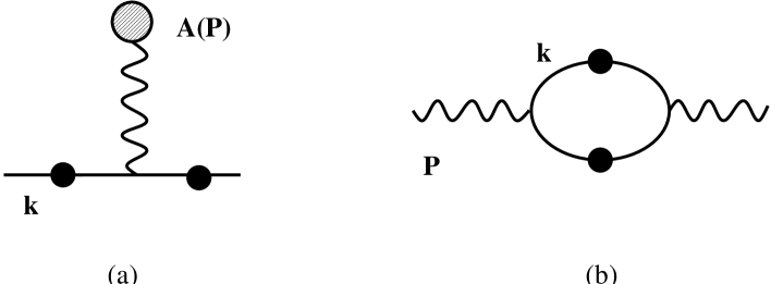
Figure 8: Diagrammatic representation of eq. (4.5): (a) the first-order fluctuation $\delta N^{(0)}(k,P)$, as induced by the mean field $A^{\mu}(P)$; (b) the corresponding contribution to the polarization tensor $\Pi^{\mu\nu}(P)$. The continuous line with a blob denotes the hard gluon propagator after the inclusion of the damping rate.

For more clarity, consider the response of the plasma to an arbitrarily weak electric mean field ${\bf E}_{a}$. Then, non-linear effects are negligible and the relevant response function is the polarization tensor: $j^{\mu}_{a}(P)\simeq\Pi^{\mu\nu}(P)A_{\nu}^{a}(P)$, where $P\sim g^{2}T$ is the (ultrasoft) momentum carried by the background field. In the mean field approximation, and to linear order in the electric field, the induced fluctuation reads (cf. eq. (3.55)):

$$\delta N(k,P)\,=\,{-g{\bf v\cdot E}(P)\over v\cdot P+i\eta}\,{{\rm d}N\over{\rm d}k}\,,$$ (4.4)

where the small imaginary part $i\eta$ with $\eta\to 0_{+}$ stands for retarded boundary conditions.

After adding the collision terms, we end up with an integro-differential equation for $\delta N$ (see, e.g., eqs. (3.8) or (4.1)), whose resolution is non-trivial already in the weak field limit. However, in order to see what are the relevant graphs, it is sufficient to consider the perturbative solution obtained by iterations. First, it is straightforward to resum the equilibrium damping rate $\Gamma$ (i.e., the collision term $C_{1}$): according to eqs. (4.1) and (4.2), this amounts to including the damping rate in eq. (4.4). This provides us with the 0th order iteration for $\delta N$:

$$\delta N^{(0)}(k,P)\,=\,{-g{\bf v\cdot E}(P)\over v\cdot P+2i\gamma}\,{{\rm d}N\over{\rm d}k}\,.$$ (4.5)

This can be given the diagrammatic representation in Fig. 8.a where the blob on the continuous line denotes the resummation of the damping rate in the hard gluon propagator, and the wavy line with a bubble attached to it represents a mean field insertion. In this approximation, the polarization tensor $\Pi^{\mu\nu}(P)$ is given be the one-loop diagram in Fig. 8.b.

With $\delta N^{(0)}$ as above, we can compute the first iteration for the collision terms $C_{2i}$, $i=1,\,2,\,3$. We shall not write down the corresponding formulae, but simply look for their interpretation in terms of Feynman graphs. The term $C_{21}$ in eq. (3.8) is associated with a fluctuation $\delta N(k^{\prime},X)$ in the hard, lower, propagator in Fig. 4; its first iteration is obtained by using the approximation (4.5) for this fluctuation, and has the diagrammatic representation in Fig. 9.a. To the same order, $C_{22}$ is represented in Fig. 9.b, while $C_{23}$ has a similar representation. With these approximations for the collision terms, one can compute the first iteration $\delta N^{(1)}(k,P)$, as well as its contribution to $\Pi^{\mu\nu}(P)$: the latter is shown in Figs. 10.a and 10.b. Clearly, Fig. 10.a is a vertex correction, which has to supplement the self-energy resummations in Fig. 8.b as required by gauge symmetry. Similarly, the diagram in Fig. 10.b is a different kind of vertex correction which involves two hard loops (and one soft one).

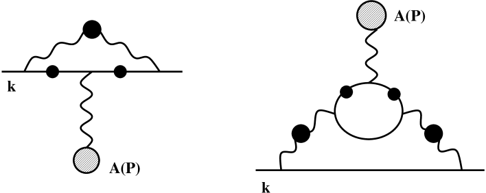
Figure 9: Diagrammatic representation of the collision terms $C_{21}$ (fig. (a)) and $C_{22}$ (fig. (b)), as computed with the first-order fluctuation $\delta N^{(0)}(k,P)$. The wavy line with a blob denotes the soft gluon propagator in the HTL approximation. The other notations are as in Fig. 8.

It should be clear by now what are the diagrams generated by further iterations: these are the ladder diagrams displayed in Fig. 11 where the continuous lines are hard transverse gluons dressed with the damping rate $\Gamma$, and the (internal) wavy lines are soft gluons which may be longitudinal or transverse and are dressed with the hard thermal loop. Indeed, the phase-space integrals giving $\Gamma$ and $C_{2i}$ are individually dominated by soft $q$ momenta, in the range $g^{2}T\mathrel{\hbox to0.0pt{\raise 2.20013pt\hbox{$<$}\hss}{\lower 2.20013pt\hbox{$\sim$}}}q\mathrel{\hbox to0.0pt{\raise 2.20013pt\hbox{$<$}\hss}{\lower 2.20013pt\hbox{$\sim$}}}gT$. Note also that the diagrams in Fig. 11 may involve an arbitrary number of loops. However, from the previous derivation of the Boltzmann equation, we know that, for an external momentum $P\sim g^{2}T$, they all contribute at the same order in $g$, namely, at the same order as the corresponding hard thermal loop [1, 2] (see also Ref. [47]).

Figure 10: Loop corrections to the polarization tensor in Fig. 8.b, as generated by the collision terms depicted in Fig. 9.

Except for the colour structure of the vertices, similar diagrams are resummed by the Abelian Boltzmann equation as well. There too, the damping rate $\Gamma$ of the charged particle is dominated by soft momenta transfer, and, in fact, it coincides with the corresponding rate for gluons up to a colour factor (compare eqs. (2.82) and (3.107)). Nevertheless, we have seen in Sec. 2.6 that the Abelian collision terms are not dominated by soft momenta exchange, but receive contributions from all the momenta between $gT$ and $T$. In order for this to be consistent with the diagrammatic picture in Fig. 11, there must be some cancellations among the Feynman graphs, in such a way that the globl contribution of soft ($q\mathrel{\hbox to0.0pt{\raise 2.20013pt\hbox{$<$}\hss}{\lower 2.20013pt\hbox{$\sim$}}}gT$) internal photons cancels out in their sum.

The relevant cancellations have been discussed in Sec. 2.6, and can be also read off the formulae in Sect. 3.8. The contributions of the soft exchanged momenta $q\mathrel{\hbox to0.0pt{\raise 2.20013pt\hbox{$<$}\hss}{\lower 2.20013pt\hbox{$\sim$}}}gT$ to the individual collision terms are listed in eqs. (3.107), (3.108) and (3.110). If there was not for the colour structure, the vertex correction in eq. (3.108) would exactly cancel the self-energy correction in eqs. (3.107). This is what happens in the Abelian case (cf. the discussion in Sec. 2.6) and explains, for instance, why there is no effect of the damping rate $\gamma\sim e^{2}T\ln(1/e)$ of the charged particle on the polarization tensor $\Pi_{\mu\nu}$ for soft photons. Diagramatically, this corresponds to a cancellation of the soft photon effects in between self-energy and vertex corrections in any of the bubbles depicted in Fig. 11, as it has been also verified via the direct analysis of the Feynman graphs, by Lebedev and Smilga [30] (see also Refs. [42, 48]).

Figure 11: A generic ladder diagram of the type resummed in the solution to the Boltzmann equation.

Similarly, in the absence of colour effects, there would be an exact cancellation between the soft contributions to $C_{22}$ and $C_{23}$ (cf. eq. (3.110)): if we refer to the diagram in Fig. 9b, this cancellation reflects the well known fact that there is no photon HTL with three (or more) external legs [1, 2].

In QCD, on the other hand, these cancellations are not complete, because of the non-trivial colour structure (cf. eqs. (3.109) and (3.110)). In fact, for $\delta N(k,X)\equiv\delta N_{a}T^{a}$, we have (refer to eq. (3.108)) $(T^{a}T^{b})_{cd}\delta N_{cd}=(N_{c}/2)\delta N_{ab}$, so that the vertex correction in eq. (3.108) only cancels half of the damping rate contribution in eq. (3.107). Furthermore, since $\delta N\equiv\delta N_{a}T^{a}$ is an antisymmetric colour matrix, the two terms $C_{22}$ and $C_{23}$ give identical contributions which add together (rather than subtract, as in QED) to give the final result in eq. (3.110). Accordingly, the polarization tensor $\Pi_{\mu\nu}(P)$ for soft ($P\sim g^{2}T$) gluons is sensitive to the hard gluon damping rate $\gamma\sim g^{2}T\ln(1/g)$, as discussed at the end of the previous section. (To our knowledge, this has been first observed by Bödecker [6].)

The previous discussion also shows that, for colourless fluctuations in the hot QCD plasma (as involved, for instance, in the calculation of the shear viscosity), the pattern of the cancellations is the same as in QED: the relevant collision terms are dominated by relatively large ($gT\mathrel{\hbox to0.0pt{\raise 2.20013pt\hbox{$<$}\hss}{\lower 2.20013pt\hbox{$\sim$}}}q\mathrel{\hbox to0.0pt{\raise 2.20013pt\hbox{$<$}\hss}{\lower 2.20013pt\hbox{$\sim$}}}T$) transferred momenta. Thus, the typical inverse relaxation time for such fluctuations is $\tau^{-1}\sim g^{4}T\ln(1/g)$, where the logarithm comes from $\log(T/m_{D})$, that is, from the screening effects at the scale $gT$ [9, 14, 15].

5 Conclusions

Starting from first principles, we have derived a Boltzmann equation which describes the long wavelength colour excitations of a high temperature Yang-Mills plasma. Our derivation relies on a gauge-covariant gradient expansion of the Kadanoff-Baym equations for the off-equilibrium dynamics of the plasma. This expansion can be also intrepreted as an expansion in powers of $g$, in the sense that the plasma inhomogeneities (the “soft” gradients $\partial_{X}$), the strength of the colour mean fields $A^{\mu}_{a}$ and the off-equilibrium deviations of the distribution functions are all contolled by powers of $g$. Specifically, our derivation applies to the case where $\partial_{X}\sim gA\sim g^{2}T$, so that the soft covariant derivatives $D_{X}=\partial_{X}+igA\sim g^{2}T$ are consistently preserved in the perturbative expansion. This, together with a judicious choice of the gauge fixing (the background field gauge) and a proper definition of gauge-covariant Wigner functions, has allowed us to maintain explicit gauge symmetry at all steps of our construction.

In this framework, the Boltzmann equation has emerged as the quantum transport equation at leading order in $g$. Note that our present, leading order, perturbative expansion encompasses several approximations which are generally seen as independent approximations when deriving transport equations: the gradient expansion (slowly varying disturbances), the weak field expansion (small perturbations), the quasiparticle approximation (well defined “quasiparticles”, with a long lifetime) and the (dressed) Born approximation (one-gluon exchange) for the collision term. Note also that, in spite of being obtained within a systematic perturbative expansion, the Boltzmann equation actually resums an infinite series of ladder diagrams and therefore generates a non-perturbative effective theory for the “ultrasoft” ($\partial_{X}\sim g^{2}T$) colour fields. For instance, the polarization tensor for these fields, as obtained by solving the Boltzmann equation, is equivalent to the sum of an infinite number of ladder diagrams of the perturbation theory.

Remarkably, the colour structure of the collision terms is precisely that predicted by Arnold, Son and Yaffe, on the basis of simple heuristic arguments [7] (this is also consistent with some previous results in Refs. [17, 10, 12]). Accordingly, the effective theory generated by our Boltzmann equation is precisely that obtained by Bödecker using a different method [6] (see Ref. [7] for a discussion of the relation between the Boltzmann equation and Bödecker’s theory).

It is important to emphasize the accuracy limits of the Boltzmann equation presented here. The collision term in eq. (1.2) is only known to logarithmic accuracy, which means that both its functional form and the overall coefficient $\gamma$ which fixes the time scale for colour relaxation are known only up to corrections of relative order $1/\ln(1/g)$. For instance, $\gamma=\alpha N_{c}T\Bigl{(}\ln(1/g)+{\rm O}(1)\Bigr{)}$ where the constant terms under the logarithm is not accurately given by the present formalism. There are two main sources for such a limitation: (i) The gradient expansion in the presence of long range interactions: the one-gluon exchange interaction has a typical range $\sim 1/q$ with $g^{2}T\mathrel{\hbox to0.0pt{\raise 2.20013pt\hbox{$<$}\hss}{\lower 2.20013pt\hbox{$\sim$}}}q\mathrel{\hbox to0.0pt{\raise 2.20013pt\hbox{$<$}\hss}{\lower 2.20013pt\hbox{$\sim$}}}gT$ which is marginally the same as the inhomogeneity scale in the problem, $\lambda\sim 1/g^{2}T$. Since the collision terms are only logarithmically sensitive to the low momenta $q\sim g^{2}T$, it follows that the gradient expansion for the collision kernel (i.e., for the exchanged gluon propagator in eq. (3.90)) is only correct to logarithmic accuracy. As discussed after eq. (3.92), this limitation can be avoided, at least in principle, by relaxing the gradient expansion so as to allow for a collision kernel which is non-local in $X$. (ii) Still related to the long-ranged collision kernel: the behaviour of the gluon propagator at very soft momenta $q\sim g^{2}T$ is not correctly described by the HTL approximation, since it is sensitive to the non-perturbative physics.

Of course, the Boltzmann equation constructed in this paper can also be used to study colourless fluctuations, as involved, e.g., in the calculation of the shear viscosity [9, 14, 34]. The relevant collision terms are displayed in eqs. (3.99), (3.101) and (3.8), where the off-equilibrium fluctuations have now a trivial colour structure (e.g., $\delta\acute{G}_{\bar{d}d}(p,X)\equiv\delta_{\bar{d}d}\delta\acute{G}(p,X)$, etc.). This yields the standard Boltzmann equation (in its linearized version), as already used in calculations of the shear viscosity for the quark gluon plasma [9, 14].

References

- [1] J.-P. Blaizot, E. Iancu and J.-Y. Ollitrault, in Quark-Gluon Plasma II, Edited by R.C. Hwa (World Scientific, Singapore, 1996).
- [2] M. Le Bellac, Thermal Field Theory, (Cambridge University Press, Cambridge, 1996).
- [3] J.-P. Blaizot and E. Iancu, “The weakly coupled quark-gluon plasma: collective dynamics and hard thermal loops”, to appear in Physics Reports.
- [4] J.P. Blaizot and E. Iancu, Phys. Rev. Lett. 70 (1993) 3376; ibid. Nucl. Phys. B417 (1994) 608.
- [5] J.P. Blaizot and E. Iancu, Nucl. Phys. B421 (1994) 565; ibid. B434 (1995) 662.
- [6] D. Bödeker, Phys. Lett. B426 (1998) 351.
- [7] P. Arnold, D. Son and L. Yaffe, “Hot B violation, color conductivity, and log(1/alpha) effects”, hep-ph/9810216; ibid. “Longitudinal subtleties in diffusive Langevin equations for non-Abelian plasmas”, hep-ph/9901304.
- [8] U. Heinz, Phys. Rev. Lett. 51 (1983) 351; ibid. Ann. Phys. 161 (1985) 48.
- [9] G. Baym, H. Monien, C.J. Pethick, and D.G. Ravenhall, Phys. Rev. Lett. 64 (1990) 1867.
- [10] A. V. Selikhov and M. Gyulassy, Phys. Lett. B316 (1993) 373; Phys. Rev. C49 (1994) 1726.
- [11] H. Heiselberg and C.J. Pethick, Phys. Rev. D47 (1993) R769.
- [12] H. Heiselberg, Phys. Rev. Lett. 72 (1994) 3013.
- [13] P.F. Kelly, Q. Liu, C. Lucchesi and C. Manuel, Phys. Rev. Lett. 72 (1994) 3461; ibid. Phys. Rev. D50 (1994) 4209.
- [14] H. Heiselberg, Phys. Rev. D49 (1994) 4739
- [15] G. Baym and H. Heiselberg, Phys. Rev. D56 (1997) 5254.
- [16] D.F. Litim and C. Manuel, “Mean field dynamics in non-Abelian plasmas from classical transport theory”, hep-ph/9902430.
- [17] A.V. Selikhov, Phys. Lett. B268 (1991) 263; ibid. B285 (1992) 398(E).
- [18] H.-Th. Elze, M.Gyulassy and D. Vasak, Nucl. Phys. B276 (1986) 706; Phys. Lett. B177 (1986) 402.
- [19] D. Vasak, M. Gyulassy and H.-Th. Elze, Ann. Phys. 173 (1987) 462.
- [20] H.-Th. Elze, Z.Phys. C38 (1988) 211; ibid. C47 (1990) 647.
- [21] H.-Th. Elze and U. Heinz, Phys. Repts. 183 (1989) 81.
- [22] S. Mrówczyński, in Quark-Gluon Plasma, edited by R.C. Hwa, (World Scientific, Singapore, 1990).
- [23] D. Bödeker, L. McLerran and A. Smilga, Phys. Rev. D52, 4675 (1995).
- [24] P. Arnold, D. Son and L. Yaffe, Phys. Rev. D55 (1997) 6264.
- [25] C. Hu and B. Müller, Phys. Lett. B409 (1997) 377; G.D. Moore, C. Hu and B. Müller, Phys. Rev. D58 (1998) 045001.
- [26] E. Iancu, Phys. Lett. B435 (1998) 152; ibid. “Classical theory for nonperturbative dynamics in hot QCD”, hep-ph/9809535.
- [27] G.D. Moore, “The sphaleron rate: Bodeker’s leading log”, hep-ph/9810313.
- [28] R.D. Pisarski, Phys. Rev. Lett. 63 (1989) 1129; E. Braaten and R.D. Pisarski, Nucl. Phys. B337 (1990) 569; ibid. Phys. Rev. D42 (1990) 2156.
- [29] J. Frenkel and J.C. Taylor, Nucl. Phys. B334 (1990) 199; J.C. Taylor and S.M.H. Wong, Nucl. Phys. B346 (1990) 115; R. Efraty and V.P. Nair, Phys. Rev. Lett. 68 (1992) 2891; R. Jackiw and V.P. Nair, Phys. Rev. D48 (1993) 4991.
- [30] V.V Lebedev and A.V. Smilga, Ann. Phys. 202 (1990) 229; Physica A181 (1992) 187.
- [31] R.D. Pisarski, Phys. Rev. D47 (1993) 5589.
- [32] J.P. Blaizot and E. Iancu, Phys. Rev. Lett. 76 (1996) 3080; ibid. Phys. Rev. D55 (1997) 973; ibid. D56 (1997) 7877.
- [33] S. Jeon, Phys. Rev. D47 (1993) 4568; ibid. D52 (1995) 3591.
- [34] S. Jeon and L. Yaffe, Phys. Rev. D53 (1996) 5799.
- [35] L.Kadanoff and G.Baym, Quantum Statistical Mechanics, (Benjamin, New York,1962).
- [36] J. Schwinger, J. Math. Phys. 2 (1961) 407.
- [37] P.M. Bakshi and K.T. Mahanthappa, J. Math. Phys. 4 (1963) 1; ibid. 4 (1963) 12.
- [38] L.V. Keldysh, Sov. Phys. JETP 20 (1964) 1018.
- [39] E.M. Lifshitz and L.P. Pitaevskii, Physical Kinetics (Pergamon Press, Oxford, 1981).
- [40] P. Danielewicz, Ann. Phys. 152 (1984) 239.
- [41] S. Mrówczyński and U. Heinz, Ann. Phys. 229 (1994) 1.
- [42] U. Kraemmer, A. Rebhan and H. Schulz, Ann. Phys. 238 (1995) 286.
- [43] G. Baym and C.J. Pethick, Landau Fermi-liquid theory: concepts and applications, (J. Wiley, N.Y., 1991).
- [44] D. Boyanovsky and H.J. de Vega, “Anomalous kinetics of hard charged particles: dynamical renormalization group resummation”, hep-ph/9812504.
- [45] B.S. De Witt, Phys. Rev. 162 (1967) 1195, 1239; ibid. Phys. Repts. 19C (1975) 295.
- [46] L. F. Abbott, Nucl. Phys. B185 (1981) 189.
- [47] J.P. Blaizot and E. Iancu, in preparation.
- [48] E. Petitgirard, Phys. Rev. D59 (1999) 045004.