Quarks and Leptons Beyond the Third Generation.

Abstract

The possibility of additional quarks and leptons beyond the three generations already established is discussed. The make-up of this Report is (I) Introduction: the motivations for believing that the present litany of elementary fermions is not complete; (II) Quantum Numbers: possible assignments for additional fermions; (III) Masses and Mixing Angles: mass limits from precision electroweak data, vacuum stability and perturbative gauge unification; empirical constraints on mixing angles; (IV) Lifetimes and Decay Modes: their dependence on the mass spectrum and mixing angles of the additional quarks and leptons; the possibility of exceptionally long lifetimes; (V) Dynamical Symmetry Breaking: the significance of the top quark and other heavy fermions for alternatives to the elementary Higgs Boson; (VI) CP Violation: extensions to more generations and how strong CP may be solved by additional quarks; (VII) Experimental Searches: present status and future prospects; (VIII) Conclusions.

I Introduction.

The elementary spin-half fermions as we now know them are the quarks and leptons. The principal constituents of normal atoms and normal matter are the electron, as well as the up and down quarks which comprise the valence quarks of the protons and neutrons in the atomic nucleus. In addition, there is the electron neutrino which was first postulated by Pauli[1] in 1931 to explain conservation of energy and angular momentum in nuclear $\beta$-decay, and which was eventually discovered in 1956 by Reines and Cowan[2].

These quarks and leptons - the up and down quarks, the electron and its neutrino - comprise what is now called the first generation. The first intimation that Nature is more complex came with the discovery of the muon in 1937[3, 4]. The muon appears identical to the electron except for its mass which is $\sim 200$ times heavier. The muon appeared so surprising that there was a famous comment by I.I. Rabi[5]: ”Who ordered that?”

The fact that the muon neutrino differs from the electron neutrino was established in 1962[6]. The strange quark had already been discovered implicitly through the discovery of strange particles beginning in 1944[7, 8, 9]. Completion of the second family with the charmed quark, predicted in 1970[10], was accomplished in 1974[11, 12, 13, 14]. At first only hidden charm was accessible but two years later explicit charm was detected[15].

By this time, a renormalizable gauge theory was available [16, 17, 18, 19, 20] based on the first two generations and incorporating the Cabibbo mixing[21] between the two generations.

The situation became even more challenging to theorists when experimental discovery of the third generation of quarks and leptons began with the tau lepton, discovered in 1975[22] in $e^{+}e^{-}$ scattering at SLAC. Next was the bottom quark in 1977 [23, 24]. The top quark, at $\sim 175\$GeV much heavier than originally expected, was finally discovered in 1995[25, 26]. Together with the $\tau$ neutrino which presumably participates (its distinct identity - while not questioned - is not fully demonstrated) in tau decay, this completed the third generation.

Since the present review is dedicated to the premise of further quarks and leptons beyond the third generation, it is worthwhile to recall to what extent and how the third generation was anticipated from the existence of the first two generations, why it is regarded as the end of the litany of quarks and leptons and what loopholes there are in the latter arguments.

One early theoretical anticipation of a third generation was the paper of Kobayashi and Maskawa[27] who pointed out, at a time (1973) when only three flavors u, d, s of quark were established, that the existence of six flavors in three generations would allow the standard model naturally to accommodate CP violation.

Study of the formation of the light elements (Hydrogen, Deuterium, Helium, and Lithium) in the early universe was started earlier in the 1960’s [28, 29]. In the 1970’s tighter constraints were found based on the steadily-improving estimates of the primordial abundances of these light isotopes. Since the expansion rate of the universe in this era of Big-Bang Nucleosynthesis, and hence the abundances, depends sensitively on the number of light neutrinos it was then possible to limit the acceptable number. The group of Schramm et al.[30, 31, 32] found in this way that the number of generations should not be greater than four[30], or in some analyses not greater than three (see e.g. footnote 4 on page 242 of[31]); it is surely remarkable that such a strong constraint was found from early universe considerations already in 1979, a decade before the situation was clarified using colliders.

A current plot of the primordial ${}^{4}He$ abundance (whose exact value is still controversial in 1998) versus neutrino number $n(\nu)$ for $n(\nu)=3.0,3.2,3.4$ is given in Figure $1$. The main point is that the neutrino number from cosmology is by now tied very closely to the high-energy experimental value in what is the strongest known link between particle theory and cosmology.

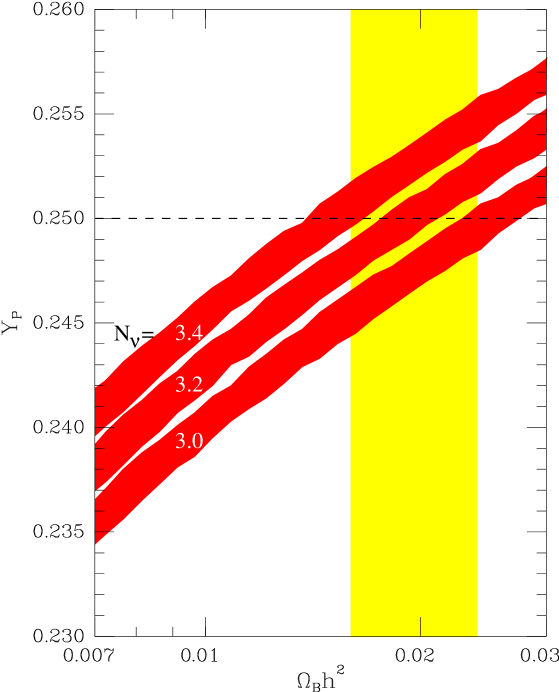
FIG. 1.: Helium-4 production for $N_{\nu}=3.0,3.2,3.4$. The vertical band indicates the baryon density consistent with $(D/H)_{P}=(2.7\pm 0.6)\times 10^{-5}$ and the horizontal line indicates a primeval Helium-4 abundance of $25\%$. The widths of the curves indicate the two-sigma theoretical uncertainty. Figure from Ref. [33].

In 1989, there came an experimental epiphany concerning the number of generations, or more precisely, the number of light neutrinos. This arose from the measurement of the Z width at SLAC[34, 35] and especially at CERN [36, 37, 38, 39]. The answer from this source is indisputably equal to three. The argument is simple: One can measure the total width of the $Z$ to high accuracy, and then subtract the visible width to get the invisible width. Identifying the invisible width with neutrino decays leads to[40]:

$$n(\nu)=3.00\pm 0.025$$ (1)

This provides compelling proof that there are only three conventional neutrinos with mass below $M_{Z}/2\simeq 45$ GeV. And, by extrapolation, it leads to the idea that there are only three quark-lepton families. Since this ties in nicely with the KM mechanism of CP violation and with the Big-Bang-Nucleosynthesis, the overall picture looks very attractive.

However, this finality was not universally accepted[41, 42]. There are other reasons for entertaining the possibility of further quarks and leptons:

• In many grand-unified theories (GUTs), there naturally occur additional fermions. Although the minimal $SU(5)$ GUT can contain only the basic three families, extension to any higher GUT such as $SO(10)$ or $E(6)$ inevitably adds new fermions. In $SO(10)$ this may be only right-handed neutrinos (leptons) but in $E(6)$ there are also non-chiral color triplets(quarks) and color singlet(leptons). Although there is no direct evidence for GUTs they are attractive theoretically and suggestive of how the standard nodel is extended.

• Models of CP violation which solve the strong CP problem without axions generically require additional quarks.

• For some models of dynamical symmetry breaking[43, 44, 45, 46] the top quark mass, although higher than originally expected, is still not quite high enough to play its role in electroweak symmetry breaking. This might be interpreted as evidence for even heavier quarks.

• It has been shown that a non-supersymmetric model with four generations can have successful unification of the gauge couplings at the unification scale.

• In recently-popular models of gauge-mediated supersymmetry breaking, additional vectorlike quarks and leptons arise automatically. In addition, in models in which higher dimensions arise at the TeV scale[47], it has been shown[48] that if some standard model fields live in the higher dimensional space, low-scale gauge unification can be obtained–the Kaluza-Klein excitations of these fields, which could be rather light, must be vectorlike.

None of these reasons is fully compelling but each is suggestive that one should keep alive the study of this issue. Our hope is that this review will play a role in encouraging further thought about this open question.

The present review contains the following subsections: Section II is on the possible quantum numbers of additional quarks and leptons; Section III discusses their masses and mixing angles; Section IV deals with lifetimes and decay modes; Dynamical symmetry breaking is in Section V; CP violation is treated in Section VI, and finally in Section VII there is a treatment of the experimental situation and in Section VIII are the conclusions.

II Quantum Numbers.

When we add fermions to the standard model, there are choices in the possible quantum numbers.

Under the color $SU(3)_{C}$ group we refer to color triplets as quarks, color antitriplets as antiquarks. Color singlets which do not experience the strong interaction are generically referred to as leptons. Higher representations of color such as $6$, $\bar{6}$, $8$,… may be called quixes, antiquixes, queights, and so on. Such exotic color states are necessary in some models to cancel chiral anomalies. For example, in chiral color[49, 50] one version (called Mark II in[49]) involves three conventional fermion generations, an extra $Q=2/3$ quark, and an $SU(3)$ sextet fermion or quix. The extended gauge group of chiral color is $SU(3)_{L}\times SU(3)_{R}\times SU(2)_{L}\times U(1)_{Y}$ and we may list the fermions by their $(SU(3)_{L},SU(3)_{R},Q)$ quantum numbers. There are three colored weak doublets

$$3[(3,1,\frac{2}{3})+(3,1,-\frac{1}{3})],$$ (2)

eight colored weak doublets

$$4(1,\bar{3},-\frac{2}{3})+3(1,\bar{3},+\frac{1}{3})+(3,1,\frac{2}{3}),$$ (3)

a weak singlet quix

$$(\bar{6},1,-\frac{1}{3})+(1,6,\frac{1}{3}),$$ (4)

and three charged leptons and their neutrinos. The quix plays an essential role in anomaly cancellation. But in this review we restrict our attention only to quarks and leptons because while more exotic color states are a logical possibility it is one which is difficult to categorize systematically.

Quarks and leptons may be either chiral or non-chiral. The latter are sometimes alternatively called vector-like. Let us therefore define the meaning of these adjectives.

Chiral fermions are, for present purposes, spin-$\frac{1}{2}$ paricles where the left and right components transform differently under the electroweak gauge group $SU(2)_{L}\times U(1)$. All the fermions of the standard model are chiral. This means that they are strictly massless before the electroweak symmetry is broken.

The simplest generalization of the standard model is surely to add a fourth sequential family. Of course, a fourth light neutrino is an immediate phenomenological problem with the invisible $Z$ width, but the addition of a right-handed neutrino can resolve this.

More generally we may add a chiral doublet quark or lepton where the left-handed components transform as a doublet of $SU(2)_{L}$ and the right-handed components as singlets. A chiral doublet of quarks is:

$$\left(\begin{array}[]{c}U\\ D\end{array}\right)_{L};\hskip 14.45377ptU_{R};\hskip 14.45377ptD_{R}$$ (5)

while a chiral doublet of leptons is

$$\left(\begin{array}[]{c}N\\ E\end{array}\right)_{L};\hskip 14.45377ptN_{R};\hskip 14.45377ptE_{R}$$ (6)

Equally possible are chiral singlets such as

$$U_{L}$$ (7)

or

$$D_{L}$$ (8)

for quarks, or for leptons

$$N_{L}$$ (9)

or

$$E_{L}$$ (10)

Of course, with chiral doublets or singlets, there is a constant danger of chiral anomalies. In the standard model, there is a spectacular cancellation in each generation between the anomalies of the chiral doublets of quarks and leptons. In other models one sometimes adds mirror chiral doublets to cancel anomalies. For example, a mirror chiral doublet of quarks is

$$U_{L};\hskip 14.45377ptD_{L};\hskip 14.45377pt\left(\begin{array}[]{c}U\\ D\end{array}\right)_{R}$$ (11)

There can also be non-chiral (also known as vector-like) fermions, where the right and left components transform similarly under the electroweak $SU(2)\times U(1)$ group. For example a vector-like quark doublet is

$$\left(\begin{array}[]{c}U\\ D\end{array}\right)_{L};\hskip 14.45377pt\left(\begin{array}[]{c}U\\ D\end{array}\right)_{R}$$ (12)

A vector-like doublet is not to be confused with the doublets occurring in the left-right model[51, 52, 53] where the gauge group is extended to $SU(2)_{L}\times SU(2)_{R}\times U(1)_{B-L}$. The U and D quarks transform there chirally as in (5) above under $SU(2)_{L}$, but the right-handed singlets $U_{R}$ and $D_{R}$ of $SU(2)_{L}$ are then assumed to transform as a doublet under the additional gauge group $SU(2)_{R}$.

General patterns for adding anomaly-free charge-vectorial chiral sets of fermions which acquire mass by coupling to the Higgs doublet of the standard model have been studied in [54] and further developed in [55, 56]. An extensive analysis of the possible quantum numbers for additional fermions can be found in Ref. [57]. They looked at the general structure of exotic generations given the gauge and Higgs structure of the standard model. A similar analysis for left-right symmetric models was carried out in Ref. [58].

In grand unified theories (GUTs) all types of additional fermions are possible. For example, in $SU(5)$ there may be no additional fermions. But in $SO(10)$ there must be at least an additional chiral right-handed neutrino in each family. In $E(6)$ each 27 of fermions contains not only two extra neutrino-like states but also a ${\bf 5+\bar{5}}$ of $SU(5)$ which contains a non-chiral singet of quarks and a non-chiral doublet of leptons.

In superstring models, and M-theory models, the additional fermions are even less constrained. For example $E(6)$ and its content has been a familiar superstring possibility since the beginning[4], and any gauge group contained in at least $O(44)$ is possible. Families and anti (mirror) families often occur in superstrings.

Some extensions of the standard model require extra chiral fermions to cancel anomalies e.g.

• As already mentioned, chiral color[49], anomaly cancellation dictates addition of quixes.

• In some GUTs, e.g. $SU(15)$ anomaly cancellation requires[60] inclusion of mirror fermions.

More interesting are the types of additional quarks and leptons appearing in extensions of the standard model motivated by attempting to explain shortcomings of the model itself.

Examples are:

• Attempts to solve the strong CP problem without an axion[61, 62] can introduce a non-chiral doublet of quarks, or non-chiral singlets (but not both),

• In trying to explain the three families through anomaly cancellation, the 331-model[63, 64] extends the individual families of the standard model by adding non-chiral singlets of quarks. The charges of the additional quarks differ between the families. In a sense, this is not “Quarks and Leptons beyond the Third Generation” since the quarks are being added to the discovered generations. Nevertheless, our framework is sufficiently general to accommodate this possibility - as additional non-chiral singlets of quarks.

• In the non-supersymmetric standard model, gauge unification of the couplings fail–the three couplings do not meet at a point. It has been noted[65] that extending the model to allow a fourth generation introduces enough flexibility that a successful unification of couplings can occur.

• A potential problem of the minimal supersymmetric standard model is that the scalar quark masses must be very nearly degenerate to avoid large tree-level flavor-changing neutral currents. This degeneracy is very unnatural, using the conventional mechanism of gravitationally mediated supersymmetry breaking (where the supersymmetry breaking part of the Lagrangian is transmitted to the known sector via gravitational interactions). However, in gauge-mediated supersymmetry breaking, the supersymmetry breaking is transmitted to the known sector via the gauge interactions of “messenger” fields. Since the gauge interactions are flavor-blind, the degeneracy of squark masses is natural. The messenger fields are, in the simplest case, composed of a $5+\bar{5}$ of $SU(5)$ (or of several such fields), which constitute a vectorlike $Q=-1/3$ quark and a vectorlike lepton.

• There has been recent excitement about the possibility that additional spacetime dimensions could be compactified at (or even well below) the TeV scale[47]. In such models, the Kaluza-Klein excitations must be vectorlike (to avoid having, for example, too many light neutrinos).

In this Report, we will primarily concentrate on chiral quarks and leptons, or vectorlike quarks and leptons, since they appear in the majority of models. However, when appropriate, we will note how our various constraints and bounds will apply to mirror quarks.

III Masses and Mixing Angles.

One of the most unsatisfactory features of the standard model is the apparent arbitrariness of the masses and mixing angles of the known fermions. Although masses and mixing angles can be accommodated in the standard model (with addition of right handed neutrino fields, if necessary), there is no understanding of their values. An entire industry of model-building has developed in an attempt to provide some theoretical guidance, ranging from flavor symmetries to relationships from grand unification, but no model seems particularly compelling.

In the case of additional fermions, the masses and mixing angles also are arbitrary. Nonetheless, some general features can be found. Phenomenological bounds can be obtained from high precision electroweak studies, theoretical bounds can be obtained from requiring the stability of the standard model vacuum and from requiring that perturbation theory be valid (up to some scale). In this Section, these bounds are explored in some detail. We will start with a discussion of the phenomenological constraints from precision electroweak studies. Then we will consider bounds from vacuum stability and perturbation theory. In the vast majority of analyses of these bounds, the authors focused on bounds to the top quark mass, since its mass was unknown until relatively recently, thus we will first look at constraints on the top quark mass, and then generalize the results to find bounds on masses of additional quarks and leptons. Finally, we will discuss plausible models for the mixing angles.

A Precision Electroweak Constraints

1 Chiral Fermions

In the past decade, high precision electroweak measurements have led to remarkable constraints on potential physics beyond the standard model. The most important of these is the $\rho$ parameter. As originally pointed out by Veltman[66, 67], the tree level mass relation

$$\rho\equiv{M^{2}_{W}\over M_{Z}^{2}\cos^{2}\theta_{W}}=1$$ (13)

is very sensitive to non-standard model physics (ruling out, for example, significant vacuum expectation values for Higgs triplets). Since the relation is good to better than $1\%$, it is assumed that deviations from the relation are due to electroweak radiative corrections, which are sensitive to new particles in loops.

An extensive, detailed analysis of electroweak radiative corrections can be found (with a long list of references) in the work of Peskin and Takeuchi[68, 69]. They define the S and T parameters as

$$\alpha S \equiv 4e^{2}[\Pi^{\prime}_{33}(0)-\Pi^{\prime}_{3Q}(0)]$$ (14)

$$\alpha T \equiv{e^{2}\over\sin^{2}\theta_{W}M^{2}_{W}}[\Pi_{11}(0)-\Pi_{33}(0)]$$ (15)

where $\alpha$ is the fine-structure constant, $\Pi_{XY}(q^{2})$ is the vacuum-polarization amplitude with $(XY)=(11),(22),(33),(3Q),(QQ)$, and $\Pi^{\prime}={\Pi(q^{2})-\Pi(0)\over q^{2}}$. Roughly, $T$ is a measure of the deviation of the $\rho$ parameter from unity, coming from isospin violating contributions. $S$ is an isospin symmetric quantity which measures the momentum dependence of the vacuum polarization; it is roughly the “size” of the new physics sector

As an example, Peskin and Takeuchi consider the case of a chiral lepton doublet, $E$ and $N$. In the limit $M_{N},M_{E}>>M_{Z}$, they show that if the mass splitting is small, then the contribution for $S$ is just ${1\over 6\pi}$, and the contribution for $T$ is ${|\Delta M^{2}|\over 12\pi\sin^{2}\theta_{W}M^{2}_{W}}$. For a chiral quark doublet, these contributions are tripled. As stated above, one can see that $T$ is a measure of the isospin splitting, while $S$ is a measure of the size of the new sector. Thus, for a complete degenerate fourth generation, the contribution to $S$ is

$$S={2\over 3\pi}\sim 0.21$$ (16)

while the contribution to $T$ is

$$T={|\Delta M_{L}^{2}|\over 12\pi\sin^{2}\theta_{W}M^{2}_{W}}+{|\Delta M_{Q}^{2}|\over 4\pi\sin^{2}\theta_{W}M^{2}_{W}}$$ (17)

It is important to note that these results were obtained under the assumption that the extra fermion masses were much greater than that of the $Z$, and that the mass splitting was small. Peskin and Takeuchi give more exact expressions.

What are the experimental bounds? The values can be determined from the data on Z-pole asymmetries, $M_{Z}$, $M_{W}$, $R_{l}$, $m_{top}$, $R_{b}$ and Z-decay widths. The contribution from new physics, $S_{new}=S-S_{SM}$ and $T_{new}=T-T_{SM}$, can be determined[40, 71, 72]. The value of this contribution depends on the Higgs and top quark masses (which affect $S_{SM}$, for example). For a top mass of $175$ GeV and a Higgs mass between $M_{Z}$ and $1$ TeV, Erler and Langacker[72] find

$$S_{new} =-0.20^{+0.40}_{-0.33}\ (3\sigma)$$ (18)

One can immediately see a apparent conflict between Eqs. 16 and 18. Independent of the mass, a fourth generation chiral multiplet is roughly $3$ standard deviations off. This led Erler and Langacker to claim that a fourth sequential family is excluded at the $99.8\%$ confidence level.

However, there are several reasons why we believe it is premature to exclude a fourth sequential family. First, of course, is the fact that many $3\sigma$ effects in recent years have disappeared. Second, the results for $S$ are based on virtual heavy fermion loops. Any additional new physics will likely make a similar contribution. For example, Erler and Langacker show that the allowed range for $S$ in minimal SUSY is $-0.17^{+0.17}_{-0.12}$, where the error bars are $1\sigma$, and this is only in conflict by 2.2 standard deviations. Third, it has been noted[73] that Majorana neutrino masses (which may be needed to give neutrino masses in the right range) lower $S$, as do models which involve mixing of two scalar doublets[74], and this could reduce the discrepancy further. Finally, the result above assumed a degenerate family. If one uses the exact expressions, takes $M_{H}=180$ GeV, $M_{D}=M_{U}=150$ GeV, $M_{N}=100$ GeV and $M_{E}=200$ GeV, for example, one finds the contribution to $S$ to be approximately $0.11$, rather than $0.21$. This also would lower the discrepancy to slightly more than $2\sigma$.

For $S\sim 0.2$, the $2\sigma$ upper bound on $T$ is approximately $0.2$, leading to bounds on the mass splitting from Eq. 16. For quarks, the splitting must be less[72] than $54(M_{W}/M_{D})$ GeV and for leptons must be less than $162(M_{W}/M_{E})$ GeV, at the $2\sigma$ level. Note that for quark masses above $200$ GeV, the splitting must be less than 10 percent.

Of course, the extra fermions must not contribute significantly to the width of the $Z$, and their masses are thus bounded from below by $M_{Z}/2$. Other experimental bounds will be discussed in Section VII.

2 Non-chiral Doublets

Vector-like fermions do not contribute in leading order to $S$ and $T$, and thus the values of these parameters do not constrain their masses. However, since vector-like doublets do not couple to the Higgs boson, the mass terms involving the $E$ and the $N$ cannot violate isospin invariance, and thus the masses must be degenerate at tree-level, as must the masses of the $U$ and $D$. Even if one adds a singlet Higgs field, the degeneracy will remain. Only a Higgs triplet can split this degeneracy, but Higgs triplet vacuum expectation values are severely constrained by the $\rho$ parameter. We conclude (in the absence of sizeable mixing with lighter generations) that the masses of states in a vector-like doublet are degenerate at tree level. The masses will be split by a few hundred MeV due to electroweak radiative corrections–this calculation will be done in the next Section.

3 Other Fermions

Non-chiral singlets will have arbitrary mass terms and arbitrary couplings to any Higgs singlets. No constraints can be placed on their masses.

B Vacuum Stability Bounds

Upper bounds on fermion masses can be obtained from the requirement that fermionic corrections to the effective potential not destabilize the standard model vacuum. We will first discuss the effective potential, and its renormalization group improvement. Then, the bounds from the requirement of vacuum stability will be discussed, first for the top quark mass, and then for additional quarks and leptons.

1 The Effective Potential

An extensive review of the effective potential and bounds from vacuum stability appeared in 1989[75]. Since then, the potential has been improved, including a proper renormalization-group improvement of scalar loops, and the bounds have been refined to much higher precision. In addition, the discovery of the top quark has narrowed the region of parameter space that must be considered. In this section, we discuss the effective potential and its renormalization-group improvement.

It is easy to see how bounds on fermion masses can arise. The one-loop effective potential, as originally written down by Coleman and Weinberg[76] can be written, in the direction of the physical $\phi$ field, as

$$V(\phi)=V_{0}+V_{1}$$ (19)

where

$$V_{0}=-{1\over 2}\mu^{2}\phi_{c}^{2}+{1\over 4}\lambda\phi_{c}^{4}$$ (20)

and

$$V_{1}={1\over 64\pi^{2}}\sum_{i}(-1)^{F}\eta_{i}{\cal M}^{4}(\phi_{c})\ln{{\cal M}^{2}(\phi_{c})\over M^{2}}$$ (21)

where the sum is over all particles in the model, F is the fermion number, $\eta_{i}$ is the number of degrees of freedom of the field i, and ${\cal M}^{2}(\phi_{c})$ is the mass that the field has in the vacuum in which the scalar field has a value $\phi_{c}$. In the expression for $V_{1}$, we have ignored terms which can be absorbed into $V_{0}$–these will be fixed by the renormalization procedure. In the standard model, we have for the W-boson, ${\cal M}^{2}(\phi_{c})={1\over 4}g^{2}\phi_{c}^{2}$, for the Z-boson, ${\cal M}^{2}(\phi_{c})={1\over 4}(g^{2}+g^{\prime 2})\phi_{c}^{2}$, for the Higgs boson, ${\cal M}^{2}(\phi_{c})=-\mu^{2}+3\lambda\phi_{c}^{2}$, for the Goldstone bosons, ${\cal M}^{2}(\phi_{c})=-\mu^{2}+\lambda\phi_{c}^{2}$ and for the top quark ${\cal M}^{2}(\phi_{c})={1\over 2}h^{2}\phi_{c}^{2}$. For a very large values of $\phi$, quadratic terms are negligible and the potential becomes

$$V={1\over 4}\lambda\phi^{4}+B\phi^{2}\ln(\phi^{2}/M^{2})$$ (22)

where

$$B={3\over 64\pi^{2}}[4\lambda^{2}+{1\over 16}(3g^{4}+2g^{2}g^{\prime 2}+g^{\prime 4})-h^{4}]$$ (23)

One can see that if the top quark is very heavy, then $h$ is large and thus $B$ is negative. In this case, the potential is unbounded from below at large values of $\phi$. This is the origin of the instability of the vacuum caused by a heavy quark.

Although this form of the effective potential is well known, it is NOT useful in determining vacuum stability bounds. The reason is as follows. Suppose one denotes the largest of the couplings in a theory by $\alpha$, in the standard model,for example, $\alpha=[\max(\lambda,g^{2},h^{2})]/(4\pi)$. The loop expansion is an expansion in powers of $\alpha$, but is also an expansion in powers of logarithms of $\phi_{c}^{2}/M^{2}$, since each momentum integration can contain a single logarithmic divergence, which turns into a $\ln(\phi^{2}_{c}/M^{2})$ upon renormalization. Thus the $n$-loop potential will have terms of order

$$\alpha^{n+1}[\ln(\phi^{2}/M^{2})]^{n}$$ (24)

In order for the loop expansion to be reliable, the expansion parameter must be smaller than one. $M$ can be chosen to make the logarithm small for any specific value of the field, but if one is interested in the potential over a range from $\phi_{1}$ to $\phi_{2}$, then it is necessary for $\alpha\ln(\phi_{1}/\phi_{2})$ to be smaller than one. In examining vacuum stability, one must look at the potential at very large scales, as well as the electroweak scale, and the logarithm is generally quite large. Thus, any results obtained from the loop expansion are unreliable; in fact, the bound on the top quark mass can be off by more than a factor of two.

A better expansion, which does not have large logarithms, comes from solving the renormalization group equation (RGE) for the effective potential. This equation is nothing other than the statement that the potential cannot be affected by a change in the arbitrary parameter, $M$, i.e. $dV/dM=0$. Using the chain rule, this is

$$[M{\partial\over\partial M}+\beta(g_{i}){\partial\over\partial g_{i}}-\gamma\phi{\partial\over\partial\phi}]V=0$$ (25)

where $\beta=Mdg_{i}/dM$ and there is a beta function for every coupling and mass term in the theory. The $\gamma$ function is the anomalous dimension.

It is important to note that the renormalization group equation is exact and no approximations have been made. If one knew the beta functions and anomalous dimensions exactly, one could solve the RGE exactly and determine the full potential at all scales. Although we do not know the exact beta functions and anomalous dimensions, we do have expressions for them as expansions in couplings. Thus, by only assuming that the couplings are small, the beta functions and $\gamma$ can be determined to any level of accuracy and $V(\phi)$ can be found. The resulting potential will be accurate if $g_{i}<<1$ and will not require $g_{i}\ln(\phi/M)<<1$.

For example, in massless $\lambda\phi^{4}$ theory, the RGE can be solved exactly to give

$$V={1\over 4}\lambda^{\prime}(t,\lambda)G^{4}(t,\lambda)\phi^{4}$$ (26)

where $t=\ln(\phi/M)$ and $\lambda^{\prime}(t,\lambda)$ is defined to be the solution of the equation

$${d\lambda^{\prime}\over dt}={\beta(\lambda^{\prime})\over(1+\gamma(\lambda^{\prime}))}$$ (27)

with the boundary condition being determined by the renormalization condition. $G(t,\lambda)$ is defined as $\exp(-4\int_{0}^{t}dt^{\prime}(\gamma(\lambda^{\prime})/(1+\gamma(\lambda^{\prime})))$. Note that this potential gives the same result as before in the limit that $\gamma=0$ and $\beta=$ constant. Then $G=1$ and $\lambda^{\prime}=\beta t$ + constant. With $t=\ln(\phi/M)$ this gives the $\phi^{4}\ln(\phi/M)$ terms as above.

What about the massive case? The RGE is given by

$$[M{\partial\over\partial M}+\beta_{\lambda}{\partial\over\partial\lambda}+\beta(g_{i}){\partial\over\partial g_{i}}+\beta_{\mu^{2}}\mu^{2}{\partial\over\partial\mu^{2}}-\gamma\phi{\partial\over\partial\phi}]V=0$$ (28)

One is tempted to reduce this equation to a set of ordinary differential equations as before, giving

$$V(\phi)={1\over 2}\mu^{2}(t)g^{2}(t)\phi^{2}+{1\over 4}\lambda(t)G^{4}(t)\phi^{4},$$ (29)

where the coefficients are running couplings obeying first order differential equations as in the massless case.

However, this is not correct. By considering small excursions in field space, one does not, as in the massless case, reproduce the unimproved one-loop potential. This is not surprising. In the massless theory, the only scale is set by $\phi$, and thus all logarithms must be of the form $t=\ln(\phi^{2}/M^{2})$. In the massive theory, there is another scale, and there will be logarithms of the form $\ln((-\mu^{2}+3\lambda\phi^{2})/M^{2})$. Thus one cannot easily sum all of the leading logarithms. In addition, the scale dependence of the constant term in the potential (the cosmological constant) can be relevant.

In earlier work (and in the review of Ref. [75]), it was argued that the bounds only depend on the structure of the potential at large $\phi$, and thus the mass term and constant term are irrelevant. However, in going from $\lambda$ to the Higgs mass, the structure of the potential near its minimum is important, and thus using the naive expression above is not as accurate (although it is fairly close). This will be discussed more in the next section.

More recently, Bando, et al.[77] and Ford, et al.[78], following some earlier work by Kastening[79], found a method of including the additional logarithms found in the massive theory. In general, they showed that if one considers the $L$-loop potential, and runs the parameters of that potential using $L+1$ beta and gamma functions, then all logarithms will be summed up to the Lth-to-leading order. The standard model potential, including all leading and next-to-leading logarithms, is then (in the ’t Hooft gauge)

$$V(\phi) =-{1\over 2}\mu^{2}\phi^{2}+{1\over 4}\lambda\phi^{4}+{1\over 16\pi^{2}}\big{[}{3\over 2}W^{2}\left(\ln{W\over M^{2}}-{5\over 6}\right)+{3\over 4}Z^{2}\left(\ln{Z\over M^{2}}-{5\over 6}\right)$$ (30)

$$+{1\over 4}H^{2}\left(\ln{H\over M^{2}}-{3\over 2}\right)+{3\over 4}G^{2}\left(\ln{G\over M^{2}}-{3\over 2}\right)-3T^{2}\left(\ln{T\over M^{2}}-{3\over 2}\right)\big{]}$$ (31)

with $W\equiv g^{2}\phi^{2}/4$, $Z\equiv(g^{2}+g^{\prime 2})\phi^{2}/4$, $H\equiv-\mu^{2}+3\lambda\phi^{2}$, $G\equiv-\mu^{2}+\lambda\phi^{2}$ and $T=h^{2}\phi^{2}/2$. All of the couplings in this potential run with $t=\ln{\phi/M}$. Use of two-loop beta and gamma functions will then give a potential in which all leading and next-to-leading logarithms are summed over. It was shown by Casas, et al.[80] that the resulting minima and masses are relatively independent of the precise choice of $M$, as long as this potential is used (use of earlier potentials was inaccurate due to a sensitive dependence on the choice of scale). It is this potential that will be used to determine bounds on the top quark and Higgs masses in the next section.

First, one should comment on the gauge-dependence of the potential. Bounds on the masses of the top quark and Higgs boson are physical quantities, so how can one draw conclusions based on a gauge-dependent potential? It has long been known[75] that the existence (or non-existence) of minima of the potential are gauge-independent; an early calculation of the mass of the Higgs boson in the Coleman-Weinberg model[81] to two-loops in the $R_{\xi}$ gauge showed that the gauge-dependence drops out in the final result. A detailed analysis of the gauge-dependence of the bounds on the Higgs and top quark masses has been carried out by Loinaz, Willey, et al.[82, 83, 84]. They find a gauge-invariant procedure for determining the bounds, and find that the final result is numerically very close to the procedure discussed below. In a model with stronger gauge couplings, however, the gauge invariant method might give significantly different results.

2 Bounds on the top quark and Higgs masses

The first paper to notice that fermionic one-loop corrections could destabilize the effective potential was by Krive and Linde[85], working in the context of the linear sigma model. Later, independent investigations by Krasnikov[86], Hung[87], Politzer and Wolfram[88] and Anselm[89] all looked at the one-loop, non-renormalization group improved potential of Eqs. 20 and 22., and required that the standard model vacuum be stable for all values of $\phi$. The first of these was that of Krasnikov[86] who noted that the bound would be of O(100) GeV, rising to O(1000) GeV if scalar loops were included. The works of Politzer and Wolfram[88] and Anselm[89] gave much more precise numerical results, but ignored scalar loop contributions–thus they obtained upper bounds of $80-90$ GeV on the top quark mass. Hung[87] gave detailed numerical results and did include scalar loops, thus his upper bound ranged from $80$ GeV to $400$ GeV as the Higgs mass ranged from $0$ to $700$ GeV.

All of these results are unreliable because the potential used is not valid for large values of $\phi$. In these papers, the instability would occur for large values of $\phi$, and thus $\ln(\phi/\sigma)$ is large enough that only a renormalization group improved potential is reliable. The first attempt to use an improved potential was the work of Cabibbo, Maiani, Parisi and Petronzio[90]. They included the scale dependence of the Yukawa and gauge couplings, and required that the effective scalar coupling be positive between the weak scale and the unification scale. Although they didn’t use the language of effective potentials, this procedure turns out to be very close to that used by considering the full renormalization group improved effective potential. Similar results, using the language of effective potentials, was later obtained by Flores and Sher[91].

Use of the renormalization-group improved potential will weaken the bounds. The beta function for the top quark Yukawa coupling is negative, and thus the coupling falls as the scale increases. Thus, the effects of fermionic corrections will decrease at larger scales. Compared with the bounds that one would obtain by ignoring the renormalization-group improvement, the decrease in the Yukawa coupling at large scales will weaken the upper bounds. This effect is not small; the Yukawa coupling for a quark will fall by roughly a factor of three between the weak and unification scales. Note that for additional leptons, the Yukawa coupling does not fall significantly, thus the bounds obtained by the non-renormalization-improved potential will not be greatly changed.

The first attempt to bound fermion masses using the full renormalization group improved effective potential (earlier works, for example, never mentioned anomalous dimensions) was the 1985 work of Duncan et al.[92]. Their results, however, used tree level values for the Higgs and top masses, in terms of the scalar self-coupling and the “$\overline{MS}$ Yukawa coupling”, and found a bound which, to within a couple of GeV, can be fit by the line

$$M_{top}\ <\ 80\ {\rm GeV}+0.54M_{Higgs}$$ (32)

As we will see shortly, however, corrections to the top quark mass can be sizeable, as much as 10 GeV. A much more detailed analysis, using two loop beta functions and one-loop corrections to the Higgs and top quark masses (defined as the poles of the propagator), was carried out in 1989 by Lindner, Zaglauer and Sher[93], and followed up with more precise inputs in 1993 by Sher[94]. In all of these papers, the allowed region in the Higgs-top mass plane was given–the allowed region was always an upper bound on the top mass for a given Higgs mass, or a lower bound on the Higgs mass for a given top mass. The allowed region depended on the cutoff $\Lambda$ at which the instability occurs. For example, if the instability occurs for values of $\phi$ above $10^{10}$ GeV, then one concludes that the standard model vacuum is unstable IFF the standard model is valid up to $10^{10}$ GeV (should the lifetime of the metastable vacuum be less than the age of the Universe, one would conclude that the standard model cannot be valid up to $10^{10}$ GeV). Thus, all of the bounds depend on the value of $\Lambda$.

In the above papers, the effective potential used was the renormalization group improved tree-level potential, Eq.29. As discussed in the previous section, this would be as precise as the precision of the beta functions and anomalous dimensions (two-loop were used) if the only logarithms were of the form $\ln({\phi^{2}\over M^{2}})$; the resulting potential is exact in terms of the beta and gamma functions. However, when scalar loops are included, terms of the form $\ln({\mu^{2}+\lambda\phi^{2}\over M^{2}})$ arise, and these terms are not summed over. In the earlier papers, it was argued that when $\phi$ is large, the scalar terms are effectively of the form $\ln({\phi^{2}\over M^{2}})$, and thus the difference is irrelevant. But, in determining the Higgs boson mass in terms of the potential, the structure of the potential at the electroweak scale is relevant, and thus the difference in the form of the scalar loops is relevant. It turns out that this difference is especially crucial when the value of $\Lambda$ is relatively small ($1-10$ TeV), and less important when $\Lambda$ is large ($10^{15-19}$ GeV), thus the results of the above papers are valid in the large $\Lambda$ case.

To include the proper form of the scalar loops, one must use the form of Ford, et al.[78], discussed in the last section. This analysis was carried out very recently by Casas, Espinosa and Quiros[95] and by Espinosa and Quiros[96]. A very pedagogical review of the analysis can be found in Espinosa’s Summer School Lectures[99]. We now briefly review that analysis and present their results.

Consider the tree level renormalization group improved potential, Eq. 29. At large values of $\phi$, the quadratic term becomes negligible, and the question of whether the standard model vacuum is stable is essentially identical to the question of whether $\lambda(t)$ ever goes negative. If $\lambda(t)$ goes negative at some scale $\Lambda$, then the instability will occur at that scale.

Casas, et al.[80, 95] analyzed the question using the full one-loop renormalization group improved potential, with two-loop beta and gamma functions, of Eq. 30. They showed that the instabilty sets in when $\tilde{\lambda}$ becomes negative, where $\tilde{\lambda}$ is slightly different from $\lambda$:

$$\tilde{\lambda}=\lambda-{1\over 16\pi^{2}}\big{[}3h^{4}\left(\ln{h^{2}\over 2}-1\right)-{3\over 8}g^{4}\left(\ln{g^{2}\over 4}-{1\over 3}\right)-{3\over 16}(g^{2}+g^{\prime 2})^{2}\left(\ln{g^{2}+g^{\prime 2}\over 4}-{1\over 3}\right)\big{]}$$ (33)

All that remains is to relate the parameters in the potential to the physical masses of the Higgs boson and of the top quark.

It is not a trivial matter to extract the Higgs and top quark masses from the values of $h(t)$ and $\lambda(t)$ used in the potential. One can write

$$m_{top}(\mu) =m_{top}^{pole}(1+\delta_{top}(\mu))={1\over\sqrt{2\sqrt{2}G_{F}}}h(\mu)$$ (34)

$$m_{H}(\mu) =m_{H}^{pole}(1+\delta_{H}(\mu))=\sqrt{{\sqrt{2}\over G_{F}}\lambda(\mu)}$$ (35)

where the pole masses are the physical masses of the top and Higgs, and $\delta_{top}(\mu)$ is the radiative corrections to the $\overline{MS}$ top quark mass. Note that the physical Higgs mass is NOT simply the second derivative of the effective potential, since the potential is defined at zero external momentum and the pole of the propagator is on-shell; $\delta_{H}(\mu)$ accounts for the correction.

The correction $\delta_{top}(\mu)$ receives contributions from QCD, QED and weak radiative effects, with the QCD corrections being the largest. The QCD corrections have been calculated to $O(g_{3}^{2})$ in Ref. [101] and to $O(g_{3}^{4})$ in Refs. [102, 103], the other corrections were determined in Refs. [104, 105, 106]. The correction $\delta_{H}(\mu)$ can be found in Refs. [80, 107]. The detailed expressions for these quantities, which correct several typographical errors in the published works, are summarized in an extensive review article by Schrempp and Wimmer[108]. The largest correction is to the top quark mass; the leading order term is ${4\over 3}{\alpha_{3}\over\pi}$, which is $5\%$, or almost 10 GeV.

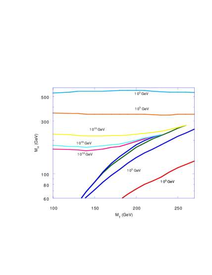
FIG. 2.: Perturbativity and stability bounds on the SM Higgs boson. $\Lambda$ denotes the energy scale where the particles become strongly interacting.

All of these corrections were included in Refs. [95] and [96], and reviewed in Ref. [97]. If one requires stability of the vacuum up to a scale $\Lambda$, then there is an excluded region in the Higgs mass-top mass plane. The result, for various values of $\Lambda$, is given in Figure 2. This figure, in addition, also includes the region excluded by the requirement that the scalar and Yukawa couplings remain perturbative by the scale $\Lambda$; these bounds will be discussed in the next section. The lower part of each curve is the vacuum stability bound; the upper part is the perturbation theory bound. The excluded region is outside the solid lines. Thus, for a top quark mass of 170 GeV, we see that a discovery of a Higgs boson with a mass of 90 GeV would imply that the standard model vacuum is unstable at a scale of $10^{5}$ GeV, i.e. if we live in a stable vacuum, the standard model must break down at a scale below $10^{5}$ GeV. The curves in Figure 2 are approximately straight lines in the vicinity of $M_{top}\sim 170$ GeV, thus the top mass dependence can be given analytically[97]. For $\Lambda=10^{19}$ GeV, we must have

$$M_{H}(GeV)\quad>\ 133+1.92(M_{top}(GeV)-175)-4.28{\alpha_{3}(M_{Z})-.12\over 0.006}$$ (36)

and for $\Lambda=1$ TeV,

$$M_{H}(GeV)\quad>\ 52+0.64(M_{top}(GeV)-175)-0.5{\alpha_{3}(M_{Z})-.12\over 0.006}$$ (37)

It is estimated[95, 97] that the error in the result, primarily due to the two-loop correction in the top quark pole mass and the effective potential, is less than $5$ GeV. In Figure 3, the stability and perturbation theory bounds are given explicitly as a function of $\Lambda$ for $M_{top}=175$ GeV.

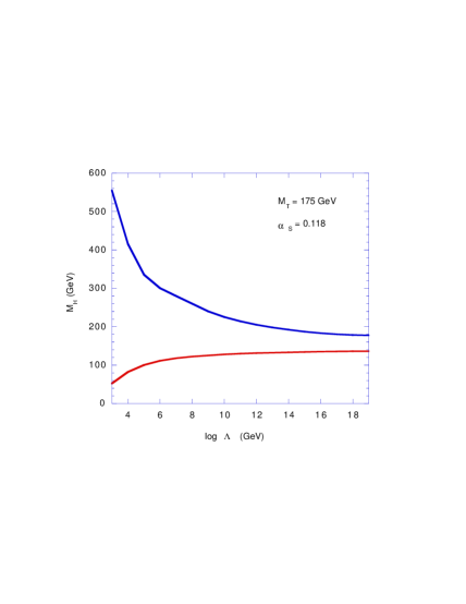
FIG. 3.: Perturbativity and stability bounds on the SM Higgs boson as a function of $\Lambda$ for $M_{top}=175$ GeV.

Of course, it is not formally necessary that we live in a stable vacuum. Should another deeper vacuum exist, it is only necessary that the Universe goes into our metastable vacuum and then stay there for at least 10 billion years. A detailed discussion of the finite temperature effective potential and tunnelling probabilities is beyond the scope of this review; the reader is referred to Refs. [95] and [97] for the details, as well as a comprehensive list of references. In short, the bound in the above paragraph for $\Lambda=10^{19}$ GeV weakens by $8$ GeV, and for $\Lambda=1$ TeV, weakens by about $25$ GeV. In all cases, the bound obtained by requiring that our vacuum have a lifetime in excess of 10 billion years is weaker than the bound obtained by requiring that the Universe arrive in our metastable vacuum.

We now turn to the question of vacuum stability for models with additional quarks and leptons.

3 Vacuum Stability Bounds and Four Generations

In this review, we are concentrating on two possibilities for quarks and leptons beyond the third generation: the chiral case and the vector-like case. In the latter case, the quarks and leptons cannot couple to Higgs doublets. They will thus have no effect on the vacuum stability bounds (except very weakly through their effects on the two-loop beta functions of the gauge couplings). We conclude that there are no vacuum stability bounds on the masses of vector-like quarks and leptons in models with Higgs doublets. Should one include a Higgs singlet, of course, then the vector-like quarks and leptons would couple, and a bound could be found on their masses which depends on the singlet Higgs mass as well as the fraction of the mass which comes from the singlet vev (since a bare mass is possible). There is one exception to this conclusion. As noted by Zheng[110], if one adds a vectorlike doublet and one or more vectorlike singlets, then Yukawa couplings can exist. He studied the stability bounds in that case (using the tree-level potential and one-loop beta functions), assuming that the Yukawa couplings were unity, and found that the bounds are much more stringent than in the three generation case—the lower bound from vacuum stability and the upper bound from perturbation theory come together at a scale well below the unification scale.

In the chiral case, more specific bounds can be found. It is clear from Eq. 23 that one can naively just replace the $h^{4}$ term with a summation over all quark and lepton Yukawa couplings. This amounts to replacing $M_{top}$ with

$$\left(M^{4}_{U}+M^{4}_{D}+{1\over 3}M^{4}_{E}+{1\over 3}M^{4}_{N}\right)^{1/4}$$ (38)

where $U$, $D$, $E$ and $N$ are additional $U$-type quarks, $D$-type quarks, charged leptons and neutrinos, respectively. The ${1\over 3}$ factor is a color factor. This replacement was noted by Babu and Ma[111] who simply rewrote Eq. 32 by substituting $M_{top}$ with the above expression (their paper was written when the top quark mass was believed to be 40 GeV, so the top mass was not included in the above.)

As discussed above, however, this procedure is not particularly accurate. A more detailed analysis, using one-loop beta functions, was carried out by Nielsen et al.[112] For simplicity, they assumed that the fourth generation fermions all had a common mass, $M_{4}$; since the quarks must have very similar mass, relaxing this assumption will not significantly affect the results. If one assumes that the standard model is valid up to $\Lambda\sim 10^{15}$ GeV, then they found that there is an upper bound on $M_{4}$ of only $110$ GeV. It is easy to see why this bound is so stringent. Suppose that $M_{4}$ were equal to $M_{top}$. Then the expression in the above paragraph(ignoring the leptons) would be $2M_{top}$, and thus the quark contribution would be $3M_{top}$. One might expect the bounds to be smaller by a factor of roughly $3$. In fact, it isn’t quite that severe since the upper line in the allowed region of Figure 2 is not significantly affected by the presence of additional generations. Nonetheless, the bound is quite stringent.

Nielsen et al.[112] argued that CDF bounds[113, 114] on stable, color triplets, as well as results from the successful description of top quark decays (which occur at the vertex), rule out $M_{4}$ up to $139$ GeV, and thus the standard model cannot be valid up to $10^{15}$ GeV. They found that new physics had to start below approximately $10^{10}$ GeV. However, this argument has a flaw. It is true that the CDF bounds on stable, color triplets rule out heavy quarks with decay lengths greater than a meter or so, and that the successful description of top quark decays rule out heavy quarks which decay at the vertex (at least up to about $150$ GeV), but there is still a window for decay lengths in which the quarks would have evaded detection. Depending on mixing angles, these decay lengths are quite plausible. Nonetheless, theirs is the most detailed analysis to date of the case in which $M_{4}$ is above $140$ GeV (and thus the scale of new physics is well below the unification scale).

A much more detailed analysis was carried out by Dooling et al.[115, 116] They performed a complete analysis, using the full, two-loop analysis of Casas, Espinosa and Quiros (discussed in the last section). They only consider the case in which the standard model is valid up to the unification scale, and thus only look at the case in which $M_{4}$ is very light, typically less than $120$ GeV. Their work is thus complimentary to that of Nielsen et al. They find that the point where the triviality bound and vacuum stability bound come together (see Figure 3) is (for $\Lambda\sim 10^{19}$ GeV) $M_{4}<110$ GeV. Thus, if the standard model is valid up to the unification scale, only a narrow region of masses still exists between the LEP lower bound (roughly 1/2 the center-of-mass energy) and the vacuum stability bound of $110$ GeV.

These works did assume that the quark and lepton masses were all degenerate with a mass $M_{4}$. If one relaxes this assumption, then one approximately can replace $(8/3)^{1/4}M_{4}$ with Eq. 38. Clearly it is easier to accommodate heavy leptons and neutrinos than heavy quarks.

Hung and Isidori[117] relaxed the assumption of a common $M_{4}$ and simply assumed a doublet of degenerate quartks with mass $M_{Q}$ and a doublet of degenerate leptons with mass $M_{L}$. They found that with $M_{L}\sim M_{W}$, $M_{Q}$ can be extended to 150 GeV before a Landau pole appears at the Planck mass. As $M_{L}$ is raised, $M_{Q}$ should correspondingly decrease if one requires that the Landau pole appear at or above the Planck mass.

C Perturbative Gauge Unification

The use of the RG equations as a tool to set bounds on and, in particlular, to “predict” particle masses is an “old” subject. The discussion on the bounds has been carried out in previous subsections. This subsection concentrates instead on the use of the RG equations to “predict” various masses. In particular, we shall pay special attention to the masses of any extra family of quarks and leptons. This analysis only works for chiral fermions. Vector-like fermions, having no Yukawa coupling to the SM Higgs field, will not have the desired influence on the evolution of the couplings as we shall see below.

In order to use the RG equations to make “predictions” on the masses, one has to invoke either some experimental necessities or some theoretical expectations -or rather prejudices- such as fixed points, gauge unification, etc. We shall describe below these concepts along with their consequences. To begin, we shall list the RG equations at two loops for the minimal SM with three generations [123].

$$16\pi^{2}\frac{d\lambda}{dt}= 24\lambda^{2}+4\lambda(3g_{t}^{2}-2.25g_{2}^{2}-0.45g_{1}^{2})$$ (43)

$$-6g_{t}^{4}+(16\pi^{2})^{-1}\{30g_{t}^{6}$$

$$-[3g_{t}^{4}+2g_{l}^{4}-80g_{3}^{2}g_{t}^{2}]\lambda$$

$$-144\lambda^{2}g_{t}^{2}-312\lambda^{3}-32g_{3}^{2}g_{t}^{4}\}$$

$$16\pi^{2}\frac{dg_{t}^{2}}{dt}= g_{t}^{2}\{9g_{t}^{2}-16g_{3}^{2}-4.5g_{2}^{2}-1.7g_{1}^{2}+$$ (46)

$$(8\pi^{2})^{-1}[-12g_{t}^{4}+6\lambda^{2}+g_{t}^{2}$$

$$(-12\lambda+36g_{3}^{2})-108g_{3}^{4}]\}$$

$$16\pi^{2}\frac{dg_{1}^{2}}{dt}= g_{1}^{4}\{(41/5)+(16\pi^{2})^{-1}[(199/25)g_{1}^{2}+(27/5)g_{2}^{2}+$$ (48)

$$(88/5)g_{3}^{2}-(17/5)g_{t}^{2}]\}$$

$$16\pi^{2}\frac{dg_{2}^{2}}{dt}= g_{2}^{4}\{-(19/3)+(16\pi^{2})^{-1}[(9/5)g_{1}^{2}+(35/3)g_{2}^{2}+$$ (50)

$$24g_{3}^{2}-3g_{t}^{2}]\}$$

$$16\pi^{2}\frac{dg_{3}^{2}}{dt}= g_{3}^{4}\{-14+(16\pi^{2})^{-1}[(11/5)g_{1}^{2}+9g_{2}^{2}$$ (52)

$$-52g_{3}^{2}-4g_{t}^{2}]\}$$

To set the notations straight, our definition of $g_{1}$ uses the $SU(5)$ convention and is related to the $U(1)_{Y}$ coupling $g^{\prime}$ by $g_{1}=\sqrt{3/5}g^{\prime}$. In the evolution of these couplings we will neglect the contributions coming from the lighter fermions.

In the above RG equations, clearly the important couplings are those of the top quark Yukawa and of the Higgs quartic couplings, and, to a certain extent, also the QCD coupling. As we have seen earlier, one important use of such equations is by following the evolution of $\lambda$ with the initial value of $g_{t}$ fixed by its experimental value. Requiring $\lambda$ to be positive (for vacuum stability reason) at least up to the Planck scale allows us to set a lower limit on the Higgs mass to be $\sim$ 136 GeV. This use of the RG equations is rather solid in the sense that it relies only on the vacuum stability criterion of quantum field theory. Other uses which are discussed below are more speculative but are quite interesting in that several predictions can be made and can be tested.

In dealing with RG equations, a natural question that comes to mind is whether or not there exist stable fixed points. Basically, a stable fixed point is a point in coupling space to which various couplings converge regardless of their initial values. This is an attractive idea that has wide applications in many fields of physics, such as critical phenomena- to mention just one of many. In particle physics, there were many speculations concerning the nature of such fixed points if they truly exist. For example, Gell-Mann and Low [124], and subsequently, Johnson, Wiley and Baker [125] have speculated that quantum electrodynamics might possess an ultraviolet stable fixed point which will render QED finite. Other more “recent” speculations dealt with the very interesting subject of the origin of particle masses- at least of the heavy one(s).

In general, a stable fixed point appears as a zero of the $\beta$ function which would be meaningful only if one has a full knowledge of such a function. In the absence of such a knowledge, one might have to resort to approximations allowed by perturbation theory. In regions where various couplings can be considered to be “small” enough so that the use of one or two-loop $\beta$ functions might be justified, one would try to “run” the couplings over a large region of energy and see if they converge to a point for arbitrary initial values. If such a point is found, say by a numerical study of the RG equations, one would qualify this as a fixed point. Such an approach has been pioneered by Pendlenton and Ross [126], and, in particular by Hill [127], where the fixed points are of the infrared nature. Of relevance to this report is the suggestion by various authors that a fourth generation might be needed for the existence of such a fixed point.

Let us first summarize what has been done for the top quark mass and subsequently describe works related to the masses of a fourth generation.

Pendleton and Ross [126] were the first to suggest a relationship between the top quark Yukawa coupling and the QCD coupling as a result of an infrared (IR) stable fixed point. To see this, one can combine the one-loop RG equations for $g_{t}$ and the QCD coupling $g_{3}$ (first terms on the right-hand side of Eq. (38)) to form a RG equation for the ratio $g_{t}/g_{3}$, namely

$$16\pi^{2}\frac{d(g_{t}/g_{3})}{dt}=\frac{9}{2}g_{t}^{2}-g_{3}^{2}-\frac{3}{4}(3g^{2}+g^{\prime 2})-\frac{2}{3}g^{\prime 2}.$$ (53)

Ignoring the electroweak contributions in Eq. (39), there is an IR fixed point obtained by setting the right-hand side to zero. Pendleton and Ross obtained a relation

$$g_{t}^{2}=g_{t,irs}^{2}=\frac{2}{9}g_{3}^{2}.$$ (54)

It turns out that the above relation gives too low of a mass for the top quark. In fact, the original prediction [126] using Eq. (40) and a value of $\alpha_{3}=g_{3}^{2}/4\pi\sim 1/7$ (at a scale of $\sim 2M_{W}$) gives a mass of $\sim$ 110 GeV. Using the current value of $\alpha_{3}\approx 0.12$ (at the Z mass), the prediction would have been even lower, even after electroweak corrections are included. It goes without saying that this cannot be true for we already know that the top quark mass is $\sim$ 175 GeV. As pointed out by Hill [127] long before the discovery of the top quark, the Pendleton-Ross fixed point is only a quasi fixed point in the sense that it can never be reached at the scale of interest $\sim$ 100 GeV. Hill proposed an intermediate fixed point that can be found by setting the $\beta$ function in the RG for $g_{t}$ to zero with a “slowly varying” $g_{3}$ replaced by a constant taken to be some average value between two scales: 100 GeV and $10^{15}$ GeV. This translates into an approximate relation

$$\frac{9}{2}g_{t}^{2}\approx 8\bar{g_{3}}^{2},$$ (55)

With $\bar{g_{3}}^{2}\sim 0.7$, Hill made the prediction for the top quark mass to be $\approx$ 240 GeV. This is now known to be much too large, although at the time the prediction was made, it appeared to be a plausible value.

In the above discussion for the top quark mass as a result of an IR stable fixed point, one feature clearly emerges: a heavy fermion is needed to drive the evolution toward a fixed point. This point was made even clearer in a detailed study of Bagger, Dimopoulos and Massó [128]. These authors made two assumptions: the first one is the existence of a desert between the weak scale $M_{W}$ and some Grand Unified scale $M_{X}\sim 10^{15}$ GeV and the second one being that of perturbative unification. The question asked in Ref. [128] was the following: what should the initial values of various Yukawa couplings at $M_{X}$ be in order for those couplings to reach the fixed in a “physical time” $t_{W}=\frac{1}{16\pi^{2}}\ln(\frac{M_{X}}{M_{W}})\sim 1/5$? Again, it turns out that “large” initial values (at $M_{X}$) of Yukawa couplings guarantee that the fixed point is reached in “physical time”. What is this fixed point and what does it say about masses of possible extra generations if they exist? We shall describe below the salient points of the analysis of Ref. [128].

We begin the discussion of Ref. [128] with the following one-loop RG equations for the quark and lepton Yukawa couplings:

$$\frac{dT_{Q}}{dt}=2(G_{Q}-T)T_{Q}-3Tr(S_{U}^{2}),$$ (57)

$$\frac{dT_{L}}{dt}=2(G_{L}-T)T_{L}-3Tr(S_{E}^{2}),$$ (58)

where various Yukawa factors are defined as $T_{Y}=Tr(Y^{{\dagger}}Y)$ with $Y=U,D,E$ or $N$, $T_{Q}=T_{U}+T_{D}$, $T_{L}=T_{E}+T_{N}$, $T=3T_{Q}+T_{L}$, $S_{U}=U^{{\dagger}}U-D^{{\dagger}}D$ and $S_{E}=E^{{\dagger}}E-N^{{\dagger}}N$. Finally the gauge factors $G$’s are defined as $G_{U}=G_{D}=G_{Q}=8g_{3}^{2}+\frac{9}{4}g_{2}^{2}$ and $G_{E}=G_{N}=G_{L}=\frac{9}{4}g_{2}^{2}$ where the contribution from $g_{1}$ has been neglected. Notice that $t=\frac{1}{16\pi^{2}}\ln(\frac{M_{X}}{M})$.

FIG. 4.: (a) The trace $T_{Q}$ at $M_{W}$ as a function of the trace $T_{Q}$ and $M_{X}$ for $N_{F}=8$ and $T_{L}=0$. The dotted line denotes the radial quark fixed point. For $T_{Q}(M_{X})>0.1$, the fixed point is reached in physical time. (b)$T_{L}(M_{W})$ as a function of $T_{L}(M_{X})$ for $N_{F}=8$ and $T_{Q}=0$.

To simplify the discussion, Ref. [128] first assumed degenerate quarks and degenerate leptons so that $S_{U}=0$ as well as $S_{E}=0$. If the gauge couplings can be approximated as constant (or very slowly varying), $G_{Q}$ and $G_{L}$ in Eqs. (42) can be replaced by some averages similar to the procedure used by Hill [127]. Let us denote these averages by $\bar{G_{Q}}$ and $\bar{G_{L}}$. It is then easy to see that Eqs.(42) have the following two distinct fixed points: $\bar{G_{Q}}=T$ (quark radial fixed point) and $\bar{G_{L}}=T$ (lepton radial fixed point). Whether or not these fixed points are reached will depend on the initial values of $T_{Q}$ or $T_{L}$ at the Grand Unified scale $M_{X}$. If $T(M_{X})$ is below some critical value $T(M_{X})_{min}$, the fixed point $\bar{G}$ will not be reached in “physical time” $t\sim 1/5$: the value of $T$ at $M_{W}$ will be less than the fixed point value $\bar{G}=T$. This fact has allowed Ref. [128] to set an upper limit on heavy fermion masses with the upper limit being the IR stable fixed point. Setting $S_{Y}=T_{L}=0$, Ref. [128] plotted $T_{Q}$ at the weak scale as a function of its value at $M_{X}$. This is shown in Fig. 4a. The result for the lepton case is shown in Fig. 4b.

The figure shows the result for eight families. We are, of course, concerned only with four families which are still allowed. within error, by precision electroweak results. For four families, Ref. [128] gave the following upper bounds on $T$:

$$T_{Q}\lesssim 2.7,$$ (60)

$$T_{L}\lesssim 3.4.$$ (61)

(The above numbers used values of gauge couplings which are now outdated.) This translates into the following distinct bounds on fermion masses for four families:

$$\Sigma M_{Q}^{2}\lesssim(290\,GeV)^{2},$$ (63)

$$\Sigma M_{L}^{2}\lesssim(325\,GeV)^{2}.$$ (64)

(These bounds would be slightly less if recent values of the gauge couplings are used.) The above bound for the quarks, for example, would translate roughly into a bound on the mass of a degenerate fourth generation quark (after subtracting out the top quark) as $M_{U,D}\lesssim$ 164 GeV. Is this what one should be aiming for when one tries to look for fourth-generation quarks?

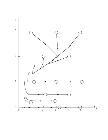
FIG. 5.: Flow of $\lambda$ and $g_{t}$ towards fixed points in the standard one-Higgs doublet model. Open circles denote initial points. Crosses denote final fixed points.

Hill, Leung and Rao [129] made an extensive study of the RG fixed points and their connections with the mass of the Higgs boson(s) for the one-Higgs doublet and the two-Higgs doublet cases, and for up to five generations. In this work, the Higgs quartic coupling(s) is run simultaneously with the various Yukawa couplings and, as a result, one clearly sees again the interplay between heavy fermions and the Higgs field. This is shown for example in Figs. 1 and 2 of Ref. [129] for the one-Higgs doublet case with three generations, which are reproduced in Figs. 5 and 6.

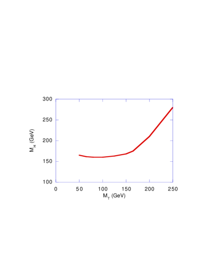
FIG. 6.: Relation between the Higgs mass and the top quark mass in the standard one-Higgs model.

Other attempts of using the RG fixed points to construct fermion mass matrices have been made, for example in Ref. [153]. However the “predicted” value for the top quark mass is now outdated.

A different approach was taken by one of us (P.Q.H.) [65] concerning the influence of a possible fourth generation on the evolution of all couplings of the SM and not merely the Yukawa couplings. In particular, the question that was asked was whether or not there can be gauge unification in the nonsupersymmetric SM and under which conditions this can be achieved. As we shall see below, it turns out that a fourth family of chiral fermions will be needed and that their masses are found to be fairly constrained.

The possibility of coupling-constant unification of the three gauge interactions of the Standard Model (SM) is, without any doubt, one of the most important issues in particle physics. Coupling-constant unification is a necessary, but not sufficient, condition for a Grand Unification of the SM [131, 132, 133]. Such a possibility is particularly attractive since it would provide a unified explanation for a number of puzzling features of the SM such as electric charge quantization for example.

There are various ways that the three gauge couplings can get unified. The simplest way is to assume that there is a “desert” (i.e. no new physics) between the electroweak scale and the scale at which unification occurs. Simply speaking, the three gauge couplings are left to evolve beyond the electroweak scale under the assumption that there is no additional gauge interactions of the type which would modify the evolution of some of the gauge couplings. A more complicated way would be to assume that there is one or several intermediate scales where partial unification among two of the three couplings occurs. This might well be the case. However we shall restrict ourselves, in this report, to the simplest scenario of unification with a “desert” and search for conditions under which this can be achieved. This was the approach taken by one of us (P. Q. H.) [65].

We will proceed in two steps. First, we will present the evolution of the gauge couplings and show the places where they cross, ignoring any heavy threshold effects that might be- and should be if there truly is unification- present. In this discussion, we will show both the minimal SM with three generations and the one with an extra fourth generation. We shall see that, under certain restrictions on the masses (fourth generation and Higgs masses), the latter possibility provides a better “convergence” of the three gauge couplings. By convergence under the quotation marks, we mean that they do not precisely meet at the same point. The “true” convergence will be shown to be accomplished by the inclusion of heavy threshold effects. In fact it would be senseless to claim unification without taking into account such effects.

We first summarize the situation with three families.

The first task is to integrate Eq.(38) numerically and look for the places where the couplings meet, disregarding for the moment the possibility that there might be unification. We then have to set up some kind of criteria to decide on how close to each other all three couplings have to be in order for them to have a chance of actually converging to a single scale, once heavy particle thresholds, such as those of the X and Y bosons of $SU(5)$ for instance, are taken into account. Once these criteria are satisfied and heavy particle threshold effects are included, one can put an error on the unification scale and, consequently, an error on the proton lifetime.

Fig. 7 shows the evolution, without heavy threshold effects, of $g_{3}$, $g_{2}$, and $g_{1}$ of $SU(3)\otimes SU(2)\otimes U(1)$ for the case with three generations. Clearly these three couplings do not converge.

FIG. 7.: Evolution of couplings in the three generation case.

The question is: How far apart are they from each other and at what scales? As far as the scales are concerned, we will be interested only in those which are above some minimum value implied by the lower bound on proton decay. A rough estimate of that lower bound is obtained by noticing that $\tau_{p\rightarrow e^{+}\pi^{0}}(yr)\approx 10^{31}(M_{G}/4.6\times 10^{14})^{4}$. This gives $M_{G}\gtrsim 1.3\times 10^{15}$ GeV (corresponding to $\ln(E/175)=29.64$ on the graph) for $\tau_{p\rightarrow e^{+}\pi^{0}}(yr)\gtrsim 5.5\times 10^{32}$. The next question is the following: Starting from $M_{G}^{min}\sim 1.3\times 10^{15}$ GeV, how far apart are the three gauge couplings from each other at a given energy scale? As stated above, the reason for asking such a question stems from the fact that, if the SM were to be embedded at $M_{G}$ in a Grand Unified model such as $SU(5)$ [132] (for instance), the decoupling of various heavy GUT particles would shift the three couplings from a common $\alpha_{G}$ to (possibly) different values. As shown below, for a wide range of “reasonable” heavy particle masses, such an effect produces no more than $\sim$ 5% shift from the common value and in the same direction. It turns out that the modified couplings can differ by no more than $\sim$ 4%. From this a reasonable criterion would be to require that, at a scale $M_{G}\geq m_{G}^{min}$, the three gauge couplings are within 4% of each other.

We shall take $SU(5)$ [132] as a prototype of a Grand Unified Theory. Let us assume the following heavy particle spectrum:$(X,Y)=(\bar{3},2,5/6)+c.c.$ with mass $M_{V}$, real scalars $(8,1,0)+(1,3,1)+(1,1,0)$ (belonging to the 24-dimensional Higgs field) with mass $M_{24}$, and the complex scalars $(3,1,-1/3)$ (belonging to the 5-dimensional Higgs field), with mass $M_{5}$. (The quantum numbers are with respect to $SU(3)\otimes SU(2)\otimes U(1)$.) The heavy threshold corrections are then [134]:

$$\Delta_{1}=\frac{35}{4\pi}\ln(\frac{M_{G}}{M_{V}})-\frac{1}{30\pi}\ln(\frac{M_{G}}{M_{5}})+\Delta^{NRO}_{1},$$ (66)

$$\Delta_{2}=-\frac{1}{6\pi}+\frac{21}{4\pi}\ln(\frac{M_{G}}{M_{V}})-\frac{1}{6\pi}\ln(\frac{M_{G}}{M_{24}})+\Delta^{NRO}_{2},$$ (67)

$$\Delta_{3}=-\frac{1}{4\pi}+\frac{7}{2\pi}\ln(\frac{M_{G}}{M_{V}})-\frac{1}{12\pi}\ln(\frac{M_{G}}{M_{5}})-\frac{1}{4\pi}\ln(\frac{M_{G}}{M_{24}})+\Delta^{NRO}_{3},$$ (68)

where

$$\Delta^{NRO}_{i}=-\eta k_{i}(\frac{2}{25\pi\alpha_{G}^{3}})^{1/2}\frac{M_{G}}{M_{Planck}},$$ (69)

with $k_{i}=1/2,3/2,-1$ for $i=1,2,3$, is the correction coming from possible dimension 5 operators present between $M_{G}$ and $M_{Planck}$. The modified gauge couplings can be expressed in terms of the unified coupling $\alpha_{G}$ (at $M_{G}$) as:

$$\alpha_{i}(M_{G})=\frac{\alpha_{G}}{1-\alpha_{G}\,\Delta_{i}},$$ (70)

where $i=1,2,3$. We then define the fractional difference between the modified gauge couplings as:

$$d_{ij}=\frac{\alpha_{i}-\alpha_{j}}{\alpha_{i}},$$ (71)

for $i,j=1,2,3$ and the definition refers to $\alpha_{i}$ as being the larger of the two couplings. For a wide range of heavy particle masses (in relation with $M_{G}$) and the parameter $\eta$ appearing in $\Delta_{i}$, and for $\alpha_{G}\sim 0.024-0.028$, it is straightforward to see that $d_{ij}$ can be at most 4% [65]. ¿From this simple analysis, one can reasonably set a criterion for a given scenario to have a chance of having gauge coupling unification: the fractional difference among the three gauge couplings at some scale $M_{G}\geq M_{G}^{min}$ should not exceed 4%.

For the SM with three generations and taking into account the presence of $M_{G}^{min}\sim 1.3\times 10^{15}$ GeV, one finds the following trend: $d_{32}$ decreases from 3% as one increases the energy scale beyond $M_{G}^{min}$, while $d_{31}$ increases from 4% and $d_{21}$ also increases from 7%. (For example, at $M_{G}\sim 3.3\times 10^{15}$ GeV, $d_{32}\sim$ 1.4%, $d_{31}\sim$ 8.4% and $d_{21}\sim$ 9.7%. ¿From these considerations- and not from just “eyeballing” the curves- one might conclude that the minimal SM with three generations does indeed have some problem with unification of the gauge couplings.

There is a drastic change to the whole scenario when one postulates the existence of a fourth generation of quarks and leptons [65]. The main reason is the fact that the Yukawa contributions to the running of the gauge couplings appear at two loops. In the three generation case, the top Yukawa coupling actually decreases sligthly with energy because its initial value is partially cancelled by the QCD contribution (at one loop). As a result, the presence of a heavy top quark is insignificant in the evolution of the gauge couplings at high energies when there are only three generations. The presence of more than three generations drastically modifies the evolution of the Yukawa, Higgs quartic self-coupling, and the three gauge couplings. For example, with a fourth generation which is sufficiently heavy, all Yukawa couplings grow with energy, significantly affecting the evolution of the gauge couplings. It turns out, as we shall see below, that the Yukawa couplings can develop Landau poles below the Planck scale. If there were any possibility of gauge unification, one would like to ensure that it occurs in an energy region where perturbation theory is still valid. Furthermore, the unification scale will have to be greater than $M_{G}^{min}$ (as discussed above). As we shall see, the validity of perturbation theory plus the lower bound on the proton lifetime put a severe constraint on the masses of the fourth generation.

The two-loop renormalization group equations applicable to four generations are given by [123, 65]:

$$16\pi^{2}\frac{d\lambda}{dt}= 24\lambda^{2}+4\lambda(3g_{t}^{2}+6g_{q}^{2}+2g_{l}^{2}-2.25g_{2}^{2}-0.45g_{1}^{2})$$ (77)

$$-2(3g_{t}^{4}+6g_{q}^{4}+2g_{l}^{4})+(16\pi^{2})^{-1}\{30g_{t}^{6}$$

$$+48g_{q}^{6}+16g_{l}^{6}-[3g_{t}^{4}+6g_{q}^{4}+2g_{l}^{4}-80g_{3}^{2}(g_{t}^{2}$$

$$+2g_{q}^{2})]\lambda-6\lambda^{2}(24g_{t}^{2}+48g_{q}^{2}+16g_{l}^{2})-312\lambda^{3}$$

$$-32g_{3}^{2}(g_{t}^{4}+2g_{q}^{4})\}$$

$$16\pi^{2}\frac{dg_{t}^{2}}{dt}= g_{t}^{2}\{9g_{t}^{2}+12g_{q}^{2}+4g_{l}^{2}-16g_{3}^{2}-4.5g_{2}^{2}-1.7g_{1}^{2}+$$ (81)

$$(8\pi^{2})^{-1}[1.5g_{t}^{4}-2.25g_{t}^{2}(6g_{q}^{2}+3g_{t}^{2}+2g_{l}^{2})$$

$$-12g_{q}^{4}-(27/4)g_{t}^{4}-3g_{l}^{4}+6\lambda^{2}+g_{t}^{2}$$

$$(-12\lambda+36g_{3}^{2})-(892/9)g_{3}^{4}]\}$$

$$16\pi^{2}\frac{dg_{q}^{2}}{dt}= g_{q}^{2}\{6g_{t}^{2}+12g_{q}^{2}+4g_{l}^{2}-16g_{3}^{2}-4.5g_{2}^{2}-1.7g_{1}^{2}+$$ (85)

$$(8\pi^{2})^{-1}[3g_{q}^{4}-g_{q}^{2}(6g_{q}^{2}+3g_{t}^{2}+2g_{l}^{2})$$

$$-12g_{q}^{4}-(27/4)g_{t}^{4}-3g_{l}^{4}+6\lambda^{2}+g_{q}^{2}$$

$$(-16\lambda+40g_{3}^{2})-(892/9)g_{3}^{4}]\}$$

$$16\pi^{2}\frac{dg_{l}^{2}}{dt}= g_{l}^{2}\{6g_{t}^{2}+12g_{q}^{2}+4g_{l}^{2}-4.5(g_{2}^{2}+g_{1}^{2})+$$ (88)

$$(8\pi^{2})^{-1}[3g_{q}^{4}-g_{q}^{2}(6g_{q}^{2}+3g_{t}^{2}+2g_{l}^{2})-12g_{q}^{4}$$

$$-(27/4)g_{t}^{4}-3g_{l}^{4}+6\lambda^{2}-16\lambda g_{l}^{2}]\}$$

$$16\pi^{2}\frac{dg_{1}^{2}}{dt}= g_{1}^{4}\{(163/15)+(16\pi^{2})^{-1}[(787/75)g_{1}^{2}+6.6g_{2}^{2}+$$ (90)

$$(352/15)g_{3}^{2}-3.4g_{t}^{2}-4.4g_{q}^{2}-3.6g_{l}^{2}]\}$$

$$16\pi^{2}\frac{dg_{2}^{2}}{dt}= g_{2}^{4}\{-(11/3)+(16\pi^{2})^{-1}[2.2g_{1}^{2}+(133/3)g_{2}^{2}+$$ (92)

$$32g_{3}^{2}-3g_{t}^{2}-3g_{q}^{2}-2g_{l}^{2}]\}$$

$$16\pi^{2}\frac{dg_{3}^{2}}{dt}= g_{3}^{4}\{-(34/3)+(16\pi^{2})^{-1}[(44/15)g_{1}^{2}+12g_{2}^{2}$$ (94)

$$-(4/3)g_{3}^{2}-4g_{t}^{2}-8g_{q}^{2}]\}.$$

For simplicity, we have made the following assumptions: a Dirac mass for the fourth neutrino and the quarks and leptons of the fourth generation are degenerate $SU(2)_{L}$ doublets. The respective Yukawa couplings are denoted by $g_{q}$ and $g_{l}$ respectively. Also, in the evolution of the quartic coupling $\lambda$ and the Yukawa couplings, we will neglect the contributions of $\tau$ and bottom Yukawa couplings, as well as the electroweak gauge couplings, $g_{1}$ and $g_{2}$, to the two-loop $\beta$ functions since they are not important. Also, as long as the mixing between the fourth generation and the other three is small, one can neglect such a mixing.

In the numerical analysis given below we shall fix the mass of the top quark to be 175 GeV. We shall furthermore restrict the range of masses of the fourth generation so that the Landau poles lie comfortably above $10^{15}$ GeV, in such a way that unification occurs at a scale which would guarantee the validity of perturbation theory as well as satisfying the lower bound on the proton lifetime. Concerning the former requirement, it basically says that one should look at unification scales where the values of the Higgs quartic and Yukawa coulings are still sufficiently perturbative that one can neglect contibutions coming from three-loop (and higher) terms to the $\beta$ functions.

Fig. 8 shows $g_{1}^{2}$, $g_{2}^{2}$ and $g_{3}^{2}$ as a function of energy for a particular set of masses: $m_{Q}=151$ GeV, $m_{L}=95.3$ GeV, where $m_{Q}$ and $m_{L}$ denote the fourth generation quark and lepton masses respectively.

FIG. 8.: Couplings as a function of energy for the set of masses given in the text.

It is already well known, from the discussion in the previous section, that, by adding more heavy fermions, the vacuum will tend to be destabilized unless the Higgs mass is large enough. As we have seen, the vacuum stability requirement is equivalent to the restriction $\lambda>0$. Furthermore, the heavier the Higgs boson is, above a minimum mass that ensures vacuum stability, the lower (in energy scale) the Landau pole turns out to be. It turns out that this Landau pole should not be too far from $M_{G}^{min}$ otherwise $g_{3}$, $g_{2}$ and $g_{1}$ would not come close enough to each other. On the other hand, it should not be too close either because of the requirement of the validity of perturbation theory. These considerations combine to give a prediction of the Higgs mass, namely $m_{H}=188$ GeV for the above values of the fourth generation masses [65]. The dependance of the Higgs mass on the fourth generation mass in this analysis is obviously striking.

Following the criteria that we have set for taking into account the heavy threshold effects, the midified couplings $\tilde{\alpha}_{i}(M_{G})$ expressed in terms of $\alpha_{i}(M_{G})$ (which can be read off from the graph) and the threshold correction factors $\Delta_{i}$ are given by: $1/\tilde{\alpha}_{i}(M_{G})=1/\alpha_{i}(M_{G})+\Delta_{i}$. The choice of the mass scales $M_{5}$, $M_{24}$, $M_{V}$, and the parameter $\eta$ is arbitrary and is only fixed to a certain extent by the requirement that $\tilde{\alpha}_{i}(M_{G})$’s should be as close to each other as the precision allows. As an example, the choice $M_{5}=M_{G}$, $M_{24}=M_{G}$, $M_{V}=0.5M_{G}$ and $\eta=10$ (where we have picked $M_{G}\approx 3.5\times 10^{15}$ GeV) transforms $\alpha_{3}(M_{G})=0.0278$, $\alpha_{2}(M_{G})=0.0273$ and $\alpha_{1}(M_{G})=0.0285$ (values that can be read off Fig. (8)) to $\tilde{\alpha}_{3}(M_{G})=0.02735$, $\tilde{\alpha}_{2}(M_{G})=0.02662$ and $\tilde{\alpha}_{1}(M_{G})=0.02705$. From these values, one can conclude that the couplings are practically the same with all three equal to $\alpha_{G}\approx 0.027$ or $1/\alpha_{G}\approx 37$.

The above simple exercise simply shows that, with just an additional fourth generation having a quark mass $m_{Q}\approx 151$ GeV, a lepton mass $m_{L}\approx 95.3$ GeV and a Higgs mass $m_{H}\approx 188$ GeV, unification of all three gauge couplings in the nonsupersymmetric SM can be achieved after one properly takes into account threshold effects from heavy GUT particles [65]. Other combinations of masses are possible for gauge unification but their values will not be much different from the quoted ones, the reason being the requirement that the mass range of the fourth generation be restricted to one that will have Landau poles only above $10^{15}$ GeV. Do the masses given above satisfy the requirement of perturbation theory? In fact, at the unification point $M_{G}=3.5\times 10^{15}$ GeV, one has (with $\alpha_{i}\equiv g_{i}^{2}/4\pi$): $\alpha_{t}=0.4$, $\alpha_{q}=0..16$, $\alpha_{l}=0.48$ and $\lambda/4\pi=0.19$. Although these values are not “small”, they nevertheless satisfy the requirements of perturbation theory, namely $\alpha_{t,q,l}\lesssim 1$ and $\lambda/4\pi\lesssim 0.4$. (The latter requirement comes from lattice calculations which put an upper bound on the Higgs mass of $\sim$ 750 GeV.) For comparison, $\alpha_{t}$ in the three-family SM has a value of 0.016 at a comparable scale and this explains why it is unimportnat in the evolution of the SM gauge couplings.

An important consequence of a fourth generation in bringing about gauge unification is the value of the unification scale itself. In the example given above, it is $M_{G}=3.5\times 10^{15}$ GeV [65]. In the nonsupersymmetric SU(5) model, the dominant decay mode ofthe proton is $p\rightarrow e^{+}\pi^{0}$ and the mean partial lifetime is $\tau_{p\rightarrow e^{+}\pi^{0}}(yr)\approx 10^{31}(M_{G}/4.6\times 10^{14})^{4}$. Taking into account various uncertainties such as heavy threshold effects, hadronic matrix elements, etc., the predicted lifetime is $\tau_{p\rightarrow e^{+}\pi^{0}}(yr)\approx 3.3\times 10^{34\pm 2}$ to be compared with $\tau_{p\rightarrow e^{+}\pi^{0}}^{exp}(yr)>5.5\times 10^{32}$ [65]. Notice that the central value is within reach of the next generation of SuperKamiokande proton decay search.

Another hint on the masses of a fourth generation comes from considerations of models of dynamical symmetry breaking à la top-condensate[46] This will be discussed in Section 5 where one can see how the original idea of using the top quark as the sole agent for electroweak symmetry breaking (in the form of $t\bar{t}$ condensates) led to a prediction for the top quark mass (before its discovery) to be much larger than its experimental value. The original form of this attractive idea obviously has to be modified, most likely by the introduction of new fermions such as a fourth generation or $SU(2)$-singlet quarks.

In the above discussion on perturbative gauge unification, as well as in the subsequent related discussion in Section V, the issue of the gauge hierarchy problem is not considered. Such an issue is beyond the scope of the largely phenomenological approach that we are taking. This point was alluded to in our Introduction where we stressed that none of the reasons given for considering quarks and leptons beyond the third generation is fully compelling, but each, including the one on perturbative gauge unification, is suggestive. It is certainly possible that the “solution” of the gauge hierarchy problem will not affect the above arguments; the recently developed alternative to supersymmetry and technicolor, TeV-scale gravity, for example, may not appreciably change results on gauge unification. A full consideration of the gauge hierarchy problem is beyond the scope of this review.

D Mixing Angles

In previous sections, we have seen that the masses of quarks and leptons, although arbitrary, are constrained by phenomenological considerations as well as vacuum stability and perturbation theory. The mixing angles of quarks and leptons are also arbitrary, however there are no constraints from vacuum stability and perturbation theory (and only weak phenomenological constraints). Thus, a much wider range of mixing angles can be accommodated, and one can only be guided by considering various models for these angles. In this section, we will discuss plausible models for mixing angles. Since we know that the quark sector has nonzero mixing angles, but that the lepton sector may not, we will first look at the lepton sector, and then the quark sector.

1 Leptons

The only phenomenological indication of any mixing in the lepton sector comes from neutrino oscillations. At the time of this writing, there are three indications of oscillations: solar neutrinos[135], atmospheric neutrinos[136] and LSND[137]. It is difficult, although not quite impossible, to reconcile all three of these in a three generation model. If there are four light neutrinos, in this case, the fourth neutrino must be sterile (an isosinglet) in order to avoid the bounds from LEP. Such a neutrino could exist without requiring the existence of any additional fermions. It is likely that the situation will be clarified within a year or so at Superkamiokande and the Solar Neutrino Observatory. A detailed discussion of neutrino oscillations and their phenomenology, including the recent strong evidence for atmospheric neutrino oscillations at SuperKamiokande, can be found in Ref. [138]. We will defer to that review in this paper, and will not discuss the possibility of light isosinglet neutrinos further.

We certainly will, however, discuss the case in which a fourth generation neutrino is very heavy. This will automatically occur if the fourth generation is vectorlike. Even if it is chiral, models exist that can give such a mass. Recently, one of us[139] has considered a model of neutrino masses with four generations where one can obtain dynamically one heavy fourth generation and three light, quasi-degenerate neutrinos. Ref. [140] has also considered a scenario with four generations which has similar consequences.

Suppose that the heavy leptons form a standard chiral family, with a right-handed neutrino. The bounds from the $Z$ width obtained at LEP force the mass of the $N$ and $E$ to be greater than 45 GeV. Are there any phenomenological bounds on the mixing? In analogy with the quark sector (as well as the prejudice from most models), one expects the mixing to be the greatest between the third and fourth generations. This will affect the $\tau\nu_{\tau}W$ vertex, multiplying it by $\cos\theta$, where $\theta$ is the mixing angle. Since all $\tau$ decays occur through this vertex, the result will be a suppression in the overall rates. For some time, it was believed that the mass of the $\tau$ was $1782\pm 2$ MeV, and the measured rate was too low; mixing with a fourth generation was a straightforward explanation[141, 142, 143]. However, the $\tau$ mass has now been measured to much higher precision at BES[144] to be $1776.96\pm 0.2\pm 0.2$ MeV, and the measured rate is now in agreement with theoretical expectations. This has been analyzed by Swain and Taylor[145, 146], who find a model-independent bound on the mixing of $\sin^{2}\theta<0.007$. A similar bound can be obtained for mixing between the fourth generation and the first two, although one expects those angles to be smaller.

What values of the mixing might one expect? There are four plausible (in the view of the authors, of course) values of the mixing angle between the third and fourth generations: $(a)\sin^{2}\theta=m_{\tau}/m_{E}\quad(b)\sin^{2}\theta=m_{\nu_{\tau}}/m_{N}\quad(c)\sin^{2}\theta=m_{W}^{2}/m_{Pl}^{2}\quad(d)\sin^{2}\theta=0$

The first of these occurs in typical see-saw models. The second occurs in models in which the mixing occurs only in the neutrino mass matrix. The third occurs in models with a global or discrete lepton-family symmetry broken by Planck scale effects, and the fourth occurs when the symmetry is not broken by Planck scale effects. We now discuss each of these.

The first relation, $\sin^{2}\theta=m_{\tau}/m_{E}$, occurs in models in which the $2\times 2$ mass sub-matrices are of the form $\pmatrix{0&A\cr A&B\cr}$. If the neutrino and charged lepton mass matrices are of that form, then the mixing angle is given by $\sqrt{m_{\tau}/m_{E}}-\sqrt{m_{\nu_{\tau}}/m_{N}}$, which gives $\sin^{2}\theta=m_{\tau}/m_{E}$ for realistic values of the $\nu_{\tau}$ mass. Models of this type were pioneered by Weinberg[147] and Fritzsch[148], who noticed that they will give the successful relation for the Cabibbo angle: $\sin^{2}\theta_{c}=m_{d}/m_{s}$. Fritzsch also showed[149] that there are some very simple symmetries which automatically give this relation. When the rate for leptonic decays was believed to be too low, Fritzsch[150] used this relation to propose that a fourth generation lepton of $100-200$ GeV could account for the discrepancy.

As noted above, there is a lower bound on the mixing between the $\tau$ and the $E$ given by $\sin^{2}\theta<0.007$. Using the Fritzsch relation, this becomes a lower bound on $m_{E}$, which is given by $m_{E}>250$ GeV. This is very near the bounds from perturbation theory. We conclude that a very slight improvement in the uncertainties in the $\tau$ decay rate will rule out the very general relationship $\sin\theta=\sqrt{m_{\tau}/m_{E}}$ (or discover the effect!).

The second relationship, $\sin^{2}\theta=m_{\nu_{\tau}}/m_{N}$, will occur in models in which, because of some discrete or global symmetry, the charged lepton mass matrix is diagonal. The Fritzsch relationship will then give $\sin^{2}\theta=m_{\nu_{\tau}}/m_{N}$. Given the cosmological bound on the $\nu_{\tau}$ mass, this gives a value of $\sin^{2}\theta$ which is less than $10^{-10}$. The $E$ or $N$ lifetime (whichever is the lighter) lifetime will then be in the picosecond-nanosecond range, with extremely interesting phenomenological consequences.

Suppose that one simply assumes that a discrete symmetry forbids any mixing at all between the $E$ and $N$ and the other three generations. This is simply an extension of the familiar electron-number, muon-number and tau-number conservations laws. In this case, the mixing angle vanishes and the lighter (the $E$ or the $N$) is absolutely stable. As will be seen in the next Section, this would be cosmologically disastrous if the $E$ is stable, but not if the $N$ is stable.

Finally, one can assume the discrete symmetry which forbids mixing, but note that Planck mass effects are expected to violate all discrete and global symmetries. That means that higher dimension operators, suppressed by the Planck mass, will violate these symmetries. Two such examples are given by Kossler et al.[152]. The mixing angle is then given by $\sin\theta\sim M_{W}/M_{Pl}$. This gives a lifetime for the lighter of the $E$ or $N$ of approximately ten years, which is very near the bound for charged leptons, discussed in the next Section.

2 Quarks

In the lepton case, one could obtain stringent bounds on mixing with a fourth generation by considering precise measurements of leptonic decays with theoretical expectations. Here, such precision (both theoretical and experimental) is impossible. One can still obtain bounds on mixing between the first two generations and a fourth from the unitarity of the CKM matrix. As noted in the Particle Data Group Tables[40], the mixing angle between the first and fourth generations, $V_{uD}$ must be less than $0.08$. However, other bounds are much weaker[153, 156]—the mixing angle between the second and fourth generations, $V_{cD}$, is only bounded by $\sin^{2}\theta<0.5$. In the top sector, one can use constraints[153] from $K_{L}\rightarrow\mu^{+}\mu^{-}$ to find that $Re(V^{*}_{sU}V_{dU})<8\times 10^{-4}$. Since these are all mixings between the first two and fourth generations, they are expected to be very small–of greater interest is the bound on the mixing between the third and fourth generations. The value of the $V_{tb}$ element in the CKM matrix is greater than $0.99$ (leaving very little room for such mixing), however[157] this is determined assuming only three generations and CKM unitarity. If one relaxes this assumption, the value of $V_{tb}$ could be as small as $0.05$[40, 157]. Thus, the mixing angle between the third and fourth generations could be extremely large, and there are effectively no phenomenological constraints on such mixing, if the $D$ is sufficiently heavy to avoid affecting top quark decays.

Bounds from $K^{o}-\overline{K}^{o}$ and $B^{o}-\overline{B}^{o}$ mixing are also not very strong. The experimental value of $B^{o}-\overline{B}^{o}$ mixing was the first indication that the top mass might be heavy, and the observation that it is, in fact, heavy means that only very weak bounds on fourth generation masses and mixings may be obtained. Similarly, the large number of phases and angles in the four-generation CKM matrix (3 and 6, respectively), implies that only weak constraints can be found from $\epsilon^{\prime}/\epsilon$.

The reason that the bounds for these flavor changing processes are so weak is due to the GIM mechanism. This mechanism only applies if the fourth generation is chiral. If it is composed of vector-like isosinglets or isodoublets, then the GIM mechanism will break down and one will have Z-mediated flavor-changing neutral couplings (FCNC). In addition, one can have an effect on flavor-diagonal neutral currents (FDNC), since mixing of a doublet quark with a singlet will reduce its left-handed coupling. To be more specific, consider the case of a $Q=-1/3$ isosinglet quark, $D$. This case has been analyzed in great detail by Barger, Berger and Phillips [154]. The mixing between mass and weak eigenstates is given by

$$\pmatrix{d_{L}^{\prime}\cr s_{L}^{\prime}\cr b_{L}^{\prime}\cr D_{L}^{\prime}\cr}=\pmatrix{V_{ud}&V_{us}&V_{ub}&V_{uD}\cr V_{cd}&V_{cs}&V_{cb}&V_{cD}\cr V_{td}&V_{ts}&V_{tb}&V_{tD}\cr V_{0d}&V_{0s}&V_{0b}&V_{0D}\cr}\pmatrix{d_{L}\cr s_{L}\cr b_{L}\cr D_{L}\cr}$$ (95)

In the basis where the $Q=2/3$ mass matrix is diagonal, the first three rows and column of the $V$ matrix are just the usual CKM matrix. The fourth row is not relevant for the weak interactions with the $W$ and $Z$. Since the entire matrix is unitary, the CKM matrix will not be, leading to a suppression of flavor-diagonal couplings. The $Z$ couplings are given by

$${\cal L}_{FCNC}={1\over 2}g_{Z}\sum_{i\neq j}z_{ij}\overline{q}_{iL}\gamma^{\mu}Z_{\mu}q_{jL}$$ (96)

where, using the unitarity of the $4\times 4$ matrix

$$z_{ij}=\delta_{ij}-V^{*}_{0i}V_{0j}$$ (97)

The FDNC couplings are given by

$${\cal L}_{FDNC}=g_{Z}\sum_{i}\overline{q}_{i}\gamma^{\mu}Z_{\mu}\left[{1\over 4}z_{ii}(1-\gamma_{5})-{1\over 3}\sin^{2}\theta_{W}\right]q_{i}$$ (98)

Thus, mixing with the $D$ quarks reduces the direct left-handed FDNC couplings of the light quarks, while leaving the right-handed quark couplings unchanged. For a $Q=2/3$ isosinglet, the results are very similar.

Barger, Berger and Phillips (BBP) then analyze a large number of processes, constraining elements of the $4\times 4$ matrix. Their paper (written in early 1995) has a huge number of references to papers dealing with isosinglet quarks; the reader is referred to it for earlier references. Since the top quark was discovered, calculation of the effects of isosinglets became much more precise, since a major uncertainty in the calculations had disappeared. This was the motivation of BBP for reanalyzing all of the constraints on the elements of the matrix. BBP examine Z-decays, meson-antimeson oscillations, $K_{L},B^{o},D^{o}\rightarrow\mu^{+}\mu^{-}$, $B,D\rightarrow X{l}^{+}{l}^{-}$, and radiative $B$ decays, for both the $Q=-1/3$ and $Q=2/3$ cases. They list bounds on the off-diagonal matrix elements.

The above argument that $V_{tb}$ could be very small, while $V_{tD}$ could be very large, does not work in the isosinglet $Q=-1/3$ case. The reason is that the mixing, by reducing the left-handed FDNC couplings of the left-handed quarks, can be constrained from high-precision SLC and LEP results. In the case where one just adds a chiral family, the FDNC couplings are not reduced. This is discussed in detail by Nardi, et al.[155], who show that the precision data gives $|V_{0d}|^{2}<0.0023,|V_{0s}|^{2}<0.0036,|V_{0b}|^{2}<0.0020$. Unitarity of the matrix then gives $|V_{0D}|>0.996$, which in terms gives $|V_{qD}|<0.09$ for $q=u,c,t$. Thus, the mixing between the top quark and the $D$ cannot be very large.

In the $Q=-1/3$ case, BBP find that the off-diagonal matrix elements (in the fourth row or column) have upper bounds ranging from $0.045$ to $0.09$. Tighter bounds on the geometric mean of two couplings are also found. In the $Q=2/3$ case, the bounds are weaker. In that case, in fact, the $|V_{t0}|$ and $|V_{Ub}|$ mixings are completely unconstrained, thus one could have large mixings between the third and fourth generations. The bounds on $|V_{Ud}|$ and $|V_{Us}|$ are very weak, given by $0.15$ and $0.56$ respectively, while the bounds on $|V_{u0}|$ and $|V_{c0}|$ are as strong as the corresponding terms in the $Q=-1/3$ case.

Other papers discuss certain particular processes in more detail, and look at constraints in more specific models. Let us first consider the case in which the isosinglet quark has $Q=2/3$. This possibility was discussed in detail by Branco, Parada and Rebelo[156]. They showed that if one has an isosinglet $Q=2/3$ quark, then the strongest signal will come from $D^{o}-\overline{D}^{o}$ mixing. Suppose the $Uu,Uc$ and $Ut$ elements of the $Q=2/3$ mass matrix are given by $J_{u}/M_{U},J_{c}/M_{U}$ and $J_{t}/M_{U}$ respectively. They show that if one assumes that the $J_{i}$ are equal, then the current bound on $D^{o}-\overline{D}^{o}$ mixing gives an upper bound on $J/M_{U}$ of $0.033$. This bound could easily be saturated in realistic models, and thus $D^{o}-\overline{D}^{o}$ mixing gives the strongest constraint. If one were to take the $J_{i}$ to be hierarchical, with a value of $km_{i}$, then the current limits give an upper bound on $k$ of $2$, and thus the well-motivated $k\sim 1$ is well within reach of the next round of experiments.

The $Q=-1/3$ case is more strongly motivated (since such states appear naturally in representations of $E_{6}$). These models have been analyzed in great detail in papers by Silverman and collaborators. The bounds on the $Zds$ vertex coming from $K_{L}\rightarrow\mu^{+}\mu^{-}$, $\epsilon$, and the $K_{L}-K_{S}$ mass difference were considered in early papers by Shin, Bander and Silverman[159] and by Nir and Silverman[160, 161]; bounds on the $Zbd$ and $Zbs$ vertices arising from $B_{q}-\overline{B}_{q}$ mixing and rare $B$ decays were discussed in Refs. [160] and [161], and followed up in Refs. [162] and [163]. Bhattacharya et al.[164] analyzed radiative B-decays in detail, and in another paper, Bhattacharya[165] analyzed the bounds from Z-decays. Although these processes are also discussed by BBP, they are described in much more detail in the above papers. More recently, Silverman[166] has analyzed the mixing constraints using the latest data from $B$ physics, and looks at the constraints that will be reached in upcoming $B$ factories.

Lavoura and Silva[167] extended the analysis to the case of multiple isosinglets. They also pointed out that a very strong bound comes from $K^{+}\rightarrow\pi^{+}\nu\overline{\nu}$, a process which was not considered by BBP. As noted by Branco, Parada and Rebelo[156], using the realistic assumptions on the mixing mentioned above, the bound from $K^{+}\rightarrow\pi^{+}\nu\overline{\nu}$ is the most stringent for the $Q=-1/3$ case. The resulting bounds on the $J/M$ are more stringent than in the $Q=2/3$ case, $J/M<.008$. It is interesting that the rate for $K^{+}\rightarrow\pi^{+}\nu\overline{\nu}$, which gives the strongest bound, has been measured and may be high (one event seen and a quarter of an event expected), but drawing conclusions on the basis of a single event is certainly premature.

The results of above two paragraphs apply to the case of an isosinglet vector-like fourth generation. The results are quite different in the case of a vector-like isodoublet. As shown in the analysis of the Aspon Model by Frampton and Ng[168], the flavor changing $Z\overline{d}_{i}d_{j}$ vertex will be suppressed relative to the isosinglet case by a factor of $m_{i}m_{j}/m_{D}^{2}$. This is because, in the isodoublet case, the mismatch with light quarks occurs in the right handed sector, forcing a helicity flip of the usual quarks. (In the isosinglet case, the mismatch is in the left handed sector, thus no helicity flip is required.) This extra factor eliminates any significant constraints from flavor changing neutral currents. What about more exotic states? Recently, del Aguila, Aguilar-Saavedra and Miquel[169] looked at the constraints on anomalous top quark couplings in models with exotic quarks. They look at chiral and non-chiral singlets and doublets, including mirror quarks, and find some very general inequalities which allow one to go from LEP bounds on diagonal $Z$ couplings to stringent bounds on the off-diagonal couplings.

Thus, the bounds on mixing of a chiral fourth generation with the third are virtually non-existent, as are bounds on an isodoublet fourth generation, but the bounds on an isosinglet vector-like fourth generation are getting near the “interesting” range–and may be improved significantly with more measurements on $K^{+}\rightarrow\pi^{+}\nu\overline{\nu}$ and on $D^{o}-\overline{D}^{o}$ mixing.

It should also be pointed out that the four-generation model does have many additional phases. A detailed analysis of CP violation in the isosinglet $Q=-1/3$ case has been carried out by Silverman[166, 170]. This is also discussed in BBP. The entire “unitarity quadrangle” is analyzed. We will discuss CP violation in more detail in Section VI.

What are the theoretical expectations for the mixings? The Fritzsch ansatz (for the $3\times 3$ quark mass matrices) fails[171, 172, 173] for a $174$ GeV top quark, although the generic expressions $\sin\theta=\sqrt{m_{b}/M_{D}}$ or $\sqrt{m_{t}/M_{U}}$ could easily be accommodated in other models. As noted above in the lepton case, many models with flavor symmetries will have the $2\times 2$ third-fourth generation mass sub-matrices of the form $\pmatrix{0&A\cr A&B\cr}$. These will have a 3-4 mixing angle of $O(\sqrt{m_{t}/M_{U}})$, which is of order unity. Thus, one should keep in mind that the mixing angle between the third and fourth generation could be very large. As in the lepton case, one could imagine a symmetry in which the $Q=2/3$ quarks are diagonal, and then the 3-4 mixing angle would be of order $\sqrt{m_{b}/M_{D}}$.

The possibility that there is a symmetry prohibiting mixing altogether cannot be excluded. With such a symmetry, the lighter of the $U$ or $D$ would be stable, leading to a cosmological disaster; however one could assume that Planck mass effects violate the symmetry, giving a long (but possibly acceptable) lifetime of $O(10-100)$ years.

In the vector-like case, the mixing angles are also related to the $J_{i}$ discussed above, and the expectations are not very different. It should be noted that in the Aspon Model, the mixing angles are typically $10^{-5}-10^{-3}$ in order to account for the appropriate amount of CP violation.

IV Lifetime and Decay Modes.

In the previous Section, we discussed the masses and mixing angles of additional quarks and leptons. Now, we consider the lifetime and decay modes of such fermions. In the standard model, the lifetime and decay modes of the most recently discovered fermion, the top quark, were not particularly interesting–it was known that the top quark would decay very quickly (quickly enough that the width is large enough to obscure any structure in the toponium system) and that it would decay almost entirely into a $b$ and a $W$.

However, there are several interesting possibilities for the case of additional fermions. In the chiral case, the $N$ could be heavier than the $E$, forcing the $E$ to decay only via mixing; if the mixing angles are small (as discussed in the last Section), the lifetime could be very long. In the quark case, the mass of the $D$ is likely less than the sum of the masses of the top quark and $W$, and thus the $D$ will decay only via the doubly-Cabibbo suppressed $c+W$ mode or the one-loop $b+Z$ mode; either could give a long lifetime, especially if mixing angles are very small. In the non-chiral case, the GIM mechanism will not be operative, leading to tree-level flavor-changing neutral decays, such as $E\rightarrow\tau Z$, $N\rightarrow\nu_{\tau}Z$ and $D\rightarrow bZ$; these decays could give very unique and interesting phenomenological signatures. In addition, we will see that the mass-splitting of the leptons and quarks in the non-chiral doublet case is calculable, and gives lifetimes with potentially observable decay lengths.

We will begin by discussing the lepton sector, first for the chiral case and then for the non-chiral case, and then turn to quarks.

A Leptons

1 Chiral Leptons

Much of the early work on the phenomenology of heavy leptons[174] assumed that $m_{N}$ is less than $m_{E}$, however, as discussed in the last Section, there is no particular reason for that assumption. Let us first assume the opposite–that $m_{E}<m_{N}$ (and both greater than $M_{Z}/2$. This case has been discussed in detail by Hou and Wong[175]. The $E$ will only be able to decay via mixing, $E\rightarrow\nu_{\tau}W^{*}$, where $W^{*}$ is a real or virtual $W$. The $N$ will decay via either $N\rightarrow EW^{*}$ or $N\rightarrow\tau W^{*}$. The decay rates are

$$\Gamma(N\rightarrow EW^{*}) = 9\cos^{2}\theta_{34}{G^{2}_{F}m^{5}_{N}\over 192\pi^{3}}f\left(m_{N}^{2}/m_{W}^{2},m^{2}_{E}/m^{2}_{N})\right),$$ (99)

$$\Gamma(N\rightarrow\tau W^{*}) = 9\sin^{2}\theta_{34}{G^{2}_{F}m^{5}_{N}\over 192\pi^{3}}f\left(m_{N}^{2}/m_{W}^{2},0)\right),$$ (101)

where $f(\alpha,\beta)$ is given by[176]

$$f(\alpha,\beta)=2\int_{0}^{(1-\sqrt{\beta})^{2}}{dx[(1-\beta)^{2}+(1-\beta)x-2x^{2}](1+\beta^{2}+x^{2}-2(\beta+\beta x+x))^{1/2}\over[(1-x\alpha)^{2}+\Gamma_{W}^{4}/M_{W}^{4}]^{2}]}$$ (102)

This function accounts for both real and virtual $W$’s. The rate for $E\rightarrow\nu_{\tau}W^{*}$ is identical to the second of these equations with $m_{N}\rightarrow m_{E}$. Since the angle is expected to be small, one might expect that $N\rightarrow EW^{*}$ would be favored over $N\rightarrow\tau W^{*}$, however, one must recall that the $S$ and $T$ bounds discussed above imply that the $N$ and $E$ must be fairly close in mass, and thus the decay might be significantly phase space suppressed. These rates are plotted in Figure 9.

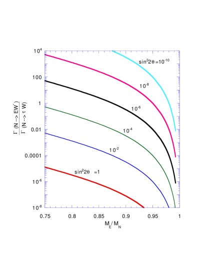
FIG. 9.: Relative branching ratios of the $N$ into $EW^{*}$ vs. $\tau W^{*}$ for various values of the mixing angle and the $E$ to $N$ mass ratio. One sees that the decay into $\tau W^{*}$ will dominate unless the mixing angle is very small. $\sin^{2}2\theta$ is the mixing between the third and fourth generations.

We see that the decay of $N$ into $\tau W^{*}$ tends to dominate, unless the mixing angle is extremely small. This leads to interesting phenomenology, as will be discussed in Section VII. If the $E$ is heavier than the $N$, the results are the same with $N\leftrightarrow E$ and $\nu_{\tau}\leftrightarrow\tau$.

Note that the decay rate of $E\rightarrow\nu_{\tau}W^{*}$ is proportional to $\sin^{2}\theta_{34}$. In the previous Section, we noted that this angle could be very small. Simplifying the expression for the decay, and assuming that the mass of the $E$ is greater than the $W$ (thus the $W$ is real), the width of the $E$ is given by

$$\Gamma(E\rightarrow\nu_{\tau}W)=(180\ {\rm MeV})\sin^{2}\theta_{34}\left({m_{E}\over m_{W}}\right)^{3}$$ (103)

Consider the four plausible values of $\sin^{2}\theta_{34}$ discussed in the previous Section. If $\sin^{2}\theta_{34}=m_{\tau}/m_{E}$, then the decay is very rapid and would occur at the vertex. If $\sin^{2}\theta_{34}=m_{\nu_{\tau}}/m_{N}$, then the lifetime is of the order of a few picoseconds, which has very interesting phenomenological consequences—it might be possible to see the charged track. If $\sin^{2}\theta_{34}=0$, then the $E$ is stable; this would be cosmologically disastrous, since they would bind with protons to form anomalously heavy hydrogen. If $\sin^{2}\theta_{34}=m_{W}^{2}/m_{Pl}^{2}$, then the lifetime is approximately $10-100$ years. We now address whether such a lifetime would pass cosmological muster.

The bounds on the lifetime of a fourth generation charged lepton were first discussed several years ago[177]. They considered charged lepton masses ranging from $50$ GeV to $50$ TeV. Stable leptons are ruled out by searches for heavy hydrogen. Since any decay of the $E$ will result in photon emission, failure to observe such emission in the diffuse photon background implies that the lifetime must be less than $10^{13}$ seconds (time of the cosmic background radiation (CMBR) production). Using COBE data on the CMBR, and requiring that the radiation in the decay not distort the CMBR, they found a bound on the lifetime which ranges from $10^{9}-10^{11}$ seconds as the mass ranges up to $1$ TeV. Very recently, an analysis by Holtmann, Kawasaki, Kohri and Moroi[178] looked at the radiative decay of a long-lived particle, $X$, and the effects on big-bang nucleosynthesis (the $E\rightarrow\nu_{\tau}W$ is not “radiative”, however, a significant fraction of the energy will eventually turn into photons, and the results are the same). The photons emitted in the decay may photodissociate deuterium (lowering its abundance) and helium (which raises the deuterium abundance), destroying the agreement between theory and observation. They give bounds on the lifetime as a function of $m_{X}Y_{X}$, where $Y_{X}\equiv n_{X}/n_{\gamma}$ is the relative abundance of the $X$. For heavy leptons, the abundance as a function of mass was calculated in Ref. [177]. For heavy lepton masses between $100$ and $500$ GeV, the contribution to $\Omega h^{2}$ varies from $0.05$ to $0.01$, leading to a value of $m_{X}Y_{X}$ which varies from $6\times 10^{-10}$ to $1.2\times 10^{-10}$ GeV (for a Hubble constant of $65$ km/sec/Mpc). From Tables 3-5 of Holtmann, Kawasaki, Kohri and Moroi[178], one can see that this correponds to an upper bound on the lifetime of between $10^{7}$ and $10^{8}$ seconds. Given the uncertainties in the abundance calculation, nucleosynthesis calculation, deuterium and helium abundance observations, etc., this is not inconsistent with a lifetime of $10-100$ years. Thus, the possibility that $\sin^{2}\theta_{34}=m_{W}^{2}/m_{Pl}^{2}$ is marginally allowed.

To summarize, if the mixing angle $\theta_{34}$ is not very small, then both the $N$ and $E$ will decay via Cabibbo-suppressed decays: $N\rightarrow\tau W^{*}$ and $E\rightarrow\nu_{\tau}W^{*}$. If the angle is very small (of the order of $m_{\nu_{\tau}}/m_{N}$ or less), then the heavier of the two will decay into the lighter, while the lighter decays via the Cabibbo-suppressed decay. In this case, the latter lifetime could be quite long, as long as a few picoseconds for $\sin^{2}\theta_{34}=m_{\nu_{\tau}}/m_{N}$ and as long as $10$ years for $\sin^{2}\theta_{34}=m_{W}^{2}/m_{Pl}^{2}$.

2 Nonchiral Leptons

As noted in the previous Sections, an interesting feature of models with a vector-like doublet (with small mixing with light generations) is that the two members of the doublet are degenerate in mass, at tree level. This degeneracy will be split by radiative corrections, and the size of this splitting is crucial in understanding the lifetimes and decay modes of the heavy leptons.

FIG. 10.: Diagrams contributing to the $E$-$N$ mass difference.

The splitting is due to the diagrams in Figure 10. The size of the splitting was first calculated by Dimopoulos, Tetradis, Esmailzadeh and Hall[179] (DTEH), and later calculated by Sher[180] (S) and even later by Thomas and Wells[181] (TW). The result is that the charged lepton is heavier than the neutrino, with a mass splitting of

$$\delta m={\alpha\over 2}m_{Z}f(m^{2}_{E}/m^{2}_{Z})$$ (104)

where

$$f(x)={\sqrt{x}\over\pi}\int_{0}^{1}dx\ (2-x)\ln\left(1+{x\over r(1-x)^{2}}\right).$$ (105)

For small $x$, $f(x)\rightarrow 0$, but for large $x$, $f(x)\rightarrow 1$, and thus the splitting reaches an asymptotic value of ${1\over 2}\alpha m_{Z}\simeq 350$ MeV for $m_{E}>>m_{Z}$. The splitting is plotted in Fig. 11.

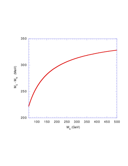
FIG. 11.: Mass difference between the $E$ and the $N$ as a function of the $E$ mass.

In DTEH[179], the authors considered very heavy leptons (of the order of several TeV) and looked at the question of whether such leptons could constitute the dark matter (they can’t). In S[180], the decay width of $E\rightarrow Ne\overline{\nu}$ and $E\rightarrow N\mu\overline{\nu}$ was calculated–the inverse of these widths corresponded to a lifetime of $1-2$ nanoseconds, which is obviously of great phenomenological interest. In S, it was also pointed out that the value of the splitting is very robust, and that supersymmetric contributions to the splitting turn out to be very small, since for most of parameter-space, the contributions turn out to be proportional to (${1\over 4}-\sin^{2}\theta_{W}$). In TW[181], it was pointed out that the dominant decay of the $E$ will be into $N\pi$ (a decay neglected in S), resulting in a much shorter (by roughly a factor of $10$) lifetime. The decay length then is of the order of centimeters, rather than tens of centimeters, greatly complicating detection. In Fig. 12, we plot the decay distance in the lab frame as a function of $m_{E}$ for a variety of center of mass energies. TW do propose an interesting signature involving triggering on an associated hard radiated photon; this will be discussed in Section VII.

Thus, in the vector-like doublet case, without significant mixing with the lighter generations, the charged member of the doublet is heavier and decays primarily into $N\pi$ (with a VERY soft pion) with a decay length given in Fig. 12.

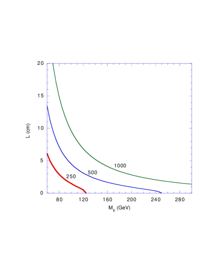
FIG. 12.: Decay length for the $E$ as a function of its mass. The lines are labelled with the center of mass energy of the collider in GeV.

The fully leptonic decays, even though they have branching ratios of only a few percent, might be easier to detect, although even in that case, the very soft electron or muon would be difficult to separate from backgrounds. If there is significant mixing, then both the $E$ and the $N$ will decay into the lighter generations. We now consider this possibility (which also applies to vector-like singlets).

We now consider the case in which there is significant mixing of vector-like leptons. By “significant”, we mean that the mixing angle, $\sin^{2}\theta_{34}$, is greater than about $10^{-11}$, so that the decay (see the expression for the lifetime above) occurs at the vertex. The results will be very similar to the chiral case, with one extremely important difference. Due to the breakdown of the GIM mechanism, the decays $E\rightarrow\tau Z$ and $N\rightarrow\nu_{\tau}Z$ will occur.

For $m_{E}>M_{Z}$, the branching ratios of the $E$ are given by[182]

$${\Gamma(E\rightarrow\tau Z)\over\Gamma(E\rightarrow\nu_{\tau}W)}={|U_{E\tau}|^{2}\over 2\cos^{2}\theta_{W}|U_{E\nu_{\tau}}|^{2}}{(m_{E}^{2}-2m^{2}_{Z}+m_{E}^{4}/m_{Z}^{2})(m_{E}^{2}-m_{Z}^{2})\over(m_{E}^{2}-2m^{2}_{W}+m_{E}^{4}/m_{W}^{2})(m_{E}^{2}-m_{W}^{2})}$$ (106)

There is no particular reason to believe that this branching ratio should be small. One might expect $|U_{E\nu_{\tau}}|^{2}$ to be of the order of $m_{\tau}/m_{E}$, as discussed in detail in the last Section. As discussed in the last Section, in the isosinglet heavy lepton case, one finds that $|U_{E\tau}|$ is of order of the ratio of $M_{34}$ to $M_{44}$ in the leptonic mass matrix which would be similar to $|U_{E\nu_{\tau}}|$; the resulting branching ratio would be very large. In the isodoublet heavy lepton case, there is an additional suppression of $m_{\tau}/m_{E}$, which results in a branching ratio of about $0.1\%$. Thus, one expects a branching ratio for $E\rightarrow\tau Z$ to be a fraction of a percent in the isodoublet case and very large in the isosinglet case.

It is important to note that even if the branching ratio is as low as a fraction of a percent, the background for a particle decaying into $\tau Z$ would be extremely small. A major problem with conventional heavy-lepton detection has been backgrounds; so the $E\rightarrow\tau Z$ signature, even with a branching ratio of a fraction of a percent or so, might very well be easiest to detect. This will be discussed in more detail in Section VII.

B Quarks

The discussion of the lifetime and decay modes of the quarks follows the general discussion of those of leptons, with a few crucial differences. While the $E$ and $N$ are certainly much heavier than the $\tau$, it is not necessarily the case that the $U$ and $D$ quarks are much heavier than the top. In addition, the mass splitting in the vector-like quark case is a factor of three smaller than that for vector-like leptons, which can drastically affect the decay modes and lifetime.

1 Chiral Quarks

Due to constraints from the $\rho$ parameter, the $U$ and $D$ quarks cannot have masses which are too different, and thus the decay $U\rightarrow D+W$ or $D\rightarrow U+W$ cannot occur into real $W$’s. Suppose, for the moment, that $m_{U}>m_{D}$. Then the allowed decays of the $U$ will be $U\rightarrow(D\ {\rm or}\ q)+W^{*}$, $U\rightarrow q+W$, where $W^{*}$ refers to a virtual $W$. The allowed decays of the $D$ are $D\rightarrow(t\ {\rm or}\ q)+(W^{*}\ {\rm or}\ W)$. In addition, one can have a flavor-changing neutral current decay $D\rightarrow b+Z$, which (in the chiral case) can occur through one loop. The fact that the flavor-changing neutral decay of a fourth generation quark could be significant was first pointed out by Barger, Phillips and Soni[183], and followed up by Hou and Stuart[184, 185]. In the latter works, they noted that the decay $D\rightarrow b+Z$ dominates over other flavor-changing decays, such as $D\rightarrow b+\gamma$ and $D\rightarrow b+g$. The possible $D\rightarrow b+Z$ mode, like the $E\rightarrow\tau+Z$ mode, is very important phenomenologically due to the very clear signatures[186, 187]. Precise analytical formulae for the various decays, and a discussion of the decays of the $D$ (from which much of the discussion below is taken), can be found in the recent work of Frampton and Hung[188].

The two-body and three-body decay widths are given by the first of Eq. 99, with the obvious substitutions of $|V_{Dq}|$ or $|V_{Uq}|$ for $\cos^{2}\theta_{34}$. The flavor-changing neutral current decay is given by

$$\Gamma(D\rightarrow bZ)=|V_{Dt}|^{2}{G_{F}(m_{D})^{3}\over 4\pi\sqrt{2}\cos^{2}\theta_{W}}\left(({g^{2}\over 16\pi^{2}})^{2}\Delta(m_{U},m_{t})\right)I_{2}(m_{b}/m_{D},m_{Z}/m_{D})$$ (107)

where we have assumed, for simplicity, that $V_{Ub}=-V_{Dt}$ so there will be a GIM suppression when $m_{U}=m_{t}$ (this occurs in most models). We have also assumed that $V_{UD}$ is approximately unity. Here,

$$\Delta(m_{U},m_{t})=\left({M_{U}^{2}-m_{t}^{2}\over m^{2}_{W}}(\ln({m_{W}^{2}\over m^{2}_{heavy}})-1)\right)^{2}$$ (108)

and $m_{heavy}$ refers to the heavier of $U$ and $t$. The factor $I_{2}$ is the standard two-body phase space factor, which is unity in the limit $m_{D}>>m_{Z}$.

The $U$ decays very rapidly, at the vertex (unless the masses are unusually close together, which is unlikely in the chiral quark case, since they arise from different terms); however the $D$ can be long-lived. The decay modes of the $D$ depend crucially on the mass.

First, suppose the $D$ is lighter than the top quark. The decay can only occur into $c+W$ or $b+Z$ (one expects the decay into $u+W$ to be highly suppressed). Two important issues arise: which of these has a larger branching ratio (since their phenomenological signatures are very different), and is it possible that the decay length might be large enough to be detected? We now address both of these questions.

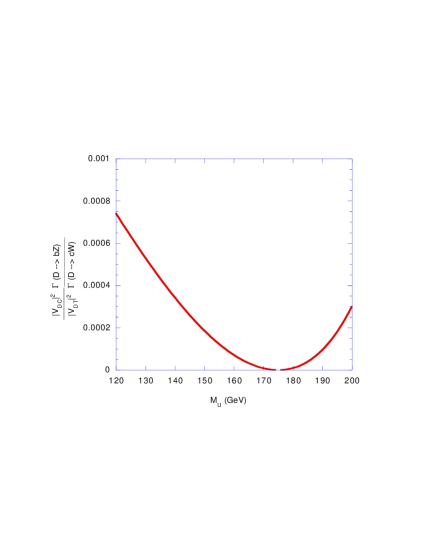
FIG. 13.: Ratio of width of $D\rightarrow b+Z$ to that of $D\rightarrow c+W$. Note the GIM suppression of the FCNC decay when the $U$ mass equals the top mass.

From the above formulae, the ratio of the widths can be calculated. The only dependence of the D-mass in this ratio is in the ratio of phase spaces–unless the $D$ is fairly close in mass to the $Z$ this ratio is near unity. The only mass-dependence is then in the $U$ mass-dependence in $\Delta(m_{U},m_{t})$ above. The result is given in Figure 13, for various values of the $U$ mass (recall the fact that the $U$ and $D$, in this range, cannot be different in mass by more than $20$ GeV due to $\rho$ parameter constraints). The results depend on the ratio of $|V_{Dc}|$ to $|V_{Dt}|$. Since the former is “doubly-Cabbibo-suppressed” (crossing two generations), one expects the ratio to be small. We see that the $D\rightarrow bZ$ decay mode dominates if the ratio is small, whereas $D\rightarrow cW$ dominates if it is large (unless the $U$ mass is very near the top mass. Since there is little theoretical guidance as to the size of this ratio, both signatures should be looked for.

Could a vertex be seen? From the expression for $\Gamma(D\rightarrow bZ)$, one can see that the width of this mode[184] is between $10^{-4}|V_{Dt}|^{2}$ MeV and $10^{-2}|V_{Dt}|^{2}$ MeV over the mass range of interest. This implies that the lifetime will be at most $6\times 10^{-18}/|V_{Dt}|^{2}$ seconds. This would mean that one must have $|V_{Dt}|<<10^{-3}$ in order to detect a vertex. Although such a small angle is not expected in the chiral sequential quark case (the Aspon Model involves non-chiral quarks), it is not excluded, if one has a flavor symmetry with an almost unbroken $3+1$ structure.

For $m_{D}$ between $177$ and $256$ GeV, the $D$ can decay into the top quark via the three-body decay into a virtual $W$. In this case, $D\rightarrow t+W^{*}$ will be competetive with $D\rightarrow c+W$ and $D\rightarrow b+Z$—the latter are suppressed by the doubly-Cabibbo suppressed mixing angle or the extra loop, the former is suppressed by three body phase space. If we compare the rate for $D\rightarrow t+W^{*}$ with $D\rightarrow b+Z$, the mixing angle cancels out. In Figure 14, we have plotted the ratio of these two decays.

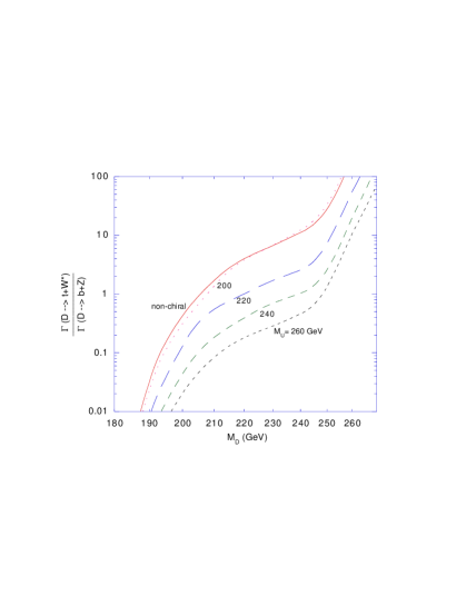
FIG. 14.: Ratio of width of $D\rightarrow t+W^{*}$ to that of $D\rightarrow b+Z$ for various values of $M_{U}$. The non-chiral line corresponds to the vectorlike doublet case, which is independent of $M_{U}$. For the non-chiral isosinglet case, the ratio is too small to be seen on the graph.

Thus, as pointed out in Ref. [188], the three-body decay of the $D$ is irrelevant for $D$ masses below about $230$ GeV (depending on $M_{U}$), and thus the arguments of the previous two paragraphs are unchanged.

As the mass increases beyond $230$ GeV, the three body decay becomes more important, and as soon as the mass exceeds $256$ GeV, the two-body decay $D\rightarrow t+W$ becomes accessible. At that point, $D\rightarrow t+W$ becomes the dominant decay. Again, very small mixing would be needed to see the vertex, $|V_{Dt}|<10^{-5}$.

What about the decay of the $U$ quark (again, assuming that $m_{U}>m_{D}$)? The U can decay into $D$ and a virtual $W$, $U\rightarrow D+W^{*}$, or into a light quark (most likely a $b$) and a real W, $U\rightarrow b+W$. Which decay mode dominates depends on how close the $U$ and $D$ are in mass and on the $|V_{Ub}|$ mixing angle. This was discussed in Ref. [188]. As $m_{U}$ varies from $180$ to $250$ GeV, the width for $U\rightarrow b+W$ varies from $1.75|V_{Ub}|^{2}$ GeV to $4.7|V_{Ub}|^{2}$ GeV. For $U\rightarrow D+W^{*}$, the width (assuming $|V_{UD}|$ is nearly unity) is $5.2\times 10^{-5}$ GeV for $m_{U}/m_{D}=1.1$, and drops to $3\times 10^{-8}$ GeV for $m_{U}/m_{D}=1.02$. For moderate mixing angles, $|V_{Ub}|>0.003$, the $U\rightarrow b+W$ decay mode will always dominate. For mixing angles in the range between $10^{-3}$ and $10^{-4}$, which dominates dependes sensitively on the mass ratio between the $U$ and the $D$. For mixing angles below $10^{-4}$, the $U\rightarrow D+W^{*}$ will dominate. In no cases will the width be small enough so that a vertex can be seen: the $U$ will decay at the vertex.

If $m_{D}>m_{U}$, everything we have said above will carry through, exchanging $t$ with $b$, etc. A principal difference is that one can consider lighter long-lived $U$ quarks (since one can have $m_{U}<m_{t}$) than for $D$ quarks.

To summarize, if $m_{U}>m_{D}$, then the primary decays modes of the $D$ will be $D\rightarrow c+W$ and $D\rightarrow b+Z$ if the $D$ mass is below about $230$ GeV. The former will dominate if $|V_{cD}|/|V_{Dt}|$ is greater than $0.01$, the latter will dominate if it is less than $0.001$. As the $D$ mass increases above $230$ GeV, the decay $D\rightarrow t+W^{*}$ begins to dominate. In all cases, one must have very small mixing angles ($|V_{Dt}|<10^{-3}$ or $10^{-5}$, depending on the mode) in order for the decay to occur a measureable distance from the vertex. The $U$ will always decay at the vertex, into either $D+W^{*}$ or $b+W$, depending on the precise masses and mixing angles.

2 Nonchiral Quarks

For vector-like quarks, either isosinglet or isodoublet, many of the above results are unchanged. As noted in Ref. [188], the decay widths into real or virtual $W$’s will not be significantly changed. As in the nonchiral lepton case, there are two major differences: the mass difference between the $U$ and the $D$ in the isodoublet case is calculable (if mixing is small), and the flavor-changing neutral decay $D\rightarrow bZ$ can occur at tree level.

In the isodoublet case, the mass difference between the $U$ and the $D$ can be shown[180] to be $1/3$ that of the lepton case, and will thus be between $70$ and $110$ MeV, if the mixing with lighter generations is small. This means that the hadronic decay is forbidden, and the only decay would be $U\rightarrow De\nu$, with a lifetime of the order of microseconds. Thus, in the absence of mixing, both the $U$ and the $D$ would be absolutely stable, as far as accelerators are concerned, and the mass difference is irrelevant. We thus must consider both $U$ and $D$ decays.

The $D$ can decay, as in the chiral case, into either $c+W$, $t+W^{*}$, $t+W$ or $b+Z$. The only difference in the above discussion is the rate for $D\rightarrow b+Z$. In the expression for $\Gamma(D\rightarrow b+Z)$ in the last section, one must replace the factor of $g^{4}\Delta(m_{U},m_{t})/64\pi^{4}$ from the loop with $m_{b}^{2}/m_{D}^{2}$, in the isodoublet case, and with unity in the isosinglet case (the factor of $|V_{Dt}|^{2}$ is the same in each case). In the isodoublet case, this does not change the result for the width by more than an order of magnitude, but in the isosinglet case, it increases the width by roughly three orders of magnitude.

First, if the $D$ is lighter than the top quark, then the decay modes in the isodoublet case are very similar to the chiral case—the results depend sensitively on the ratio of $|V_{Dc}$ to $|V_{Dt}|$, and either the $D\rightarrow c+W$ and $D\rightarrow b+Z$ will be dominant. A displaced vertex can only be seen if $|V_{Dt}|<10^{-3}$. This is expected in the Aspon Model case, and thus one can expect a significantly displaced vertex in the model (as emphasized in Ref. [188]). In the isosinglet case, the absence of the $m_{b}^{2}/m_{D}^{2}$ suppression makes the $D\rightarrow b+Z$ mode dominant, and also requires that $|V_{Dt}|<<10^{-5}$ in order for a displaced vertex to be seen (which is not expected in the Aspon Model).

If the $D$ is heavier than the top quark, then the argument in the previous section carries through without significant modification in the isodoublet case; the cross-over where the three body decay becomes relevant is closer to $210$ GeV than to $230$ GeV. In the isosinglet case, however, the $D\rightarrow b+Z$ mode dominates, even over the two-body top quark decay, until $m_{D}$ is well over $300$ GeV, and remains significant even to much higher masses.

Thus, we see that in either the chiral or non-chiral case, the decay $D\rightarrow b+Z$ is very important. It was pointed out in Ref. [188] that, if this mode were detected, then one could look at the chirality of the $Z$ to determine which of the two cases applies. This might be the quickest way to determine the chirality of the heavy quarks.

Unless the $U$ is very heavy, above $310$ GeV, the flavor-changing neutral decay $U\rightarrow t+Z$ is forbidden or highly suppressed by phase space. Since $U\rightarrow c+Z$ is suppressed by small mixing angles, one has the $U\rightarrow b+W$ decay mode dominating. Again, one can only detect the vertex if the angle is very small, less than $10^{-5}$.

V Dynamical Symmetry Breaking

It is fair to say that perhaps one of the most important discoveries that can be made in the future will be that of the Higgs boson. In the absence of any alternative plausible explanation for particle masses, the concept of spontaneous breakdown of a gauge symmetry via the Higgs field as the origin of all masses is universally accepted. The only problem is that it has not been found. Not only does one not know its mass, but one also does not know in what shape or form it should be. One fact that we do know however , regardless of how massive and in what form the Higgs boson may be, is the scale of electroweak symmetry breaking: $v=246$ GeV. All masses in the SM are expressed in terms of that scale, e.g. $M_{W}=(1/2)gv$ and $m_{i}=g_{Y_{i}}v/\sqrt{2}$, where $g_{Y_{i}}$ are Yukawa couplings. There is a rather intriguing fact: With $v/\sqrt{2}\sim 174$ GeV, it follows that the top quark Yukawa coupling, $g_{t}$, is of order unity, unlike all other fermions. That the top quark is so heavy and its mass is so close to the electroweak breaking scale is cause to wonder about any relationship that it might have with the mechanism of symmetry breaking itself.

If the top quark mass is so close to the electroweak scale, is it possible that it itself is reponsible for the breaking of the electroweak symmetry? This fascinating possibility was first entertained by Refs.[43]-[46]. It is now commonly refered to as “top-condensate models”. In these models, the Higgs boson is generally viewed as a $t\bar{t}$ composite field generated by some unknown dynamics at a scale $\Lambda\gg 246$ GeV. In other words, the electroweak symmetry breaking is dynamical in these scenarios, i.e. it is broken by a $t\bar{t}$ condensate or something similar. One interesting feature of these models is the prediction of a heavy fermion mass (e.g. the top quark mass or a fourth generation mass) as a function of the Higgs boson mass through the so-called compositeness conditions. Before describing these models and their variants, let us first summarize the results of the simplest version, that of Bardeen, Hill and Lindner [46]. In Ref. [46], the first scenario including only a heavy top quark predicted a top mass of order 230 GeV. This is now excluded. Ref. [46] also presented results involving a heavy, degenerate fourth generation quark doublet, assuming that the top quark and other fermions are much lighter. This result combined with the known top quark mass indicates that something else other than the top quark alone must exist if this picture has any chance of being correct.

The subject of dynamical symmetry breaking à la top-condensate deserves a whole review; a book on the topic already exists [189]. The best we could do here is to review salient points and results, especially those pertaining to the subject of this review. We first state the so-called compositeness conditions used in the top-condensate type of models. As we shall see below, these conditions allow us to relate the masses of the heavy fermions to that of the Higgs boson. Simply speaking, it is the requirement that the Higgs quartic coupling $\lambda$ and the relevant Yukawa couplings diverge at the same scale $\Lambda_{C}$ (the Landau poles) while the ratio of $\lambda$ to the square of the Yukawa coupling(s) remains finite, namely

$$\lambda(\mu),~{}g_{t}(\mu)\stackrel{{\scriptstyle\mu\to\Lambda_{C}}}{{\longrightarrow}}\infty$$ (109)

$$\lambda(\mu)/g^{2}_{t}(\mu)\stackrel{{\scriptstyle\mu\to\Lambda_{C}}}{{\longrightarrow}}\mbox{const.}$$ (110)

where $g_{t}$ can be either the top or just a generic Yukawa coupling. The above boundary conditions modify the structure of the SM Lagrangian at the scale $\Lambda_{C}$ in the following way. Let us consider a simple toy model where there is a degenerate heavy quark doublet $Q=(U,D)$ coupled to the Higgs field $\Phi$ (light fermions will be ignored in this discussion). Let us rescale $\Phi$ as follows

$$\Phi\longrightarrow\Phi_{0}/g_{f},$$ (111)

where $g_{f}$ is the Yukawa coupling of the degenerate quark doublet. The SM Lagrangian (with only that degenerate doublet present) becomes

$${\cal L}={\cal L}_{kinetic}(U,D)+Z_{\Phi}D_{\mu}\Phi^{\dagger}_{0}D^{\mu}\Phi_{0}+{\widetilde{m}}^{2}\Phi^{\dagger}_{0}\Phi_{0}-\frac{\widetilde{\lambda}}{4}(\Phi^{\dagger}_{0}\Phi_{0})^{2}+{\bar{Q}}_{L}\Phi_{0}D_{R}+{\bar{Q}}_{L}{\Phi^{C}_{0}}U_{R}+\mbox{h.c.},$$ (112)

where

$$\Phi^{C}_{0}=i\sigma_{2}\Phi_{0}^{\ast},\qquad Z_{\Phi}=1/g^{2}_{f},\qquad\widetilde{m}^{2}=Z_{\Phi}m^{2},\qquad\mbox{and}\qquad\widetilde{\lambda}=Z_{\Phi}^{2}\lambda.$$ (113)

The first remark one can make when one looks at the above expressions is the compositeness condition itself: the vanishing of the wave function renormalization constant. Indeed, as can be seen from the expression for $Z_{\Phi}$, one immediately notices that, if $g_{f}$ has a Landau singularity at some scale $\Lambda_{C}$, the wave function renormalization constant for the Higgs field, $Z_{|Phi}$, vanishes at that same scale. In other words, the Landau pole is identified with the compositeness scale. Furthermore, if $\lambda$ and $g_{f}$ develop a singularity at the same scale in such a way that conditions  (109) are satisfied, the Lagrangian at the compositeness scale becomes

$${\cal L}={\cal L}_{kinetic}(U,D)+{\bar{Q}}_{L}\Phi_{0}D_{R}+{\bar{Q}}_{L}\Phi^{C}_{0}U_{R}+{\widetilde{m}}^{2}\Phi^{\dagger}_{0}\Phi_{0}+\mbox{h.c.}$$ (114)

$\Phi_{0}$ is now just an auxiliary field and can be integrated out, resulting in a Nambu-Jona-Lasinio form for the Lagrangian, namely

$${\cal L}={\cal L}_{kinetic}(U,D)+G_{0}{\bar{Q}}_{L}(U_{R}{\bar{U}}_{R}+D_{R}{\bar{D}}_{R})Q_{L},$$ (115)

where $G_{0}=-1/\widetilde{m}^{2}.$ In this picture, the Higgs boson becomes a fermion-antifermion composite particle below the scale $\Lambda_{C}$.

What might be even more interesting is the relationship between the Higgs boson mass and that of the heavy fermions in the top-condensate type of scenario. In particular, the Higgs mass, $m_{H}$, can be seen to be bounded from above by $2m_{f}$ and from below by $m_{f}$, where $m_{f}$ is a heavy fermion mass. The search for a heavy fermion is intimately tied to the search for the Higgs boson-a feature already seen in the discussion of gauge coupling unification [65]. To see this in the context of the top-condensate type of model, let us look at the RG equations for $\lambda$ and $g_{f}$, the heavy fermion Yukawa coupling, at one loop level (the one-loop terms of Eq.  (77)) in the toy model with one doublet of heavy quarks. Let us define $x=\lambda/g_{f}^{2}$. The one-loop RG for $x$ is then

$$16\pi^{2}\frac{dx}{dt}=24g^{2}_{f}(x-x_{+})(x-x_{-}),$$ (116)

where $x_{\pm}=(-1\pm 3)/4$, if both members of the quark doublet are degenerate in mass, or $x_{\pm}=\frac{1}{16}(-1\pm\sqrt{65})$, if one member is much heavier than the other one (e.g. the 3rd generation case). The boundary conditions  (109) are satisfied if $x$ is one of the two fixed points, $x_{\pm}$. The solution $x_{-}$ (always negative) is ruled out by vacuum stability. This leaves us with $x_{+}$. From the definition of $m_{f}$ and $m_{H}$, one can then obtain a relationship between these two masses as follows:

$$m_{H}^{2}=4m_{f}^{2}\,x_{+}.$$ (117)

In the large $N_{c}$ limit, the right hand side of Eq.  (116) becomes $4N_{c}(x-1)$ with the fixed point being $x=1$ which implies $m_{H}=2m_{f}$, a familiar result found in the Nambu-Jona-Lasinio model. Since $x_{+}$ is always greater than 1/4, one can easily see that, for finite $N_{c}$, one obtains the bound

$$m_{f}<m_{H}<2m_{f}.$$ (118)

As we have mentioned above, a necessary condition for this scenario to work is the boundary  (109). The minimal SM with three generations unfortunately does not satisfy these boundary conditions: the top quark with a mass of 175 GeV is simply too “light”. One needs eiher a heavier quark (216-230 GeV), which cannot be the case with the minimal SM, or more heavy quarks or leptons such as in the four generation scenario. The four generation case was studied by Hill, Luty and Paschos [190] in the context of Majorana neutrinos. Later, Hung and Isidori [117] also examined the four generation scenario as part of an overall “anatomy” of the Higgs mass spectrum, starting form $m_{H}$ of 65 GeV to $m_{H}\geq 2m_{Z}$. It was in this last mass range, $m_{H}\geq 2m_{Z}$, that the focus on top-condensate types of models was diverted to. In their analysis, Ref. [117] assume a Dirac mass for the fourth neutrino and degenerate quarks and degenerate leptons for the fourth generation. It turns out that the inclusion of such a fourth generation drastically modifies the evolution of the couplings even if these fermions were lighter than the top quark. In the analysis of Ref. [117], Eqs.  (77) were used at the one loop level. The results are shown in Fig.15 below, where the mass of the top quark is fixed at 175 GeV and that of the fourth lepton doublet is fixed at 90 GeV.

FIG. 15.: RG evolution of the Yukawa couplings $g^{2}_{t}$ (full and dash-dotted lines) and $g^{2}_{q}$ (dashed lines). The top mass is always fixed to be 175 GeV and the heavy-lepton mass is assumed to be 90 GeV. The dash-dotted line is the evolution of $g^{2}_{t}$ without extra fermions. Near each dashed line is indicated the value of $m_{q}$ and the corresponding value of $m_{H}$ obtained by the requirement $\Lambda_{L}=\Lambda_{q}$ (the error on both $m_{H}$ and $m_{q}$ is about $\pm 10$ GeV.

A few remarks are in order concerning the above figure. As the figure caption already indicates, the dash-dotted line represents the top Yukawa coupling squared, $g_{t}^{2}$, as a function of energy for the minimal SM. One can see that $g_{t}^{2}$ actually decreases in value with energy and remains finite at the Planck scale. This is so because a mass of 175 GeV is “too small” to provide a large enough initial value plus the fact that the contribution from the QCD coupling to the $\beta$ function for $g_{t}^{2}$ occurs with the opposite sign. When a fourth generation is added, the evolution of the couplings change drastically, partly due to the fact that there are more degrees of freedom than the minimal case. So, as long as the initial Yukawa couplings of the fourth generation are not too small, there will be Landau poles that appear below the Planck scale. As one can see from Fig.15, this occurs when the fourth generation quark mass $m_{Q}\gtrsim 150$ GeV. Also an interesting phenomenon occurs: all Yukawa couplings “drag” each other in such a way that they all “blow up” at the same point. The top quark Yukawa coupling, which by itself decreases with energy, is now “dragged” in such a way as to develop a Landau pole at the same time as the fourth generation quarks. These results- the existence of Landau poles below the Planck scale in the presence of a fourth generation- encourage a reconsideration of the top-condensate type of model.

Since the quartic coupling $\lambda$ is a free parameter, one can now choose its initial value, i.e. its mass, in such a way that the boundary conditions  (109) are satisfied. This procedure results in a relationship between the fourth generation quark mass and the Higgs mass. This is shown in Fig. 15 ($m_{f}$ is the notation used in the figure to refer to the fourth generation quark mass instead of $m_{Q}$ which is used here). The relationship for low 4th generation quark mass (e.g. 150 GeV) is strikingly similar to the one obtained in the discussion of the gauge coupling unification of Ref. [65]. The range of mass used in Ref. [117] for $m_{Q}$ is however considerably larger than that of Ref. [65] because, in that study of a top-condensate type of model, no constraint on where the Landau poles should be has been used. In fact, for masses larger than 150 GeV, the Landau poles move down in energy. For example, if $m_{Q}=230$ GeV which corresponds to $m_{H}=300$ GeV, the Landau pole is situated at approximately 100 TeV. As remarked by Ref. [117], the relationship between the Higgs mass and the fourth generation quark mass approaches more and more the fixed point value for a degenerate quark doublet, $m_{H}=\sqrt{2}m_{Q}$, as the Landau pole “approaches” the electroweak scale. This can be seen in the figure shown above.

The scenario described above intimately links the search for the fourth generation quarks and leptons to that of the Higgs boson, and vice versa. It is not clear at this point how the higher mass values ($>160$ GeV) for the fourth generation quarks would affect the evolution of the gauge couplings, except for the fact that perturbation theory breaks down above the Landau poles and it is not legitimate to evolve those couplings beyond that point. For the purpose of this report, we shall however leave open the possibility of such top-quark condensate type of models as a possible mechanism for electroweak breaking. It is partly for this reason that the range of masses considered in the search for long lived quarks by Frampton and Hung [188] is larger than the mass range used in the study of gauge coupling unification of Hung [65].

Recently [191], there was an analysis of the two-loop RG equations in the SM with three and four generations. Although many results presented there [191] were already discussed in [65] and [117], there were statements that are not correct. In order to clarify the issues, we repeat the statements of Ref. [191] and explain why they are misleading. Ref. [191] chose the masses of the leptons and the quarks of the fourth generation as follows: $m_{L}/m_{Q}=1/2$ and 1, and restricted $m_{Q}$ to be greater than 180 GeV which was referred to by the authors as the direct experimental constraint. Furthermore, an upper bound of 200 GeV for $m_{H}$ was used. Using these constraints, Ref. [191] claimed that a fourth generation is ruled out by plotting the allowed regions in the $m_{H}-m_{Q}$ plane (Fig. 11 of [191]). First, $m_{Q}$ less than 180 GeV is not ruled out by direct experiment if a long-lived quark decays in the detector at a distance between 100 $\mu$m and 1 m, a subject discussed by Frampton and Hung [188]. As we shall discuss in the section on experiments, there is and will be such a search at the Tevatron. Second, the constraints on $m_{H}$ at the present time from precision experiments are rather loose at best. A much larger bound than 200 GeV is possible [192]. For example Refs. [193, 194, 195] gave an upper bound as high as $\sim$ 280 GeV, while Ref. [196] gave an upper bound (within 95 % CL) from 340 GeV to 1 TeV. In summary, the mass ranges used by [191] to rule out a fourth generation are not warranted. In fact, the values used by Hung [65], $m_{Q}=151$ GeV and $m_{H}=188$ GeV, were shown to lead to a better unification of the SM gauge couplings, and higher masses (such as 180 GeV) for $m_{Q}$ were not used because precisely of the fact that the Landau poles were much too low to trust perturbation theory in the evolution of the gauge couplings.

As the above discussion and earlier ones made it crystal clear, there are several theoretical reasons for looking at quarks and leptons beyond the third generation. In particular, our primary motivation in this review is to examine those reasons which “predict” fermion masses which are within reach either of present experiments such as the ones performed at the Tevatron or at future machines such as the LHC, NLC, etc. By “within reach”, we mean masses which are close to the top quark mass ( $\sim$ 150 -230 GeV) for the quarks. It goes without saying that there exists also plenty of reasons for considering fermions which are much heavier than the top quark, some of which are even primary focus of the topics discussed in this section: the techniquarks and leptons of Technicolor models [197, 198, 199, 200]. It is outside of our goal to review such topics but for completeness, we shall give a brief description of one of such scenarios: the topcolor assisted Technicolor model.

Our discussion of top-condensate type of models above relies on one crucial assumption: The entire electroweak symmetry breaking is due to the condensate of the top quark and/or that of the fourth generation quark. The topcolor assisted Technicolor model of Hill [201] did away with that assumption. But then how does one explain the fact that the top quark mass is so much larger than all other fermion masses and so close to the electroweak breaking scale? The salient points of the topcolor model are basically the assumptions that the electroweak symmetry is still broken by some form of Technicolor, there exists an extra (“topcolor”) group, $SU(3)_{1}\otimes U(1)_{Y_{1}}$, which couples preferentially to the third family and which triggers a dynamical condensate for the top quark, giving rise to a large top mass. This new “topcolor” group is assumed to be spontaneously broken by Technicolor at a scale $\sim$ 1 TeV. An extended Technicolor interaction (ETC) is also assumed so that quarks and leptons can obtain some mass which is much smaller than the top mass. The top quark itself obtains most of its mass from the condensate with a small contribution coming from ETC. Variations of the model include cases in which there are $SU(2)$ singlet quarks which are however very massive ($\sim$ 1 TeV). In any case, all fermions beyond the 3rd generation is these models have masses around 1 TeV. Although there is a rich phenomenology involving objects such as top-pions, etc., it is beyond the scope of this review to discuss it here.

We end this section by mentioning that there are interesting recent developments on the subject of electroweak symmetry breaking involving the so-called seesaw mechanism of quark condensation [202, 203]. This is yet another variant of the topcolor model. In this particular scheme, the top quark mass obtains its “observed” value dynamically by a mass mixing with a new SU(2) singlet quark $\chi$ of the form $\mu_{\chi t}\bar{\chi}_{L}t_{R}+m_{t\chi}\bar{t}_{L}\chi_{R}+\mu_{\chi\chi}\bar{\chi}_{L}\chi_{R}$ with $m_{t\chi}\sim 0.6$ TeV, $\mu_{\chi t}\sim 0.9$ TeV and $\mu_{\chi\chi}\sim 2$ TeV. The physical top mass is found by diagonalizing that $2\times 2$ matrix giving $m_{t}\approx\mu_{\chi t}m_{t\chi}/\mu_{\chi\chi}$. The other mass eigenstate would be $\sim 2$ TeV and it might not be easy to be observed directly. The model predicts a number of pseudo Nambu-Goldstone bosons, some of which are $\chi$- bound states. How this new degree of freedom manifest itself experimentally is a subject which is under active investigation.

One last comment which is worth mentioning here is the mass of the Higgs boson in the different variants of the topcolor model. Generically, the physical Higgs scalar would have a mass of the order of a TeV just like standard Technicolor models. However, in the seesaw version of the topcolor model, there appears an extra “light” Higgs scalar (in addition to the charged ones) as one would have in a two-Higgs doublet model. Depending on a delicate cancellation of some parameters of the model, one could have a “truly light” scalar with mass of O(100) GeV. These remarks are meant to emphasize the importance of the search of Higgs scalar(s) in addition to that of new quarks and leptons.

VI CP Violation.

A CP Violation in the Standard Model.

At first sight, there may appear to be no connection between additional quarks and leptons and the violation of CP symmetry. The object of this subsection is therefore to convince the reader that the better understanding of CP violation may necessitate the incorporation of additional fermions. This is not an inevitable conclusion but it is a suggestive one.

To set the scene, we need to describe the status of CP symmetry and its violation in the context of the unadorned standard model. This discussion will be in two separate parts: weak CP violation (the KM mechanism), and the strong CP problem. The former is not really a problem for the standard model, merely one that is not yet verified unambiguously by experiment. The latter, the strong CP problem, is definitely a difficulty, a shortcoming, for the standard model and one whose solution (we shall mention the axion possibility) is still unknown.

The gauge group of the standard model is $SU(3)_{C}\times SU(2)_{L}\times U(1)_{Y}$, broken at the weak scale to $SU(3)_{C}\times U(1)_{Y}$. Under the standard group the first generation transforms as:

$$Q_{L}=\left(\begin{array}[]{c}u\\ d\end{array}\right)_{L},\bar{u}_{L},\bar{d}_{L};\hskip 14.45377ptL_{L}=\left(\begin{array}[]{c}\nu_{e}\\ e^{-}\end{array}\right)_{L},e^{+}_{L}$$ (119)

and the second ($c,s,\nu_{\mu},\mu$) and third ($t,b,\nu_{\tau},\tau$) generations are assigned similarly.

The quarks acquire mass from the vacuum expectation value (VEV) of a complex $SU(2)_{L}$ doublet of scalars $\phi=\left(\begin{array}[]{c}\phi^{+}\\ \phi^{0}\end{array}\right)$ giving rise to up and down quark mass matrices:

$$M(U)=\lambda_{ij}^{U}<\phi^{0}>;M(D)=\lambda_{ij}^{D}<\phi^{0}>$$ (120)

which are arbitrary matrices that may, without loss of generality, be chosen to be hermitian. The matrices $M(U),M(D)$ of Eq. (120) are defined so that the Yukawa terms give e.g. $Q_{L}M(U)u_{R}+h.c.$ and can be diagonalized by a bi-unitary transformation:

$$K(U)_{L}M(U)K(U)_{R}^{-1}=diag(m_{u},m_{c},m_{t})$$ (121)

$$K(D)_{L}M(D)K(D)_{R}^{-1}=diag(m_{d},m_{s},m_{b})$$ (122)

These mass eigenstates do not coincide with the gauge eigenstates of Eq.(119) and hence the charged $W$ couple to the left-handed mass eigenstates through the $3\times 3$ CKM matrix $V_{CKM}$ defined by:

$$V_{CKM}=K(U)_{L}K(D)_{L}^{-1}$$ (123)

This is a $3\times 3$ unitary matrix which would in general have 9 real parameters. However, the five relative phases of the 6 quark flavors can be removed to leave just 4 parameters comprising 3 mixing angles and a phase. This KM phase underlies the KM mechanism of CP violation.

With N generations and hence a $N\times N$ mixing matrix there are $N(N-1)/2$ mixing angles and $(N-1)^{2}$ parameters in the generalized CKM matrix. The number of CP violating phases is therefore $(N-1)^{2}-N(N-1)/2=(N-1)(N-2)/2$. This is zero for $N=2$, one for $N=3$, three for $N=4$, and so on. In particular, as Kobayashi and Maskawa [27] pointed out, with three generations there is automatically this source of CP violation arising from the $3\times 3$ mixing matrix. This is the most conservative approach to CP violation. This source of CP violation is necessarily present in the standard model; the only question is whether it is the only source of CP violation. Since the only observation of CP violation remains in the neutral kaon system, there is not yet sufficient experimental data to answer this question definitively.

There are various equivalent ways of parametrizing the CKM matrix. That proposed[27] by KM involved writing:

$$V_{CKM}=\left(\begin{array}[]{ccc}cos\theta_{1}&-sin\theta_{1}cos\theta_{3}&-sin\theta_{1}sin\theta_{3}\\ sin\theta_{1}cos\theta_{2}&cos\theta_{1}cos\theta_{2}cos\theta_{3}-sin\theta_{2}sin\theta_{3}e^{i\delta}&cos\theta_{1}cos\theta_{2}sin\theta_{3}+sin\theta_{2}cos\theta_{3}e^{i\delta}\\ sin\theta_{1}sin\theta_{2}&cos\theta_{1}sin\theta_{2}cos\theta_{3}+cos\theta_{2}sin\theta_{3}e^{i\delta}&cos\theta_{1}sin\theta_{2}sin\theta_{3}-cos\theta_{2}cos\theta_{3}e^{i\delta}\\ \end{array}\right)$$ (124)

Another useful parametrization[204] writes:

$$V_{CKM}=\left(\begin{array}[]{ccc}1-\frac{1}{2}\lambda^{2}&\lambda&\lambda^{3}A(\rho-i\eta)\\ -\lambda&1-\frac{1}{2}\lambda^{2}&\lambda^{2}A\\ \lambda^{3}A(1-\rho-\eta)&-\lambda^{2}A&1\\ \end{array}\right)$$ (125)

In Eq.(125), $\lambda$ is the sine of the Cabibbo angle $sin\theta_{1}$ in Eq.(124) and CP violation is proportional to $\eta$. If we write the CKM matrix a third time as:

$$V_{CKM}=\left(\begin{array}[]{ccc}V_{ud}&V_{us}&V_{ub}\\ V_{cd}&V_{cs}&V_{cb}\\ V_{td}&V_{ts}&V_{tb}\\ \end{array}\right)$$ (126)

then the unitarity equation $(V_{CKM})^{\dagger}V_{CKM}=1$ dictates, for example, that

$$V_{ub}^{*}V_{ud}+V_{cb}^{*}V_{cd}+V_{tb}^{*}V_{td}=0$$ (127)

This relation is conveniently represented as the addition of three Argand vectors to zero in a unitarity triangle. Dividing out the middle term of Eq.(127) and using the parametrization of Eq.(125) leads to the prediction of the standard model with KM mechanism that the vertices of the unitarity triangle in a $\rho-\eta$ plot are at the origin $(0,0)$, at $(1,0)$ and $(\rho,\eta)$. Thus, the area of the unitarity triangle is proportional to $\eta$ and hence to the amount of CP violation.

The measurement of the angles and sides of this unitarity triangle are the principal goals of the B Factories (see e.g. [205] for a review). As we shall see, alternative models will give quite different predictions and hence be easily distinguishable from the KM mechanism when accurate measurements on B-meson decays are made in B Factories.

B Strong CP and the Standard Model.

Next we turn to a brief outline of the strong CP problem in the standard model. (More detailed reviews are available in [207, 208, 209]). The starting observation is that one may add to the QCD lagrangian an extra term:

$$L=\sum_{k}\bar{q}_{k}(i\gamma_{\mu}D_{\mu}-m)q_{k}-\Theta G_{\mu\nu}\tilde{G}_{\mu\nu}$$ (128)

where the sum over $k$ is for the quark flavors and $D_{\mu}$ is the partial derivative for gauged color $SU(3)_{C}$. The additional term proportional to $\Theta$ violates $P$ and $CP$ symmetries. This term is a total divergence of a gauge non-invariant current but can contribute because of the existence of classical instanton solutions. It turns out that chiral transformations can change the value of $\Theta$ via the color anomaly but cannot change the combination:

$$\bar{\Theta}=\Theta-argdetM(U)-argdetM(D)$$ (129)

where det$M(U,D)$ are the determinants of the up, down quark mass matrices respectively. Thus $\bar{\Theta}$ which is an invariant under chiral transformations measures the violation of CP symmetry by strong interactions. A severe constraint on $\bar{\Theta}$ arises from the neutron electric dipole moment $d_{n}$ which has been measured to obey $d_{n}\leq 10^{-25}e.-cm.$[210, 211]. A calculation of $d_{n}$[212, 213] leads to an estimate that $\bar{\Theta}\leq 10^{-10}$. This fine-tuning of $\bar{\Theta}$ is unexplained by the unadorned standard model and raises a serious difficulty thereto.

A popular approach (which does not necessitate additional fermions) involves the axion mechanism which we briefly describe, although since only a relatively narrow window remains for the axion mass, and since the mechanism is non-unique, it is well worth looking for alternatives to the axion for solving the strong CP problem.

In the axion approach, one introduces a color-anomalous global $U(1)$ Peccei-Quinn symmetry[214, 215] such that different Higgs doublets couple to the up- and down- type quarks. The effective potenetial now becomes a function of the two Higgs fields and $\bar{\Theta}(x)$ regarded as a dynamical variable. An analysis then shows that the potential acquires the form:

$$V=V(H_{1},H_{2})-cos\bar{\Theta}$$ (130)

and hence the minimum energy condition relaxes $\bar{\Theta}$ to zero.

Because a continuous global symmetry is spontaneously broken, there is a pseudo-Goldstone boson[216, 217], the axion, which acquires a mass through the color anomaly and instanton effects. The simplest model predicts an axion with mass of a few times $100keV$, but this particle was ruled out phenomenologically. Extensions of the axion model[218, 219, 220, 221] lead to an axion mass which becomes a free parameter. Empirics constrain the mass to lie between about a micro-electronVolt and a milli-electronVolt, and searches are underway for such an axion.

In one variant of the axion approach, new heavy quarks are necessary[218]; in fact, this was the first-proposed model to avoid the experimentally-excluded “visible” axion in favor of an “invisible” axion. Alternative versions of the invisible axion [220, 221] do not involve extra quarks.

A second solution of the strong CP problem is to assume that $m_{u}=0$, but this seems to be at variance with the successes of chiral perturbation theory[222, 223, 224, 225].

C Strong CP and Extra Quarks.

For present purposes, let us believe neither the axion nor the massless up quark. In this case we are inevitably led to the existence of further fermions beyond the standard model. Such a conclusion can have the additional bonus of connecting the strong CP solution to the occurrence of weak CP violation.

The appearance of new fermions in this context was first suggested by Nelson[226] and Barr[227, 228] who looked within the framework of GUTs. Their additional fermions have gigantic masses $\sim 10^{12}$GeV, well beyond accessible energy, but their basic idea involving the quark mass matrix texture is one that will reappear in the models where the new fermions are at accessible masses.

Nelson[226] invented a GUT based on $SU(5)_{gauge}\times(SO(3)\times U(1))_{global}$. The fermions are assigned to the representations:

$$[10.3.0]+[\bar{5},3,0]+[10,1,1]+[\bar{10},1,-1]+[5,1,1]+[\bar{5},1,-1]$$ (131)

Note, in particular, the additional fermion representations in the last four terms of Eq.(131).

The scalars are the $(5,1,0)$ which is complex and contains the standard Higgs doublet together with a superheavy color triplet; then there are $(r_{i},3,0)$ where $r_{i}$ are $SU(5)$ representations containing singlets of $SU(3)\times SU(2)\times U(1)$ such as 1, 24, 75.

If we write the most general Yukawa terms we find that the couplings of the quarks to the light Higgs is complex but has a real determinant. Thus, if the lagrangian respects CP symmetry, the value of $\bar{\Theta}$ vanishes at tree level.

Looking at the loop corrections to $\bar{\Theta}$, it turns out that the additional fermions must be lighter than the GUT scale by three or four orders of magnitude to suppress $\bar{\Theta}$ adequately.

The secret of the Nelson model lies in the arrangement of additional fermions such that a basis may be chosen where complex entries in the quark mass matrix are always multiplied by zero in the evaluation of the determinant. Barr[227, 228] examined what are the general circumstances under which this suppression of $\bar{\Theta}$ happens.

Barr was led to the following rules for a GUT in which $\bar{\Theta}=\Theta_{QCD}+\Theta_{QFD}=0$ at tree level. Let the gauge group be $G$ and let CP be a symmetry of the lagrangian. Then $\Theta_{QCD}=0$ and the couplings have no CP violating phases. Let the fermion representation be divided into two sets F and R where F contains the fermions of the three families and R is a real non-chiral set. Let R be composed of a set $C$ and its conjugate set $\bar{C}$. Then the following two conditions are sufficient to ensure that $\bar{\Theta}=0$ at tree level:

• At tree level there are no Yukawa mass terms coupling F fermions to $\bar{C}$ fermions, or $C$ fermions to $\bar{C}$ fermions.

• The CP violating phases appear at tree level only in those Yukawa terms which couple $F$ fermions to $R=C+\bar{C}$ fermions.

In such Nelson-Barr GUT models, strong CP is solved by physics (the additional fermions) close to the GUT scale. The unrelated (in this approach) physics of weak CP violation arises from the usual KM mechanism.

Non-GUT models which adopt the Nelson-Barr mechanism have been discussed especially in the papers[229, 230, 231, 232, 233]. The model proposed in [229] by Bento, Branco and Parada introduces a non-chiral charge $-1/3$ quark together with a complex singlet scalar $S$. The field $S$ develops a complex VEV $<S>=Ve^{i\alpha}$ while the standard Higgs doublet has VEV $<\phi>=v$ which is real. The KM phase $\delta_{KM}$ is generated from $\alpha$ in an unsuppressed manner. $\bar{\Theta}$ is zero at tree level and its loop corrections are suppressed by powers of $(<\phi>/<S>)=(v/V)$. Consequently $\bar{\Theta}$ can be naturally sufficiently small; e.g. if $V>100$TeV, the Yukawa can be $\sim 10^{-1}$ while even if $V>1$TeV, the Yukawa coupling can still be as large as $\sim 10^{-2}$. Further papers examine other consequences of such a model. In [230] the impact for $B-\bar{B}$ mixing is found, while in [231] $D-\bar{D}$ is also found to differ from the standard model predictions. One general feature of this type of model is that $\bar{\Theta}$ is suppressed by the Nelson-Barr type mechanism and, as in Nelson-Barr, the CP violation arises from $\delta_{KM}$. In the Aspon Model described below, the CP violation necessarily arises from an additional mechanism because there the generation of $\delta_{KM}$ is highly suppressed.

D CP and a Fourth Generation.

Before moving to that, let us mention a number of valuable papers which discuss the parametrisation of the CKM matrix when the number of generations of quarks and leptons is increased from three to four or more[234, 235, 236, 237, 158, 238, 239]. In particular, Harari and Leurer[238] claim to have an optimal parametrisation for general generation number. Let us here merely quote[158] an example of a parametrisation for $V_{CKM}^{(4)}$ in terms of six mixing angles and three CP-violating phases:

$$V_{CKM}^{(4)}=\left(\begin{array}[]{cccc}c_{1}&s_{1}c_{3}&s_{1}s_{3}c_{5}&s_{1}s_{3}s_{5}\\ -s_{1}c_{2}&c_{1}c_{2}c_{3}+s_{2}s_{3}c_{6}e^{i\delta_{1}}&c_{1}c_{2}s_{3}s_{5}-s_{2}c_{3}s_{5}c_{6}e^{i\delta_{1}}&c_{1}c_{2}s_{3}s_{5}-s_{2}c_{3}s_{5}c_{6}e^{i\delta_{1}}\\ &&+s_{2}s_{5}s_{6}e^{i(\delta_{1}+\delta_{3})}&-s_{2}s_{5}s_{6}e^{i(\delta_{1}+\delta_{3})}\\ -s_{1}s_{2}c_{4}&c_{1}s_{2}c_{3}c_{4}-c_{2}s_{3}c_{4}c_{6}e^{i\delta_{1}}&c_{1}s_{2}s_{3}c_{4}c_{5}+c_{2}c_{3}c_{4}c_{5}c_{6}e^{i\delta_{1}}&c_{1}s_{2}s_{3}c_{4}c_{5}+c_{2}c_{3}c_{4}c_{5}c_{6}e^{i\delta_{1}}\\ &-s_{3}s_{4}s_{6}e^{i\delta_{2}}&-c_{2}c_{4}s_{5}s_{6}e^{i(\delta_{1}+\delta_{3})}&+c_{2}c_{4}s_{5}s_{6}e^{i(\delta_{1}+\delta_{3})}\\ &&+c_{3}s_{4}c_{5}s_{6}e^{i\delta_{2}}&+c_{3}s_{4}c_{5}s_{6}e^{i\delta_{2}}\\ &&+s_{4}s_{5}c_{6}e^{i(\delta_{2}+\delta_{3})}&-s_{4}s_{5}c_{6}e^{i(\delta_{2}+\delta_{3})}\\ -s_{1}s_{2}s_{4}&c_{1}s_{2}c_{3}s_{4}-c_{2}s_{3}s_{4}c_{6}e^{i\delta_{1}}&c_{1}s_{2}s_{3}s_{4}c_{5}+c_{2}c_{3}s_{4}c_{6}e^{i\delta_{1}}&c_{1}s_{2}s_{3}s_{4}c_{5}+c_{2}c_{3}s_{4}c_{6}e^{i\delta_{1}}\\ &+s_{3}c_{4}s_{6}e^{i\delta_{2}}&-c_{2}s_{4}s_{5}s_{6}e^{i(\delta_{1}+\delta_{3})}&+c_{2}s_{4}s_{5}s_{6}e^{i(\delta_{1}+\delta_{3})}\\ &&-c_{3}c_{4}c_{5}s_{6}e^{i\delta_{2}}&-c_{3}c_{4}c_{5}s_{6}e^{i\delta_{2}}\\ &&-c_{4}s_{5}c_{6}e^{i(\delta_{2}+\delta_{3})}&+c_{4}s_{5}c_{6}e^{i(\delta_{2}+\delta_{3})}\par\end{array}\right)$$ (132)

The large number of phases and mixing angles makes a thorough analysis of CP violation in the model with four chiral generations impractical. However, if one considers the case of an additional isosinglet quark, then the discussion of CP violation becomes tractable, and this case has all of the essential features of the more general case. An extremely extensive and detailed analysis of CP violation in models with a $Q=-1/3$ isosinglet quark has been given in a series of papers by Silverman[166, 170, 161, 162]; the $Q=2/3$ case was discussed briefly by Barger et al.[154]. Using the notation of Barger et al. (see the last subsection of Section III), one can write the unitarity relations of the $4\times 4$ matrix as

$$V^{*}_{ui}V_{uj}+V^{*}_{ci}V_{cj}+V^{*}_{ti}V_{tj}+V^{*}_{0i}V_{0j}=\delta_{ij}$$ (133)

or

$$V^{*}_{id}V_{jd}+V^{*}_{is}V_{js}+V^{*}_{ib}V_{jb}+V^{*}_{iD}V_{jD}=\delta_{ij}$$ (134)

For $i\neq j$, these can be expressed as closure of a unitarity quadrangle. The first three terms are the three sides of the unitarity triangle (which would be closed if the $3\times 3$ submatrix were unitary). Note that in the first relation, the fourth side of the quadrangle is $V_{0i}^{*}V_{0j}=-z_{ij}$, which is the coefficient governing the size of the flavor-changing neutral current interactions. There are two major consequences for CP-violation in the B sector. The CP violating angles $\alpha$ and $\beta$, which are directly measureable in $B_{d}$ decays, no longer have the same values as they do in the standard model; and tree-level Z-mediated graphs give a contribution to $B_{d}-overline{B}_{d}$ mixing. The contribution of $z_{db}$ to the unitarity quadrangle has a fixed magnitude (since the quadrangle must close), but has any phase. Barger et al. give the CP asymmetry for $B_{d}\rightarrow\psi K_{S}$ as a function of two parameters: the phase of $z_{bd}$ and $|z_{bd}/(V_{td}V^{*}_{tb}|$. For some values of the parameters, the CP asymmetry is the same as the standard model; for some values it is different, and can even have the opposite sign.

The most extensive analysis of the model is the recent paper of Silverman[166]. He first finds the presently allowed ranges for the unitarity triangle angles, the mixing and asymmetry in $B_{s}-\overline{B}_{s}$ mixing. Then, the model with an isosinglet $Q=-1/3$ is presented. He analyzes all of the constraints in this mdoel, including experiments to determine the CKM submatrix elements, $|\epsilon|$, $K_{L}\rightarrow\mu^{+}\mu^{-}$, $B_{d}-\overline{B}_{d}$ mixing, $B_{s}-\overline{B}_{s}$ mixing, $B\rightarrow\mu^{+}\mu^{-}X$, $R_{b}$ in $Z\rightarrow b\overline{b}$, and the recent event in $K^{+}\rightarrow\pi^{+}\nu\overline{\nu}$. The results are presented as plots (one for the standard model and one for the isosinglet model) in the $(\rho,\eta)$ plane, in the $(\sin(2\alpha),\sin(2\beta))$ plane, and in the $(x_{s},\sin\gamma)$ plane. In each case, he shows the current bounds (with $1\sigma,2\sigma,3\sigma$ contours), and then shows projected results from the upcoming B-factories. There are several interesting features of the isosinglet model case: the presently observed CP violation in $\epsilon$ can come entirely from new phases, and the value of $\sin\gamma$ can take on any value whatsoever. The range of $A_{B_{s}}$ is just as large for its negative values as for its positive values. It is clear from the plots how the upcoming B-factories will drastically narrow the allowed parameter space, can could easily rule out standard model CP-violation.

E CP in the Aspon Model.

Here we shall concentrate specifically on the Aspon Model[61, 62, 240, 241, 242, 243, 245, 246, 188] and its requirement of additional quarks to solve strong CP. The first generation of the standard model contains quarks with the following $(T_{3},Y)$ values:

$$\left(-\frac{1}{2},\frac{1}{6}\right)=d_{L};\left(0,\frac{1}{3}\right)=\bar{d}_{L};$$ (135)

$$\left(\frac{1}{2},\frac{1}{6}\right)=u_{L};\left(0,-\frac{2}{3}\right)=\bar{u}_{L}.$$ (136)

We introduce[61] a $U(1)_{new}$ symmetry and assign $Q_{new}=0$ to all of the above quark states and to the leptons, although the latter do not play a significant role in solving strong CP. The second and third families have parallel assignments under the same $U(1)_{new}$.

In the model there is also a real representration of exotic heavy quarks corresponding to a complex representation $C$ and its conjugate $\bar{C}$. In $\bar{C}$ the exotic heavy quarks have quantum numbers exactly like some of the usual quarks; for example, in $\bar{C}$ there may be one doublet

$$\left(-\frac{1}{2},\frac{1}{6}\right)=D_{L};\left(\frac{1}{2},\frac{1}{6}\right)=U_{L}$$ (137)

These have charges $Q_{new}=+h$. In representation $C$ we shall then have

$$\left(\frac{1}{2},-\frac{1}{6}\right)=D^{C}_{L};\left(-\frac{1}{2},-\frac{1}{6})\right)=U^{C}_{L}$$ (138)

These have $Q_{new}=-h$.

The Higgs sector has one complex doublet

$$\phi\left(+\frac{1}{2},-\frac{1}{2}\right),Q_{new}=0,$$ (139)

and two complex singlets

$$\chi_{1,2}(0,0),Q_{new}=+h.$$ (140)

The gauge group is $SU(3)_{C}\times SU(2)_{L}\times U(1)_{Y}\times U(1)_{new}$, where we gauge $U(1)_{new}$ to avoid an unwanted Goldstone boson when it is spontaneously broken.

In breaking the symmetry, we give a real vacuum expectation value to $\phi$ and complex VEVs to $\chi_{1,2}$ with a nonvanishing relative phase.

The lagrangian contains bare mass terms $M(U^{C}_{L}U_{L}+D^{C}_{L}D_{L})$ for the extra quarks. The allowed Yukawa coupling include $\bar{u}^{i}_{L}u^{j}_{L}\phi$, $\bar{d}^{i}_{L}d^{j}_{L}\phi$ for the families and $U^{C}_{L}u^{i}_{L}\chi_{\alpha}$, $D^{C}_{L}d^{j}_{L}\chi_{\alpha}$ coupling light quarks to $C$ heavy quarks ($\alpha=1,2$ and $i=1,2,3$). Because the families have no couplings to $\bar{C}$ exotics, the quark mass matrix determinant arising from spontaneous symmetry breaking is real at lowest order; it has the required texture.

We do not allow terms in the Higgs potential which explicitly break $U(1)_{new}$. Disallowed terms include $\bar{\phi}\phi\chi^{2}$, $\chi^{2}$, $\chi^{3}$ and $\chi^{4}$. If any of these terms are present, $U(1)_{new}$ is explicitly broken and the model can have $\Theta=0$ at tree level only in very special cases where e.g. we choose particular representations of a grand unified group such that the quark matrix is real.

Without explicit breaking of the $U(1)_{new}$, there is correct texture at tree level; the mass matrix has the tree-level texture (F = family)

$$(FC\bar{C})\left(\begin{array}[]{ccc}real&0&complex\\ complex&real&0\\ 0&0&real\end{array}\right)\left(\begin{array}[]{c}F\\ C\\ \bar{C}\end{array}\right)$$ (141)

Thus $\Theta_{QCD}=0$ at tree level. If we assume CP symmetry of the Lagrangian then $\Theta_{QFD}=0$ also. In this case $\bar{\Theta}=0$ at tree level and will be nonzero by a small amount through radiative corrections; this can be consistent with experiment if the Yukawa couplings are within a certain window, as will be shown below.

Because it is anomaly-free, we may gauge the $U(1)_{new}$ symmetry and the Higgs mechanism will lead to a massive gauge boson, the aspon, which couples only to the exotic quarks and indirectly via nondiagonal mixing to quarks and leptons.

The Yukawa interactions of the model are given by

$$-L_{Y}=\bar{q}_{L}{\bf m}_{d}d_{R}\left[\frac{\sqrt{2}}{v}\Phi\right]+\bar{q}_{L}{\bf m}_{u}u_{R}\left[\frac{\sqrt{2}}{v}\tilde{\Phi}\right]+\bar{l}_{L}{\bf m}_{e}e_{R}\left[\frac{\sqrt{2}}{v}\Phi\right]+{\bf h}^{\alpha}\bar{q}_{L}Q_{R}\chi_{\alpha}+h.c.$$ (142)

where $v/\sqrt{2}$ is defined as the VEV of $\phi^{0}$ and $\tilde{\Phi}$ as $(\bar{\phi}^{0},-\phi^{-})^{T}$. The generation indices are implicit. Usual quarks and leptons acquire their masses through spontaneous symmetry breaking (SSB) induced by the VEV of the doublet Higgs scalar. The new quarks acquire their mass through a gauge invariant mass term of the form $M\bar{Q}_{L}Q_{R}$. Hence, $U$ and $D$ quarks are degenerate in mass. ${\bf m}_{d},{\bf m}_{u},{\bf m}_{e},v,{\bf h}^{1,2},$ and $M$ are real by the assumption of CP invariance. The VEVs of $\chi_{1}$ and $\chi_{2}$ are chosen to be

$$<\chi_{1}>=\frac{1}{\sqrt{2}}\kappa_{1}e^{i\theta};\hskip 14.45377pt<\chi_{2}>=\frac{1}{\sqrt{2}}\kappa_{2}$$ (143)

Hence CP is broken spontaneously. [CP can be broken softly by $i(\chi^{*}_{1}\chi_{2}-\chi^{*}_{2}\chi_{1})$.]

The up- and down- quark mass matrices linking the right-handed sector to the left-handed sector are of the form

$$M_{up}=\left[\begin{array}[]{cc}{\bf m}_{u}&{\bf F}\\ 0&M\end{array}\right];\hskip 14.45377ptM_{down}=\left[\begin{array}[]{cc}{\bf m}_{d}&{\bf F}\\ 0&M\end{array}\right]$$ (144)

where

$${\bf F}={\bf h}^{1}<\chi_{1}>+{\bf h}^{2}<\chi_{2}>$$ (145)

The Kobayashi-Maskawa (KM) matrices will be generalized to $4\times 4$. From the constraint $|V_{ud}|^{2}+|V_{us}|^{2}+|V_{ub}|^{2}=0.9979\pm 0.0021$, we find $|F_{1}|/M$ and $|F_{2}|/M$ to be less than $10^{-2}$ and $10^{-1}$, respectively. Although F is a complex column matrix, the determinants of $M_{up}$ and $M_{down}$ are real. All entries become complex and, therefore a nonvanishing value of $\bar{\Theta}$ arises through radiative corrections. The calculation of $\bar{\Theta}$ at one loop level will be done below.

First, we discuss how the flavor-changing neutral currents (FCNC) in the presence of new quarks are suppressed at the tree level. After introducing the new vector-like quark doublet, we find that there are FCNC’s induced by $Z$ coupling because of the mismatch of the new and usual quarks in the right-handed sector. Therefore, the flavor-changing $Z$ couplings are induced by the terms

$$L^{FCNC}_{Z}=\left(-\frac{1}{2}\right)\frac{g_{2}}{cos\theta_{W}}\bar{D}_{R}\gamma_{\mu}D_{R}Z^{\mu}+(U_{R}\hskip 14.45377ptcontributions),$$ (146)

where the factor $-\frac{1}{2}$ is the isospin of $D_{R}$ and $g_{2}$ is the $SU(2)$ gauge coupling constant. Let us consider the down sector first. Without losing any generaity, we assume the down-quark mass matrix is in the partially diagonalized form

$$M_{down}=\left[\begin{array}[]{cccc}m_{d}&0&0&F_{1}\\ 0&m_{s}&0&F_{2}\\ 0&0&m_{b}&F_{3}\\ 0&0&0&M\end{array}\right]$$ (147)

This mass matrix can be diagonalized by a biunitary transformation, ${\bf K}^{\dagger}_{L}M_{down}{\bf K}_{R}$. The transformation matrices are given in Ref. [62]. Thus Eq.(146) can be written in terms of mass eigenstates $d^{{}^{\prime}i}$ as

$$L_{Z}^{FCNC}(down)=\beta_{ij}\bar{d}_{R}^{{}^{\prime}i}\gamma_{\mu}d_{R}^{{}^{\prime}j}Z_{\mu}$$ (148)

for $i\neq j$, where

$$\beta_{ij} = \left(\frac{1}{2}\right)\frac{g_{2}}{cos\theta_{W}}(K_{R})^{*}_{4i}(K_{R})_{4j}$$ (149)

$$= \left(\frac{1}{2}\right)\frac{g_{2}}{cos\theta_{W}}\frac{m_{d_{i}}m_{d_{j}}}{M^{2}}x_{i}x_{j}^{*}$$ (150)

where $x_{i}\equiv F_{i}/M$. Therefore, the FCNC induced by $Z$ coupling is highly suppressed by the small mass ratio of usual to new quarks. It is because the mixings of right-handed quarks require a helicity flip of the usual quarks. For example, $\beta_{ij}\simeq 544.8\times 10^{-8}x_{1}x_{2}^{*}<10^{-10}$ for $M=100$GeV, while the experimental limits on FCNC’s require only that $\beta_{ij}<10^{-6}$.

FCNC can also be induced by aspon (A) couplings which are given by

$$L_{A}^{FCNC}(down)=\alpha_{ij}\bar{D}_{L}^{{}^{\prime}i}\gamma_{\mu}d_{L}^{{}^{\prime}j}A^{\mu}$$ (151)

for $i\neq j$, where

$$\alpha_{ij}=-g_{A}x_{i}x_{J}^{*}$$ (152)

Therefore, FCNC’s induced by $A$ will be important if $A$ is not too heavy compared to $Z$. Consider the $K^{0}-\bar{K}^{0}$ mixing matrix element $M_{12}$. e($M_{12}$) is expected to be dominated by standard $2W$-exchange box diagrams, while Im($M_{12}$) receives its largest contribution from the $A$ exchange shown in Figure 16.

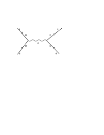
FIG. 16.: Contributions to Im($\Delta M_{12}$) by aspon exchange (Circles mean mixings.)

We obtain

$$Im(M_{12})=\frac{f_{K}^{2}m_{K}}{6}\frac{1}{\kappa^{2}}Im(x_{1}x_{2}^{*})^{2}$$ (153)

where $\kappa^{2}=\kappa_{1}^{2}+\kappa_{2}^{2}$. The color factor has been taken into account in Eq.(153). Im($M_{12}$) receives contributions from the new $2W$-exchange box diagrams shown in Figure 17,

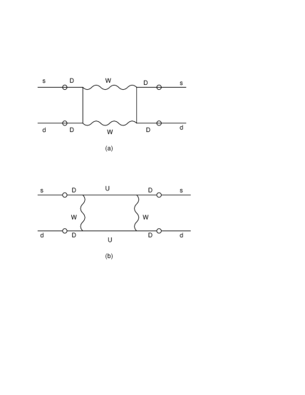
FIG. 17.: Contributions to Im($\Delta M_{12}$) by new quarks and two-W box diagrams. (Circles mean mixings.)

but these contributions are negligible. We will consider the CP-violating parameters, such as $Im(M_{12})/\Delta M_{K}$ in more detail below.

Next we consider the up sector for completeness. We can also choose states such that $M_{up}$ in Eq.(144) is replaced by

$$M_{up}=\left(\begin{array}[]{cccc}m_{u}&0&0&\tilde{F}_{1}\\ 0&m_{c}&0&\tilde{F}_{2}\\ 0&0&m_{t}&\tilde{F}_{3}\\ 0&0&0&M\end{array}\right)$$ (154)

with

$$\tilde{F}_{i}=C_{ij}F_{j}$$ (155)

where C is the real standard $3\times 3$ KM matrix. The transformation matrices ${\bf J}_{L}$ and ${\bf J}_{R}$ that diagonalize $M_{up}$ in Eq.(154) can be related to ${\bf K}_{L}$ and ${\bf K}_{R}$ by changing $x_{i}$ into $\tilde{x}_{i}(=\tilde{F}_{i}/M)$ and $m_{d},m_{s}$ and $m_{b}$ into $m_{u},m_{c}$ and $m_{t}$. The generalized $4\times 4$ KM matrix is given by

$${\bf V}_{KM}^{(4)}={\bf J}_{L}^{\dagger}\left[\begin{array}[]{cc}{\bf C}&0\\ 0&1\end{array}\right]{\bf K}_{L}$$ (156)

Before proceeding, we note that flavor-changing Z-coupling can be induced by the one-loop diagram shown in Figure 18.

FIG. 18.: Flavor-changing Z coupling induced by new quarks at one loop.

By naive dimensional arguments, the effective coupling constant $\beta_{ij}$ is

$$\beta_{ij}=\left(-\frac{1}{2}\right)\frac{g_{2}}{cos\theta_{W}}\frac{h_{i}h_{j}}{16\pi^{2}}\left(\frac{M}{m_{\chi}}\right)^{2}$$ (157)

Using $h_{1,2,3}\simeq 0.01$ and $(M/m_{\chi})^{2}\simeq 0.1$, we conservatively estimate $\beta_{ij}$ to be less than $10^{-7}$. Therefore, we expect these FCNC’s to be smaller than those in the standard model.

Consider now the one-loop corrections to $\bar{\Theta}$. Although the mass matrices in Eq.(144) are complex, their determinants are real. Therefore, $\bar{\Theta}$ defined in Eq.(129) is zero at tree level. $\bar{\Theta}$ will be nonzero when the mass matrices receive radiative corrections. For example, the contributions to $\bar{\theta}$ from the up sector are given by

$$\bar{\Theta}(up) = Arg[det(M_{up}+\delta M_{up})]$$ (158)

$$= ImTrln[M_{up}(1+M_{up}^{-1}\delta M_{up})]$$ (159)

$$\simeq ImTr(M_{up}^{-1}\delta M_{up}),$$ (160)

where we have used the fact that $M_{up}$ is real and that the corresponding radiative corrections $\delta M_{up}$ are small. The last line in Eq.(160) is valid at one-loop order. Defining the one-loop corrections $\delta M_{up}$ by

$$\delta M_{up}=\left(\begin{array}[]{cc}\delta{\bf m}_{u}&\delta{\bf F}\\ \delta{\bf m}_{Uu}&\delta M\end{array}\right)$$ (161)

and combining with Eq.(160), we obtain

$$\bar{\Theta}(up)=ImTr({\bf m}_{u}^{-1}\delta{\bf m}_{u}-{\bf m}_{u}^{-1}{\bf F}M^{-1}\delta{\bf m}_{Uu}+M^{-1}\delta M).$$ (162)

Notice that $\delta F$ will not contribute to $\bar{\Theta}$ at one-loop order because of the structure of $M_{up}$. The expression for $\bar{\Theta}(down)$ is strictly analogous to Eq.(162).

By studying all possible one-loop diagrams[62, 246] we find that the only contribution to $\bar{\Theta}$ comes through $\delta{\bf m}_{u}$ in Eq.(162) and, in particular, from the diagram depicted in Figure 19. The imaginary part gives a contribution

$$\bar{\Theta}(up)=\frac{1}{\sqrt{2}}\frac{1}{(4\pi)^{2}}\sum_{\alpha=1,l=1}^{\alpha=2,l=3}h_{l}^{\alpha}Im[x_{l}^{*}]\lambda_{\alpha}\frac{\kappa}{M}$$ (163)

FIG. 19.: One loop diagram of which the imaginary part contributes to $\overline{\Theta}$.

which gives the estimate (for convenience we shall write x to denote $x=|x_{i}|$, the modulus, and taken to be generation independent since the limits on $x$ are not sensitive to the generation considered)

$$\bar{\Theta}=\frac{\lambda x^{2}}{16\pi^{2}}$$ (164)

Here $\lambda_{\alpha}$ is the coefficient of the quartic interaction between the two types of Higgs $|\phi|^{2}|\chi_{\alpha}|^{2}$, and $\lambda$ with no subscript is an average value. (Actually there are three independent $\lambda$ corresponding to indices 11, 12+21, 22 but our estimates will not distinguish these).

As mentioned earlier, the neutron electric dipole moment $d_{n}$ has been calculated[213, 214] in terms of $\bar{\Theta}$ long ago with the result that

$$d_{n}\simeq 10^{-15}\bar{\Theta}e.cm.$$ (165)

and so we know from $d_{n}\leq 10^{-25}$ e.cm. empirically that $\bar{\Theta}\leq 10^{-10}$, from which it follows by Eq.(164) that $\lambda x^{2}$ is less than $10^{-8}$.

In the kaon system, the CP violation parameter $|\epsilon_{K}|$ is given[62, 245] by

$$|\epsilon_{K}|=\frac{1}{\sqrt{2}\Delta m_{K}}m_{K}\frac{f_{k}^{2}}{3}\frac{2}{\kappa^{2}}x^{4}$$ (166)

Using $(\Delta m_{K}/m_{K})=7.0\times 10^{-15}$, $f_{K}=0.16$GeV gives the relationship between $x^{2}$ and the $U(1)_{new}$ breaking scale

$$\kappa/x^{2}=2.9\times 10^{7}GeV$$ (167)

Thus, if we insist that the $U(1)_{new}$ is broken above the electroweak breaking scale ($\sim 250GeV$) then

$$x^{2}\gtrsim 10^{-5}$$ (168)

From Eq.(164), this means that $\lambda<10^{-3}$.

In [243], it was argued plausibly that $\lambda>10^{-5}$ on the basis of naturalness; this would imply that $\bar{\Theta}>10^{-12}$ and hence $d_{n}>10^{-27}e.cm.$

But we can find a yet more solid and conservative lower bound on $d_{n}$. It follows from the fact that the $|\phi|^{2}|\chi_{\alpha}|^{2}$ interaction receives a one-loop correction from the quark loop box diagram where three sides are the top quark and the fourth is the heavy $U$-quark (see Figure 20).

FIG. 20.: One loop $|\phi|^{2}|\chi|^{2}$ counterterm for the coupling $\lambda$.

The full $\lambda$ is given by

$$\lambda=\lambda_{tree(bare)}+\lambda_{1-loop}(\mbox{including counterterm})+\mbox{higher loops}$$ (169)

and the one-loop finite contribution, for the dominant diagram, Figure (20), neglecting quark masses and taking $h_{3}^{\alpha},g_{t}$ as the respective Yukawa copuplings to $\chi_{\alpha}$ and $\phi$ of the third generation by

$$\lambda_{1-loop}\simeq\int\frac{d^{4}k}{(2\pi)^{4}}|h_{3}^{\alpha}|^{2}|g_{t}|^{2}\frac{1}{k^{4}}+\mbox{counterterm}$$ (170)

which imples that the lowest value for $\lambda$ (without accidental cancellations) is:

$$\lambda\gtrsim\frac{x^{2}}{16\pi^{2}}$$ (171)

Combining Eqs.(164) and (171) then gives the estimate for $\bar{\Theta}$ of

$$\bar{\Theta}\gtrsim\frac{x^{4}}{16\pi^{4}}$$ (172)

which implies that $x^{2}\leq 10^{-3}$ (incidentally in full agreement with [243]) and that $10^{-10}\geq\bar{\Theta}\geq 10^{-14}$.

From Eq.(165), this then gives a lower limit on the neutron electric dipole moment of

$$d_{n}\geq 10^{-29}e.cm.$$ (173)

This is more than two orders of magnitude greater than the prediction of the KM mechanism and thus provides another distinguishing feature of spontaneous CP violation.

Before addressing other consequences of the Aspon Model, let us point out that the production of the predicted heavy quarks and the aspon in a hadron collider is discussed in Ref. [240].

A promising approach to finding new quark flavors is through searching for heavy quark bound states. This fails for the top quark since the single $t$ quark decay to $bW$ is more rapid than the formation time of toponia. However, the $Q$ of the Aspon Model have a very much longer lifetime because of the small mixing with the three light generations. Such production of the exotic quarkonia is dicussed in [32].

The experimental information regarding CP violation still comes primarily from the neutral kaon system and is inadequate to determine whether the KM mechanism is the correct underpinning of CP violation. In dedicated $B$ studies, with more than $10^{8}$ samples of $B^{0}(\bar{B}^{0})$ decay, it will be possible[247, 248, 249, 250, 251] to test this assumption stringently by measuring the angles of the well-known unitarity triangle whose sides correspond to the complex terms of Eq.(127). If CP is spontaneously broken, as in the Aspon Model, the outcome of these measurements will be different from the predictions of the standard model.

The three angles of the unitarity trangle are conventionally defined as $\alpha,\beta$, and $\gamma$ between the first and second, second and third, third and first sides in Eq.(127) respectively. These angles can be separately measured for the standard model by the time-dependent CP asymmetry

$$a_{f}(t)=\frac{\Gamma(B^{0}(t)\rightarrow f)-\Gamma(\bar{B}^{0}\rightarrow f)}{\Gamma(B^{0}(t)\rightarrow f)+\Gamma(\bar{B}^{0}\rightarrow f)}$$ (174)

where the final state $f$ is a CP eigenstate. We define $q,p$ in $B^{0}-\bar{B}^{0}$ mixing by the mass eigenstates $B_{1,2}$:

$$|B_{1,2}>=p|B^{0}>\pm q|\bar{B}^{0}>$$ (175)

and similarly for $K_{1,2}$ in the kaon system. Also, $A,\bar{A}$ are the decay amplitudes

$$A,\bar{A}=<f|H|B^{0},\bar{B}^{0}>$$ (176)

. Let us consider the specific cases of $f=\pi^{+}\pi^{-},\psi K_{S}$ from $B_{d}$ decay and $f=\rho K_{S}$ from $B_{s}$ decay. We define $\lambda(f)$ by

$$\lambda(\pi^{+}\pi^{-})=\left(\frac{q}{p}\right)_{B_{d}}\left(\frac{\bar{A}}{A}\right)_{B_{d}\rightarrow\pi^{+}\pi^{-}},$$ (177)

$$\lambda(\psi K_{S})=\left(\frac{q}{p}\right)_{B_{d}}\left(\frac{\bar{A}}{A}\right)_{B_{d}\rightarrow\psi K}\left(\frac{q}{p}\right)_{K},$$ (178)

and

$$\lambda(\rho K_{S})=\left(\frac{q}{p}\right)_{B_{s}}\left(\frac{\bar{A}}{A}\right)_{B_{s}\rightarrow\rho K}\left(\frac{q}{p}\right)_{K}^{*}.$$ (179)

The complex conjugate appears in Eq.(179) because $B_{s}^{0}\rightarrow\bar{K}^{0}$ while $B_{d}^{0}\rightarrow K^{0}$. If to a sufficiently good approximation $|q/p|=1$ and $|\bar{A}/A|=1$, as we shall show for the Aspon Model below, then $\lambda(f)$ is related to the CP asymmetry through the $B_{1}-B_{2}$ mass difference $\Delta M$ by

$$a_{f}(t)=-\mbox{Im}\lambda(f)\mbox{sin}(\delta Mt).$$ (180)

In the standard model the angles of the unitarity triangle are related to the $\lambda(f)$ by:

$$\mbox{sin}2\alpha=\mbox{Im}\lambda(\pi^{+}\pi^{-});\hskip 14.45377pt\mbox{sin}2\beta=\mbox{Im}\lambda(\psi K_{S});\hskip 14.45377pt\mbox{sin}2\gamma=\mbox{Im}\lambda(\rho K_{S}).$$ (181)

Such relations are no longer valid in the Aspon Model because $Im(q/p)_{B_{d}}$ has a major contribution from aspon exchange and $Im(q/p)_{K}$ is dominated by aspon exchange.

To evaluate the CP asymmetries in B decays for the Aspon Model one needs to evaluate the different factors in the $\lambda(f)$ given in Eqs.(177) - (179) above. More precisely we need, from Eq.(180), the imaginary part of the $\lambda(f)$. The Aspon Model adds new Feynman diagrams involving aspon exchange to those already present in the standard model. Because CP is only spontaneously broken, the W-exchange amplitudes are predominantly real amd have very small phases while the aspon exchange has a much smaller magnitude but an unpredicted arbitrary phase. As a result, the $|\mbox{Im}\lambda(f)|$ appearing in Eq.(180) are of order $0.002$ or less, compared to the standard model expectation that $|\mbox{Im}\lambda(f)|$ be of order of, although less than, unity. Thus CP asymmetries in B decays are predicted to be correspondingly smaller than in the standard model. The technical details can be found in Ref. [242].

It is found, setting $M_{A}=300$ GeV, that

$$|\mbox{Im}\lambda(\pi^{+}\pi^{-})|\leq 1\times 10^{-5},$$ (182)

$$|\mbox{Im}\lambda(\psi K_{S})|\leq 2\times 10^{-3},$$ (183)

$$|\mbox{Im}\lambda(\rho K_{S})|\leq 2\times 10^{-3}.$$ (184)

The resulting asymmetries $a_{f}(t)$ are much smaller than those predicted by the standard model where these imaginary parts are all of order unity.

It is also interesting to observe from Eqs.(177) - (179) that

$$\frac{\lambda(\psi K_{S})\lambda(\rho K_{S})}{\lambda(\pi^{+}\pi^{-})} = \left(\frac{q}{p}\right)_{B_{s}}\left(\frac{\bar{A}}{A}\right)_{B_{d}\rightarrow\psi K}$$ (185)

$$= \left(\frac{q}{p}\right)_{B_{s}}\left(\frac{\bar{A}}{A}\right)_{B_{s}\rightarrow D_{s}^{+}D_{s}^{-}}$$ (186)

$$= \lambda(D_{s}^{+}D_{s}^{-}).$$ (187)

In the Aspon Model, where the $\lambda(f)$ have unit moduli and $|\mbox{Im}\lambda(f)|\ll 1$, this relation implies a linear relation for the imaginary parts:

$$\mbox{Im}\lambda(\psi K_{S})+\mbox{Im}\lambda(\rho K_{S})-\mbox{Im}\lambda(\pi^{+}\pi^{-})-\mbox{Im}\lambda(D_{s}^{+}D_{s}^{-})=0,$$ (188)

which provides an additional test of the Aspon Model.

In conclusion, our result is that, if the Aspon Model is correct, CP asymmetries in B decays would be much smaller than predicted by the standard model and the relation (188) would be satisfied.

One may ask[243] whether the present experimental situation of B decay is compatible with the Aspon Model?

In the model, the quark mixing matrix is a complex unitary $4\times 4$ matrix $C_{\mu\nu}$. Mixings of the conventional six quarks with one another are specified by the $3\times 3$ matrix $C_{ij}$, whose indices run from 1 to 3. $C_{ij}$ is neither real nor unitary because of $\chi$-induced mixings to the undiscovered quark doublet. However, these terms are $\sim x^{2}$. Thus, since $x^{2}\leq 10^{-3}$, $C_{ij}$ is, to a precision of at least $0.1\%$, a real orthogonal matrix. It is a generalized Cabibbo matrix rather than a Kobayashi-Makawa matrix. This is unfortunate for the search for CP violation in the beauty sector, but has other observable consequences.

In the standard model, the Kobayashi-Maskawa matrix $V$ is complex and unitary. The sides of the unitarity trangle are unity and

$$R_{b}=\left|\frac{V_{ud}V_{ub}}{v_{cd}V_{cb}}\right|,\hskip 21.68121ptR_{t}=\left|\frac{V_{td}V_{tb}}{v_{cd}V_{cb}}\right|.$$ (189)

The value of $R_{b}$ has been measured. According to [251], $R_{b}=0.35\pm 0.09$. The value of $R_{t}$ cannot be extracted from experimental data alone. Appeal must be made to a theoretical evaluation of the neutral B-meson mass difference using the standard model. The analysis in [251] yields $R_{t}=0.99\pm 0.22$. These results suggest a rather large value of the CP-violating angle $\beta$, namely, $0.34\leq\beta\leq 0.75$.

In the Aspon Model, the matrix $C_{ij}$ is orthogonal up to terms of order $x^{2}$ arising from mixings with unobserved quarks. Thus, we anticipate no readily observable manifestations of CP violation in the beauty sector. Furthermore, the unitarity triangle must degenerate into a straight line: $|R_{b}\pm R_{t}|=1$. In this case, we cannot appeal to a theoretical calculation of the neutral B-meson mass difference since it depends on unknown parameters. On the other hand, the matrix $C_{ij}$ with neglect of terms $\sim x^{2}$ involves only three parameters. ¿From data at hand, in this context, we obtain $R_{t}=1-\rho$ in the Wolfenstein[252] parametrization, whence $R_{t}=0.637\pm 0.09$. We note that present data yields $R_{b}+R_{t}=0.99\pm 0.13$. This result is compatible with an approximately orthogonal mixing matrix and hence with the Aspon Model.

As a final CP violation parameter in the Aspon Model, we shall discuss the value predicted for Re$\left(\frac{\epsilon^{{}^{\prime}}}{\epsilon}\right)$ - a measure of direct CP violation in K decay. To evaluate Re$\left(\frac{\epsilon^{{}^{\prime}}}{\epsilon}\right)$ requires the study of several Feynman diagrams[253, 254, 255, 256, 257, 258], and their comparison to the standard model. Recall that the most recent evaluations completed at CERN (NA31) [259] and FNAL (E371) [260, 261] give results Re$\left(\frac{\epsilon^{{}^{\prime}}}{\epsilon}\right)=(23\pm 3.6\pm 5.4)\times 10^{-4}$ and Re$\left(\frac{\epsilon^{{}^{\prime}}}{\epsilon}\right)=(7.4\pm 5.2\pm 2.9)\times 10^{-4}$ respectively, where the first error is statistical and the second is systematic. These results are consistent within two standard deviations; the error is expected to be reduced to $1\times 10^{-4}$ in foreseeable future experiments.

A detailed analysis of $\epsilon^{\prime}/\epsilon$ in the Aspon model was carried out by Frampton and Harada[245, 246]. They showed that penguin diagrams involving the additional quarks give the dominant contribution. The outcome of these considerations is that Re$\left(\frac{\epsilon^{{}^{\prime}}}{\epsilon}\right)$ is not larger than $10^{-5}$ in the Aspon Model. While it does not vanish exactly, it does correspond closely to a superweak model prediction[264].

This discussion of the Aspon Model is presented as a motivation for additional quarks beyond the six discovered flavors. Because of the smallness of $x^{2}$ which characterizes the mixing of the additional quarks with the known ones, the new quarks have a long lifetime. This is important in their experimental detection, as discussed the next Section.

VII Experimental Searches.

A Search for long-lived quarks

1 Present Searches

The search for long-lived quarks is an ongoing process at the Fermilab Tevatron. The first search at the Tevatron was made by the D0 collaboration [265] which looked for signals $b^{\prime}\rightarrow b\gamma$, where $b^{\prime}$ is a charge -1/3 quark, setting a limit $m_{b^{\prime}}>M_{Z}+m_{b}$. The second and most recent search was made by the CDF collaboration[266] which looked for a displaced vertex for $Z\rightarrow e^{+}e^{-}$ coming from $b^{\prime}\rightarrow bZ$ resulting in $m_{b^{\prime}}>148$ GeV (for $c\tau=1$ cm.). The latter search will be described below. Eventually, such a search will be carried out at the LHC which has a much greater C.M. energy, with a much larger production cross section. In this section, we will concentrate on the current limits coming out of two operating facilities: LEP2 and Fermilab. In the next section, we will discuss the prospects for future searches, both at the Fermilab Tevatron and at the LHC. We will only briefly discuss prospects for such a search at facilities which are under discussion, such as the NLC, etc. Also in this section, we will focus primarily on hadron colliders such as the Tevatron since these are the machines which can explore the mass range that was discussed earlier.

In the search for a new particle, there are two principal activities to attend to: how to produce the particle and how to detect it. For a particle which is somewhat “exotic”, such as supersymmetric particles, the production process would be highly model-dependent. Fortunately, for a heavy quark, this is rather standard: it proceeds through the $q\bar{q}$ and $gg$ channels. For the range of heavy quark masses considered in this Report, the $q\bar{q}$ process via the electroweak channels $W,\gamma,Z$ is completely negligible compared with the QCD process with gluons. The production cross section, at the Tevatron and at the LHC, for the top quark as a function of its mass has been computed up to the next-to-leading order in QCD [267]-[272]. (The $q\bar{q}$ channel is dominant at the Tevatron while the $gg$ channel is dominant at the LHC.) This can be directly applied to the present search for long-lived quarks whose production mechanism should be similar to that of the top quark. The production cross sections as a function of the heavy quark mass are shown in Figs. 21 and 22 for the Tevatron at $\sqrt{s}=1.8$ TeV and 2 TeV respectively, and in Fig. 23 for the LHC at $\sqrt{s}=10,14$ TeV. Here “$m_{t}$” will stand for a generic heavy quark mass, for both the Tevatron and the LHC.

FIG. 21.: Physical cross section for $p\overline{p}\rightarrow t\overline{t}X$ at $\sqrt{s}=1.8$ TeV as a function of the top mass. This cross section applies to a heavy quark $Q$ as well with $t$ changed to $Q$. The two data points are from CDF and D0 respectively for the top quark.

FIG. 22.: Physical cross section for $p\overline{p}\rightarrow t\overline{t}X$ at $\sqrt{s}=2.0$ TeV as a function of the top mass. This cross section applies to a heavy quark $Q$ as well with $t$ replaced by $Q$.

FIG. 23.: Cross section for $pp\rightarrow t\overline{t}X$ at $\sqrt{s}=10$ and $14$ TeV as a function of the top mass. Notice that $p$ has been mislabeled as $\overline{p}$ in the figure. The same prediction applies to a heavy quark $Q$.

As can be seen above, the predicted cross section at the LHC, for a given heavy quark mass, exceeds that at the Tevatron by more than two orders of magnitude, which will facilitate the search for such an object.

The next task is to define the detection capability of various detectors. Since the latest constraint on long-lived quarks come from CDF [266], we shall use it as a prototype of detectors dedicated to such a purpose. Other detectors such as D0 are very similar in layout. Needless to say, the CDF detector is a complicated, multipurpose one whose specifications can be found in [273]. A generic detector for hadron colliders generally consists of a (silicon) vertex detector immediately surrounding the beam pipe for high precision determination of the location of the tracks. Next comes a central tracking chamber which measures charged tracks and momenta of charged particles. Surrounding these two units are generally hadron calorimeters which measure the energy deposited by hadrons. Next comes the muon chambers which detect the location of the particles which penetrate the calorimeters. As described below, the first two parts (vertex detector and central tracking chamber) were used to search for displaced vertices coming from the decay of a long-lived particle. For stable or very long lived particles, the muon chambers are used in conjunction with the ionization energy loss in the tracking chambers to make such a search.

The current search at CDF can be divided into two categories: the search for those quarks whose decay lengths, $l=\gamma\beta c\tau$ with $\tau$ being the proper decay time, is 1) less than 1 meter, and 2) greater than 1 meter.

Let us first concentrate on the first category ($l<1$ meter) [266]. The parts of the detector which are relevant here consist of two components: a silicon vertex detector immediately surrounding the beam pipe for precision tracking and a central tracking chamber embedded in a 1.4 T solenoid magnetic field which measures the momenta and trajectories of charged particles. In the search for a new particle, a crucial task would be the identification of a characteristic signature which would distinguish it from background. In the present case, that characteristic signature is the decay $Z\rightarrow e^{+}e^{-}$ with the $e^{+}e^{-}$ vertex displaced from the $p\overline{p}$ interaction point. This $Z$ boson could come from the decay of a charge -1/3 quark (denoted by $b^{\prime}$ in Ref.[266] and by $D$ in Ref. [188] in the process $D\rightarrow b+Z$ with a subsequent decay $Z\rightarrow e^{+}e^{-}$. In this case, $D$ would be the long-lived parent of the $Z$ boson. The search at CDF concentrated on events containing an electron-positron pair whose invariant mass is consistent with the $Z$ mass and whose vertex is displaced from the $p\overline{p}$ interaction point. The data used was from the 1993-1995 Tevatron run with an integrated luminosity of $90\,pb^{-1}$ of $p\overline{p}$ collisions at $\sqrt{s}$ = 1.8 TeV.

In the search for a long-lived parent of the $Z$, the CDF collaboration focused on the measurement of $L_{xy}$ which is the distance in the transverse ($r-\phi$) plane between the $p\bar{p}$ interaction point and the $e^{+}e^{-}$ vertex. Notice that $L_{xy}=\gamma\beta_{xy}c\tau$ with $\beta_{xy}$ being the transverse component of the parent particle didived by $c$. As defined by the CDF collaboration, $L_{xy}$ can be either positive or negative. For prompt $Z$’s coming from the SM process $q\overline{q}\rightarrow Z\rightarrow e^{+}e^{-}$, one would expect $L_{xy}\approx 0$ because of the short lifetime of the $Z$. The $L_{xy}$ distribution with appropriate cuts taken into account is shown in Fig. 24 below

FIG. 24.: The $L_{xy}$ distribution of the Z’s after applying all cuts. The data are represented by the circles. The histogram is the expected $L_{xy}$ distribution for prompt Z’s based on the measured $L_{xy}$ uncertainty in the event sample. The inset shows the distribution after the 2 jet requirement is applied. The vertical dashed lines separate the prompt and non-prompt regions.

As emphasized by [266], this distribution is consistent with that for prompt $Z$’s where one would expect less than one event for $|L_{xy}|<0.1$ cm. [266] also pointed out that the number of events with $L_{xy}$ significantly less than zero is an effective measure of the background. The CDF collaboration observed one event for $L_{xy}>0.1$ cm and 3 events for $L_{xy}<-0.1$ cm. As stated, there is no evidence for a long-lived parent of the Z. This is shown in Fig. 25 where the constraint is expressed in terms of the 95 level upper limit on the product of the production cross section for the long-lived parent, $\sigma_{X}$, its branching ratio, Br($X\rightarrow Z$), the branching ratio, Br($Z\rightarrow e^{+}e^{-}$), and the $e^{+}e^{-}$ acceptance for pseudorapidity $|\eta|<1$.

FIG. 25.: The 95% confidence level upper cross section limit for $\sigma.Br$ times the acceptance for an electron-positron pair to be within the detector as a function of fixed $\lambda_{xy}\equiv\gamma\beta_{xy}c\tau$. Cross sections above the curve have been excluded at the 95% confidence level. The inset shows the exclusion curve and the theoretical prediction for a $b^{\prime}$ quark of mass 110 GeV as a function of its lifetime, assuming 100% decay into $bZ$.

The above discussions and figures deal with limits on the production of a single parent with its subsequent decay into a $Z$. We are, however, most interested in the detection of a long-lived quark. As we have mentioned earlier, this long-lived quark would be produced in pair. The CDF search for a long-lived $D$ (or $b^{\prime}$) which is pair-produced can be summarized as follows. The kind of events that are searched for would include, besides the $e^{+}e^{-}$ pair coming from the $Z$, two or more jets. For instance, this could come from the reaction: $q\overline{q}\rightarrow D\overline{D}\rightarrow bZ\overline{b}Z\rightarrow be^{+}e^{-}\overline{b}q\overline{q}$. The $L_{xy}$ distribution is shown in the inset of Fig. 25. There one would expect less than one event for $L_{xy}\leq 0.01$ cm. The CDF collaboration found one event. This was then translated into a cross section limit as a function of $c\tau$, where $\tau$ is the lifetime of $D$. Assuming that Br($D\rightarrow bZ$) = $100\%$, the exclusion curve for the $D\bar{D}$ production cross section as a function of $c\tau$ is shown as an inset of Fig. 25 for a $D$ quark of mass 110 GeV. The theoretical prediction for the cross section for such a mass is shown as a horizontal line. Clearly, this is ruled out for a wide range of lifetimes. For other masses, the exclusion curves for the cross section are not shown but are instead translated into exclusion regions in the mass-lifetime plane. (This is because the production cross section can be calculated in QCD as a function of the $D$ mass as mentioned above.) The plot shown in Fig. 26 assumes the above branching ratio.

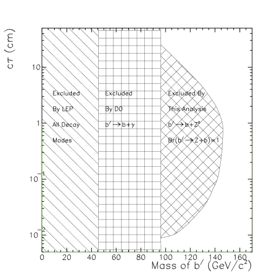
FIG. 26.: The hatched areas in this plot represent the 95% confidence-level regions of $b^{\prime}$ mass and lifetime that have been excluded. For $c\tau=1$ cm, CDF excluded up to a mass of $148$ GeV.

In Fig. 26, three forbidden regions are presented: the LEP, the $D0$, and the CDF constraints. The most stringent constraint comes, of course, from the CDF results. As can be seen from Fig. 26, for every $c\tau$, there is a range of forbidden masses represented by the shaded region. The largest forbidden range is for $c\tau$ = 1 cm corresponding to a lifetime $\tau\approx 3.3\times 10^{-11}$ sec . This rules out the mass of the $D$ quark up to 148 GeV. For smaller or larger $c\tau$, we can see that the lower bounds on the $D$ mass become somewhat smaller than 148 GeV . If the $D$ quark, happens to have a mass larger that 148 GeV, it could escape detection for a large range of lifetimes as can be seen in Fig. 26. The mere fact that there exists unexplored regions of the detector, as shown in the unshaded areas of Fig. 26, is reason to believe that there are plenty of opportunities for future searches.

What does this result tell us about the long-lived quarks with the mass range that we have discussed in Section IV? First, as we have mentioned earlier, we are especially concerned with the mass of the heavy quarks larger than 150 GeV. From Fig. 26, one can see that the CDF search based on the decay mode $D\rightarrow bZ$ does not set any constraint on long-lived quarks with a mass greater than 150 GeV. In other words, if this long-lived quark exists and if it decays at a distance $L_{xy}>$ 0.01 cm, it has yet to be discovered. This statement is, of course, based on the assumption that the branching ratio for $D\rightarrow bZ$ is $100\%$. As discussed in Section IV and in Ref. [188], for $m_{D}\leq m_{t}$, there is another possible decay mode for $D$, namely $D\rightarrow(c,u)W$ (the $c$ quark channel in any reasonable scenario dominates over the $u$ quark channel). Whether or not $D\rightarrow bZ$ dominates over $D\rightarrow cW$ will depend on a particular model for the mixing element $|V_{Dc}|$. As discussed in Ref. [188], even with a very naive assumption $|V_{Dc}|\sim x^{3/2}$, with $x$ being the mixing parameter between the third generation and the heavy quark, $D\rightarrow bZ$ can dominate over $D\rightarrow cW$ for a certain range of mass and mixing $x$. For $|V_{Dc}|\sim x^{2}$ (or less), the $bZ$ mode will almost always be the dominant one. Since this is a rather model-dependent statement, one should, in principle, look for both modes when $m_{D}\leq m_{t}$. Unfortunately, the mode $D\rightarrow cW$ would be rather difficult to detect. We shall come back to this issue and others in the discussion of future searches.

The next question concerns the limits on a charged “stable” or very long-lived massive particle. Such a search is being carried out a CDF. Basically, this search focuses on decay lengths larger than 1 m, i.e. larger than the radius of the Central Tracking Chamber. As of this writing, preliminary results have only appeared in conference talks, [113, 114]. Therefore, what is described below will be considered preliminary. A stable massive quark moving at a low velocity will leave an ionization track in the tracking chamber because the energy loss $dE/dx\propto 1/\beta^{2}$ (the Bethe-Bloch equation) and a low $\beta$ would imply a large energy loss. Furthermore, for such a stable massive quark to be detected, one would look for signals in the muon detector after mesons formed from this particular quark have traversed the calorimeters and reached the muon detector. To distinguish it from a muon, one would have to correlate this signal with the large energy deposited in the tracking chamber. The measurement of $dE/dx$ as a function of $\beta\gamma=p/M$, combined with the momentum measurement would allow for a determination of the mass of the particle. The mass limits from CDF for such a very long-lived quark are approximately 200 GeV.

In summary, the most stringent limits, so far. on long-lived quarks come from the CDF collaboration [266]. It excludes a long-lived, charge -1/3 quark of mass up to 148 GeV for a lifetime $\tau\approx 3.3\times 10^{-11}$ sec ($c\tau$ = 1 cm). For other values of lifetimes, the excluded mass ranges are weaker as can be seen in Fig. 26. This constraint was based on the search for a displaced vertex for the decay $Z\rightarrow e^{+}e^{-}$ which could come from the decay $D\rightarrow bZ$. Furthermore, all of these constraints come from the search for the decay of the $D$ quark inside the Central Tracking Chamber. If the $D$ quark lives long enough to enter the calorimeters and subsequently trigger a signal in the muon chamber, the constraint (which is preliminary) is much stronger: a $D$ quark mass below approximately 200 GeV is excluded. In short, under what circumstances will a $D$ quark escape detection so far? First, if its mass is above 148 GeV (as referred to in Section IV) and if it decays inside the Central Tracking Chamber. If the mass is above $\sim$ 200 GeV, $D$ is no longer required to decay in the tracking chamber: it simply escapes detection regardless of where it decays. Most of the discussion in Section IV concerned these possibilities.

What kind of improvements should be made in order to be able to search for these quarks heavier than 148 GeV which could either decay inside the Central Tracking Chamber or, if heavier than 200 GeV, could also travel through the calorimeters? What about the $U$ quark? How could one detect it? What if the dominant decay mode of the $D$ is $D\rightarrow cW$? These are the kinds of questions that one would like to address, at least qualitatively, in the next section.

2 Future Searches

The first kind of future searches would be based on present facilities such as the Tevatron. In particular, one might ask what kind of improvement one can make by exploiting the present CDF RunI data with up to 120 $pb^{-1}$. One can then ask what light RunII with a large improvement in luminosity and detector might shed on the search for long-lived quarks.

The above search has focused on the discovery of displaced vertices for decay lengths greater than 100 $\mu m$, with the resulting constraints as described above. What if the decay length is less than 100 $\mu m$? The appropriate kind of experiment would be a counting experiment which is not based on the search for displaced vertices [274]. How feasible this kind of experiment might be will probably depend on the improvements planned for RunII.

These improvements include: a) a detector upgrade with, among several things, added layers of silicon; b) an increase by a factor of 20 in the luminosity. The radius of the silicon vertex detector is roughly of the order of 22.3 cm. Added silicon layers would increase that radius to about 28 cm [274] and consequently the tracking ability of the detector.

For decay lengths between 100 $\mu m$ and 1 m, one of the most important tasks would be to improve the tracking efficiency of the Central Tracking Chamber by adding,for instance, more silicon layers to the vertex detector. Decay lengths of a few tens of cm might be hard, although possible, to detect because of poor tracking efficiency in such a region. This would require new reconstruction algorithm.

The search for very long-lived or “stable” quarks will also be improved by the detector upgrade and the increase in luminosity.

One might ask what else could be done at CDF and D0 in the next run beside those issues discussed above. In particular, one would like to know how feasible might the detection of a signal such as $D\rightarrow cW$ be if it happens to be the dominant decay mode of the $D$. Needless to say, such a task would be much more daunting than the detection of $D\rightarrow bZ$. Nevertheless, a feasibility study would probably be extremely useful. As we have discussed at length in Section IV and in Ref. [188], there is also the partner of the $D$, namely the charge 2/3 quark denoted by $U$, which should not be forgotten. If $U$ is heavier than $D$- but not by much because of the $\rho$-parameter constraint- it will decay into $D$ via $U\rightarrow D+(l^{+}\nu,q_{2/3}\bar{q}{-1/3})$, where particles inside the brackets denote light quarks or leptons or it can decay via $U\rightarrow bW$, depending on how degenerate $U$ and $D$ are and how large $|V_{Ub}|$ is. For the first mode, it was shown in Ref. [188] that $U$ practically decays near the interaction point, with a decay length typically of the order of $10^{-5}\mu m$. The $D$ will subsequently decay between $100\mu m$ and 1 $m$. It will be a challenge to be able to identify such a signal. For the second mode $U\rightarrow bW$, one has to be able to distinguish it from a signal coming from top decay. It would be extremely hard, if not impossible, to be able to resolve the decay vertex to distinguish $U$ from $t$. However, by comparing the predicted number of $t$’s with the observed ones, one might rule out the mode $U\rightarrow bW$ with a $U$ mass close to the top mass.

Turning our attention to the upcoming experiments at the LHC, we would like to briefly describe the two main detectors which will be crucial to the search for long-lived quarks (if such a search would be carried out). They are the Compact Muon Solenoid (CMS) and a Toroidal LHC Apparatus (ATLAS) detectors [275]. The layout for both detectors is generically very similar to CDF and D0.

In the search for long-lived quarks, the components which are crucial would be the central tracking system of CMS and the inner detector of ATLAS. The central tracking system of CMS consists of silicon pixels, silicon and gas microstrip detectors with high resolutions. (The resolution of the silicon pixels is about 11-17 $\mu m$ while the outermost part of the detector, namely the gas microstrip detector, has a resolution of approximately 2$mm$!) The silicon pixels and silicon microstrips cover a radial region up to about 40 $cm$, a marked improvement over the CDF vertex detector. The microstrip gas chamber covers a radial region to approximately 1.18 $m$ which is roughly similar to that covered by the Central Tracking Chamber of CDF.

The inner detector of ATLAS consists of a Semi-Conductor Tracker (SCT): pixel detectors, silicon microstrips and GaAs detector, and Microstrip Gas Counters (MSGC). The pixel detectors have a spatial resolution of about 14 $\mu m$ while the MSGC have a resolution of about 1.8 $mm$, very comparable to CMS. The SCT part covers a radial region of up to 60 $cm$ while the MSGC covers a radial region of up to 1.15 $m$. Again one sees a marked improvement over CDF in the region of interest.

In addition, as can be seen from Fig. 23, the production cross section for a given mass is now increased by at least two orders of magnitude at the LHC because the center of mass energy is now 14 TeV. Such an increase in the cross section combined with the increase in the radial distance covered by silicon detectors would, in principle, help in the search for long-lived quarks. One might wonder if a similar analysis as the one preformed by CDF could be carried over to the LHC experiments. Considering the fact that, with a much higher energy and consequently larger cross section, the number of events and background will be significantly higher as well. This would probably require a different search algorithm.

Finally, concerning proposed but not yet approved colliders such as the Next Linear Collider (NLC) with $\sqrt{s}=500$ GeV, the long-lived quarks with the mass range discussed in Section IV, would be produced copiously and with little background. What kind of signal would one search for will depend on the kind of detectors involved. Whether or not the existence (or nonexistence thereof) of these long lived quarks will be established by CDF, ATLAS, or CMS by the time the NLC operates (if approved) remains an open question.

B Lepton Searches

Earlier in this Report, indirect bounds on the masses of heavy leptons arising from violations of $e-\mu-\tau$ universality were discussed. The bounds were very sensitive to the mixing angle between the third and fourth generations. In this section, we discuss direct detection of heavy leptons.

All current experimental bounds on heavy leptons come from experiments at electron-positron colliders. This is not surprising; the cross section for heavy lepton production at hadron colliders is small and backgrounds are large. Of course, once LEP200 shuts down in a couple of years, the only available colliders for searching for heavy leptons will be the Tevatron and the LHC. We will first examine the current bounds on heavy lepton masses, and then turn towards the future.

It is generally believed that charged heavy leptons can be excluded up to the approximate kinematic limit of LEP. This is not necessarily the case however; the charged heavy leptons of many of the most interesting models have not been excluded for masses above approximately 45 GeV. Below 45 GeV, heavy leptons (charged or neutral) would contribute to the decay width of the $Z$, and such leptons can be excluded.

The strongest bounds on heavy lepton masses reported by LEP have been reported by OPAL[276] and by L3[277]. Both experiments assume that the heavy leptons decay via the charged current decay—the decay $E\rightarrow\tau Z$, which can be large in vectorlike models, is not considered (since it seldom dominates the charged current decay, their bounds are not affected). In the OPAL analysis, they exclude charged leptons which decay via $E\rightarrow\nu_{l}W$ with masses below 80.2 GeV, and those which decay via $E\rightarrow NW$ with masses below 81.5 GeV. Unfortunately, this latter decay assumes that the mass difference between the $E$ and the $N$ is greater than 8.4 GeV. As we have seen in earlier sections, vectorlike models have mass splittings on the order of a few hundred MeV, and even in chiral models, the splitting could also be small. Note, however, that if the mixing angle between the third and fourth generation is bigger than $10^{-6}$, then the $E\rightarrow\nu_{l}W$ would occur near the vertex, and the OPAL bound would apply. The bound was obtained for LEP at $\sqrt{s}=170-172$ GeV, and can be improved somewhat for the later runs.

In the L3 analysis, the mass splitting was assumed to be larger than in the OPAL case, greater than 10 GeV, and similar bounds were obtained. The L3 analysis also looked for long-lived charged leptons, which would exist if the mixing angles with lighter generations were small (typically less than $10^{-7}$) and the charged lepton is lighter than its neutral partner. Of course, such leptons must eventually decay, for cosmological reasons, but we discussed a variety of such scenarios earlier in this Report. L3 excludes such leptons up to a mass of $84.2$ GeV.

Both experiments also looked for heavy neutrinos, which decay at the vertex (mixing angle greater than $10^{-6}$ or so) into a charged lepton and a $W$. For both experiments, the bounds for Dirac (Majorana) neutrinos are approximately $78$ $(66)$ GeV for decays into electrons or muons and $70$ $(58)$ for decays into taus.

So, summarizing the current situation, the bounds on the charged heavy lepton are approximately at the kinematic limit of the collider if and only if this lepton is either stable (i.e. with a lifetime greater than tens of nanoseconds), has a large ($8$ GeV or greater) splitting with its neutrino partner, or has a relatively large mixing angle ($10^{-6}$ or greater) with lighter generations. Note that one of the most interesting models is the $E_{6}$ motivated model with a vectorlike doublet with very small mixing, and this lepton satisfies none of the above conditions. The mass bound for such a lepton is still only given by $Z$ decays. (A search for a nearly degenerate lepton doublet was reported[278] many years ago by the Mark II detector, but only applied for leptons lighter than $10$ GeV.)

Could more analysis at LEP find such a charged heavy lepton? In vectorlike models, the principal decay of the $E$ is into the $N$ plus a very soft pion. It appears to be impossible to pick this pion out of the background from soft tracks from beam-beam interactions. Recently, Thomas and Wells[181] proposed a new signature—triggering on an associated hard radiated photon. This is similar to proposals for counting neutrino species through $e^{+}e^{-}\rightarrow\nu\overline{\nu}\gamma$. At LEP, one would look for $e^{+}e^{-}\rightarrow L^{+}L^{-}\gamma$. There are backgrounds from the above neutrino process, but they can be reduced by looking for a displaced vertex (the decay length is of the oorder of centimeters) and for the soft pions. Thomas and Wells plot the cross section as a function of the $L$ mass and the minimum photon energy. With an integrated luminosity of $240$ pb^-1 at $\sqrt{s}=183$ GeV, and a minimum photon energy of $8$ GeV, they estimate that a doublet mass of up to $70$ GeV could be detected. Presumably, this reach will be considerably higher for the more recent higher energy runs. They note that this signature is unusual for $e^{+}e^{-}$ machines since it is not only limited by the machine energy, but also by the luminosity, and that higher luminosity can significantly extend the reach.

In the chiral case, there remains a “hole” to be filled. If the $E$ is either very close in mass to or lighter than the $N$, it will primarily decay via mixing. If the mixing angle is greater than about $10^{-6}$, then it decays near the vertex and can be detected at LEP up to the kinematic limit. If the mixing angle is smaller than about $10^{-7}$, it is effectively stable and can be detected at LEP up to the kinematic limit. For intermediate angles, the decay length is of the order of tens of centimeters to a meter. Of course, some will still decay near the vertex, and some will decay well within or outside the detector, and so it is possible that a complete analysis could close this hole. Doing so would be useful, since one of the plausible values for the mixing angle discussed in Section III is given by $\sqrt{m_{\nu_{\tau}}/M_{N}}$, which, using $0.01$ eV for the $\nu_{\tau}$ mass, gives $3\times 10^{-7}$ for the mixing angle.

In the future, similar analyses to the above will give similar bounds at lepton colliders near the kinematic limit of the colliders. We have noted, however, that the detection of the vectorlike doublet leptons remains problematic and can best be attacked looking for an associated hard photon. There also seems to be a window for decay lengths of the order of tens of centimeters which has yet to be closed.

The decay mode $E\rightarrow\tau Z$ is generally smaller than the charged current decay–although it is a much cleaner mode, backgrounds are not the problem for $E\rightarrow\nu W$, thus the latter would be detected first. This neutral current decay mode, however, provides a much cleaner signature for hadron colliders, which we now discuss.

A study of searches for heavy charged leptons at hadron colliders was performed by Frampton et al.[182] They considered charged lepton production at the SSC and at the LHC (at 17 TeV). There are two main productin mechanisms for heavy leptons at hadron colliders. The first is gluon fusion, through a triangle graph, into a Higgs boson or a Z-boson. The second is quark fusion directly into a Z-boson (the effects of photon exchange are much smaller than those of the Z). The cross section for lepton production through quark fusion falls off very rapidly as the lepton mass increases, but the cross section through gluon fusion does not fall off as rapidly, since the matrix elements increases as the square of the lepton mass.

First consider the chiral case. Here, gluon fusion dominates for lepton masses above about 150 GeV, and the total cross section for masses between 100 and 800 GeV drops from 0.5 pb to 0.05 pb. This will lead to many thousands of events per year at the LHC. The signature would be a conventional heavy lepton signature. For those masses, and for chiral leptons, one can expect a reasonably large splitting between the $N$ and the $E$, leading to standard single lepton and missing momenta signatures; even if there was an unexpected degeneracy (or if the $N$ were heavier) mixing would lead to clear signatures (note, as discussed above, the importance of closing the window for mixing angles near $10^{-6}$).

What about the vectorlike case? Here, gluon fusion doesn’t contribute, since the leptons don’t couple to the Higgs and the vectorlike coupling to the Z gives no contribution due to Furry’s theorem. Thus, the contributions are only through quark fusion, which fall off much faster. As the lepton mass increases from 100 GeV to 800 GeV, the cross section falls from 1 pb to 0.001 pb. For a 400 GeV heavy lepton, this will give only 1000 events annually at the LHC. This makes detection more difficult, however one should recall that these leptons can decay via the neutral current: $E\rightarrow\tau Z$ which has a branching fraction of at least a few percent (and in some models much larger). This would give a very clear signature with very low background. Even if the decay is suppressed by very small mixing angles, and thus the $E$ passes through the detector, stable lepton searches should see it (it can be readily distinguished from a muon by time-of-flight using the velocity distributions as given in Ref. [182].).

VIII Conclusions.

There are still several reasons to believe that further quarks and leptons remain to be discovered. Although the fourth or further quark-lepton generations cannot be exactly similar and sequential to the first three generations, there are plenty of alternative possibilities which avoid the experimental embarassment to the invisible Z partial width of a fourth light neutrino. The additional quarks and leptons may be chiral as in the first three generastions or non-chiral and vector-like.

The allowed masses are constrained by the precise electroweak data particularly at the Z pole where the data now agree with the minimal standard model at an astonishing 0.1% level. The S, T, U parameters then restrict what states may be added as discussed above in Section (III). Also the stability of the observed vacuum places constraints on additional fermions as does the (optional) requirement of grand unification of the three gauge couplings. Mixing angles for the new quarks and leptons are relatively unconstrained, except by unitarity, without new experimental data.

The lifetime and decay modes (see Section (IV)) of a heavy lepton depend critically on whether the N or E state is the more massive. A similar dependence occurs for heavy quarks which may have such small mixing with the known quarks that at least one new quark may have an exceptionally long lifetime.

In Section (V) we have considered the fascinating possibility that the Higgs boson is not elementary but rather some bound state of additional fermions which transform under the standard gauge group. The heaviness of the top quark has suggested to some that it plays a special role in electroweak symmetry breaking, but even heavier fermions are more attractive candidates to participate in dynamical symmetry breaking.

CP symmetry violation has two disparate but likely related aspects in the Standard Model: the strong CP problem and the weak CP violation in kaon decay. Strong CP can be addressed by addition of extra quarks as explained in our Section (VI). Weak CP violation by the KM mechanism requires at least three generations, and acquires even more CP violating phases in the presence of additional quarks. We have illustrated this with the Aspon model which invokes spontaneous CP violation to relate solution of the strong CP problem by extra vector-like quarks to the violation of CP symmetry in kaon decay. The new vector-like quarks may have long lifetime as mentioned in Section (IV).

Experiment is the final arbitor of everything we have reviewed. Long-lived quarks are being sought at collider facilities. To some extent, detectors have not been designed for such a possibility and this review may encourage further thought in detector design. Similarly heavy leptons are being, and will be, investigated at existing and future colliders.

Discovery of a further quark or lepton would be revolutionary and propel high-energy physics in a new and exciting direction.

This work was supported in part by the US Department of Energy under Grants No. DE-FG02-97ER41036 and DE-A505-89ER40518, and by NSF Grant No. PHY-9600415. We would like to thank David Stuart for many useful discussions about the CDF Collaboration.

REFERENCES

- [1] W. Pauli, personal memorandum (1931).
- [2] F. Reines and C.L. Cowan, Phys. Rev. 113, 273 (1959), and references therein.
- [3] S.H. Neddermeyer and C.D. Anderson, Phys. Rev. 51, 884 (1937)
- [4] J.C. Street and E,C, Stevenson, Phys. Rev. 52, 1002 (1937).
- [5] I.I. Rabi, 1937. Cited in e.g. R.N. Cahn and G. Goldhaber, The Experimental Foundations of Particle Physics. Cambridge University Press (1989) p.52.
- [6] G. Danby, J.-M. Gaillard, K. Goulianos, L.M. Lederman, N. Mistry, M. Schwarz and J. Steinberger, Phys. Rev. Lett. 9, 36 (1962).
- [7] L. Leprince-Ringuet and M. L’héritier, Comptes Rendus Acad. Sciences de Paris, séance du 13 Dec. 1944, p. 618.
- [8] G.D. Rochester and C.C. Butler, Nature 163, 82 (1949).
- [9] R. Brown, U. Camieri, P.H. Fowler, A. Muirhead, C.F. Powell and D.M. Ritson, Nature 163, 82 (1949).
- [10] S.L. Glashow, J. Iliopoulos and L. Maiani, Phys. Rev. D2, 1285 (1970).
- [11] J.J. Aubert et al., Phys. Rev. Lett. 33, 1404 (1974).
- [12] J.E. Augustin et al., Phys. Rev. Lett. 33, 1406 (1974).
- [13] S.C.C. Ting, Rev. Mod. Phys. 44(2), 235 (1977).
- [14] B. Richter, Rev. Mod. Phys. 44(2), 251 (1977).
- [15] G. Goldhaber et al., Phys. Rev. Lett. 37, 255 (1976).
- [16] S.L. Glashow, Nucl Phys. 22, 579 (1961).
- [17] S. Weinberg, Phys. Rev. Lett. 19, 1264 (1967).
- [18] A. Salam, in Elementary Particle Theory, Nobel Symposium, edited by N. Svartholm, Almqvist and Witsell, Stockholm. (1968) p. 367.
- [19] G. ’t Hooft, Nucl. Phys. B33, 173 (1971).
- [20] G. ’t Hooft, Nucl. Phys. B35, 167 (1971).
- [21] N. Cabibbo, Phys. Rev. Lett. 10, 531 (1963).
- [22] M.L. Perl et al, Phys. Rev. Lett. 35, 1489 (1975).
- [23] S.W. Herb et al., Phys. Rev. Lett. 39, 252 (1977).
- [24] Ch. Berger et al. (PLUTO Collaboration) Phys. Lett 76B, 243 (1978).
- [25] F. Abe et al. (CDF Collaboration) Phys. Rev. Lett. 74, 2626 (1995).
- [26] S. Abachi et al. (DO Collaboration) Phys. Rev. Lett. 74, 2632 (1995).
- [27] M. Kobayashi and T. Maskawa, Prog. Theor. Phys. 49, 652 (1973).
- [28] J. Peebles, Ap.J. 146, 542 (1966).
- [29] R.V. Wagoner, W.A. Fowler and F. Hoyle, Ap. J. 148, 3 (1967).
- [30] J. Yang, D.N. Schramm, G. Steigman and R.T. Rood, Ap. J. 227, 697 (1979).
- [31] G. Steigman, K.A. Olive and D.N. Schramm, Phys. Rev. Lett. 43, 239 (1979).
- [32] J. Yang, M.S. Turner, G. Steigman, D.N. Schramm and K.A. Olive, Ap. J. 281, 493 (1984).
- [33] D.N. Schramm and M.S. Turner, Rev. Mod. Phys. 70, 303 (1998).
- [34] G.S. Abramset al. (Mark II Collaboration at SLC) Phys. Rev. Lett. 63, 724 (1989).
- [35] G.S. Abramset al. (Mark II Collaboration at SLC) Phys. Rev. Lett. 63, 2173 (1989).
- [36] B. Adeva et al. (L3 Collaboration at LEP) Phys. Lett. B231, 509 (1989)
- [37] D. Decamp et al. (ALEPH Collaboration at LEP) Phys. Lett. B231, 519 (1989)
- [38] M.Z. Akrawy et al. (OPAL Collaboration at LEP) Phys. Lett. B231, 530 (1989)
- [39] P. Aarinio et al. (DELPHI Collaboration at LEP) Phys. Lett. B231, 539 (1989)
- [40] Particle Data Group, Phys. Rev. D54 (Part 1), 1 (1996), p. 19.
- [41] S.F. King, Phys. Lett. B281, 295 (1992).
- [42] S.F. King, Phys. Rev. D46, R4804 (1992).
- [43] Y. Nambu, in New Theories in Physics, Proceedings of the XI International Symposium on Elementary Particle Physics, Kasimierz, Poland 1988. Editors: Z. Ajduk, S. Pokorski and A. Trautman. World Scientific (1989).
- [44] V.A. Miransky, M. Tanabashi and K.Yamawaki, Mod. Phys. Lett. A4, 1043 (1989)
- [45] V.A. Miransky, M. Tanabashi and K.Yamawaki, Phys. Lett. B221, 177 (1989)
- [46] W.A. Bardeen, C.T. Hill and M. Lindner, Phys. Rev. D41, 1647 (1990).
- [47] K.R. Dienes, E. Dudas and T. Gherghetta, Phys. Lett. B436, 55 (1998) ; Nucl. Phys. B537, 47 (1999) .
- [48] C.D. Carone, hep-ph/9902407
- [49] P.H. Frampton and S.L. Glashow, Phys. Lett. B190, 157 (1987).
- [50] P.H. Frampton and S.L. Glashow, Phys. Rev. Lett. 58, 2168 (1987).
- [51] J.C. Pati and A.Salam, Phys. Rev. D10, 275 (1974).
- [52] R.N. Mohapatra and J.C. Pati, Phys. Rev. D11, 566 (1975).
- [53] G. Senjanovic and R.N. Mohapatra, Phys. Rev. D12, 1502 (1975).
- [54] P.M. Fishbane, S. Meshkov, R.E. Norton and P. Ramond, Phys. Rev. D31, 1119 (1985).
- [55] P.M. Fishbane, K. Gaemers, S. Meshkov and R.E. Norton, Phys. Rev. D32, 1186 (1985).
- [56] P.M. Fishbane, R.E. Norton and M.J. Rivard, Phys. Rev. D33, 2632 (1986).
- [57] R. Foot, H. Lew, R.R. Volkas and G.C. Joshi, Phys. Rev. D39, 3411 (1989) .
- [58] J. Choi and R.R. Volkas, Phys. Rev. D45, 4261 (1992) .
- [59] P. Candelas, G.T. Horowitz, A. Strominger and E. Witten, Nucl. Phys. B258, 46 (1985)
- [60] P.H. Frampton and B.H. Lee, Phys. Rev. Lett. 64, 619 (1990).
- [61] P.H. Frampton and T.W. Kephart, Phys. Rev. Lett. 66, 1666 (1991).
- [62] P.H. Frampton and D. Ng, Phys. Rev. D43, 3034 (1991).
- [63] P.H. Frampton, Phys. Rev. Lett. 69, 2889 (1992).
- [64] F. Pisano and V. Pleitez, Phys. Rev. D46, 410 (1992).
- [65] P. Q. Hung, Phys. Rev. Lett. 80, 3000 (1998).
- [66] M. Veltman, Act. Phys. Pol. B8, 475 (1977).
- [67] M. Veltman, Nucl. Phys. B123, 89 (1977) .
- [68] M. E. Peskin and T. Takeuchi, Phys. Rev. D46, 381 (1992) .
- [69] M. E. Peskin and T. Takeuchi, Phys. Rev. Lett. 65, 964 (1990) .
- [70] G. Altarelli and R. Barbieri, Phys. Lett. B349, 145 (1995) .
- [71] K. Hagiwara, D. Haidt and S. Matsumoto, Eur. Phys. J. C2, 95 (1998).
- [72] J. Erler and P. Langacker, Eur. Phys. J. C3, 90 (1998).
- [73] E. Gates and J. Terning, Phys. Rev. Lett. 67, 1840 (1991) .
- [74] J. Lavoura and L. F. Li, Phys. Rev. D48, 234 (1993) .
- [75] M. Sher, Phys. Reports 179, 273 (1989).
- [76] S. Coleman and E. Weinberg, Phys. Rev. D7, 1888 (1974) .
- [77] M. Bando, T. Kugo, N. Maekawa and H. Nakano, Phys. Lett. B301, 83 (1993) ; Prog. Theor. Phys. 90, 405 (1993).
- [78] C. Ford, D.R.T. Jones, P.W. Stephenson and M.B. Einhorn,Nucl. Phys. B395, 17 (1993) .
- [79] B. Kastening,Phys. Lett. B283, 287 (1992) .
- [80] J.A. Casas, J.R. Espinosa, M. Quiros and A. Riotto, Nucl. Phys. B436, 3 (1995) ; (E)Nucl. Phys. B439, 466 (1995) .
- [81] J.S. Kang, Phys. Rev. D10, 3455 (1974) .
- [82] W. Loinaz and R. Willey, Phys. Rev. D56, 7416 (1997) .
- [83] A. Duncan, W. Loinaz and R. Willey, Phys. Rev. D56, 3874 (1997) .
- [84] D. Boyanovsky, W. Loinaz and R. Willey, Phys. Rev. D57, 100 (1998) .
- [85] I.V. Krive and A.D. Linde, Nucl. Phys. B117, 265 (1976) .
- [86] N.V. Krasnikov, Yad. Fiz 28, 549 (1978).
- [87] P.Q. Hung, Phys. Rev. Lett. 42, 873 (1979) .
- [88] H.D. Politzer and S. Wolfram, Phys. Lett. B82, 242 (1979) ; Phys. Lett. B83, 421 (1979) (E).
- [89] A.A. Anselm, JETP Lett 29, 590 (1989).
- [90] N. Cabibbo, L. Maiani, G. Parisi and R. Petronzio, Nucl. Phys. B158, 295 (1979) .
- [91] R.A. Flores and M. Sher, Phys. Rev. D27, 1679 (1983) .
- [92] M.J. Duncan, R. Philippe and M. Sher, Phys. Lett. B153, 165 (1985) .
- [93] M. Lindner, M. Sher and H.W. Zaglauer,Phys. Lett. B228, 139 (1989) .
- [94] M. Sher,Phys. Lett. B317, 159 (1993) ; Phys. Lett. B331, 448 (1994) . Nucl. Phys. B395, 17 (1993) .
- [95] J.A. Casas, J.R. Espinosa and M. Quiros, Phys. Lett. B342, 171 (1995) ; Phys. Lett. B382, 374 (1996) .
- [96] J.R. Espinosa and M. Quiros, Phys. Lett. B353, 257 (1995) .
- [97] M. Quiros, Perspectives in Higgs Physics II, Ed. G.L. Kane, World Scientific, Singapore, hep-ph/9703412.
- [98] G. Altarelli and I. Isidori,Phys. Lett. B337, 141 (1994) .
- [99] J.R. Espinosa, Lectures presented at the XXIV ITEP Winter School, Snegiri, Russia, February 1996, hep-ph/9606316.
- [100] P.Q. Hung and M. Sher, Phys. Lett. B374, 138 (1996) .
- [101] J. Gasser and H. Leutwyler, Phys. Reports 87, 77 (1982).
- [102] S.G. Gorishny, A.L. Kataev, S.A. Larin and L.R. Surguladze, Mod. Phys. Lett A5, 2703 (1990).
- [103] N. Gray, D.J. Broadhurst, W. Grafe and K. Schilcher, Z. Phys. C48, 673 (1990).
- [104] R. Barbieri, M. Beccaria, P. Ciafaloni, G. Curci and A Vicere, Nucl. Phys. B409, 105 (1993) .
- [105] A.I. Bochkarev and R.S. Willey, Phys. Rev. D51, 2049 (1995) .
- [106] R. Hempfling and B.A. Kniehl, Phys. Rev. D51, 1386 (1995) .
- [107] A. Sirlin and R. Zucchini,Nucl. Phys. B266, 389 (1986) .
- [108] B. Schrempp and M. Wimmer, Prog. Part. Nucl. Phys. 37, 1 (1997).
- [109] P.H. Frampton, Phys. Rev. Lett. 37, 1378 (1976) .
- [110] H. Zheng, Phys. Lett. B378, 201 (1996) .
- [111] K.S. Babu and E. Ma, Z. Phys. C29, 45 (1985).
- [112] H.B. Nielsen, A.V. Novikov, V.A. Novikov and M.I Vysotsky, Phys. Lett. B374, 127 (1996) .
- [113] K. Hoffman, “Searches for Heavy Exotic States at the Tevatron” (for the CDF and D0 collaborations), CDF/PUB/EXOTIC/PUBLIC/4395, Proceedings of the International Europhysics Conference on High Energy Physics, Jerusalem, Israel (1997);
- [114] A. Connolly (for the CDF collaboration), “Search for Charged Massive Particles at CDF”, Talk given at the DPF meeting at Los Angeles January, 1999.
- [115] S.K. Kang and G.T. Park, Mod. Phys. Lett. A12, 553 (1996).
- [116] D. Dooling, K. Kang and S.K. Kang, Brown preprint, hep-ph/9710258
- [117] P.Q. Hung and G. Isidori, Phys. Lett. B402, 122 (1997).
- [118] For the general cases, see M. E. Machacek and M. T. Vaughn, Nucl. Phys. B222, 83 (1983); B236, 221 (1984); B236, 233 (1984); See B. Schrempp and M. Wimmer, Ref. [108], for the three generation case.
- [119] M. Gell-Mann and F. Low, Phys. Rev. 95, 1300 (1954).
- [120] K. Johnson, R. Wiley and M. Baker, Phys. Rev. 163, 1699 (1967); 183, 1292 (1969).
- [121] B. Pendleton and G. G. Ross, Phys. Lett. 98B, 291 (1981).
- [122] C. T. Hill, Phys. Rev. D24, 691 (1981).
- [123] For the general cases, see M. E. Machacek and M. T. Vaughn, Nucl. Phys. B222, 83 (1983); B236, 221 (1984); B236, 233 (1984); See B. Schrempp and M. Wimmer, Ref. [108], for the three generation case.
- [124] M. Gell-Mann and F. Low, Phys. Rev. 95, 1300 (1954).
- [125] K. Johnson, R. Wiley and M. Baker, Phys. Rev. 163, 1699 (1967); 183, 1292 (1969).
- [126] B. Pendleton and G. G. Ross, Phys. Lett. 98B, 291 (1981).
- [127] C. T. Hill, Phys. Rev. D24, 691 (1981).
- [128] J, Bagger, S. Dimopoulos, and E. Massó, Nucl. Phys. B253, 397 (1985).
- [129] C. Hill, C. N. Leung, and S. Rao, Nucl. Phys. B262, 517 (1985).
- [130] E. A. Paschos, Z. Phys. C26, 235 (1984).
- [131] J. C. Pati and A. Salam, Phys. Rev. D8, 1240 (1973).
- [132] H. Georgi and S. L. Glashow, Phys. Rev. Lett. 32, 438 (1974).
- [133] For an extensive review of the concepts and models of Grand Unified theories, one could consult the review by P. Langacker, Phys. Rep. 72, 185 (1981) and the book by G. G. Ross, Grand Unified Theories, Frontiers in Physics, Benjamin/Cummings Publishing Company (1984).
- [134] See , e.g., P. Langacker and N. Polonsky, Phys. Rev. D47, 4028 (1993).
- [135] J.N.Bahcall and M.H. Pinsonneault, Rev. Mod. Phys. 67, 781 (1995).
- [136] Soudan-2 collaboration, W.W.M. Allison et al., Phys. Lett. B391, 491 (1997) and references therein.
- [137] The LSND collaboration, C. Athanassopoulos et al., Phys. Rev. Lett. 75, 2650 (1995) and Phys. Rev. Lett. 77, 3082 (1996) .
- [138] For a review, see J.M. Conrad, Proc. of 29th Intl. Conf. on High-Energy Physics (ICHEP98), Vancouver, Canada, 23-29 July 1998, hep-ex/9811009.
- [139] P.Q. Hung, Phys. Rev. D59, 113008 (1999) .
- [140] J.L. Silva-Marcos, Phys. Rev. D59, 091301 (1999) .
- [141] R.R.L. Sharma and N.K. Sharma, Phys. Rev. D29, 1533 (1984) .
- [142] S. Rajpoot and M.A. Samuel, Mod. Phys. Lett. A3, 1625 (1988).
- [143] X.-Q. Li and T. Zhi-jian, Phys. Rev. D43, 3691 (1991) .
- [144] J.Z. Bai et al., Phys. Rev. D53, 20 (1996) .
- [145] J. Swain and L. Taylor, Phys. Rev. D55, R1 (1997) .
- [146] J. Swain and L. Taylor, hep-ph/9712383.
- [147] S. Weinberg, Ann. N.Y. Acad. Sci. 38, 185 (1977).
- [148] H. Fritzsch, Nucl. Phys. B155, 189 (1979) .
- [149] H. Fritzsch, Phys. Lett. B184, 391 (1987) .
- [150] H. Fritzsch, Phys. Lett. B289, 92 (1992) .
- [151] R. Barbieri, L.J. Hall, S. Raby and A. Romanino, Nucl. Phys. B496, 3 (1997) .
- [152] W.J. Kossler, J.L. Goity and M. Sher, Phys. Rev. D48, 5437 (1993) .
- [153] E.A. Paschos and U. Turke, Phys. Reports 178, 145 (1989).
- [154] V. Barger, M.S. Berger and R.J.N. Phillips, Phys. Rev. D52, 1663 (1995) .
- [155] E. Nardi, E. Roulet and D. Tommasini, Phys. Lett. B344, 225 (1995) .
- [156] G.C. Branco, P.A. Parada, M.N. Rebelo, Phys. Rev. D52, 4217 (1995) .
- [157] A.P. Heinson, D0 collaboration, Proc. of 2nd Int’l Conference on B physics and CP violation, Honolulu HI, hep-ex/9707026.
- [158] X.G. He and S. Pakvasa, Phys. Lett. B156, 236 (1985) , Nucl. Phys. B278, 905 (1986) .
- [159] M. Shin, M. Bander and D. Silverman, Phys. Lett. B219, 381 (1989) .
- [160] Y. Nir and D. Silverman, Nucl. Phys. B345, 301 (1990) .
- [161] Y. Nir and D. Silverman, Phys. Rev. D42, 1477 (1990) .
- [162] D. Silverman, Phys. Rev. D45, 1800 (1992) .
- [163] W.-S. Choong and D. Silverman, Phys. Rev. D49, 2322 (1994) .
- [164] G. Bhattacharya, G.C. Branco and D. Choudhury, Phys. Lett. B336, 487 (1994) .
- [165] G. Bhattacharya, Phys. Lett. B331, 143 (1994) .
- [166] D. Silverman, hep-ph/9806489.
- [167] L. Lavoura and J.P. Silva, Phys. Rev. D47, 1117 (1994) .
- [168] P.H. Frampton and D. Ng, Phys. Rev. D45, 3035 (1991) .
- [169] F. del Aguila, J.A. Aguilar-Saavedra and R. Miquel, hep-ph/9808400.
- [170] D. Silverman, Int. J. of Modern Phys, A11, 2253 (1996).
- [171] F. Gilman and Y. Nir, Ann. Rev. Nucl. Part Sci. 40, 213 (1990).
- [172] E. Ma, Phys. Rev. D43, R2761 (1991) .
- [173] K. Kang, J. Flanz and E. Paschos, Z. Phys. C55, 75 (1992).
- [174] V. Barger, T. Han and J. Ohnemus, Phys. Rev. D37, 1174 (1988) .
- [175] W.-S. Hou and G.-G. Wong, Phys. Rev. D49, 3643 (1994) .
- [176] I. Bigi, et al., Phys. Lett. B181, 157 (1986) .
- [177] M. Sher and Y. Yuan, Phys. Lett. B285, 336 (1992)
- [178] E. Holtmann, M. Kawasaki, K. Kohri and T. Moroi, hep-ph/9805405.
- [179] S. Dimopoulos, N. Tetradis, R. Esmailzadeh and L. Hall, Nucl. Phys. B349, 714 (1991) .
- [180] M. Sher, Phys. Rev. D52, 3136 (1995) .
- [181] S. Thomas and J.D. Wells, Phys. Rev. Lett. 81, 34 (1998) .
- [182] P.H. Frampton, D. Ng, M. Sher and Y. Yuan, Phys. Rev. D48, 3128 (1993) .
- [183] V. Barger, R. Phillips and A. Soni, Phys. Rev. Lett. 57, 1518 (1986) .
- [184] W.S. Hou and R.G. Stuart, Phys. Rev. Lett. 62, 617 (1989)
- [185] W.S. Hou and R.G. Stuart, Nucl. Phys. B320, 277 (1989) .
- [186] E. Carlson and D. Land, Phys. Rev. D46, R9 (1992) .
- [187] J.F. Gunion, D.W. McKay and H. Pois, Phys. Lett. B334, 339 (1994) .
- [188] P.H. Frampton and P.Q. Hung, Phys. Rev. D58, 057704 (1998)
- [189] A nice review of the subject of dynamical symmetry breaking can be found in a book by V. A. Miransky, Dynamical Symmetry Breaking in Quantum Field Theories, World Scientific Publishing Company (1993). There is an extensive list of references in this book.
- [190] C. Hill, M. Luty and E. A. Paschos, Phys. Rev. D43, 3011 (1991) .
- [191] Yu. F. Pirogov and O. V. Zenin, hep-ph/9808396 (1998).
- [192] Review of Particle Physics, Eur. Phys. J. C3, 1 (1998).
- [193] W. de Boer, A. Dabelstein and W. Hollik, Z. Phys. C75, 627 (1997)
- [194] G. Degrassi, P. Gambino and A. Sirlin, Phys. Lett. B394, 188 (1997)
- [195] S. Dittmaier and D. Schildknecht, Phys. Lett. B391, 420 (1997).
- [196] M. Chanowitz, Phys. Rev. Lett. 80, 2521 (1998).
- [197] S. Weinberg, Phys. Rev. D13, 974 (1976).
- [198] L. Susskind, Phys. Rev. D20, 2619 (1979)
- [199] S. Dimopoulos and L. Susskind, Nucl. Phys. B155, 237 (1979)
- [200] E. Eichten and K. Lane, Phys. Lett. B90, 125 (1980).
- [201] C. T. Hill, Phys. Lett. B266, 419 (1991); Phys. Lett. B345, 483 (1995); Invited talk presented at Strongly Coupled Gauge Theories ’96, Nagoya (1996), hep-ph/9702320 and references therin.
- [202] B. A. Dobrescu and C. T. Hill, Phys. Rev. Lett. 81, 2634 (1998).
- [203] R. S. Chivukula, B. A. Dobrescu, H. Georgi and C. T. Hill, hep-ph/9809470.
- [204] L. Wolfenstein, Phys. Rev. Lett. 51, 1945 (1983).
- [205] Y.Nir and H.R. Quinn, Ann. Rev. Nucl. Part. Sci. 42, 211 (1992).
- [206] CDF Collaboration, http://www-cdf.fnal.gov/physics/new/bottom/cdf4855/cdf4855.html
- [207] J.E. Kim, Phys. Reports 150, 1 (1987).
- [208] H.-Y. Cheng, Phys. Reports 158, 1 (1988).
- [209] R.D. Peccei, in CP Violation, edited by C. Jarlskog. World Scientific (1989).
- [210] N.F. Ramsey, Ann. Rev. Nucl. Sci. 32, 211 (1982).
- [211] K.F. Smith et al., Phys. Lett. 234, 191 (1990).
- [212] V. Baluni, Phys. Rev. D19, 2227 (1979).
- [213] R.J. Crewther, P. Di Vecchia, G. Veneziano, and E. Witten, Phys. Lett. 88B, 123 (1979).
- [214] R.D. Peccei and H.R. Quinn, Phys. Rev. Lett. 38, 1440 (1977).
- [215] R.D. Peccei and H.R. Quinn, Phys. Rev. D16, 1791 (1977).
- [216] S. Weinberg, Phys. Rev. Lett. 40, 223 (1978).
- [217] F. Wilczek, Phys. Rev. Lett. 40, 279 (1978).
- [218] J.E. Kim, Phys. Rev. Lett. 43, 103 (1979).
- [219] M.A. Shifman, A.I. Veinshtein and V.I. Zhakarov, Nucl. Phys. B166, 493 (1980.
- [220] A.P. Zhitnitskii, Sov. J. Nucl. Phys. 31, 260 (1980).
- [221] M. Dine, W. Fischler and M. Srednicki, Phys. Lett. 104B, 199 (1981).
- [222] J. Gasser and H. Leutwyler, Phys. Reports 87, 77 (1982).
- [223] H. Leutwyler, Nucl. Phys. B337, 108 (1990).
- [224] H. Leutwyler, Phys. Lett. B374, 163 (1996).
- [225] H. Leutwyler, Phys. Lett. B378, 313 (1996).
- [226] A. Nelson, Phys. Lett. 136B, 387 (1984).
- [227] S.M. Barr, Phys. Rev. Lett. 53, 329 (1984).
- [228] S.M. Barr, Phys. Rev. D30, 1805 (1984).
- [229] L. Bento, G.C. Branco and P.A. Parada, Phys. Lett. 267B, 95 (1991)
- [230] G.C. Branco, T. Morozumi, P.A. Parada and M.N. Rebelo, Phys. Rev. D48, 1167 (1993).
- [231] G.C. Branco, P.A. Parada and M.N. Rebelo, Phys. Rev. D52, 4217 (1995).
- [232] F. del Aguila, J.A. Aguilar-Saavedra and G.C. Branco, Nucl. Phys. B510, 39 (1998).
- [233] G. Barenboim, F.J. Botella, G.C. Branco and O. Vives, Phys. Lett. B422, 277 (1998).
- [234] G. Dattoli and A. Torre, Nuov. Cim. 108A, 1179 (1995).
- [235] V. Barger, H. Baer, K. Hagiwara and R. J. N. Phillips, Phys. Rev. D30, 947 (1984).
- [236] M. Gronau and J. Schechter, Phys. Rev. D31, 1668 (1985).
- [237] A.A. Anselm, J.L. Chkareuli, N.G. Uraltsev and T.A. Zhukovskaya, Phys. Lett. 156B, 102 (1985).
- [238] H.Harari and M.Leurer, Phys, Lett. 181, 123 (1986).
- [239] S.K. Bose and E.A. Paschos, Nucl. Phys. B169, 384 (1980).
- [240] P.H. Frampton, D. Ng, T.W. Kephart and T.J. Weiler, Phys. Rev. Lett. 68, 2129 (1992).
- [241] P.H. Frampton and T.W. Kephart, Phys. Rev. D47, 3655 (1993).
- [242] A.W. Ackley, P.H. Frampton, B. Kayser and C.N. Leung, Phys. Rev. D50, 3560 (1994).
- [243] P.H. Frampton and S.L. Glashow, Phys. Rev. D55, 1691 (1997).
- [244] KTeV Collaboration, http://fnphyx-www.fnal.gov/experiments/ktev/ktev.html
- [245] P.H. Frampton and M. Harada, Phys. Rev. D59, 017901 (1999)
- [246] P.H. Frampton and M. Harada, Phys. Lett. B436, 369 (1998) .
- [247] I.I. Bigi and A.I. Sanda, Nucl. Phys. B193, 85 (1981).
- [248] I.I. Bigi and A.I. Sanda, Nucl. Phys. B281, 41 (1981).
- [249] Y. Nir, in Perspectives in the Standard Model, edited by R.K. Ellis, C.T. Hill, and J.D. Lykken. World Scientific (1990). p. 339.
- [250] B. Kayser, in Proceedings of the Second International Symposium on Particles, Strings and Cosmology, edited by P. Nath and S. Reucroft. World Scientific. (1992). p. 837.
- [251] M. Neubert, Int. J. Mod. Phys. A11, 4147 (1996).
- [252] L. Wolfenstein, Phys, Rev. Lett. 51, 1945 (1983).
- [253] A.J. Buras, M. Jamin and M.E. Lautenbacher, Phys. Lett. B389, 749 (1996).
- [254] M. Ciuchini, Nucl. Phys. B, Suppl. 59, 149 (1997).
- [255] M. Ciuchini, E. Franco, G. Martinelli, L.Reina and L. Silvestrini, Z. Phys. C68, 239 (1995).
- [256] S. Bertolini. M. Fabbrichesi and J.O. Eeg, hep-ph/9802405.
- [257] S. Bertolini, J.O. Eeg, M. Fabbrichesi and E.I. Lashin, Nucl. Phys. B514, 63 (1998).
- [258] S. Bertolini, J.O. Eeg, M. Fabbrichesi and E.I. Lashin, Nucl. Phys. B514, 93 (1998).
- [259] G.D. Barr et al., Phys. Lett. B317, 233 (1993).
- [260] L.K. Gibbons et al,. Phys. Rev. Lett. 70, 1203 (1993).
- [261] L.K. Gibbons et al,. Phys. Rev. D55, 6625 (1997).
- [262] J.M. Flynn and L. Randall, Phys. Lett. B224, 221 (1989).
- [263] G. Buchalla, A.J. Buras and M.K. Harlander, Nucl. Phys. B337, 3134 (1990).
- [264] L. Wolfenstein, Phys. Rev. Lett. 13, 562 (1964).
- [265] S. Abachi, et al., D0 Collaboration, Phys. Rev. Lett. 78, 3818 (1997) .
- [266] F. Abe et al., CDF Collaboration, Phys. Rev. D58, 051102 (1998) .
- [267] Edmond L. Berger and Harry Contopanagos, hep-ph/9512212, talk presented at the International Symposium on Heavy Flavor and Electroweak Theory, Beijing (1995); Phys. Lett. B361, 115 (1995).
- [268] P. Nason, S. Dawson and R. K. Ellis, Nucl. Phys. B303, 607 (1988).
- [269] P. Nason, S. Dawson and R.K. Ellis, Nucl. Phys. B327, 49 (1988); Erratum: B335, 260 (1990).
- [270] W. Beenakker, H. Kuijf, W. L. van Neerven and J. Smith, Phys. Rev. D40, 54 (1990).
- [271] W. Beenakker, W. L. van Neerven, R. Meng, G. A. Schuler and J. Smith, Nucl. Phys. B351, 507 (1991).
- [272] E. Laenen, J. Smith and W. L. van Neerven, Nucl. Phys. B369, 543 (1992); Phys. Lett. B321, 254 (1994).
- [273] F. Abe et al. (CDF Collaboration), Nucl. Inst. Meth. A271, 5395 (1988).
- [274] David Stuart, private communications.
- [275] CMS Technical proposal (http://cmsinfo.cern.ch/TP/TP.html); ATLAS Technical Design Reports and Proposals (http://atlasinfo.cern.ch/Atlas/GROUPS/ notes.html).
- [276] The OPAL Collaboration, Eur. J. Phys. 45, 1 (1998)
- [277] The L3 Collaboration, Phys. Lett. B412, 189 (1997)
- [278] K. Riles, et al., Phys. Rev. D42, 1 (1990) .