Depth of maximum of extensive air showers and cosmic ray composition above 10¹⁷ eV in the geometrical multichain model of nuclei interactions

Abstract

The depth of maximum for extensive air showers measured by Fly’s Eye and Yakutsk experiments is analysed. The analysis depends on the hadronic interaction model that determine cascade development. The novel feature found in the cascading process for nucleus–nucleus collisions at high energies leads to a fast increase of the inelasticity in heavy nuclei interactions without changing the hadron–hadron interaction properties. This effects the development of the extensive air showers initiated by heavy primaries. The detailed calculations were performed using the recently developed geometrical multichain model and the CORSIKA simulation code. The agreement with data on average depth of shower maxima, the falling slope of the maxima distribution, and these distribution widths are found for the very heavy cosmic ray mass spectrum (slightly heavier than expected in the diffusion model at about $3\times 10^{17}$ eV and similar to the Fly’s Eye composition at this energy).

I Introduction

When a very high energy cosmic ray particles enters the atmosphere a large cascade of elementary particles is produced. As the cascade develops, it grows until a maximum “size” (defined, for convenience, as a number of charged particles, or electrons) is reached. The amount of matter penetrated by the cascade when it reaches a maximum size is denoted by $x_{\rm max}$ measured in g cm^-2. Evaluating $x_{\rm max}$ is a fundamental part of many cosmic ray studies, both experimental and theoretical.

In general, the longitudinal development of an extensive air shower (EAS) depends on primary particle energy and mass, and the nature of the interactions of extremely high-energy particles. This last dependence can be taken into account only by using a Monte Carlo technique to simulate showers for fixed primary particle type and energy assuming a particular mechanism responsible for secondary particles creation.

In this paper we would like to present results obtained using a Monte Carlo technique for simulations of the longitudinal development of EAS. The model we use is the geometrical multichain (GMC) model [1]. It is an extension to high and very high energies of the two-chain model (G2C) described in Ref. [2]. For cosmic ray purposes the GMC model, originally introduced only for hadron–hadron collisions, was extended to describe nuclei interactions in [3].

The detailed insight into the intranuclear collisions process gave a surprising result which led to the revision of, e.g., the conventional interpretation of connections between inelasticity in nuclei and hadronic collisions and respective cross section ratios. In the wounded nucleons picture of the high-energy nucleus–nucleus interaction the non-zero time interval between excitation and hadronization leads to the possibility which we will call hereafter second step cascading: the interaction of wounded nucleon from one (target or projectile) nucleus with another nucleon from the same nucleus before hadronization occurs.

The great influence of the second step cascading process is straightforward. For the projectile (high laboratory energy) the excitation of one initially untouched nucleus by a excited state going backward in anti-laboratory (projectile) frame of reference leads to the transfer a part of the nucleon energy to the secondary produced particles. Their energy in the nucleus center of mass system is rather small but after transformation to the laboratory system the effect is expected to be considerable.

The second step cascading mechanism is introduced to the GMC event generator. The quantitative description of its effect on the longitudinal shower profile calculations and its consequences are the main subject of this paper.

II Second step cascading and the GMC model for nucleus–nucleus interactions.

The idea of wounded nucleons is generally accepted in high-energy nucleus–nucleus interaction modelling. It can be expressed as follows: once one of the projectile nucleons interacts inelastically with the one from a target nucleus intermediate states called “wounded nucleons” are created. The “spatial extension” of the wounded nucleon is the same as original nucleon before the collision. The subsequent collisions inside the target nucleus take place before this “excited state” hadronize. The non-zero time interval between excitation and hadronization is essential for the interaction picture described in this paper. Its value depends on particular definition (it is frame dependent) but it is generally accepted to be of order of at least one fermi.

The $p$–$N$ collision acts in the wounded nucleon picture such that each subsequent interaction of the once wounded nucleon leads to the excitation of one of nucleons from the target. So, in a first approximation, it adds to overall average multiplicity about one half of $p$–$p$ multiplicity (for respective interaction energy) and leads to the rather small decrease of the incoming wounded nucleon energy (due to momentum and energy transfer). Both features are confirmed by many experiments.

Similar results are obtained in dual-parton (DP)-like $p$–$N$ models were the first interaction inside the target creates two quark-gluon strings stretched generally between valence quarks of two colliding hadrons. The next interactions each produce two additional strings but their quark ends are formed by the sea quarks on the projectile side thus leading to $\sim$ $1/2$ of $p$–$p$ multiplicity addition and also to the small change of the main projectile string energy and momentum.

The situation becomes much complicated when nuclei are involved on both, target and projectile, sides. In this case there can also appear, among the others, collisions of two wounded nucleons. The introduction of wounded nucleons on both colliding nuclei leads to the further decrease of the mean multiplicity (and inelasticity) per one intranuclear interaction. This can be solved quite naturally by careful investigation of the so-called intranuclear cascade. In both, the DPM- and Lund-like interaction models the creation of all chains (strings) can be performed and has been well known (e.g., in the FRITIOF realization of the Lund picture [4] and DPMJETII for DPM [5] ) for some time.

The creation of wounded nucleons during the passage of one interacting nucleus through the other is, in general, rather well established [6]. The cascading of newly created hadrons inside both nuclei is also quite natural. (The importance of this process decreases with the increase of the interaction energy due to the finite freeze-out time.) Interactions between excited states (wounded nucleons, chains, strings) is not so straightforward but has been extensively discussed (see, e.g., [7]) as important for quark-gluon plasma searches (and also interpretations high transverse energy events). However the overall effect on minimum bias event studies is not very significant [6]. For the studies of the development of particle cascade in thick media it is expected to be even less important due to the fact that the energy of both incoming, earlier excited states has to be conserved in the outgoing wounded states.

Second step cascading is defined as the process of the interaction of wounded nucleon from one (target or projectile) nucleus with another nucleon from the same nucleus before hadronization occurs. A wounded nucleons excited to relatively high invariant mass in its nucleus rest frame of reference moves very fast due to the momentum and energy conservation. The effect should enlarge with increasing interaction energy. The first reason for this is the increase of the wounded nucleon energy in the nucleus rest frame. If the energy is high enough, the rise of the nucleon–nucleon cross section start to play a role in an increase of the probability of subsequent interaction. This probability also increases due to the increase of the range of the wounded nucleon within the nucleus (Lorentz dilatation of the freeze-out time). If this time (or the Lorentz $\gamma$ factor) is high enough, almost all wounded nucleons will abandon the nucleus before secondary hadron creation starts. Of course there always could be cases when wounded nucleon hadronize inside nucleus, e.g., single-diffraction-type excitations to any small invariant masses.

The second step cascading mechanism as described above is based on a wounded nucleon idea thus it should act no matter what interaction model is applied for each nucleon–nucleon interaction (DPM, Lund etc.). The results presented in this paper are obtained with the GMC model.

The GMC model of the nucleon–nucleon (hadron–hadron) collision differs from the others (the DPM or Lund-type relativistic string model) in the details of the treatment of the creation of “wounded nucleons” (excited states, chains, strings). In the GMC model a phenomenological description of the chain creation is used with very few parameters to be adjusted directly to the soft hadronic interaction data, instead of using structure functions approach. From one point of view, this can be seen as a limitation of the model, but, on the other hand, it can, of course, give a better data description. Some connections between the GMC model and a structure function approach exist anyhow, and both ways are in some sense equivalent.

The geometrization of the interaction picture is in the parametrization of the multiparticle production process as a function of the impact parameter of colliding hadrons. A Detailed description of the model is given in [2].

During the initial state of the collision two intermediate objects, called hereafter chains, are created. Their masses are determined by the value of the impact parameter. Next, each chain moves independently according to energy–momentum conservation law for a time equal to “freeze-out” time (assumed to be a constant and energy independent in a chain rest system). Later the hadronization occurs. Details can be found in Ref. [1] where some results are given for $\sqrt{s}\sim$ 20 GeV and SPS energies. In general, the particles are created uniformly in the phase space with limited transverse momenta. Flavours and spin states are generated according to commonly accepted rules (with some slight modifications). For very high energies (chain masses) the gluon brehmsstrahlung process can take place, leading to prehadronization breakups of the initial chain.

The wounded nucleon picture is adopted for GMC nucleus–nucleus interactions. The detailed four-dimensional space-time history of each nucleon in both colliding nuclei is traced. Details of the nucleon distributions in nuclei are given in [8]. It is obvious that two nucleons cannot be very close to each other. In our calculations the minimal distance between each two nucleons inside the nucleus was set equal to 0.8 fm. Fermi motion is taken into account by Monte Carlo technique.

Each wounded nucleon in moving for the constant time measured in its c.m.s. equal in the present calculation to 1 fm/$c$. Calculation shows that this is enough for the wounded nucleon (in the most of cases) to get out from its nucleus before the hadronization occurs, if the interaction energy in the laboratory frame of about 1 TeV/nucleon or more. This means that for high energies, sometimes wounded nucleons excited to the high masses collide with ordinary nucleons from its own nucleus. The GMC procedure described in [2], without any changes, is used in such cases. After hadronization, newly created hadrons are released from the interaction without eventual re-cascading, which is quite reasonable for the energy region of interest.

The remaining nucleons (spectators, both: from target and the projectile), after collision form a fragment of nuclear matter which is, in most of cases, highly excited (on the nuclear level). The excess of the energy can be released by evaporation of protons, neutrons, or alphas, or by fragmentation to lighter nuclei. These very complicated nuclear processes can be, however, described using simply formulae with good enough accuracy for our purposes. In the GMC event generator we have used the method given in [9].

Among the many characteristics of any particular interaction model, the one known as inelasticity is found to be very closely connected with the longitudinal shower profile (defined as the number of particles seen on a particular depth of the atmosphere (measured for convenience in g cm^-2)). Generally, the inelasticity can be understood as a fraction of the interaction energy transferred to the secondary particles created in the interaction. The remaining energy is carried by the “leading particle” and transported downward to the next interaction in the hadronic cascade.

Knowledge of the inelasticity and its energy dependence of the model used is important for a proper EAS data interpretation (e.g. primary particle mass evaluation, as it will be discussed below). On the other hand, experimental information about the development of EAS can improve our knowledge about the physics of the interaction processes not available in any other way.

The inelasticity can be defined in many ways. In this paper we use the following definition:

$$K_{\cal NN}={{\langle{\rm Energy\ carried\ by\ produced\ secondaries}\rangle}\over{\rm Initial\ energy\ of\ the\ projectile\ nucleus}}=\ \ \ \ \ \ \ \ \ \ \ \ \ \ \ \ \ \ \ \ \ \ \ \$$ (1)

$${E_{\rm in}-E_{\rm nuclei}-\left(E_{\rm proton}+E_{\rm neutron}-E_{\rm antiproton}-E_{\rm antineutron}\right)\over{E_{\rm in}}},$$ (2)

where $E_{\rm in}$ is the incoming particle energy, $E_{\rm nuclei}$ is the energy of all nuclei remaining from colliding nuclei (if there are any), and $E_{\rm proton,neutron,...etc.}$ are energies of all protons, neutrons,… etc. outgoing from the interaction. All energies are given in laboratory system of reference. In [3] inelasticities were calculated using a little different, approximative method. All the results presented in this paper are obtained with the help of the GMC Monte Carlo event generator. Differences between these two approaches are not significant and they result from many constrains existing in real simulated events but not included in the average and simplified picture discussed in [3]. All the conclusions from [3] are confirmed by detailed Monte Carlo calculations. The GMC model inelasticity for $p$–air is presented in Fig. 1 by a thick solid curve. (For the comparison inelasticities of the other models discussed below are also presented.) As one can see, it is almost constant over a wide range of interaction energies.

In this paper we mainly want to discuss the role of the second step cascading process in EAS development. The quantitative evidence for the change in inelasticity between the model with and without this process is given in Fig. 2, where the inelasticities for iron–air interactions are presented.

It should be mentioned that the role of second step cascading decrease with decreasing number of nucleons in the projectile, and for the proton interaction on nuclear targets it (almost) vanishes. A primary wounded proton has no possibility of finding an unwounded nucleon in the projectile, and on the target side the amount of laboratory energy transferred during the second step cascading is very small.

III Data and interpretation

A Original interpretations of Fly’s Eye and Yakutsk shower development results interpretation

The Fly’s Eye detectors consist of 103 mirrors of 1.5 m diameter The details are given in Ref.[10]. Showers are detected using the fluorescence light emitted by nitrogen molecules excited by charged particles. Unlike the more intense Cerenkov light, the scintillation light is emitted isotropically, allowing detection of the shower development profile in an almost model-independent way.

Fly’s Eye data have been published successively. In 1990, data of stereo Fly’s Eye experiment were presented in [11]. About 1000 events of energies above 3$\times$10¹⁷ eV were analysed. The average value of $x_{\rm max}$ reported is 690$\pm$3$\pm$20 g cm^-2 where the first error is purely statistical while the second one was originally described as a maximal systematic shift of average $x_{\rm max}$ value related mainly to the treatment of Cerenkov light contamination. This result was compared with Monte Carlo simulations. They were performed for iron and proton primaries and obtained $x_{\rm max}$ values are 803 and 705 g cm^-2, respectively. The model of hadronic interactions used is described very briefly and it seems to be a version of rather conventional (without any extraordinary assumptions in extrapolations of the physics known from lower energies) and well-justified minijet model developed in further works of Fly’s Eye group (by Gaisser and Stanev) which are briefly discussed below.

Comparison of three numbers given above led to rather astonishing conclusions. Cosmic ray composition seems to be (at least) iron dominated, even assuming that experimental data are biased toward the “iron side” by the largest plausible shift.

Another result presented in that paper concerns the primary energy dependence of the $x_{\rm max}$ value. The elongation rate defined as the change of the average depth of the shower maximum per decade of primary particle energy is the parameter very widely used in EAS study. Fly’s Eye value of between 10¹⁶ and 6$\times$10¹⁸ eV is equal to 69.4$\pm$5.0 g cm^-2 (with the event reconstruction systematic error approximated as +5 g cm^-2). Data show no significant deviation from the constant elongation rate in the whole observed energy region. No comparison with simulations is given at this point.

Enriched Fly’s Eye results were given in 1993 [12]. The sample of 2529 events of above 3$\times$10¹⁷ eV collected during 2649 h was analysed from the point of view of EAS longitudinal development. That paper contains also extensive description of Monte Carlo simulation procedures used. Three representative models of high-energy interactions, which relate the inelasticity to the energy in quite different ways, were chosen and examined. The first is the “statistical” one. It is characterized by a power-law rise of mean multiplicity (as a function of interaction energy) and decrease of the inelasticity coefficient reproduced in Fig. 1 by the short dashed curve. It reaches the value of 0.4 for proton–air interaction at extremely high energies ($\sqrt{s}\sim 10^{5}$ GeV). The second model is the opposite case. The Kopeliovich-Nikolaev-Potashnikova model (KNP) [13] is a rather extreme version of the general DP (pomeron) interaction picture. A large amount of incoming energy is transferred to secondary particle creation. Inelasticity in the KNP model reaches the value of 0.8 at $\sqrt{s}\sim 10^{5}$ GeV. The third, minijet model, gives almost constant proton–air inelasticity of about 0.6.

The interaction event generation was considerably simplified for extremely large EAS simulations. The overall laboratory inelasticity behavior was the main, if not the only, difference between all three models. The shower particles were followed in simulations directly down to 1/300 of the primary energy per nucleon. Below this energy parametrizations (based on low-energy Monte Carlo shower calculations) were used. Such a treatment introduces, as was mentioned by the authors, the systematic bias of about 10 g cm^-2 of longitudinal shower development.

The Fly’s Eye reconstruction procedures and trigger effects were also extensively examined. The conclusion of the previous paper about the maximal systematic shift (not larger than 20 g cm^-2) was confirmed. After a very detailed discussion the authors concluded that “pure Monte Carlo” development curves should be shifted by 25 g cm^-2 deeper in the atmosphere. It should be remembered that the finally presented [12] calculation results were in fact corrected. This shift allowed reinterpretation of the Fly’s Eye $x_{\rm max}$ data. The primary cosmic ray particles do not necessarily have to be “heavier than iron”. The confusion mentioned in the previous paper seemed to vanish.

While agreement with the $x_{\rm max}$ value was achieved, the elongation rate measured was in strong disagreement with the calculation results assuming constant cosmic ray mass composition. The measured value of 75.3$\pm$4 g cm^-2 is much higher than the 49$\pm$3 g cm^-2 for minijet and KNP models. (The statistical model did not match the experimental data producing very late developing showers.)

The solution is, of course, the decrese of primary cosmic ray particle mass with increasing energy. Between $4\times 10^{17}$ and 10¹⁸ eV the iron fraction in the two-component (iron and protons only) mass spectrum changes from 80% to 56% for KNP and from 80% to 60% for the minijet model.

In [14] the 5477 event sample of energies above 4$\times$10¹⁷ eV was analysed and the final conclusion of [12] was confirmed. The famous figure showing the $x_{\rm max}$ as a function of primary shower energy was given. It has been reproduced later in many papers (see, e.g., [15]). It is again presented in Fig 3($a$). The two straight lines represent results of KNP model calculations (with 25 g cm^-2 shift as discussed above) for primary protons and iron nuclei while the broken line is obtained with two component cosmic ray mass spectrum where the iron fraction is

$${{\rm iron\ flux}\over{\rm proton\ flux}}\ =\ 10.0^{\textstyle-\>0.887\>[\log(E)\>-\>18.5]}\ .$$ (3)

The importance of the idea of two component spectrum is connected with the interpretation of the other spectacular Fly’s Eye result concerning cosmic ray energy spectrum. Cosmic ray flux below 10^18.5 eV is, according to this hypothesis, of Galactic origin and dominated by heavy (iron) nuclei. Above this energy the extragalactic component, dominated by proton, is seen. Both components have a simple power-law energy spectra but with different slopes.

The agreement with all major Fly’s Eye experimental results (the energy spectrum, longitudinal development and absence of detectable anisotropy of cosmic ray arrival directions) is remarkable.

Another giant EAS array which allows for the observation of shower longitudinal profile is the Yakutsk Cerenkov experiment. The results concerning $x_{\rm max}$ from [16] are given in Fig. 3($b$) together with some theoretical prediction from [17] (solid lines) and from [16] (dashed lines). Again the straight lines represent “pure” proton and iron cosmic ray mass spectra. The solid curve is described as a result for a mixed composition and quark-gluon string model of high-energy interactions. The composition is transformed in energy according to Peters-Zatzepin diffusion model from the normal composition before the knee of the primary energy spectrum to one enriched by heavy nuclei at about 10¹⁷ eV. Above some critical energy of order of $3\times 10^{17}\>Z$ eV the diffusion propagation stops leading to the restoration of the normal composition above 10¹⁹ eV.

The original interpretations of Yakutsk result are different than for the Fly’s Eye one. Concerning theoretical predictions from [17], one can see that the lightening of primary cosmic ray particle mass result is in a slightly better agreement with data than the result for constant mass spectrum. However, the statistical significance of such conclusion is not great. The same, but even less significant statement, can be given using only the Yakutsk group calculations (dashed lines in Fig. 3($b$)).

The problem is that the discrepancies between theoretical expectations obtained by each group are extremely large. For example, the depth of iron shower maximum at 10¹⁷ eV is 550 and 565 for [16] and [17] calculations, respectively. (615 g cm^-2 by [14]!) The source of these discrepancies is mostly in the details of the interaction models assumed. The model used in [17] is a version of quark-gluon string model with very fast increase of “hard” interaction cross section. The comparison with the standard pomeron interaction picture shows that the energy dissipation rate in the EAS is faster than in the model with pomeron intercept higher than 1.14. Calculations in [16] are also based on quark-gluon string model, but, as it can be seen in Fig.3($b$), the inelasticity or and/or cross section has to increase with energy even faster.

The very fast shower development gives an agreement with more or less “normal” cosmic ray mass composition (corrected by the diffusion model). However, the assumptions about hadronic interaction at extremely high energies should be treated with care.

All the models for extremely high-energy nuclei interactions used in the papers discussed above are based on the standard Glauber-type approach. This means that once the characteristics of nucleon–nucleon interaction are fixed, the interactions between nuclei are, in fact, determined. A change of interaction properties can only be made by changing the hadronic interaction models. To move the shower maxima higher, the energy degradation has to be faster. Two possibilities are apparent. The inelasticities or the cross sections have to be increased. But there are limits beyond which the reality of a model becomes questionable or even vanishes. Moreover, the proton–air cross section for energies of interests can only be measured in the experiments like Fly’s Eye or Yakutsk by fitting the descend of the $x_{\rm max}$ distributions with the exponential function of the form $\exp(\>-\>x_{\rm max}\>/\>\lambda_{p-air}\>)$, where $\lambda_{p-air}$ is the mean proton interaction length. The value of $\lambda_{p-air}$ measured by Fly’s Eye experiment [12] is equal to 62.5$\pm$4 for energies of above 10¹⁸ eV. This left practically no room for meaningful changes.

B Longitudinal development of EAS calculations with the GMC model

To compare high-energy cosmic ray data with some theoretical predictions about the primary particle type or interaction model, Monte Carlo programs have to be used to simulate the EAS development. In this work we have used the CORSIKA code [18] developed by the KASCADE group. Briefly, the code is the full four-dimensional simulation of the shower development in the atmosphere. The electromagnetic component of the shower is treated with the help of EGS [19] procedures. Except for the Landau-Pomaranchuk effect, all the electromagnetic processes are included in the program with an exactness sometimes exceeding the needed for our purposes. The high-energy interaction models existing as options in the distributed CORSIKA 5.20 package are: VENUS, QGSM, SIBYLL, HDPM, and DPMJET. They were tested (also $x_{\rm max}$ predictions) in [20].

The GMC model described above was included in this list by us. In this paper only calculations with this model are presented. To perform very high-energy shower simulations the method of “thinning” was used. It relate each particle in EAS to the “weight” which allows one not to trace all of relatively low energy particles. In the present calculations the cascade particles were followed directly to 10${}^{-4}---10^{-3}$ of primary particle energy per nucleon and below only one of the secondary produced particle was chosen, but with appropriate weight attached to it and to all their subsequent interaction products.

Even with the “thinning” procedures simulations of showers above $\sim 10^{17}$ eV are very time consuming, so the statistics of simulated showers is always not as large as one wants it to be. But due to the other possible methodical uncertainties (mainly concerning interaction models), the increase of statistical accuracy is not a main problem here. (For the present analysis about 100 showers were generated for each energy to draw lines in Fig.4 and 200 shower samples were generated for each distribution of $x_{\rm max}$ given in Fig.5).

The longitudinal EAS profile for given primary particle mass and energy fluctuates according to random character of the collision process. For large showers, the depth of the shower maximum can be determined in individual cases. Simulated longitudinal shower development curve was sampled each 20 g cm^-2 along the shower axis and the depth of the maximum $x_{\rm max}$ was calculated using the polynomial interpolation between these points (in log—lin scale) around the highest one for each individual shower and then averaged over the whole shower sample. It has to be stressed here that our Monte Carlo results were not corrected for the Fly’s Eye detector effects described above [12].

The $x_{\rm max}$ calculations were performed for primary protons and iron nuclei. For the second case, the model with and without second step cascading mechanism was used. Switching off the second step cascading means that all primary wounded nucleons hodronize without any possibility to collide with other nucleons (wounded or not wounded). Results together with Fly’s Eye and Yakutsk data are given in Fig. 4.

For the primary energy of about 10¹⁵ eV our results for the GMC model can be compared with predictions of other models included in the CORSIKA program given in [20]. Respective values of $x_{\rm max}$ and elongation rates are presented in the Table I together with experimental results. The Fly’s Eye do not measure showers of energy about 10¹⁵eV. In the table there are shown two recently obtained results of DICE [27] and HEGRA [28] experiments. The technique used by DICE group is similar to the Fly’s Eye geometrical reconstruction of the longitudinal shower profile, but using the Cherenkov photons, while the HEGRA use the lateral Cherenkov light distribution to evaluate position of the shower maximum.

Values of $x_{\rm max}$ and elongation rate for the first five models were calculated in [20] fitting the average longitudinal development profile tabulated in 100 g cm^-2 steps, while our calculations for GMC (sixth and seventh rows in Table I) were performed using the individual shower profiles (like it is done in the discussed experiments). The difference between the mean $x_{\rm max}$ and the depth of maximum of averaged shower development curve is expected due to the asymmetry of the shower profile and its large fluctuations. It is seen when comparing sixth and eighth rows in Table I where for the same simulated showers both averaging methods were applied. Taking this into account we can conclude that the GMC interaction model at about 10¹⁵ eV does not differ much from other event generators commonly used in cosmic ray simulations.

Concerning the very high energies, GMC results for proton primaries are close to this predicted in [17] (solid lines in Fig. 3($b$)). Also the elongation rate is much higher than the one obtained in [12] and used in [14] (presented in Fig. 3($a$)). For iron primaries the situation is different. Average depths of EAS maxima in the GMC model (also without second step cascading) are much deeper in the atmosphere then all the theoretical predictions given in Fig. 3($b$). At the energy of 10¹⁷ eV our result is similar to the “pure Monte Carlo” (without 25 g cm^-2 correction) of [12] for the minijet model (however, the elongation rate is quite different).

The role of the second step cascading process is clearly seen in Fig. 4. It increases slowly with energy giving the positions of the shower maxima higher in the atmosphere of about 10 g cm^-2 at 10¹⁶ eV and 30 g cm^-2 at 10¹⁹ eV. Thus, if without this process the experimental data show the “heavier than iron” mass of primary cosmic rays, then with the second step cascading taken into account data points lay between the proton and iron mass predictions. The elongation rate changes from 76 g  cm^-2 /decade to 70 g cm^-2 /decade when the second step cascading is switched on for pure iron mass (for protons is equal to 63 g cm^-2 /decade). All these values are in good agreement with the measured rates as can be seen in Fig. 4.

This allows us to closer investigate EAS maxima behaviour looking for a possibility of primary mass determination. Fig. 4 may suggests that the high-energy cosmic ray flux is pure iron, but the average value of $x_{\rm max}$ is one of parameters describing the shower longitudinal development. It should be remembered that the $x_{\rm max}$ is roughly proportional to logarithm of primary mass and taking into account the possible systematics discussed above its mean value is not the best observable to determine the primary cosmic mass spectrum. As has been said, the development curves fluctuate according to the probabilistic nature is the interaction processes. The range of these fluctuations gives additional information about the nature of cosmic ray primary particle. It is expected that, not only the mean depth of shower maximum is smaller for heavy primaries, but also the width of $x_{\rm max}$ distribution has to be smaller. In Fig. 5 $x_{\rm max}$ distributions measured and calculated for pure proton and iron spectra are given.

Two different and important features can be found in these distributions. One is an overall width related to the primary cosmic ray mass spectrum and the second is the decrement or falling slope of $x_{\rm max}$ distributions related to the proton–air interaction cross section. If this slope is characterized by an exponential, the exponential slope $\lambda$ can be identified as proton interaction length. The consistency between measured slopes and cross section values used in the CORSIKA code is seen. The measured slope ($\lambda_{p-air}$) can be approximated as 69, 58 and 67 g cm^-2 from data in Figs.5 ($a$), ($b$) and ($c$), respectively, while the interaction length from simulated pure proton spectra is 64, 70 and 61 g cm^-2. According to the statistical significance of the measurement (approximated error is about of $\pm$7 g cm^-2) and simulations the agreement is very good.

The falling part of $x_{\rm max}$ distribution is determined by the proton (or, in general, light) cosmic ray primaries, while the initial one is mainly generated by the showers induced by heavy particles. Calculations for pure iron spectrum without taking into account the second step cascading process (dashed histograms) clearly fail to reproduce the shape of $x_{\rm max}$ distribution at small $x_{\rm max}$ values. The predicted maxima are too deep in the atmosphere. This is seen also in Fig. 4. The second step cascading shifts the maxima higher (thick solid histograms) just to the altitude needed to explain the initial part of $x_{\rm max}$ distribution. For the deeper developed showers, however, there have to be a significant amount of lighter primaries in the cosmic ray flux. Because the slope of decrement of $x_{\rm max}$ distribution is very close to the one expected for protons we can assume that there is a mixture of iron, protons, and particles of an intermediate mass (if needed) in the primary particle mass spectrum. From the performed calculations we are able to try to determine the fraction of iron and protons in primary cosmic ray spectrum in each of four energy regions displayed in Fig. 5. The estimation of a proton fraction has been performed by comparing the large $x_{\rm max}$ part of the distribution obtained for pure proton spectrum with respective measured frequencies. The iron abundance was estimated by comparing initial parts of respective $x_{\rm max}$ distributions. Results of such estimation are given in Table II in the comparison with values frequently used in the literature given in [23].

The abundances of He, CNO, and Ne–S groups are partially included to estimated by us proton and iron fluxes which allows us to give a strong statement only about the upper limits of proton and iron group fluxes. Additionally because of $\log(A)$ dependence of the shower longitudinal profile on the primary particle mass (Ne–S showers are very close to iron showers) the correspondence between our results with other presented in Table II should be examined with care. However, for the comparison, we have calculated mean values of $x_{\rm max}$ for compositions listed in Table II for three energies of interest. They are given in the Table III.

The accuracy of the mass composition estimated using results presented in Fig. 5 is certainly not better than about 10% mainly due to small statistics (of the respective $x_{\rm max}$ distribution wings) of simulated shower samples. More accurate estimations could be, however, questionable bearing in mind the uncertainties concerning details of the interaction model and the possible systematics related to detector effects (second error in Fly’s Eye data reported in Table III [12]) not included in our calculations.

As is seen in the Table II, no significant change in the cosmic ray chemical composition is found. At this point our conclusions are similar to the one of the [16, 17, 23]. Such change would support the attractive interpretation of the change of the character of cosmic rays seen at about 10¹⁸ eV (change of the energy spectrum index) as the manifestation of appearing of the second component (non-diffusive or extragalactic) of cosmic ray flux. However, according to calculations presented in this paper it could hardly be a pure proton one and even the “normal” composition seems to be ruled out. We leave open the question of whether it could be as predicted by the diffusion model. Differences between measurements and calculations are still within the possible systematics (see [12]) as is shown in Table III. The significant amount of heavy and very heavy nuclei is still seen at about 10¹⁹ eV.

IV Conclusions

We have shown that extensive air showers initiated by ultrahigh-energy cosmic rays can be described using the Monte Carlo simulation code CORSIKA with the geometrical multichain model for nucleus–nucleus interactions. Data from Fly’s Eye and Yakutsk experiments do not contradict significantly the cosmic ray mass composition obtained using Peters–Zatsepin diffusion model enriched by heavy nuclei at energy of about 10¹⁷ eV. However the restoration of the normal composition at 10¹⁹ eV predicted by the diffusion model seems to be unsuitable. The lightening of primary cosmic ray mass spectrum above 10¹⁸ eV looks to be much weaker than reported by Fly’s Eye group.

It is important to note that this conclusion is obtained using the interaction model which does not introduce any “extraordinary” effects which starts to dominate the interaction picture at ultrahigh energies. Our model for proton–proton inelastic collision is, at this point, a very “conservative” one [see, e.g., Fig. 1]. The agreement with data is mainly a consequence of the second step cascading process which has to be present in high-energy nucleus–nucleus interactions. This mechanism leads to the significant increase on the inelasticity for nuclei collisions without changing the hadron–hadron interaction characteristics.

TABLE I.: Depths of shower maximum at $10^{15}$ eV (g cm^-2) and elongation rate (g cm^-2/decade) for different models incorporated the CORSIKA program [Ref.(20)] (first five rows) and the GMC model in comparison with some measured values.

Primary particle		proton		iron
	$x_{\rm max}$	elongation rate	$x_{\rm max}$	elongation rate
VENUS	574	71	439	84
QGSJET	576	72	442	87
SIBYLL	592	73	458	96
HDPM	599	78	444	91
DPMJET	560	68	428	75
GMC a	600	63	483	70
GMC b	600	63	489	76
GMCc	561	68	442	74
experiment	xmax
DICE d	540
HEGRA e	480 $\pm$ 30

TABLE II.: Relative abundances of nuclei groups.

Group of nuclei	protons	He	CNO	Ne–S	Fe
present work
10${}^{17}\div 3\times 10^{17}$ eV	10%				50%
$3\times 10^{17}\div 10^{18}$ eV	20%				60%
10${}^{18}\div 3\times 10^{18}$ eV	30%				60%
$3\times 10^{18}\div 10^{19}$ eV	30%				50%
Normal composition
	32%	23%	21%	14%	10%
Heavy composition [24]
	14%	23%	26%	13%	24%
Diffusion model [25]
1016 eV	24%	24%	24%	16%	12%
1017 eV	14%	14%	25%	24%	23%
Stanev et al. [26]
1015 eV	7%	31%	18%	31%	13%
1017 eV	8%	17%	17%	37%	21%

TABLE III.: Mean value of $x_{\rm max}$ (g cm^-2) calculated for CR compositions given in Table II compared with Fly’s Eye measured values [14]

			composition
Energy	Normal	Heavy	Diffusion	Stanev et al.	Fly’s Eye result
1017eV	670	650	645	640	625$\pm$5$\pm$20
1018eV	735	720	715	710	683$\pm$3$\pm$20
1019eV	805	785	780	780	760$\pm$10$\pm$20 f

FIG. 1.: Inelasticity coefficient of $p$–$air$ collisions as a function of interaction energy. Three models of $p$–$air$ used in Ref.[12] analysis are presented (thin lines) in comparison with the GMC model predictions (thick line).

FIG. 2.: Inelasticity coefficient $Fe$–$air$ collisions as a function of laboratory energy of incoming iron nucleus. The solid and dashed lines were obtained with and without second step cascading process taken into account.

             

FIG. 3.: Energy dependence of shower maximum depth on primary particle energy. Fly’s Eye data points are taken as well as theoretical predictions from [14] (a). Yakutsk data and dashed lines are from Ref.[16], solid lines from Ref.[17] (b).

FIG. 4.: Depth of the sower maxima calculated with the GMC model compared with the Fly’s Eye and Yakutsk data as a function of primary particle energy. For the iron primaries the dashed line represents the model without second step cascading process while the solid one is obtained with this process taken into account.

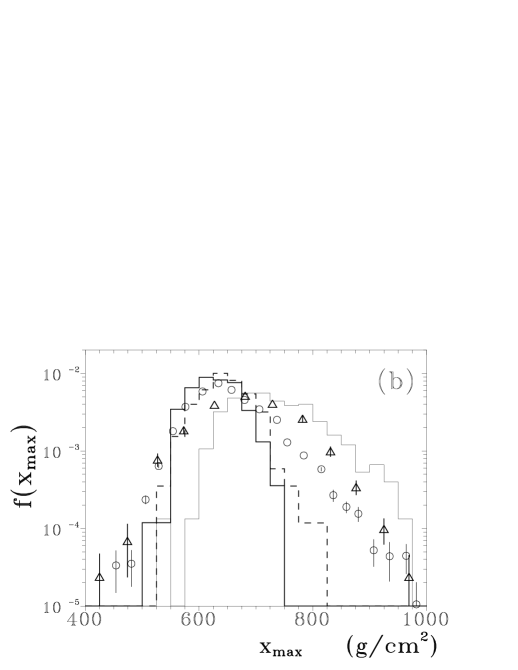
FIG. 5.: Distributions of depths of shower maximum calculated using the GMC model for showers of energies from 10¹⁷ eV to 3$\times$10¹⁷ eV (a), 3$\times$10¹⁷ eV to 10¹⁸ eV (b), 10¹⁸ eV to 3$\times$10¹⁸ eV (c), and 3$\times$10¹⁸ eV to 10¹⁹ eV (d), respectively, for protons (thin histogram) and iron (thick histograms). For the iron primaries the dashed line represents the model without second step cascading process while the solid one is obtained with this process taken into account. The circles represents the Fly’s Eye data from [21]. The Yakutsk data (triangles) from Ref.[22] for showers with average energy of 5$\times$10¹⁷ eV and 5$\times$10¹⁸ eV are given in (b) and (d).

REFERENCES

- [1] T. Wibig, Phys. Rev. D 56, 4350 (1997).
- [2] T. Wibig and D. Sobczyńska, Phys. Rev. D 49, 2268 (1994); D. Sobczyńska and T. Wibig , Izv. Acad. Nauk Fiz. 58, 26 (1994); T. Wibig and D. Sobczyńska, Izv. Acad. Nauk Fiz. 58, 29 (1994); T. Wibig and D. Sobczyńska, Phys. Rev. D 50, 5657 (1994).
- [3] T. Wibig, J. Phys. G 24, 567 (1998).
- [4] B. Anderson, G. Gustafson and H. Pi, Z. Phys. C 50, 405 (1991).
- [5] G. Battistoni, C. Forti and J. Ranft, Astropart. Phys. 3, 157 (1995); A. Ferrari, J. Ranft, S. Roesler and P. R. Sala, Z. Phys. C 70, 413 (1996); ibid. 71, 75 (1996).
- [6] A. Capella, C Pajeras and A. V. Ramallo, Nucl. Phys. B 241, 75 (1984)
- [7] A. Capella, J. Kwiecinski and J. Tran Thanh Van, Phys. Lett. B 108, 347 (1982); A. Kaidalov, Nucl. Phys. A525, 39c (1991). G. Gustafson, ” New Results in the Fritiof Model and collective effects in nuclear collisions”, Lund University Report No. LUTP 92–26 1992 (unpublished).
- [8] T. Wibig and D. Sobczyńska, Phys. Rev D 48, 3110 (1993).
- [9] J. N. Capdevielle, in Proceedings of the 23rd International Cosmic Ray Conference, University of Calgary Publ., Calgary, Canada, 1993, Vol. 4, p. 52.
- [10] R. M. Baltrusaitis et al., Nucl. Instr. Meth. A 240, 410 (1985); G. L. Cassiday, Ann. Rev. Nucl. Part. Sci. 35, 321 (1985).
- [11] G. L. Cassiday et al., Astrophys. J. 356, 669 (1990).
- [12] T. K. Gaisser et al., Phys. Rev D 47, 1919 (1993).
- [13] N. N. Kapeilovich, N. N. Nikolaev and I. K. Potashnikova, Phys. Rev. D 39, 769 (1989).
- [14] D. J. Bird et al., Phys. Rev. Lett. 71, 3401 (1993).
- [15] D. J. Bird et al., Astrophys. J. 424, 491 (1994).
- [16] M. N. Dyakonov et al., in Proceedings of the 23rd Intermational Cosmic Ray Conference, University of Calgary Publ., Calgary, Canada, 1993, Vol. 4, p. 303.
- [17] N. N. Kalmykov, S. S. Ostapchenko and A. I. Pavlov, Inv. Russ Acad. Sci., Ser. Fiz., 58, 21 (1994); N. N. Kalmykov, G. B. Khristiansen, S. S. Ostapchenko and A. I. Pavlov, in Proceedings of the 24rd Intermational Cosmic Ray Conference, University of Roma Publ., Roma, Italy, 1995, Vol. 1, p. 123.
- [18] J. N. Capdevielle et. al, The Karlsruhe Extensive Air Shower Simulation Code CORSIKA, Kernforschungszentrum Karlsruhe Report No. KfK 4998, Forschungszentrum Karlsruhe, Karlsruhe, Germany, 1992.
- [19] W. R. Nelson, H. Hirayama and D. W. O. Rogers, The EGS4 code system, Stanford Linear Accelerator Center Report No. 265, Stanford University, Stanford, California, 1985.
- [20] J. Knapp, D. Heck and G. Schatz, Comparison of Hadronic Interaction Models Used in Air Shower Simulations and of Their Influence on Shower Development and Observables, Forschungszentrum Karlsruhe Report No. FZKA 5828, Forschungszentrum Karlsruhe, Karlsruhe, Germany, 1996.
- [21] D. J. Bird et al., in Proceedings of the 23rd Intermational Cosmic Ray Conference, University of Calgary Publ., Calgary, Canada, 1993, Vol. 2, p. 38.
- [22] M. N. Dyakonov et al., in Proceedings of the 21rd Intermational Cosmic Ray Conference, Adelaide, Australia, 1990, edited by R. J. Protheroe, University of Adelaide Publ., Adelaide, Australia, 1990, Vol. 9, p. 252.
- [23] N. N. Kalmykov and G. B. Khristiansen, J. Phys. G 21, 1279 (1995).
- [24] K. Asakimori et al., in Proceedings of the 23rd Intermational Cosmic Ray Conference, University of Calgary Publ., Calgary, Canada, 1993, Vol. 2, p. 38. calgary Vol. 2 p. 21, 25 (1993).
- [25] V. S. Ptuskin et al., Astron. Astrophys. 268 726, (1993).
- [26] T. Stanev, P. L. Biermann and T. K. Geisser, Astron. Astrophys. 274, 902 (1993).
- [27] K. Boothby et al., Ap. J. 491, L35 (1997).
- [28] J. Cortina et al., Cosmic Ray Spectrum and Chemical Composition in the 300 Tev – 10 PeV Energy Region with the HEGRA Arrays Proc. XVIth Europ. Cosmic Ray Symp., Madrid (1998).