Measurements of electroweak couplings of the $\tau$ lepton at L3

Abstract

We review the current knowledge of the couplings of the $\tau$ lepton to the electroweak gauge bosons, the W, Z and photon, obtained from the full L3 data sample at center-of-mass energies near the Z mass. Measurements of the the effective vector and axial-vector weak neutral couplings of the $\tau$, the Lorentz structure of the weak charged current, and anomalous couplings of the electroweak gauge bosons to the $\tau$ are presented.

I Introduction

The sample of $\tau$ pairs produced in Z decays at LEP has been extensively mined as a source of data for precision electroweak measurements as well as searches for anomalies, including CP violation arising from sources other than the CKM matrix. The short lifetime of the $\tau$ and the rather large catalog of decay modes open up analysis possibilities which are not available for the other leptons at LEP energies. In this note, we survey the measurements of $\tau$ couplings to the Z, the W, and the photon carried out using about $150~{}pb^{-1}$ of data collected near the Z peak by the L3 detector from 1991–1995.

II $\tau$–Z couplings

Measurements of the vector and axial-vector coupling constants of the $\tau$ provide a crucial test of the hypothesis of lepton universality, and, if universality holds, may be combined with other electroweak data to extract a precise measurement of the weak mixing angle. In addition, new physics, possibly including CP violation, may appear in $Z\tau\tau$ couplings as unexpectedly large values of weak magnetic and electric dipole moments.

A Partial width and forward-backward asymmetry

The partial width and forward-backward asymmetry measurements for $Z\rightarrow\tau\tau$ are described in great detail elsewhere [2], and here we reiterate only a few points. The partial width, $\Gamma_{\tau}$, is related to the effective vector and axial-vector couplings by,

$$\Gamma_{\tau}\propto\mbox{$\mid g_{V}^{\tau}\mid^{2}$}+\mbox{$\mid g_{A}^{\tau}\mid^{2}$}$$ (1)

The forward-backward asymmetry, $A_{FB}$ is defined as,

$$A_{FB}=\frac{\sigma(\cos\theta>0)-\sigma(\cos\theta<0)}{\sigma(\cos\theta>0)+\sigma(\cos\theta<0)}$$ (2)

where $\theta$ is the angle between the $\tau^{-}$ and beam electron. This asymmetry is related to the coupling constants by $A_{FB}\simeq{\cal A}_{\tau}{\cal A}_{e}$, where the polarization parameter ${\cal A}_{\ell}$ is defined by,

$${\cal A}_{\ell}=\frac{2Re(\mbox{$g_{V}^{\ell}$}\mbox{$g_{A}^{\ell}$}^{*})}{(\mbox{$\mid g_{V}^{\ell}\mid^{2}$}+\mbox{$\mid g_{A}^{\ell}\mid^{2}$})}$$ (3)

where $\ell$ is an electron or $\tau$.

Measurements of these quantities are combined with the $\tau$ longitudinal polarization measurement described below to determine $\mbox{$g_{V}^{\tau}$}_{\tau}$ and $\mbox{$g_{A}^{\tau}$}_{\tau}$.

B $\tau$ longitudinal polarization and combined measurement of $g_{V}^{\tau}$ and $g_{A}^{\tau}$

The longitudinal, transverse, and normal spin components of the $\tau$, $S_{L},S_{T}$ and $S_{N}$ respectively, are illustrated in Figure 1.

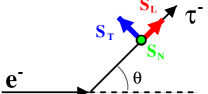
FIG. 1.: Longitudinal, transverse, and normal spin components of the $\tau$.

The $\tau$ longitudinal polarization, ${\cal P}_{\tau}$, is defined by,

$${\cal P_{\tau}}=\frac{\sigma(\mbox{$s_{L}^{\tau^{-}}$}=+1)-\sigma(\mbox{$s_{L}^{\tau^{-}}$}=-1)}{\sigma(\mbox{$s_{L}^{\tau^{-}}$}=+1)+\sigma(\mbox{$s_{L}^{\tau^{-}}$}=-1)}.$$ (4)

In the Standard Model (SM), ${\cal P}_{\tau}$ is non-zero because of parity violation in the weak neutral current. It is most interesting to measure this quantity as a function of the $\tau$ production polar angle, in which case it is related to the coupling constants by [3],

$${\cal P}_{\tau}(\cos\theta)=-\frac{{\cal A}_{\tau}(1+\cos^{2}\theta)+2{\cal A}_{e}\cos\theta}{(1+\cos^{2}\theta)+2{\cal A}_{e}{\cal A}_{\tau}\cos\theta}$$ (5)

where the polarization parameters, ${\cal A}_{\tau}$ and ${\cal A}_{e}$, are defined in equation 3. Thus from this single measurement it is possible to determine almost independently the couplings of the Z to both the $\tau$ and the electron. Also note that the polarization parameters contain products of $g_{V}^{\tau}$ and $g_{A}^{\tau}$, which means that, in contrast to the measurement of $\Gamma_{\tau}$ and $A_{FB}$, this measurement is sensitive to the relative sign of these coupling constants.

The strategy of the measurement is to use the energy and angular distributions of the decay products to infer the longitudinal polarization based upon the assumption that $\tau$ decays proceed via purely $V-A$ interactions. The L3 analysis [4] employs three complementary approaches. First, a selection of exclusive decays is carried out, where we consider the channels $\tau\rightarrow\ell\nu_{\tau}\nu_{\ell}$ ($\ell=e,\mu$) and $\tau\rightarrow h\nu_{\tau}$ ($h=\pi,\rho,a_{1}$). The polarization for each channel is evaluated independently. Second, an analysis of inclusive hadronic decays is performed which recovers some of the information lost for cases in which exclusive identification in hadronic modes is not successful. Third, the polarization is determined from the acollinearity between decay products for events in which there is at least one $\tau\rightarrow\pi\nu_{\tau}$ decay. Results from the three methods are combined accounting for the correlations among them.

Figure 2 shows the final measured ${\cal P}_{\tau}(\cos\theta)$, corrected for QED bremsstrahlung, $\gamma$ exchange and $\gamma$–Z interference, together with the best fit of equation 5. The ratios of the effective vector and axial-vector couplings extracted from this measurement are $\mbox{$g_{V}^{\tau}$}/\mbox{$g_{A}^{\tau}$}=0.0742\pm 0.0055$ and $\mbox{$g_{V}^{e}$}/\mbox{$g_{A}^{e}$}=0.0845\pm 0.0067$. This is consistent with lepton universality.

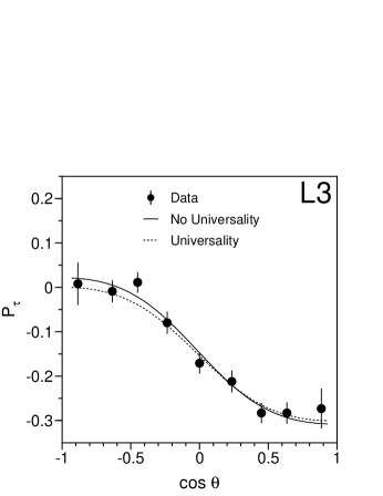
FIG. 2.: $\tau$ polarization together with fits to equation 5.

Assuming universality and combining the longitudinal polarization results with the couplings determined from $\Gamma_{\tau}$ and $A_{FB}$ yields the following preliminary results [5]:

$$g_{V}^{\tau} = -0.0394\pm 0.0032$$

$$g_{A}^{\tau} = -0.5015\pm 0.0019$$

C Transverse-transverse and transverse-normal spin correlations

Correlations between transverse and normal spin components of the two $\tau$’s in a $Z\rightarrow\tau\tau$ event are also sensitive to $\tau$–Z couplings. In terms of the spin components depicted in figure 1, transverse-transverse and transverse-normal spin correlations are written,

$$C_{TT} \propto \frac{\sigma(\mbox{$s_{T}^{\tau^{-}}$}\mbox{$s_{T}^{\tau^{+}}$}=+1)-\sigma(\mbox{$s_{T}^{\tau^{-}}$}\mbox{$s_{T}^{\tau^{+}}$}=-1)}{\sigma(\mbox{$s_{T}^{\tau^{-}}$}\mbox{$s_{T}^{\tau^{+}}$}=+1)+\sigma(\mbox{$s_{T}^{\tau^{-}}$}\mbox{$s_{T}^{\tau^{+}}$}=-1)}$$ (6)

$$C_{TN} \propto \frac{\sigma(\mbox{$s_{T}^{\tau^{-}}$}\mbox{$s_{N}^{\tau^{+}}$}=+1)-\sigma(\mbox{$s_{T}^{\tau^{-}}$}\mbox{$s_{N}^{\tau^{+}}$}=-1)}{\sigma(\mbox{$s_{T}^{\tau^{-}}$}\mbox{$s_{N}^{\tau^{+}}$}=+1)+\sigma(\mbox{$s_{T}^{\tau^{-}}$}\mbox{$s_{N}^{\tau^{+}}$}=-1)}$$ (7)

These are related to the coupling constants by [6],

$$C_{TT} = \frac{\mbox{$\mid g_{A}^{\tau}\mid^{2}$}-\mbox{$\mid g_{V}^{\tau}\mid^{2}$}}{\mbox{$\mid g_{A}^{\tau}\mid^{2}$}+\mbox{$\mid g_{V}^{\tau}\mid^{2}$}}$$ (8)

$$C_{TN} = -\frac{2Im(\mbox{$g_{V}^{\tau}$}\mbox{$g_{A}^{\tau}$}^{*})}{\mbox{$\mid g_{A}^{\tau}\mid^{2}$}+\mbox{$\mid g_{V}^{\tau}\mid^{2}$}}+(\gamma-\mathrm{Z}~{}~{}{\mathrm{I}nterference~{}~{}terms})$$ (9)

Although measurements of these quantities do not add much to the overall precision with which $g_{V}^{\tau}$ and $g_{A}^{\tau}$ are determined, they are interesting for other reasons. Unlike other observables discussed so far, $C_{TT}$ is not symmetric under the interchange of $g_{V}^{\tau}$ and $g_{A}^{\tau}$, and is thus an on-peak observable which can be used to break this ambiguity. $C_{TN}$ is of particular interest as it is both P and T-odd.

For $\tau$-pair events with exactly two charged particles in the final state, $C_{TT}$ and $C_{TN}$ can be measured using azimuthal asymmetries in the coordinate system of figure 3.

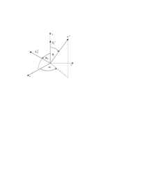
FIG. 3.: Coordinate system used to measure spin correlations. The $z$ axis is defined by the direction of the negatively charged $\tau$ decay product, the $x-z$ plane is defined by the directions of the two charged decay products. $\omega$ is the azimuthal angle of the beam electron.

The differential cross-section in terms of $\omega$ contains pieces which depend on $C_{TT}$ and $C_{TN}$:

$$\frac{d\sigma}{d\omega}=A+B\left({C_{TT}}\cos 2\omega+{C_{TN}}\sin 2\omega\right)$$ (10)

where $A$ and $B$ are constants.

Asymmetries constructed from this distribution yield the preliminary results [7] $C_{TT}=0.99\pm 0.24\pm 0.08$ and $C_{TN}=0.15\pm 0.24\pm 0.07$. These are consistent with SM predictions [6] of $C_{TT}\sim 0.99$ and $C_{TN}=-0.01$.

D Weak dipole moments

Weak dipole moments of the $\tau$ may be introduced through an effective Lagrangian which contains electric- and magnetic-type pieces,

$${\cal L}^{eff}_{\mathrm{int}}=\frac{-i}{2}\frac{e{F_{3}^{w}(q^{2})}}{2m_{\tau}}\overline{\psi}\sigma^{\mu\nu}\gamma_{5}\psi Z_{\mu\nu}+\frac{1}{2}\frac{e{F_{2}^{w}(q^{2})}}{2m_{\tau}}\overline{\psi}\sigma^{\mu\nu}\psi Z_{\mu\nu}$$ (11)

where $Z_{\mu\nu}=\partial_{\mu}Z_{\nu}-\partial_{\nu}Z_{\mu}$. The weak magnetic and weak electric dipole moments are defined in terms of these form factors as $a_{\tau}^{w}=F_{2}^{w}(q^{2}=m_{Z}^{2})$ and $d_{\tau}^{w}=eF_{3}^{w}(q^{2}=m_{Z}^{2})/2m_{\tau}$, respectively. In the SM, these moments are zero at tree-level but acquire small contributions from loops, leading to the following predictions [8, 9]:

$$a_{\tau}^{w} = -(2.10+0.61i)\times 10^{-6}$$

$$d_{\tau}^{w} \sim 3\times 10^{-37}e\cdot\mathrm{cm}$$

Such tiny values are beyond the experimental reach of LEP, but observation of a significant non-zero value would unambiguously signal new physics. In particular, a non-zero value of $d_{\tau}^{w}$ would imply CP violation in the decay $Z\rightarrow\tau\tau$.

The L3 measurement of $a_{\tau}^{w}$ and $d_{\tau}^{w}$ exploits the dependence of the transverse and normal polarizations of single $\tau$’s on these moments. These polarization components can be determined from asymmetries in the azimuthal angle, $\phi_{h}^{-}$, defined in figure 4. This analysis is limited to decays of the type $e^{+}e^{-}\rightarrow\tau^{+}\tau^{-}\rightarrow h^{+}\overline{\nu}_{\tau}h^{-}\nu_{\tau}$, were $h^{\pm}$ is a charged hadron, as it is necessary to reconstruct the $\tau$ flight direction, a task that is not possible if there are more than two neutrinos in the event.

FIG. 4.: Coordinate system used to define azimuthal asymmetries which are sensitive to weak dipole moments. Ths $z$ axis is defined by the $\tau^{-}$ flight direction, and the $x-z$ plane is defined by the $\tau^{-}$ flight direction and the direction of the beam electron.

In this coordinate system, the differential cross section takes the form [9, 10],

$$\frac{d\sigma}{d(\cos\theta_{\tau^{\pm}})d\phi_{h^{\pm}}}={\mathrm{S}M~{}part}+X\cos\phi_{h^{\pm}}+Y\sin\phi_{h^{\pm}}$$ (12)

where $X=X(\theta_{\tau^{\pm}},F_{2}^{w})$ and $Y=Y(\theta_{\tau^{\pm}},F_{3}^{w})$. Equation 12 is then used to define asymmetries from which $a_{\tau}^{w}$ and $d_{\tau}^{w}$ can be calculated.

The final results of the measurement are [11]:

$$Re(a_{\tau}^{w}) = (0.0\pm 1.6\pm 2.3)\times 10^{-3}$$

$$Im(a_{\tau}^{w}) = (-1.0\pm 2.6\pm 5.3)\times 10^{-3}$$

$$Re(d_{\tau}^{w}) = (-0.44\pm 0.88\pm 1.33)\times 10^{-17}e\cdot\mathrm{cm}$$

This is the first measurement of $a_{\tau}^{w}$.

III Lorentz structure of the charged current

In addition to the studies of the weak neutral current just discussed, the Lorentz structure of the charged current in $\tau$ decays can also be studied. Leptonic decays can be described by a general derivative-free four-fermion contact interaction [12, 13],

$${\cal M}=\frac{4G_{F}}{\sqrt{2}}\sum_{\stackrel{{\scriptstyle\scriptstyle\gamma=S,\,V,\,T}}{{\lambda,\,\iota=R,\,L}}}g_{\lambda\iota}^{\gamma}<\overline{l}_{\lambda}|\Gamma^{\gamma}|(\nu_{l})_{n}><(\overline{\nu}_{\tau})_{m}|\Gamma_{\gamma}|\tau_{\iota}>.$$ (13)

where $\iota$ and $\lambda$ label the helicity of the $\tau$ and the final–state charged lepton respectively and $\gamma$ labels the current as scalar, vector or tensor. In the SM, the coefficient $g_{LL}^{V}=1$ and all the other coefficients are zero. The 10 possible (complex) constants $g_{\lambda\iota}^{\gamma}$ are conventionally expressed in terms of Michel parameters [13], of which 4 are accessible through measurements of the leptonic decay spectra. Specifically, the four Michel parameters $\rho,\eta,\xi$ and $\xi\delta$ enter the decay spectrum as follows [14]:

$$\frac{1}{\Gamma}\frac{d\Gamma}{dx_{l}} = {H_{0}^{l}(x_{l})}-{{\cal P}_{\tau}}{H_{1}^{l}(x_{l})}$$ (14)

$$= {h_{0}^{l}(x_{l})+\eta h_{\eta}^{l}(x_{l})+\rho h_{\rho}^{l}(x_{l})}-{{\cal P}_{\tau}}[{\xi h_{\xi}^{l}(x_{l})+\xi\delta h_{\xi\delta}^{l}(x_{l})}]$$ (15)

where $x_{l}$ is the lepton energy normalized to the beam energy and ${\cal P}_{\tau}$ is the $\tau$ longitudinal polarization, and the $h$’s are kinematic factors.

Semileptonic decays can be described in a similar way:

$$\frac{1}{\Gamma}\frac{d\Gamma}{dx_{h}} = {H_{0}^{h}(x_{h})}-{{\cal P}_{\tau}}{H_{1}^{h}(x_{h})}$$ (16)

$$= {h_{0}^{h}(x_{h})}-{{\cal P}_{\tau}}{\xi_{h}h_{1}^{h}(x_{h})}$$ (17)

where in the case of $\tau\rightarrow\rho\nu_{\tau}$, $x_{h}$ is a quantity constructed from the energies and angles of the $\rho\rightarrow\pi\pi^{0}$ decay products which maximizes sensitivity to ${\cal P}_{\tau}$ [15]. The parameter $\xi_{h}$ is the average helicity of the $\tau$ neutrino.

From equations 14 and 16 it is apparent that $\xi$, $\xi_{h}$ and $\xi\delta$ cannot be determined independently from ${\cal P}_{\tau}$ using just these distributions. However, if one assumes only $V$ and $A$ interactions in $\tau$ pair production, then the helicities of the two $\tau$’s are nearly $100\%$ anticorrelated. This can be exploited to write a double decay distribution in which all of these Michel parameters are disentangled from ${\cal P}_{\tau}$:

$$\frac{1}{\Gamma}\frac{d^{2}\Gamma}{dx_{A}dx_{B}} = H_{0}^{(A)}(x_{A})H_{0}^{(B)}(x_{B})+H_{1}^{(A)}(x_{A})H_{1}^{(B)}(x_{B})$$ (19)

$$\mbox{}-{\mbox{${\cal P}_{\tau}$}}\ \left[H_{1}^{(A)}(x_{A})H_{0}^{(B)}(x_{B})+H_{0}^{(A)}(x_{A})H_{1}^{(B)}(x_{B})\right]$$

The strategy adopted for the L3 measurement is thus to carry out common fit to all the leptonic and semileptonic channels, including both joint distributions and single distributions in cases where one $\tau$ decay is not identified. The Michel parameters and $\tau$ polarization are extracted simultaneously from this fit, with the results [16] shown in Table I. These results support the hypothesis of $V-A$ structure of the weak charged current in $\tau$ decays.

TABLE I.: Results of Michel parameter measurements and $\tau$ polarization together with parameters expected for purely $V-A$ interactions.

Parameter	Measured Value	SM expectation
$\rho$	0.762 $\pm$ 0.035	0.75
$\eta$	0.27 $\pm$ 0.14	0
$\xi$	0.70 $\pm$ 0.16	1
$\xi\delta$	0.70 $\pm$ 0.11	0.75
$\xi_{h}$	-1.032 $\pm$ 0.031	-1
${\cal P}_{\tau}$	-0.164 $\pm$ 0.016

IV Anomalous electromagnetic moments of the $\tau$

Finally we turn to $\tau-\gamma$ couplings and in particular what can be learned from studying radiative $\tau$ pair production at LEP. A $\tau$ may couple to a photon through its charge, magnetic dipole moment or electric dipole moment . These couplings can be parametrized by a matrix element in which the usual $\gamma^{\mu}$ describing the current is replaced by a more general Lorentz-invariant form:

$$\Gamma^{\mu}=F_{1}(q^{2})\gamma^{\mu}+\frac{iF_{2}(q^{2})}{2m_{\tau}}\sigma^{\mu\nu}q_{\nu}-F_{3}(q^{2})\sigma^{\mu\nu}\gamma^{5}q_{\nu}$$ (20)

If $q^{2}=0$ and if the $\tau$ is real on both sides of the $\tau\tau\gamma$ vertex, the form factors $F_{i}(q^{2})$ have the following interpretations: $F_{1}(0)\equiv Q_{\tau}$ is the electric charge; $F_{2}(0)\equiv a_{\tau}$ is the anomalous magnetic moment ($a_{\tau}\equiv(g_{\tau}-2)/2$); and $F_{3}(0)\equiv d_{\tau}/Q_{\tau}$, where $d_{\tau}$ is the electric dipole moment. In the SM $a_{\tau}$ is non-zero due to loops and is calculated to be $a_{\tau_{SM}}=0.001\,177\,3(3)$ [17]. Although this value turns out to be beyond the current experimental reach using radiative $\tau$ decays, phenomena such as compositeness or leptoquarks [18] could influence values of anomalous moments. The measurement of $d_{\tau}$ is also quite interesting as a non-zero value is forbidden by both $P$ and $T$ invariance.

In order to assess the effects of anomalous electromagnetic moments on radiative $\tau$ pair production, a tree level calculation of the squared matrix element for the process $e^{+}e^{-}\rightarrow\tau^{+}\tau^{-}\gamma$ has been carried out [19] which includes the contributions from all the form factors in equation 20, Z and $\gamma$ exchange, $\gamma$-Z interference and the interference between SM and anomalous amplitudes. Large values of $F_{2}(0)$ or $F_{3}(0)$ turn out to increase the overall rate of $\tau\tau\gamma$ events and in particular enhance the production of high energy, isolated photons.

Selection of $\tau\tau\gamma$ events is relatively straightforward, though managing the background requires care [20]. Figure 5 shows the energy and angular distributions of the selected events together with the Monte Carlo predictions for $F_{2}(0)=0$ and $F_{2}(0)=0.1$.

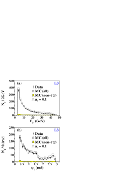
FIG. 5.: Number of photon candidates $(N_{\gamma})$ as a function of a) photon energy and b) opening angle between the $\gamma$ and the nearest $\tau$. The dashed line shows what one would expect to observe for $a_{\tau}=0.1$.

To extract $F_{2}(0)$ and $F_{3}(0)$ from the data, a two-dimensional fit is performed to the photon energy and the opening angle between the photon and the nearest $\tau$. In order to exploit the sensitivity of the overall rate to the anomalous moments, the normalization is fixed to the integrated luminosity. The results are consistent with SM expectations, and the following 95% C.L. limits are set [20]:

$$-0.052< F_{2}(0) <0.058$$

$$(-3.1< F_{3}(0) <3.1)\times 10^{-16}\mathrm{e}\cdot\mathrm{cm}$$

V Conclusions

The plethora of $\tau$ physics analysis carried out using the LEP data sample includes important precision measurements of weak neutral and charged current couplings and searches for new phenomena. The L3 collaboration has finalized or nearly finalized most of its analyses of $\tau$ couplings. The results show no significant deviation from the hypothesis of lepton universality or the $V-A$ structure of the charged current. The spin analysis of the $\tau$ has been recently extended beyond measurement of the longitudinal polarization to include transverse and normal spin correlations. Searches for anomalous couplings did not turn up anything unexpected, but have provided measurements of quantities for which there was little or no previous information, including the first measurement of the $\tau$ weak magnetic dipole moment and the most stringent limits on the anomalous electromagnetic moments.

REFERENCES

- [1]
-
[2]
LEP electroweak working group and SLD heavy flavor group,
“Combination of Preliminary Electroweak Measurements and Constraints on the Standard Model.”
CERN-PPE/97A.
L3 Collab. paper in preparation. - [3] S. Jadach, Z. Wa̧s et al., in ‘Z Physics at LEP 1’, CERN Report CERN 89-08, eds. G Altarelli, R. Kleiss and C Verzegnassi (CERN, Geneva, 1989) Vol. 11, p. 235.
- [4] L3 Collab., M. Acciarri et al., Phys. Lett. B429, 387 (1998).
- [5] J. Mnich, private communication.
-
[6]
J. Bernabéu, N. Rius and A. Pich, Phys. Lett. B257, 219 (1991);
J. Bernabéu, N. Rius, Phys. Lett. B232, 127 (1989). -
[7]
R. Völkert, Ph.D. Thesis, Deutsches Elektronen-Synchrotron DESY,
Institut für Hochenergiephysic ifH, Zeuthen, Germany (1997).
A. Zalite, private communication. - [8] J. Bernabéu, G.A. González-Sprinberg, M. Tung, J. Vidal, Nucl. Phys. B436, 474 (1995).
- [9] W. Hollik, J.I. Illana, C. Schappacher, D. Stöckinger, S. Rigolin, Preprint KA-TP-10-1998.
- [10] J. Bernabéu, G.A. González-Sprinberg, J. Vidal, Phys. Lett. B326, 168 (1994).
- [11] L3 Collab., M. Acciarri et al., Phys. Lett.B426, 207 (1998).
- [12] F. Scheck, “Leptons, Hadrons and Nuclei,” North Holland Physics Publishing, Amsterdam (1983).
- [13] K. Mursula and F. Scheck, Nucl. Phys. B253, 189 (1985).
-
[14]
C. Nelson, Phys. Rev. D40, 123 (1989), erratum Phys. Rev. D41, 2327 (1990);
W. Fetscher, Phys. Rev. D42, 1544 (1990);
R. Alemany et al., Nucl. Phys. B379, 3 (1992). - [15] M. Davier, L. Duflot, F. Le Diberder and A. Rougé, Phys. Lett. B306, 411 (1993).
- [16] L3 Collab., M. Acciarri et al., Phys. Lett. B438, 405 (1998).
-
[17]
M.A. Samuel, G. Li and R. Mendel, Phys. Rev. Lett. 67, 668 (1991),
erratum ibid 69, 995 (1992).;
F. Hamzeh and N.F. Nasrallah, Phys. Lett. B373, 221 (1996). -
[18]
D.J. Silverman, G.L. Shaw, Phys. Rev. D27, 1196 (1983);
J.L. Hewett, T.G. Rizzo, Phys. Rev. D56, 5709 (1997). -
[19]
S.S. Gau, T. Paul, J. Swain, L. Taylor, Nucl. Phys. B523, 439 (1998);
T. Paul and Z. Wa̧s, hep-ph/9801301. - [20] L3 Collab., M. Acciarri et al., Phys. Lett. B434, 169 (1998).