2-Loop Supersymmetric Renormalisation Group Equations Including R-Parity Violation and Aspects of Unification

Abstract

We present the complete 2-loop renormalisation group equations of the superpotential parameters for the supersymmetric standard model including the full set of $R$-parity violating couplings. We use these equations to do a study of (a) gauge coupling unification, (b) bottom-tau unification, (c) the fixed-point structure of the top quark Yukawa coupling, and (d) two-loop bounds from perturbative unification. For large values of the R-parity violating coupling, the value of $\alpha_{S}(M_{Z})$ predicted from unification can be reduced by 5$\%$ with respect to the R-parity conserving case, bringing it to within 2$\sigma$ of the observed value. Bottom-tau Yukawa unification becomes potentially valid for any value of $\tan\beta\sim 2-50$. The prediction of the top Yukawa coupling from the low $\tan\beta$, infra-red quasi fixed point can be lowered by up to $10\%$, raising $\tan\beta$ up to a maximum of 5 and relaxing experimental constraints upon the quasi-fixed point scenario. For heavy scalar fermion masses ${\mathcal{O}}(1\mbox{~{}TeV})$ the limits on the higher family $\Delta L\not=0$ operators from perturbative unification are competitive with the indirect laboratory bounds. We calculate the dependence of these bounds upon $\tan\beta$.

1 Introduction

The first grand unified theory (GUT), of the electroweak and the strong interactions was non-supersymmetric and the unification scale was of order $M_{X}=10^{15}\mbox{~{}GeV}$ [1]. In order to connect the GUT predictions at $M_{X}$ with observations at presently accessible energies, the renormalisation group evolution of the relevant parameters must be taken into account [2]. Postulating unification of the gauge couplings at a high scale leads after renormalisation to one low-energy prediction, e.g. the electroweak mixing angle $\sin^{2}\theta_{W}$. In 1987, it was first found that in supersymmetry the prediction for $\sin^{2}\theta_{W}$ is in agreement with the data, while in the Standard Model it is not [3, 4]. This was spectacularly confirmed in 1990 with the precise LEP1 measurements of the gauge couplings constants [5, 6]. This is the most compelling “experimental” indication for supersymmetry and has lead to a flourish of activity on unification and supersymmetry [7, 5, 8]. These studies focused on the minimal supersymmetric Standard Model (MSSM) which is minimal in particle content and couplings and conserves the discrete and multiplicative symmetry R-parity [9]

$$R_{p}=(-)^{3B+L+2S}.$$ (1.1)

We refer to this model as the $R_{p}$-MSSM, i.e. the $R_{p}$ conserving MSSM.

If we require a supersymmetric Standard Model which is only minimal in particle content the superpotential is modified to allow for additional R-parity violating ($\not\!\!R_{p}$) interactions which are given in full below in Eq.(2.3). The superpotential includes terms which violate baryon number and separate terms violating lepton-number. In order to avoid rapid proton decay either baryon number or lepton number must be conserved but not necessarily both. We refer to a model which violates just one of these symmetries as an $\not\!\!R_{p}$-MSSM, [10]. Symmetries which can achieve this are for example baryon parity and lepton parity [11, 12]

$$B_{p}=(-)^{3B+2S},\quad L_{p}=(-)^{L+2S}.$$ (1.2)

Thus, both the $R_{p}$-MSSM and the $\not\!\!R_{p}$-MSSM require a discrete symmetry beyond $G_{SM}$ and are theoretically equally well motivated [10].

1.1 R-parity Violation and Grand Unification

Given the intense study of unification in the $R_{p}$-MSSM it is the purpose of this paper to study the gauge coupling unification in the $\not\!\!R_{p}$-MSSM. At first sight, it might seem unnatural to study unification within the $\not\!\!R_{p}$-MSSM, since $\not\!\!R_{p}$ is not obtained in the simplest GUT models. In $SU(5)$ for example, the dimension-four R-parity violating interactions are given by the operator

$${\overline{\psi}_{i}}{\overline{\psi}_{j}}{\chi_{k}},$$ (1.3)

where $i,j,k=1,2,3$ are generation indices, and ${\overline{\psi}_{i}},\;{\chi_{k}}$ are the ${\overline{\bf 5}}$, and $\bf 10$ representations of $SU(5)$ respectively. The operator (1.3) contains all the cubic terms of Eq.(2.3), i.e. both the baryon- and lepton-number violating interactions. This leads to unacceptably rapid proton decay or unnaturally small couplings ($\sim 10^{-13}$) and thus must not be present. In $SO(10)$ and in $E_{6}$ grand unification the dimension-four R-parity violating interactions are directly prohibited by gauge invariance.

It seems R-parity violation and GUTs are incompatible. The reason is that any R-parity violating symmetry which is consistent with the bounds on proton decay, such as baryon parity and lepton parity in Eq.(1.2), assigns quarks and leptons different quantum numbers. But in GUTs quarks and leptons are in common multiplets and thus must have the same non-$SU(5)$ quantum numbers. This contradiction is resolved once the GUT symmetry is broken, i.e. for energy scales below $M_{GUT}$. Once the $SU(5)$ symmetry is broken, R-parity violating terms can be generated which are consistent with proton decay.

In general, we do not expect a GUT to be the final theory, it leaves many of the same questions unanswered as in the Standard Model. For example GUTs do not include gravity and therefore it should be an effective theory embedded in a more fundamental one, such as M-theory. This more fundamental theory will lead to a set of non-renormalisable operators at the GUT scale such as [13]

$$\frac{k}{M_{X}}{\overline{\psi}_{i}}{\overline{\psi}_{j}}{\chi_{k}}\Sigma.$$ (1.4)

This operator is suppressed by a mass scale $M_{X}\stackrel{{\scriptstyle>}}{{\sim}}M_{GUT}$. Here, $\Sigma$ is a scalar field in the adjoint representation of $SU(5)$ and $k$ is a dimensionless coupling constant. ${\overline{\psi}_{i}}$, ${\overline{\psi}_{j}}$, ${\chi_{k}}$ and $\Sigma$ can be combined to $SU(5)$ invariants in several ways. When $\Sigma$ receives a non-zero vacuum expectation value $SU(5)$ is broken and the operators in Eq.(1.4) can generate a subset of the $\not\!\!R_{p}$ interactions in the superpotential (2.3), which are consistent with bounds on proton decay [13]. Models of this nature have been constructed for the gauge groups $SU(5)$ [11, 13, 14, 15], $SU(5)\times U(1)$ [16, 13, 14] and $SO(10)$ [13].

Below the $SU(5)$ breaking-scale the operators (1.4) are effectively dimension-four operators. Their dimensionless coupling constant $k<\!\Sigma\!>/M_{X}$ will run, i.e. it will be renormalised and it will contribute to the running of the other couplings in the theory. Thus even though at first sight GUTs and R-parity violation seem inconsistent, this is not the case. Unless prohibited by a special symmetry, we expect to have R-parity violation via non-renormalisable operators in any GUT. At low-energy, this will manifest itself in (effective) tri-linear R-parity violating contributions to the superpotential. Above the GUT scale we will have an $SU(5)$ symmetric theory with for example one unified gauge coupling constant.

1.2 Unification and Fermion Masses

One particular aspect of unification we will focus on below is the GUT prediction $m_{b}(M_{U})=m_{\tau}(M_{U})$ which has been very successful [17, 18, 19]. We shall study the effect of R-parity violation on this prediction. If there are no non-renormalisable operators leading to effective fermion masses below $M_{GUT}$, or if these operators are highly suppressed then we expect the Yukawa unification to still hold in the presence of R-parity violation. This can typically be achieved by a discrete symmetry but should be incorporated in a general theory of fermion masses (or Yukawa couplings). If the non-renormalisable terms have the form

$$W=h_{ij}^{u}(\Sigma)\chi_{i}\chi_{j}h_{u}+h_{ij}^{e,d}(\Sigma)\chi_{i}{\overline{\psi}}_{j}h_{d},$$ (1.5)

the mass predictions are maintained. Here $h_{u},\,h_{d}$ are the $SU(5)$ $5$ and $\overline{5}$ Higgs superfields, respectively. $h_{ij}^{u},\,h_{ij}^{e,d}$ are general functions of the adjoint Higgs field. When $SU(5)$ is broken and $<\!\Sigma\!>\not=0$, the usual mass terms are generated.

In the MSSM, if one requires the Yukawa couplings to unify this greatly reduces the allowed region of the (supersymmetric) parameters. In particular one obtains a strict relation between the running top mass $m_{t}(m_{t})$ and the ratio of the vacuum expectation values (vevs) of the two Higgs doublets, $\tan\beta$ [7, 20]. Given the observed top quark mass [21] this results in a prediction for $\tan\beta\sim 1-3$ or $\tan\beta\sim 55$. Does this prediction still hold when allowing for R-parity violation? In Ref. [22], by allowing only the bi-linear lepton number violating terms, it is shown that bottom-tau Yukawa unification can occur for any value of $\tan\beta$. The bi-linear term induces a tau-sneutrino vev, which introduces an additional parameter into the relation between $\lambda_{t}$ and $m_{t}$, as compared to the MSSM. Bottom-tau Yukawa unification is then obtained by varying the stau vev, and therefore $\lambda_{t}$ (and hence $\tan\beta$). Here, we will focus on the effect of the tri-linear $\not\!\!R_{p}$ terms upon the bottom-tau unification scenario. The third generation $\not\!\!R_{p}$-couplings enter the evolution of $m_{t},\,m_{b}$, and $m_{\tau}$ at one loop and can thus have a large effect. Thus if we allow for $\not\!\!R_{p}$ we expect the strict predictions of the MSSM to be modified. In Section 6 we shall analyse this effect and show that bottom-tau Yukawa unification becomes viable for any value of $\tan\beta$, each one corresponding to a particular value of an $\not\!\!R_{p}$ coupling.

There has been much work to predict the fermion masses at the weak scale from a simple symmetry structure at the unification scale [18, 23]. It is possible that the fermion mass structure is determined by a broken symmetry [24] where only the top-quark Yukawa coupling is allowed by the symmetry at tree-level. Its value is put in by hand and is presumably of order one. The other couplings are then determined dynamically through the symmetry breaking model. Given such a model, we would then still require a prediction for the top-quark Yukawa coupling. An intriguing possibility is that this Yukawa coupling is given by an infra-red (quasi) fixed point [25]. The low-energy value then depends only very weakly on the high-energy initial value; the exact opposite of a fine-tuning problem. In supersymmetric GUTs with bottom-tau unification one typically requires large values of $\lambda_{t}\sim 1$ close to the IR quasi fixed-point. This has been studied in detail in Refs.[7, 20, 18, 26, 27]. We investigate the effect of the $\not\!\!R_{p}$-couplings on the fixed point in Section 7. Similar to the case of bottom-tau unification in section 6 we find fixed-point structures for the top Yukawa coupling for any value of $\tan\beta$, although the focussing behaviour can be weakened depending upon the particular coupling introduced.

1.3 Present Status

There have been several previous studies of the renormalisation group equations (RGEs) of the $\not\!\!R_{p}$-Yukawa couplings [28, 29, 30, 31, 32], which have all been at the one-loop level. The main point of this paper is that we present the two-loop equations for the first time. In [30, 29] the unitarity bounds on the couplings were determined at one-loop. These are still the best bounds on some of the baryon-number violating couplings. Below we update these bounds using the two-loop renormalisation group equations (RGEs). In [28] the complete one-loop RGEs for the dimensionless couplings were first presented and the fixed point structure was studied. We differ slightly in philosophy by also considering the Yukawa unification scenario as discussed above and considering the fixed point structure at two-loop in the RGEs. In [32] the full one-loop RGEs including the soft breaking terms were presented. These were used to study the bounds from flavour changing neutral currents. We do not here consider the RGEs for the soft breaking terms and this work is thus complimentary to ours. Several models have also been constructed implementing one-loop equations including the soft-terms [31]. Since our results are mainly model independent we do not comment on this work here.

The most important effect which enters at two-loop is that the running of the gauge couplings now depends on the $\not\!\!R_{p}$-couplings. One might expect this effect to be small. But for higher generations the bounds on the $\not\!\!R_{p}$-couplings are weak and the couplings can be of order the electromagnetic coupling ($e\approx 0.30$) or more. In addition, most bounds are presented for scalar fermion masses of $100\mbox{~{}GeV}$ and become weaker for higher masses. At present the best 1$\sigma$ empirical bounds for the highest generation couplings and for relevant scalar fermion masses of $1\mbox{~{}TeV}$ are [10, 34]

$$\lambda_{323}<0.6\,\quad\lambda^{\prime}_{333}<2.6\,\quad{\lambda^{\prime\prime}}_{323}<0.43^{*},$$ (1.6)

where the asterisk indicates the bound for a $100\mbox{~{}GeV}$ mass, and does not have a simple analytic description of the scaling with mass. At $1.5\mbox{~{}TeV}$ the bound on $\lambda_{323}$ [35] is almost identical to the perturbative limit obtained below in Section 3. The bound on $\lambda^{\prime}_{333}$ [34] at $1\mbox{~{}TeV}$, is obtained by scaling and as such is meaningless since perturbation theory breaks down below $M_{U}$ for such large values. The appropriate bound is thus the perturbative limit, which we obtain in Section 3. A mass-independent bound on $\lambda^{\prime\prime}_{323}$ was found in ref.[36] from requiring perturbativity up to the scale $M_{U}$. However, we show below that the bound from perturbative unification is dependent upon $\tan\beta$, and we calculate this dependence. We shall thus explore all three couplings to the perturbative limit.

The outline of the paper is as follows. In Section 2 we present the full two-loop renormalisation group equations for the gauge couplings and the superpotential parameters. In Section 3 we present the specific RGEs assuming there is only one $\not\!\!R_{p}$-operator present at a time. In Section 4 we outline the procedure for our numerical analysis. In Section 5 we use the specific equations to study the effects of R-parity violation on the unification of the gauge couplings. We focus on the main predictions of unification: the unification scale, the value of the gauge coupling at the unification scale and the value of the strong coupling at $M_{Z}$. In Section 6 we study the effects of the third generation $\not\!\!R_{p}$-couplings on $b$-$\tau$ unification. In Section 7 we study the Landau poles and the fixed points of the top- and the $\not\!\!R_{p}$-Yukawa couplings. In Section 8 we present our conclusions.

2 Renormalisation Group Equations

The chiral superfields of the $R_{p}$-MSSM and the $\not\!\!R_{p}$-MSSM have the following $G_{SM}=SU(3)_{c}\times SU(2)_{L}\times U(1)_{Y}$ quantum numbers

$$L: (1,2,-\frac{1}{2}),\quad{\bar{E}}: (1,1,1),\qquad\,Q:\,(3,2,\frac{1}{6}),\quad{\bar{U}}:\,(3,1,\frac{2}{3}),$$

$${\bar{D}}: (3,1,-\frac{1}{3}),\quad H_{1}: (1,2,-\frac{1}{2}),\quad H_{2}:\,(1,2,\frac{1}{2}).$$ (2.1)

In the following we shall apply the work of Martin and Vaughn (MV) [37] to the general $\not\!\!R_{p}$-MSSM superpotential. For the generic superpotential, $W$, we closely follow their notation

$$W=Y^{\phi_{\rho}\phi_{\sigma}\phi_{\delta}}\phi_{\rho}\phi_{\sigma}\phi_{\delta}/6,$$ (2.2)

where $\phi_{\rho,\sigma,\delta}$ denote any chiral superfield of the model. The indices ${\rho,\sigma,\delta}$ run over all gauge and flavour components. The $\not\!\!R_{p}$-MSSM superpotential is then given by

$$W = \epsilon_{ab}\left[({{\bf Y}}_{E})_{ij}L_{i}^{a}H_{1}^{b}{\bar{E}}_{j}+({{\bf Y}}_{D})_{ij}Q_{i}^{ax}H_{1}^{b}{\bar{D}}_{jx}+({{\bf Y}}_{U})_{ij}Q_{i}^{ax}H_{2}^{b}{\bar{U}}_{jx}\right]$$ (2.3)

$$+\epsilon_{ab}\left[\frac{1}{2}({{\bf\Large\Lambda}}_{E^{k}})_{ij}L_{i}^{a}L_{j}^{b}{\bar{E}}_{k}+({{\bf\Large\Lambda}}_{D^{k}})_{ij}L_{i}^{a}Q_{j}^{xb}{\bar{D}}_{kx}\right]+\frac{1}{2}\epsilon_{xyz}({{\bf\Large\Lambda}}_{U^{i}})_{jk}{\bar{U}}_{i}^{x}{\bar{D}}_{j}^{y}{\bar{D}}^{z}_{k}$$

$$+\epsilon_{ab}\left[\mu H_{1}^{a}H_{2}^{b}+\kappa^{i}L_{i}^{a}H_{2}^{b}\right].$$

We denote an $SU(3)$ colour index of the fundamental representation by $x,y,z=1,2,3$. The $SU(2)_{L}$ fundamental representation indices are denoted by $a,b,c=1,2$ and the generation indices by $i,j,k=1,2,3$. We have introduced the twelve $3\times 3$ matrices

$${{\bf Y}}_{E},\quad{{\bf Y}}_{D},\quad{{\bf Y}}_{U},\quad{{\bf\Large\Lambda}}_{E^{k}},\quad{{\bf\Large\Lambda}}_{D^{k}},\quad{{\bf\Large\Lambda}}_{U^{i}},$$ (2.4)

for all the Yukawa couplings. This implies the following conventions in the MV notation

$$Y^{L_{i}^{a}Q^{bx}_{j}\bar{D}_{ky}} = Y^{L_{i}^{a}\bar{D}_{ky}Q^{bx}_{j}}=Y^{\bar{D}_{ky}L_{i}^{a}Q^{bx}_{j}}=Y^{Q^{bx}_{j}L_{i}^{a}\bar{D}_{ky}}$$ (2.5)

$$= Y^{Q^{bx}_{j}\bar{D}_{ky}L_{i}^{a}}=Y^{\bar{D}_{ky}Q^{bx}_{j}L_{i}^{a}}=({{\bf\Large\Lambda}}_{D^{k}})_{ij}\epsilon_{ab}\delta^{y}_{x},$$

$$Y^{L_{i}^{a}L_{j}^{b}\bar{E}_{k}} = Y^{L_{i}^{a}\bar{E}_{k}L_{j}^{b}}=Y^{\bar{E}_{k}L_{i}^{a}L_{j}^{b}}=({{\bf\Large\Lambda}}_{E^{k}})_{ij}\epsilon_{ab}=-({{\bf\Large\Lambda}}_{E^{k}})_{ji}\epsilon_{ab},$$ (2.6)

$$Y^{{\bar{U}}_{ix}{\bar{D}}_{jy}{\bar{D}}_{kz}} = Y^{{\bar{D}}_{jy}{\bar{U}}_{ix}{\bar{D}}_{kz}}=Y^{{\bar{D}}_{jy}{\bar{D}}_{kz}{\bar{U}}_{ix}}=\epsilon_{xyz}\left({\bf\Lambda}_{U^{i}}\right)_{jk}=-\epsilon_{xyz}\left({\bf\Lambda}_{U^{i}}\right)_{kj},$$ (2.7)

We denote the $G_{SM}$ gauge couplings by $g_{3}$, $g_{2}$, $g_{1}$. In Appendix A we have collected several useful group theoretical formulas pertaining to $G_{SM}$ and the above field content. Here we mention that for $U(1)_{Y}$ we use the normalisation as in GUTs and thus use $g_{1}=\sqrt{3/5}\,g_{Y}$. More details are given in the appendix. We define our notation for the Yukawa couplings via the superpotential including all $\not\!\!R_{p}$ terms.

We now in turn study the dimensionless couplings and then briefly also discuss the mass terms $\mu,\kappa_{i}$. We do not consider the soft-breaking terms here.

2.1 Gauge Couplings

The renormalisation group equations for the gauge couplings are

$$\frac{d}{dt}g_{a}=\frac{g_{a}^{3}}{16\pi^{2}}B_{a}^{(1)}+\frac{g_{a}^{3}}{(16\pi^{2})^{2}}\left[\sum_{b=1}^{3}B_{ab}^{(2)}g_{b}^{2}-\sum_{x=u,d,e}\left(C_{a}^{x}\mbox{Tr}({\bf Y}_{x}^{\dagger}{\bf Y}_{x})+A_{a}^{x}\sum_{i=1}^{3}\mbox{Tr}({\bf\Large\Lambda}_{x_{i}}^{\dagger}{\bf\Large\Lambda}_{x_{i}})\right)\right].$$ (2.8)

The coefficients $B_{a},\,B_{ab},$ and $C_{a}^{x}$ have been given previously [38] and for completeness we present them in the appendix. The $\not\!\!R_{p}$-effects on the running of the gauge couplings appear only at two-loop and are new. We obtain

$$A_{a}^{u,d,e}=\left(\begin{array}[]{ccc}12/5&14/5&9/5\\ 0&6&1\\ 3&4&0\end{array}\right).$$ (2.9)

This completes the equations for the running of the gauge coupling constants at two-loop.

2.2 Yukawa Couplings

In general the renormalisation group equations for the Yukawa couplings are given by [37]

$$\frac{d}{dt}Y^{ijk}=Y^{ijp}\left[\frac{1}{16\pi^{2}}\gamma_{p}^{(1)k}+\frac{1}{(16\pi^{2})^{2}}\gamma_{p}^{(2)k}\right]+(k\leftrightarrow i)+(k\leftrightarrow j),$$ (2.10)

and the one- and two-loop anomalous dimensions are

$$\gamma_{i}^{(1)j} = \frac{1}{2}Y_{ipq}Y^{jpq}-2\delta_{i}^{j}\sum_{a}g_{a}^{2}C_{a}(i),$$ (2.11)

$$\gamma_{i}^{(2)j} = -\frac{1}{2}Y_{imn}Y^{npq}Y_{pqr}Y^{mrj}+Y_{ipq}Y^{jpq}\sum_{a}g_{a}^{2}[2C_{a}(p)-C_{a}(i)]$$ (2.12)

$$+2\delta_{i}^{j}\sum_{a}g_{a}^{2}\left[g_{a}^{2}C_{a}(i)S_{a}(R)+2\sum_{b}g_{b}^{2}C_{a}(i)C_{b}(i)-3g_{a}^{2}C_{a}(i)C(G_{a})\right].$$

We have denoted by $C_{a}(f)$ the quadratic Casimir of the representation $f$ of the gauge group $G_{a}$. $C(G)$ is an invariant of the adjoint representation of the gauge group $G$ and $S_{a}(R)$ is the second invariant of the representation $R$ in the gauge group $G_{a}$. These quantities are defined in the appendix and their specific values are given there as well. We now first give the explicit version of Eq.(2.10) for the matrices (2.4) in terms of the anomalous dimensions, and then we present the explicit forms for $\gamma^{(1)f_{j}}_{f_{i}},$ and $\gamma^{(2)f_{j}}_{f_{i}}$.

2.2.1 RG-Equations

The RGEs for the Yukawa couplings (including full family dependence) are given by

$$\frac{d}{dt}({{\bf Y}}_{E})_{ij} = ({{\bf Y}}_{E})_{ik}\Gamma_{E_{k}}^{E_{j}}+({{\bf Y}}_{E})_{ij}\Gamma_{H_{1}}^{H_{1}}-({{\bf\Large\Lambda}}_{E^{j}})_{ki}\Gamma_{L_{k}}^{H_{1}}+({{\bf Y}}_{E})_{kj}\Gamma_{L_{k}}^{L_{i}},$$ (2.13)

$$\frac{d}{dt}({{\bf Y}}_{D})_{ij} = ({{\bf Y}}_{D})_{ik}\Gamma_{D_{k}}^{D_{j}}+({{\bf Y}}_{D})_{ij}\Gamma_{H_{1}}^{H_{1}}-({{\bf\Large\Lambda}}_{D^{j}})_{ki}\Gamma_{L_{k}}^{H_{1}}+({{\bf Y}}_{D})_{kj}\Gamma_{Q_{k}}^{Q_{i}},$$ (2.14)

$$\frac{d}{dt}({{\bf Y}}_{U})_{ij} = ({{\bf Y}}_{U})_{ik}\Gamma_{U_{k}}^{U_{j}}+({{\bf Y}}_{U})_{ij}\Gamma_{H_{2}}^{H_{2}}+({{\bf Y}}_{U})_{kj}\Gamma_{Q_{k}}^{Q_{i}},$$ (2.15)

$$\frac{d}{dt}({{\bf\Large\Lambda}}_{E^{k}})_{ij} = ({{\bf\Large\Lambda}}_{E^{l}})_{ij}\Gamma_{E_{l}}^{E_{k}}+({{\bf\Large\Lambda}}_{E^{k}})_{il}\Gamma_{L_{l}}^{L_{j}}+({{\bf Y}}_{E})_{ik}\Gamma_{H_{1}}^{L_{j}}-({{\bf\Large\Lambda}}_{E^{k}})_{jl}\Gamma_{L_{l}}^{L_{i}}-({{\bf Y}}_{E})_{jk}\Gamma_{H_{1}}^{L_{i}},$$ (2.16)

$$\frac{d}{dt}({{\bf\Large\Lambda}}_{D^{k}})_{ij} = ({{\bf\Large\Lambda}}_{D^{l}})_{ij}\Gamma_{D_{l}}^{D_{k}}+({{\bf\Large\Lambda}}_{D^{k}})_{il}\Gamma_{Q_{l}}^{Q_{j}}+({{\bf\Large\Lambda}}_{D^{k}})_{lj}\Gamma_{L_{l}}^{L_{i}}-({{\bf Y}}_{D})_{jk}\Gamma_{H_{1}}^{L_{i}},$$ (2.17)

$$\frac{d}{dt}({{\bf\Large\Lambda}}_{U^{i}})_{jk} = ({{\bf\Large\Lambda}}_{U^{i}})_{jl}\Gamma_{D_{l}}^{D_{k}}+({{\bf\Large\Lambda}}_{U^{i}})_{lk}\Gamma_{D_{l}}^{D_{j}}+({{\bf\Large\Lambda}}_{U^{l}})_{jk}\Gamma_{U_{l}}^{U_{i}}.$$ (2.18)

At two-loop the anomalous dimensions are given by

$$\Gamma_{f_{j}}^{f_{i}}=\frac{1}{16\pi^{2}}\gamma_{f_{i}}^{(1){f_{j}}}+\frac{1}{(16\pi^{2})^{2}}\gamma_{{f_{i}}}^{(2){f_{j}}}.$$ (2.19)

2.2.2 Anomalous Dimensions

The one-loop anomalous dimensions are given by

$$\gamma^{(1)L_{j}}_{L_{i}} = \left({{\bf Y}}_{E}{{\bf Y}}_{E}^{\dagger}\right)_{ji}+({{\bf\Large\Lambda}}_{E^{q}}{{\bf\Large\Lambda}}_{E^{q}}^{\dagger})_{ji}+3({{\bf\Large\Lambda}}_{D^{q}}{{\bf\Large\Lambda}}_{D^{q}}^{\dagger})_{ji}-\delta_{i}^{j}(\frac{3}{10}g_{1}^{2}+\frac{3}{2}g_{2}^{2}),$$ (2.20)

$$\gamma^{(1)E_{j}}_{E_{i}} = 2\left({{\bf Y}}_{E}^{\dagger}{{\bf Y}}_{E}\right)_{ji}+\mbox{Tr}({{\bf\Large\Lambda}}_{E^{j}}{{\bf\Large\Lambda}}_{E^{i}}^{\dagger})-\delta_{i}^{j}(\frac{6}{5}g_{1}^{2}),$$ (2.21)

$$\gamma^{(1)Q_{j}}_{Q_{i}} = \left({{\bf Y}}_{D}{{\bf Y}}_{D}^{\dagger}\right)_{ji}+\left({{\bf Y}}_{U}{{\bf Y}}_{U}^{\dagger}\right)_{ji}+({{\bf\Large\Lambda}}_{D^{q}}^{\dagger}{{\bf\Large\Lambda}}_{D^{q}})_{ij}-\delta_{i}^{j}(\frac{1}{30}g_{1}^{2}+\frac{3}{2}g_{2}^{2}+\frac{8}{3}g_{3}^{2}),$$ (2.22)

$$\gamma^{(1)D_{j}}_{D_{i}} = 2\left({{\bf Y}}_{D}^{\dagger}{{\bf Y}}_{D}\right)_{ij}+2\mbox{Tr}({{\bf\Large\Lambda}}_{D^{i}}^{\dagger}{{\bf\Large\Lambda}}_{D^{j}})+2({{\bf\Large\Lambda}}_{U^{q}}{{\bf\Large\Lambda}}_{U^{q}}^{\dagger})_{ji}-\delta_{i}^{j}(\frac{2}{15}g_{1}^{2}+\frac{8}{3}g_{3}^{2})),$$ (2.23)

$$\gamma^{(1)U_{j}}_{U_{i}} = 2\left({{\bf Y}}_{U}^{\dagger}{{\bf Y}}_{U}\right)_{ij}+\mbox{Tr}({{\bf\Large\Lambda}}_{U^{j}}{{\bf\Large\Lambda}}_{U^{i}}^{\dagger})-\delta_{i}^{j}(\frac{8}{15}g_{1}^{2}+\frac{8}{3}g_{3}^{2})),$$ (2.24)

$$\gamma^{(1)H_{1}}_{H_{1}} = \mbox{Tr}\left(3{{\bf Y}}_{D}{{\bf Y}}_{D}^{\dagger}+{{\bf Y}}_{E}{{\bf Y}}_{E}^{\dagger}\right)-(\frac{3}{10}g_{1}^{2}+\frac{3}{2}g_{2}^{2}),$$ (2.25)

$$\gamma^{(1)H_{2}}_{H_{2}} = 3\mbox{Tr}\left({{\bf Y}}_{U}{{\bf Y}}_{U}^{\dagger}\right)-(\frac{3}{10}g_{1}^{2}+\frac{3}{2}g_{2}^{2}),$$ (2.26)

$$\gamma^{(1)H_{1}}_{L_{i}} = {\gamma^{(1)L_{i}}_{H_{1}}}^{*}=-3({{\bf\Large\Lambda}}_{D^{q}}^{*}{{\bf Y}}_{D})_{iq}-({{\bf\Large\Lambda}}_{E^{q}}^{*}{{\bf Y}}_{E})_{iq}.$$ (2.27)

Note that here, $H_{1,2},L,Q$ represent the fields $H_{1,2}^{a}$, $L^{a}$, $Q^{xa}$ where $a$ is the index of the fundamental representation of $SU(2)$ (i.e. no factors of $\epsilon_{ab}$ are factored in). For the two-loop anomalous dimensions we write

$$\gamma_{f_{i}}^{(2)f_{j}}=\left(\gamma_{f_{i}}^{(2)f_{j}}\right)_{yukawa}+\left(\gamma_{f_{i}}^{(2)f_{j}}\right)_{g-y}+\left(\gamma_{f_{i}}^{(2)f_{j}}\right)_{gauge}.$$ (2.28)

These correspond respectively to the three terms of (2.12). These are given explicitly below. The pure gauge two-loop anomalous dimensions are given by

$$\left(\gamma^{(2){L_{j}}}_{L_{i}}\right)_{gauge} = \delta_{i}^{j}(\frac{15}{4}g_{2}^{4}+\frac{207}{100}g_{1}^{4}+\frac{9}{10}g_{2}^{2}g_{1}^{2}),$$ (2.29)

$$\left(\gamma^{(2){E_{j}}}_{E_{i}}\right)_{gauge} = \delta_{i}^{j}\frac{234}{25}g_{1}^{4},$$ (2.30)

$$\left(\gamma^{(2){Q_{j}}}_{Q_{i}}\right)_{gauge} = \delta_{i}^{j}(-\frac{8}{9}g_{3}^{4}+\frac{15}{4}g_{2}^{4}+\frac{199}{900}g_{1}^{4}+8g_{3}^{2}g_{2}^{2}+\frac{8}{45}g_{3}^{2}g_{1}^{2}+\frac{1}{10}g_{2}^{2}g_{1}^{2}),$$ (2.31)

$$\left(\gamma^{(2){D_{j}}}_{D_{i}}\right)_{gauge} = \delta_{i}^{j}(-\frac{8}{9}g_{3}^{4}+\frac{202}{225}g_{1}^{4}+\frac{32}{45}g_{3}^{2}g_{1}^{2}),$$ (2.32)

$$\left(\gamma^{(2){U_{j}}}_{U_{i}}\right)_{gauge} = \delta_{i}^{j}(-\frac{8}{9}g_{3}^{4}+\frac{856}{225}g_{1}^{4}+\frac{128}{45}g_{3}^{2}g_{1}^{2}),$$ (2.33)

$$\left(\gamma^{(2){H_{1}}}_{H_{1}}\right)_{gauge} = \left(\gamma^{(2){H_{2}}}_{H_{2}}\right)_{gauge}=\left(\gamma^{(2){L_{j}}}_{L_{i}}\right)_{gauge},$$ (2.34)

$$\left(\gamma^{(2){H_{1}}}_{L_{i}}\right)_{gauge} = \left(\gamma^{(2){L_{i}}}_{H_{1}}\right)_{gauge}=0,$$ (2.35)

The mixed gauge-Yukawa two-loop anomalous dimensions are given by

$$\left(\gamma^{(2){L_{j}}}_{L_{i}}\right)_{g-y} = (16g_{3}^{2}-\frac{2}{5}g_{1}^{2})\left({{\bf\Large\Lambda}}_{D^{q}}{{\bf\Large\Lambda}}_{D^{q}}^{\dagger}\right)_{ji}+\frac{6}{5}g_{1}^{2}({{\bf Y}}_{E}{{\bf Y}}_{E}^{\dagger}+{{\bf\Large\Lambda}}_{E^{q}}{{\bf\Large\Lambda}}_{E^{q}}^{\dagger})_{ji},$$ (2.36)

$$\left(\gamma^{(2){E_{j}}}_{E_{i}}\right)_{g-y} = (6g_{2}^{2}-\frac{6}{5}g_{1}^{2})({{\bf Y}}_{E}^{\dagger}{{\bf Y}}_{E})_{ij}+(3g_{2}^{2}-\frac{3}{5}g_{1}^{2})\mbox{Tr}({{\bf\Large\Lambda}}_{E^{j}}{{\bf\Large\Lambda}}_{E^{i}}^{\dagger}),$$ (2.37)

$$\left(\gamma^{(2){Q_{j}}}_{Q_{i}}\right)_{g-y} = \frac{2}{5}g_{1}^{2}[\left({{\bf Y}}_{D}{{\bf Y}}_{D}^{\dagger}+2{{\bf Y}}_{U}{{\bf Y}}_{U}^{\dagger}\right)_{ji}+\left({{\bf\Large\Lambda}}_{D^{q}}^{\dagger}{{\bf\Large\Lambda}}_{D^{q}}\right)_{ij}],$$ (2.38)

$$\left(\gamma^{(2){D_{j}}}_{D_{i}}\right)_{g-y} = (\frac{16}{3}g_{3}^{2}+\frac{16}{15}g_{1}^{2})\left({{\bf\Large\Lambda}}_{U^{q}}{{\bf\Large\Lambda}}_{U^{q}}^{\dagger}\right)_{ji}$$ (2.39)

$$+(6g_{2}^{2}+\frac{2}{5}g_{1}^{2})[\left({{\bf Y}}_{D}{{\bf Y}}_{D}^{\dagger}\right)_{ji}+\mbox{Tr}({{\bf\Large\Lambda}}_{D^{j}}{{\bf\Large\Lambda}}_{D^{i}}^{\dagger})],$$

$$\left(\gamma^{(2){U_{j}}}_{U_{i}}\right)_{g-y} = (6g_{2}^{2}-\frac{2}{5}g_{1}^{2})\left({{\bf Y}}_{U}^{\dagger}{{\bf Y}}_{U}\right)_{ij}+(\frac{8}{3}g_{3}^{2}-\frac{4}{15}g_{1}^{2})\mbox{Tr}({{\bf\Large\Lambda}}_{U^{j}}{{\bf\Large\Lambda}}_{U^{i}}^{\dagger}),$$ (2.40)

$$\left(\gamma^{(2){H_{1}}}_{H_{1}}\right)_{g-y} = (16g_{3}^{2}-\frac{2}{5}g_{1}^{2})\mbox{Tr}({{\bf Y}}_{D}{{\bf Y}}_{D}^{\dagger})+\frac{6}{5}g_{1}^{2}\mbox{Tr}({{\bf Y}}_{E}{{\bf Y}}_{E}^{\dagger}),$$ (2.41)

$$\left(\gamma^{(2){H_{2}}}_{H_{2}}\right)_{g-y} = (16g_{3}^{2}+\frac{4}{5}g_{1}^{2})\mbox{Tr}\left({{\bf Y}}_{U}{{\bf Y}}_{U}^{\dagger}\right),$$ (2.42)

$$\left(\gamma^{(2){H_{1}}}_{L_{i}}\right)_{g-y} = \left(\gamma^{(2){L_{i}}}_{H_{1}}\right)_{g-y}^{*}=(\frac{2}{5}g_{1}^{2}-16g_{3}^{2})\left({{\bf\Large\Lambda}}_{D^{q}}^{*}{{\bf Y}}_{D}\right)_{iq}-\frac{6}{5}g_{1}^{2}\left({{\bf\Large\Lambda}}_{E^{q}}^{*}{{\bf Y}}_{E}\right)_{iq}.$$ (2.43)

The pure Yukawa two-loop anomalous dimensions are given by

$$-\left(\gamma^{(2){L_{j}}}_{L_{i}}\right)_{yukawa} = 2\left({{\bf Y}}_{E}{{\bf Y}}_{E}^{\dagger}{{\bf Y}}_{E}{{\bf Y}}_{E}^{\dagger}\right)_{ji}+\left({{\bf Y}}_{E}^{\dagger}\right)_{ki}\left({{\bf Y}}_{E}\right)_{jl}\mbox{Tr}\left({{\bf\Large\Lambda}}_{E^{l}}^{\dagger}{{\bf\Large\Lambda}}_{E^{k}}\right)$$

$$+ 2\left({{\bf\Large\Lambda}}_{E^{l}}{{\bf\Large\Lambda}}_{E^{k}}^{\dagger}\right)_{ji}\left({{\bf Y}}_{E}^{\dagger}{{\bf Y}}_{E}\right)_{lk}+\left({{\bf\Large\Lambda}}_{E^{l}}{{\bf\Large\Lambda}}_{E^{k}}^{\dagger}\right)_{ji}\mbox{Tr}\left({{\bf\Large\Lambda}}_{E^{l}}^{\dagger}{{\bf\Large\Lambda}}_{E^{k}}\right)$$

$$+ \left({{\bf Y}}_{E}{{\bf Y}}_{E}^{\dagger}\right)_{ji}\mbox{Tr}\left({{\bf Y}}_{E}{{\bf Y}}_{E}^{\dagger}+3{{\bf Y}}_{D}{{\bf Y}}_{D}^{\dagger}\right)$$

$$+ \left({{\bf Y}}_{E}\right)_{jk}\left(3{{\bf\Large\Lambda}}_{E^{k}}^{\dagger}{{\bf\Large\Lambda}}_{D^{p}}{{\bf Y}}_{D}^{*}+{{\bf\Large\Lambda}}_{E^{k}}^{\dagger}{{\bf\Large\Lambda}}_{E^{p}}{{\bf Y}}_{E}^{*}\right)_{ip}$$

$$- \left({{\bf Y}}_{E}^{*}\right)_{ik}\left(3{{\bf\Large\Lambda}}_{E^{k}}{{\bf\Large\Lambda}}_{D^{p}}^{*}{{\bf Y}}_{D}+{{\bf\Large\Lambda}}_{E^{k}}{{\bf\Large\Lambda}}_{E^{p}}^{*}{{\bf Y}}_{E}\right)_{jp}$$

$$+ \left({{\bf\Large\Lambda}}_{E^{k}}^{\dagger}{{\bf Y}}_{E}{{\bf Y}}_{E}^{\dagger}{{\bf\Large\Lambda}}_{E^{k}}+3{{\bf\Large\Lambda}}_{E^{k}}^{\dagger}{{\bf\Large\Lambda}}_{D^{p}}{{\bf\Large\Lambda}}_{D^{p}}^{\dagger}{{\bf\Large\Lambda}}_{E^{k}}+{{\bf\Large\Lambda}}_{E^{k}}^{\dagger}{{\bf\Large\Lambda}}_{E^{p}}{{\bf\Large\Lambda}}_{E^{p}}^{\dagger}{{\bf\Large\Lambda}}_{E^{k}}\right)_{ij}$$

$$+ 6\left({{\bf\Large\Lambda}}_{D^{l}}{{\bf\Large\Lambda}}_{D^{k}}^{\dagger}\right)_{ji}\left[\left({{\bf Y}}_{D}^{\dagger}{{\bf Y}}_{D}\right)_{lk}+\mbox{Tr}\left({{\bf\Large\Lambda}}_{D^{l}}^{\dagger}{{\bf\Large\Lambda}}_{D^{k}}\right)\ +\left({{\bf\Large\Lambda}}_{U^{q}}{{\bf\Large\Lambda}}_{U^{q}}^{\dagger}\right)_{kl}\right]$$

$$+ 3\left({{\bf\Large\Lambda}}_{D^{k}}^{*}{{\bf Y}}_{D}{{\bf Y}}_{D}^{\dagger}{{\bf\Large\Lambda}}_{D^{k}}^{T}+{{\bf\Large\Lambda}}_{D^{k}}^{*}{{\bf Y}}_{U}{{\bf Y}}_{U}^{\dagger}{{\bf\Large\Lambda}}_{D^{k}}^{T}\right)_{ij}+3\left({{\bf\Large\Lambda}}_{D^{k}}{{\bf\Large\Lambda}}_{D^{p}}^{\dagger}{{\bf\Large\Lambda}}_{D^{p}}{{\bf\Large\Lambda}}_{D^{k}}^{\dagger}\right)_{ji},$$

$$-\left(\gamma^{(2){E_{j}}}_{E_{i}}\right)_{yukawa} = 2\left({{\bf Y}}_{E}^{\dagger}{{\bf Y}}_{E}{{\bf Y}}_{E}^{\dagger}{{\bf Y}}_{E}+{{\bf Y}}_{E}^{\dagger}{{\bf\Large\Lambda}}_{E^{l}}{{\bf\Large\Lambda}}_{E^{l}}^{\dagger}{{\bf Y}}_{E}+3{{\bf Y}}_{E}^{\dagger}{{\bf\Large\Lambda}}_{D^{l}}{{\bf\Large\Lambda}}_{D^{l}}^{\dagger}{{\bf Y}}_{E}\right)_{ij}$$

$$+ 2\left({{\bf Y}}_{E}^{\dagger}{{\bf Y}}_{E}\right)_{ij}\mbox{Tr}\left({{\bf Y}}_{E}^{\dagger}{{\bf Y}}_{E}+3{{\bf Y}}_{D}{{\bf Y}}_{D}^{\dagger}\right)$$

$$- 2\left(3{{\bf Y}}_{E}^{\dagger}{{\bf\Large\Lambda}}_{E^{j}}{{\bf\Large\Lambda}}_{D^{m}}^{*}{{\bf Y}}_{D}-{{\bf Y}}_{E}^{\dagger}{{\bf\Large\Lambda}}_{E^{j}}{{\bf\Large\Lambda}}_{E^{m}}^{\dagger}{{\bf Y}}_{E}\right)_{im}$$

$$+ 2\mbox{Tr}\left[{{\bf\Large\Lambda}}_{E^{j}}{{\bf\Large\Lambda}}_{E^{i}}^{\dagger}\left({{\bf Y}}_{E}{{\bf Y}}_{E}^{\dagger}+{{\bf\Large\Lambda}}_{E^{l}}{{\bf\Large\Lambda}}_{E^{l}}^{\dagger}+3{{\bf\Large\Lambda}}_{D^{l}}{{\bf\Large\Lambda}}_{D^{l}}^{\dagger}\right)\right]$$

$$- 2\left(3{{\bf Y}}_{D}^{\dagger}{{\bf\Large\Lambda}}_{D^{m}}^{T}{{\bf\Large\Lambda}}_{E^{i}}^{\dagger}{{\bf Y}}_{E}-{{\bf Y}}_{E}^{\dagger}{{\bf\Large\Lambda}}_{E^{m}}{{\bf\Large\Lambda}}_{E^{i}}^{\dagger}{{\bf Y}}_{E}\right)_{mj}$$

$$-\left(\gamma^{(2){Q_{j}}}_{Q_{i}}\right)_{yukawa} = 2\left({{\bf Y}}_{D}{{\bf Y}}_{D}^{\dagger}{{\bf Y}}_{D}{{\bf Y}}_{D}^{\dagger}\right)_{ji}+\left({{\bf Y}}_{D}{{\bf Y}}_{D}^{\dagger}\right)_{ji}\mbox{Tr}\left({{\bf Y}}_{E}^{\dagger}{{\bf Y}}_{E}+3{{\bf Y}}_{D}^{\dagger}{{\bf Y}}_{D}\right)$$

$$+ 2\left({{\bf Y}}_{U}{{\bf Y}}_{U}^{\dagger}{{\bf Y}}_{U}{{\bf Y}}_{U}^{\dagger}\right)_{ji}+3\left({{\bf Y}}_{U}{{\bf Y}}_{U}^{\dagger}\right)_{ji}\mbox{Tr}\left({{\bf Y}}_{U}^{\dagger}{{\bf Y}}_{U}\right)$$

$$+ 2\left({{\bf\Large\Lambda}}_{D^{l}}^{\dagger}{{\bf\Large\Lambda}}_{D^{m}}\right)_{ij}\left[\left({{\bf Y}}_{D}^{\dagger}{{\bf Y}}_{D}\right)_{ml}+\left({{\bf\Large\Lambda}}_{U^{q}}{{\bf\Large\Lambda}}_{U^{q}}^{\dagger}\right)_{lm}+\mbox{Tr}\left({{\bf\Large\Lambda}}_{D^{m}}^{\dagger}{{\bf\Large\Lambda}}_{D^{l}}\right)\right]$$

$$+ \left({{\bf\Large\Lambda}}_{D^{m}}^{\dagger}{{\bf Y}}_{E}{{\bf Y}}_{E}^{\dagger}{{\bf\Large\Lambda}}_{D^{m}}\right)_{ij}+3\left({{\bf\Large\Lambda}}_{D^{m}}^{\dagger}{{\bf\Large\Lambda}}_{D^{q}}{{\bf\Large\Lambda}}_{D^{q}}^{\dagger}{{\bf\Large\Lambda}}_{D^{m}}\right)_{ij}+\left({{\bf\Large\Lambda}}_{D^{m}}^{\dagger}{{\bf\Large\Lambda}}_{E^{q}}{{\bf\Large\Lambda}}_{E^{q}}^{\dagger}{{\bf\Large\Lambda}}_{D^{m}}\right)_{ij}$$

$$+ \left({{\bf Y}}_{D}\right)_{jl}\left(3{{\bf\Large\Lambda}}_{D^{l}}^{\dagger}{{\bf\Large\Lambda}}_{D^{m}}{{\bf Y}}_{D}^{*}+{{\bf\Large\Lambda}}_{D^{l}}^{\dagger}{{\bf\Large\Lambda}}_{E^{m}}{{\bf Y}}_{E}^{*}\right)_{im}+2\left({{\bf Y}}_{D}{{\bf\Large\Lambda}}_{U^{q}}^{\dagger}{{\bf\Large\Lambda}}_{U^{q}}{{\bf Y}}_{D}^{\dagger}\right)_{ji}$$

$$+ 2\left({{\bf Y}}_{D}\right)_{jm}\left({{\bf Y}}_{D}^{\dagger}\right)_{li}\mbox{Tr}\left({{\bf\Large\Lambda}}_{D^{m}}^{\dagger}{{\bf\Large\Lambda}}_{D^{l}}\right)$$

$$+ \left({{\bf Y}}_{D}^{*}\right)_{il}\left(3{{\bf\Large\Lambda}}_{D^{l}}^{T}{{\bf\Large\Lambda}}_{D^{m}}^{*}{{\bf Y}}_{D}+{{\bf\Large\Lambda}}_{D^{l}}^{T}{{\bf\Large\Lambda}}_{E^{m}}^{*}{{\bf Y}}_{E}\right)_{jm}+\left({{\bf Y}}_{U}\right)_{jl}\left({{\bf Y}}_{U}^{\dagger}\right)_{ki}\mbox{Tr}\left({{\bf\Large\Lambda}}_{U^{l}}^{\dagger}{{\bf\Large\Lambda}}_{U^{k}}\right)$$

$$-\left(\gamma^{(2){D_{j}}}_{D_{i}}\right)_{yukawa} = 2\left({{\bf Y}}_{D}^{\dagger}{{\bf Y}}_{D}{{\bf Y}}_{D}^{\dagger}{{\bf Y}}_{D}\right)_{ij}+2\left({{\bf Y}}_{D}^{\dagger}{{\bf Y}}_{U}{{\bf Y}}_{U}^{\dagger}{{\bf Y}}_{D}\right)_{ij}$$

$$+ 2\left({{\bf Y}}_{D}^{\dagger}{{\bf Y}}_{D}\right)_{ij}\mbox{Tr}\left({{\bf Y}}_{E}^{\dagger}{{\bf Y}}_{E}+3{{\bf Y}}_{D}^{\dagger}{{\bf Y}}_{D}\right)+2\left({{\bf Y}}_{D}^{T}{{\bf\Large\Lambda}}_{D^{p}}^{\dagger}{{\bf\Large\Lambda}}_{D^{p}}{{\bf Y}}_{D}^{*}\right)_{ji}$$

$$+ 2\mbox{Tr}\left({{\bf\Large\Lambda}}_{D^{j}}^{T}{{\bf\Large\Lambda}}_{D^{i}}^{*}\left({{\bf Y}}_{D}{{\bf Y}}_{D}^{\dagger}+{{\bf Y}}_{U}{{\bf Y}}_{U}^{\dagger}\right)+{{\bf\Large\Lambda}}_{D^{i}}^{\dagger}{{\bf\Large\Lambda}}_{D^{j}}{{\bf\Large\Lambda}}_{D^{q}}^{\dagger}{{\bf\Large\Lambda}}_{D^{q}}\right)$$

$$+ \mbox{Tr}\left(6{{\bf\Large\Lambda}}_{D^{q}}{{\bf\Large\Lambda}}_{D^{q}}^{\dagger}{{\bf\Large\Lambda}}_{D^{j}}{{\bf\Large\Lambda}}_{D^{i}}^{\dagger}+2{{\bf\Large\Lambda}}_{E^{q}}{{\bf\Large\Lambda}}_{E^{q}}^{\dagger}{{\bf\Large\Lambda}}_{D^{j}}{{\bf\Large\Lambda}}_{D^{i}}^{\dagger}+2{{\bf Y}}_{E}{{\bf Y}}_{E}^{\dagger}{{\bf\Large\Lambda}}_{D^{j}}{{\bf\Large\Lambda}}_{D^{i}}^{\dagger}\right)$$

$$+ 4\left({{\bf\Large\Lambda}}_{U^{m}}{{\bf Y}}_{D}^{\dagger}{{\bf Y}}_{D}{{\bf\Large\Lambda}}_{U^{m}}^{\dagger}\right)_{ji}+4\left({{\bf\Large\Lambda}}_{U^{m}}^{\dagger}{{\bf\Large\Lambda}}_{U^{p}}{{\bf\Large\Lambda}}_{U^{p}}^{\dagger}{{\bf\Large\Lambda}}_{U^{m}}\right)_{ij}$$

$$- 4\left({{\bf\Large\Lambda}}_{U^{m}}^{\dagger}\right)_{ik}\left({{\bf\Large\Lambda}}_{U^{m}}\right)_{jl}\mbox{Tr}\left({{\bf\Large\Lambda}}_{D^{l}}{{\bf\Large\Lambda}}_{D^{k}}^{\dagger}\right)+\left(6{{\bf Y}}_{D}^{\dagger}{{\bf\Large\Lambda}}_{D^{j}}^{T}{{\bf\Large\Lambda}}_{D^{p}}^{*}{{\bf Y}}_{D}\right)_{ip}$$

$$+ 2\left({{\bf Y}}_{D}^{\dagger}{{\bf\Large\Lambda}}_{D^{j}}^{T}{{\bf\Large\Lambda}}_{E^{p}}^{*}{{\bf Y}}_{E}\right)_{ip}+\left(6{{\bf Y}}_{D}^{T}{{\bf\Large\Lambda}}_{D^{i}}^{\dagger}{{\bf\Large\Lambda}}_{D^{p}}{{\bf Y}}_{D}^{*}+2{{\bf Y}}_{D}^{T}{{\bf\Large\Lambda}}_{D^{j}}^{\dagger}{{\bf\Large\Lambda}}_{E^{p}}{{\bf Y}}_{E}^{*}\right)_{jp}$$

$$+ 2\left({{\bf\Large\Lambda}}_{U^{k}}^{\dagger}{{\bf\Large\Lambda}}_{U^{l}}\right)_{ij}\left[\mbox{Tr}\left({{\bf\Large\Lambda}}_{U^{l}}^{\dagger}{{\bf\Large\Lambda}}_{U^{k}}\right)+2\left({{\bf Y}}_{U}^{\dagger}{{\bf Y}}_{U}\right)_{lk}\right]$$

$$-\left(\gamma^{(2){U_{j}}}_{U_{i}}\right)_{yukawa} = 2\left({{\bf Y}}_{U}^{\dagger}{{\bf Y}}_{U}{{\bf Y}}_{U}^{\dagger}{{\bf Y}}_{U}\right)_{ij}+2\left({{\bf Y}}_{U}^{\dagger}{{\bf Y}}_{D}{{\bf Y}}_{D}^{\dagger}{{\bf Y}}_{U}\right)_{ij}+6\left({{\bf Y}}_{U}^{\dagger}{{\bf Y}}_{U}\right)_{ij}\mbox{Tr}\left({{\bf Y}}_{U}{{\bf Y}}_{U}^{\dagger}\right)$$ (2.48)

$$+ 2\left({{\bf Y}}_{U}^{\dagger}{{\bf\Large\Lambda}}_{D^{m}}^{T}{{\bf\Large\Lambda}}_{D^{m}}^{*}{{\bf Y}}_{U}\right)_{ij}+4\left({{\bf\Large\Lambda}}_{U^{i}}^{\dagger}{{\bf\Large\Lambda}}_{U^{j}}\right)_{lm}\mbox{Tr}\left({{\bf\Large\Lambda}}_{D^{m}}^{\dagger}{{\bf\Large\Lambda}}_{D^{l}}\right)$$

$$+ 4\mbox{Tr}\left({{\bf\Large\Lambda}}_{U^{j}}{{\bf\Large\Lambda}}_{U^{i}}^{\dagger}{{\bf\Large\Lambda}}_{U^{p}}{{\bf\Large\Lambda}}_{U^{p}}^{\dagger}\right)+4\mbox{Tr}\left({{\bf\Large\Lambda}}_{U^{i}}^{\dagger}{{\bf\Large\Lambda}}_{U^{j}}{{\bf Y}}_{D}^{\dagger}{{\bf Y}}_{D}\right)$$

$$-\left(\gamma^{(2){H_{1}}}_{H_{1}}\right)_{yukawa} = \mbox{Tr}\left(3{{\bf Y}}_{E}{{\bf Y}}_{E}^{\dagger}{{\bf Y}}_{E}{{\bf Y}}_{E}^{\dagger}+9{{\bf Y}}_{D}^{\dagger}{{\bf Y}}_{D}{{\bf Y}}_{D}^{\dagger}{{\bf Y}}_{D}+3{{\bf Y}}_{D}{{\bf Y}}_{D}^{\dagger}{{\bf Y}}_{U}{{\bf Y}}_{U}^{\dagger}\right)$$ (2.49)

$$+ \mbox{Tr}\left(3{{\bf Y}}_{E}{{\bf Y}}_{E}^{\dagger}{{\bf\Large\Lambda}}_{D^{q}}{{\bf\Large\Lambda}}_{D^{q}}^{\dagger}+{{\bf Y}}_{E}{{\bf Y}}_{E}^{\dagger}{{\bf\Large\Lambda}}_{E^{q}}{{\bf\Large\Lambda}}_{E^{q}}^{\dagger}+6{{\bf Y}}_{D}^{\dagger}{{\bf Y}}_{D}{{\bf\Large\Lambda}}_{U^{q}}^{\dagger}{{\bf\Large\Lambda}}_{U^{q}}\right.$$

$$+ \left.3{{\bf Y}}_{D}{{\bf Y}}_{D}^{\dagger}{{\bf\Large\Lambda}}_{D^{q}}^{T}{{\bf\Large\Lambda}}_{D^{q}}^{*}\right)+\left({{\bf Y}}_{E}^{\dagger}{{\bf Y}}_{E}\right)_{ji}\mbox{Tr}\left({{\bf\Large\Lambda}}_{E^{i}}^{\dagger}{{\bf\Large\Lambda}}_{E^{j}}\right)$$

$$+ 6\left({{\bf Y}}_{D}^{\dagger}{{\bf Y}}_{D}\right)_{ik}\mbox{Tr}\left({{\bf\Large\Lambda}}_{D^{k}}^{\dagger}{{\bf\Large\Lambda}}_{D^{i}}\right),$$

$$-\left(\gamma^{(2){H_{2}}}_{H_{2}}\right)_{yukawa} = \mbox{Tr}\left(9{{\bf Y}}_{U}{{\bf Y}}_{U}^{\dagger}{{\bf Y}}_{U}{{\bf Y}}_{U}^{\dagger}+3{{\bf Y}}_{U}{{\bf Y}}_{U}^{\dagger}{{\bf Y}}_{D}{{\bf Y}}_{D}^{\dagger}+3{{\bf Y}}_{U}{{\bf Y}}_{U}^{\dagger}{{\bf\Large\Lambda}}_{D^{q}}^{T}{{\bf\Large\Lambda}}_{D^{q}}^{*}\right)$$ (2.50)

$$+ 3\left({{\bf Y}}_{U}^{\dagger}{{\bf Y}}_{U}\right)_{jk}\mbox{Tr}\left({{\bf\Large\Lambda}}_{U^{k}}^{\dagger}{{\bf\Large\Lambda}}_{U^{j}}\right),$$

$$-\left(\gamma^{(2){H_{1}}}_{L_{i}}\right)_{yukawa} = \left(3{{\bf\Large\Lambda}}_{E^{j}}^{\dagger}{{\bf\Large\Lambda}}_{D^{p}}{{\bf\Large\Lambda}}_{D^{p}}^{\dagger}{{\bf Y}}_{E}+{{\bf\Large\Lambda}}_{E^{j}}^{\dagger}{{\bf\Large\Lambda}}_{E^{p}}{{\bf\Large\Lambda}}_{E^{p}}^{\dagger}{{\bf Y}}_{E}+3{{\bf\Large\Lambda}}_{E^{j}}^{\dagger}{{\bf Y}}_{E}{{\bf Y}}_{E}^{\dagger}{{\bf Y}}_{E}\right)_{ij}$$ (2.51)

$$+ \left({{\bf\Large\Lambda}}_{E^{k}}^{\dagger}{{\bf Y}}_{E}\right)_{il}\mbox{Tr}\left({{\bf\Large\Lambda}}_{E^{l}}^{\dagger}{{\bf\Large\Lambda}}_{E^{k}}\right)$$

$$+ 3\left({{\bf Y}}_{E}^{*}{{\bf Y}}_{E}^{T}{{\bf\Large\Lambda}}_{D^{m}}^{*}{{\bf Y}}_{D}-{{\bf Y}}_{E}^{*}{{\bf Y}}_{E}^{T}{{\bf\Large\Lambda}}_{E^{m}}^{*}{{\bf Y}}_{E}\right)_{im}-9\left({{\bf\Large\Lambda}}_{D^{k}}^{*}{{\bf Y}}_{D}{{\bf Y}}_{D}^{\dagger}{{\bf Y}}_{D}\right)_{ik}$$

$$+ 6\left({{\bf\Large\Lambda}}_{D^{k}}^{*}{{\bf Y}}_{D}{{\bf\Large\Lambda}}_{U^{m}}^{\dagger}{{\bf\Large\Lambda}}_{U^{m}}\right)_{ik}-6\left({{\bf\Large\Lambda}}_{D^{k}}^{*}{{\bf Y}}_{D}\right)_{il}\mbox{Tr}\left({{\bf\Large\Lambda}}_{D^{l}}{{\bf\Large\Lambda}}_{D^{k}}^{\dagger}\right)$$

$$- 3\left({{\bf\Large\Lambda}}_{D^{j}}^{*}{{\bf Y}}_{U}{{\bf Y}}_{U}^{\dagger}{{\bf Y}}_{D}\right)_{ij}-3\left({{\bf\Large\Lambda}}_{D^{j}}^{*}{{\bf\Large\Lambda}}_{D^{m}}^{T}{{\bf\Large\Lambda}}_{D^{m}}^{*}{{\bf Y}}_{D}\right)_{ij}=-\left(\gamma^{(2){L_{i}}}_{H_{1}}\right)_{yukawa}^{*}$$

This completes the renormalisation group equations for the Yukawa couplings at two-loop. Before we discuss applications we briefly consider the renormalisation of the bilinear terms.

2.3 Bi-Linear Terms

Following the general equations given in MV the renormalisation group equations for the bilinear terms now including all R-parity violating effects are given by

$$\frac{d}{dt}\mu = \mu\left\{\Gamma_{H_{1}}^{H_{1}}+\Gamma_{H_{2}}^{H_{2}}\right\}+\kappa^{i}\Gamma_{L_{i}}^{H_{1}},$$ (2.52)

$$\frac{d}{dt}\kappa^{i} = \kappa^{i}\Gamma_{H_{2}}^{H_{2}}+\kappa^{p}\Gamma_{L_{p}}^{L_{i}}+\mu\Gamma_{H_{1}}^{L_{i}}.$$ (2.53)

The anomalous dimensions at two-loop are given in the previous subsection. We see that even if initially $\kappa_{i}=0$ a non-zero $\kappa_{i}$ will in general be generated through the RGEs via a non-zero $\mu$. As noted in MV the bi-linear terms do not appear in the equations for the Yukawa couplings or the gauge couplings. They thus do not directly affect unification and we ignore them for the rest of this paper.

2.4 Discussion

The two-loop renormalisation group equations for the Yukawa couplings respect several symmetries. If at some scale for example $\lambda^{\prime\prime}_{ijk}=0$ for all $i,j,k$ then baryon parity, $B_{p}$, is conserved at this scale. There are no $\not\!\!B_{p}$-couplings in the theory and thus in perturbation theory no $\not\!\!B_{p}$-couplings are generated, i.e. the RGEs preserve $\lambda^{\prime\prime}_{ijk}=0$ at all scales. Analogously, lepton parity, once imposed, is also preserved by the RGEs. If at some scale $\lambda_{ijk}=\lambda^{\prime\prime}_{ijk}=0$ for all $i,j,k$ and only one lepton flavour is violated, (e.g. $\lambda^{\prime}_{3jk}\not=0$ in the mass basis of the charged leptons) then this is also true for all scales. If the neutrino masses are non-zero then this is no longer true [39]. The electron mass matrix ${{\bf Y}}_{E}$ then contains off-diagonal entries which generate off diagonal $\Gamma_{E_{j}}^{E_{i}},\Gamma_{L_{j}}^{L_{i}}$ via the RGEs. But the effects will be very small and can thus be neglected in most circumstances. However, if we assume only $\lambda^{\prime}_{111}\not=0$ at some scale then through the quark CKM-mixing the other terms $\lambda^{\prime}_{1ij}$ will be generated.

Our results agree with MV for the MSSM Yukawa couplings. We also agree with the one-loop $R_{p}$ violating results [28, 36, 31].

3 Specific RGEs

3.1 Assumptions

We now apply the two-loop RG-equations to the questions of unification. We shall assume as a first approximation that the $\not\!\!R_{p}$-couplings have a similar hierarchy to the SM Yukawa couplings and thus only consider one coupling at a time. The third generation couplings have the weakest bounds (1.6) and can thus lead to the largest effects. We shall consider the three cases

$${\bf LL{\bar{E}}:}\,\;\lambda_{323},\quad{\bf LQ{\bar{D}}:}\,\;\lambda^{\prime}_{333},\quad{\bf{\bar{U}}{\bar{D}}{\bar{D}}:}\,\;\lambda^{\prime\prime}_{323},$$ (3.1)

defined in the current basis of the charged fermions. We assume that in each case the respective operator decouples from the other $\not\!\!R_{p}$-operators whose couplings we set to zero. Rigourously this is not a consistent approach. However we can show that this is a very good approximation.

The coupling $({\bf\Large\Lambda}_{E^{3}})_{23}$ violates $L_{\mu}$ and can thus also generate non-zero $({\bf\Large\Lambda}_{E^{1}})_{12}$ as well as $({\bf\Large\Lambda}_{D^{k}})_{2j}$. We use $({\bf\Large\Lambda}_{E^{3}})_{23}$ as defined in a field basis in which $Y_{E}$ is diagonal, otherwise $L_{e,\tau}$ are not valid to protect the other $({\bf\Large\Lambda}_{E^{k}})_{ij}$ from becoming non-zero. The full RGEs are directly determined from the equations in the previous section. The largest relevant terms at one-loop order are

$$\frac{d}{dt}({\bf\Large\Lambda}_{E^{1}})_{12} \approx \frac{-1}{16\pi^{2}}(h_{e}h_{\tau})({\bf\Large\Lambda}_{E^{3}})_{23},$$ (3.2)

$$\frac{d}{dt}({\bf\Large\Lambda}_{D^{3}})_{23} \approx \frac{1}{16\pi^{2}}(h_{b}h_{\tau})({\bf\Large\Lambda}_{E^{3}})_{23}.$$ (3.3)

Here $h_{e},\,h_{\tau},\,h_{b}$ are the $e,\tau,$ and $b$ Yukawa couplings. We do not know the entries in $Y_{D}$. Here we have assumed $(Y_{D})_{33}\approx h_{b}$. Then in both cases the newly generated couplings are strongly suppressed and we can safely drop them. As an additional check, we have run the one loop RGEs in the above cases with $({\bf\Large\Lambda}_{E^{3}})_{23}$ non-zero at the unification scale. The initially zero couplings are then generated at the $10^{-5}$ level even for large values of $({\bf\Large\Lambda}_{E^{3}})_{23}|_{M_{U}}$.

The coupling $({\bf\Large\Lambda}_{D^{3}})_{33}$ violates $L_{\tau}$ and can in principle generate $({\bf\Large\Lambda}_{D^{j}})_{3i},\;({\bf\Large\Lambda}_{E^{i}})_{i3}\not=0$ at the one-loop level. The relevant terms in the RGEs are

$$\frac{d}{dt}({\bf\Large\Lambda}_{D^{k}})_{3j} \sim \frac{1}{16\pi^{2}}({\bf\Large\Lambda}_{D^{3}})_{33}\left[2\delta_{j3}(Y_{D}^{\dagger}Y_{D})_{3k}+\delta_{k3}[(Y_{D}Y_{D}^{\dagger})_{3j}+(Y_{U}Y_{U}^{\dagger})_{3j}]+3h_{b}(Y_{D})_{jk}\right],$$ (3.4)

$$\frac{d}{dt}({\bf\Large\Lambda}_{E^{1}})_{31} \approx \frac{3}{16\pi^{2}}(h_{e}h_{b})({\bf\Large\Lambda}_{D^{3}})_{33}.$$ (3.5)

$$\frac{d}{dt}({\bf\Large\Lambda}_{E^{2}})_{32} \approx \frac{3}{16\pi^{2}}(h_{\mu}h_{b})({\bf\Large\Lambda}_{D^{3}})_{33},$$ (3.6)

where $j,k$ are not equal to 3 simultaneously. In order to estimate the contribution in the first RGE we would need full knowledge of the matrices $Y_{D}$ and $Y_{U}$, which does not exist to date. If we use the symmetric texture ansätze of [40] we indeed find the off-diagonal elements of $Y_{D}$, $Y_{D}^{\dagger}Y_{D}$ and $Y_{U}^{\dagger}Y_{U}$ highly suppressed. We thus feel justified in neglecting the newly generated couplings. In the second and third case we have made the same assumption as in (3.3) and we see that we can safely ignore the newly generated couplings.

An initial non-zero $({\bf\Large\Lambda}_{U^{3}})_{23}$ can generate all the other baryon-number violating couplings. At one-loop and to leading order these are $({\bf\Large\Lambda}_{U^{i}})_{jk}$, where $(ijk)\epsilon\{(312),(313),(123),(223)\}$. The relevant terms in the RGEs are

$$\frac{d}{dt}({\bf\Large\Lambda}_{U^{i}})_{jk}\approx\frac{1}{8\pi^{2}}({\bf\Large\Lambda}_{U^{3}})_{32}\left[(Y_{D}^{\dagger}Y_{D})_{31}\delta_{i3}\delta_{j2}\delta_{k1}+(Y_{D}^{\dagger}Y_{D})_{21}\delta_{i3}\delta_{j1}\delta_{k3}+(Y_{U}^{\dagger}Y_{U})_{3i}\delta_{j2}\delta_{k3}\right].$$ (3.7)

Under the previous assumptions this again leads to negligible new couplings. Thus in all three cases the decoupling is a good assumption. In line with this argument we assume the following form for the Higgs-Yukawa matrices

$${{\bf Y}}_{E}=\mbox{diag}(0,0,\lambda_{\tau}),\quad{{\bf Y}}_{D}=\mbox{diag}(0,0,\lambda_{b}),\quad{{\bf Y}}_{U}=\mbox{diag}(0,0,\lambda_{t}).$$ (3.8)

So we make the approximation that the current basis is equal to the mass basis.

3.2 Special Case Equations

We now consider the specific case of the R-parity violation being through one dominant operator as in (3.1). Thus we set the product of any two $\not\!\!R_{p}$ couplings to be zero. We note the connection between the conventional notation and our matrix notation

$$({{\bf\Large\Lambda}}_{E^{3}})_{32}=\lambda_{323},\quad({{\bf\Large\Lambda}}_{D^{3}})_{33}=\lambda^{\prime}_{333},\quad({{\bf\Large\Lambda}}_{U^{3}})_{23}=\lambda^{\prime\prime}_{323}.$$ (3.9)

The gauge couplings have RGEs equivalent to those of the MSSM except for the following two-loop $\not\!\!R_{p}$ contributions which we parameterise as

$$\Delta\left(\frac{d}{dt}g_{a}\right)\equiv\frac{d}{dt}g_{a}^{\not\!\!R_{p}-MSSM}-\frac{d}{dt}g_{a}^{R_{p}-MSSM}$$ (3.10)

where

$$\Delta\left(\frac{d}{dt}g_{3}\right) = -\frac{g_{3}^{3}}{(16\pi^{2})^{2}}\left[6{\lambda^{\prime\prime}}_{323}^{2}+4{\lambda^{\prime}}_{333}^{2}\right]$$ (3.11)

$$\Delta\left(\frac{d}{dt}g_{2}\right) = -\frac{g_{2}^{3}}{(16\pi^{2})^{2}}\left[6{\lambda^{\prime}}_{333}^{2}+2{\lambda}_{323}^{2}\right]$$ (3.12)

$$\Delta\left(\frac{d}{dt}g_{1}\right) = -\frac{g_{1}^{3}}{(16\pi^{2})^{2}}\left[\frac{24}{5}{\lambda^{\prime\prime}}_{323}^{2}+\frac{14}{5}{\lambda^{\prime}}_{333}^{2}+\frac{18}{5}\lambda_{323}^{2}\right].$$ (3.13)

The RGEs of the Yukawa couplings are

$$\frac{d}{dt}\lambda_{323} = \lambda_{323}\left(\Gamma_{E_{3}}^{E_{3}}+\Gamma_{L_{3}}^{L_{3}}+\Gamma_{L_{2}}^{L_{2}}\right)+\lambda_{\tau}\Gamma_{H_{1}}^{L_{2}}$$ (3.14)

$$\frac{d}{dt}{\lambda^{\prime}}_{333} = {\lambda^{\prime}}_{333}\left(\Gamma_{D_{3}}^{D_{3}}+\Gamma_{Q_{3}}^{Q_{3}}+\Gamma_{L_{3}}^{L_{3}}\right)-\lambda_{b}\Gamma_{H_{1}}^{L_{3}}$$ (3.15)

$$\frac{d}{dt}{\lambda^{\prime\prime}}_{323} = {\lambda^{\prime\prime}}_{323}\left(\Gamma_{D_{3}}^{D_{3}}+\Gamma_{D_{2}}^{D_{2}}+\Gamma_{U_{3}}^{U_{3}}\right)$$ (3.16)

$$\frac{d}{dt}\lambda_{\tau} = \lambda_{\tau}\left(\Gamma_{E_{3}}^{E_{3}}+\Gamma_{H_{1}}^{H_{1}}+\Gamma_{L_{3}}^{L_{3}}\right)+\lambda_{323}\Gamma_{L_{2}}^{H_{1}}$$ (3.17)

$$\frac{d}{dt}\lambda_{b} = \lambda_{b}\left(\Gamma_{D_{3}}^{D_{3}}+\Gamma_{H_{1}}^{H_{1}}+\Gamma_{Q_{3}}^{Q_{3}}\right)-\lambda^{\prime}_{333}\Gamma_{L_{3}}^{H_{1}}$$ (3.18)

$$\frac{d}{dt}\lambda_{t} = \lambda_{t}\left(\Gamma_{U_{3}}^{U_{3}}+\Gamma_{H_{2}}^{H_{2}}+\Gamma_{Q_{3}}^{Q_{3}}\right).$$ (3.19)

The RGEs for the bi-linear terms are:

$$\frac{d}{dt}\mu = \mu\left(\Gamma_{H_{1}}^{H_{1}}+\Gamma_{H_{2}}^{H_{2}}\right)+\kappa_{2}\Gamma_{L_{2}}^{H_{1}}+\kappa_{3}\Gamma_{L_{3}}^{H_{1}}$$ (3.20)

$$\frac{d}{dt}\kappa_{1} = \kappa_{1}\left(\Gamma_{L_{1}}^{L_{1}}+\Gamma_{H_{2}}^{H_{2}}\right)$$ (3.21)

$$\frac{d}{dt}\kappa_{2} = \mu\Gamma_{H_{1}}^{L_{2}}+\kappa_{2}\left(\Gamma_{L_{2}}^{L_{2}}+\Gamma_{H_{2}}^{H_{2}}\right)$$ (3.22)

$$\frac{d}{dt}\kappa_{3} = \mu\Gamma_{H_{1}}^{L_{3}}+\kappa_{3}\left(\Gamma_{L_{3}}^{L_{3}}+\Gamma_{H_{2}}^{H_{2}}\right).$$ (3.23)

In the RGE for $\kappa_{1}$ the term proportional to $\mu$ is dropped because in our approximation $\Gamma_{H_{1}}^{L_{1}}$ vanishes. The specific two-loop anomalous dimensions are:

$$\Gamma_{E_{3}}^{E_{3}} = \frac{1}{16\pi^{2}}\left[2\lambda_{\tau}^{2}+2\lambda_{323}^{2}-\frac{6}{5}g_{1}^{2}\right]$$

$$+ \frac{1}{(16\pi^{2})^{2}}\left[(\lambda_{\tau}^{2}+\lambda_{323}^{2})(-\frac{6}{5}g_{1}^{2}+6g_{2}^{2})-4\lambda_{\tau}^{4}-8\lambda_{\tau}^{2}\lambda_{323}^{2}\right.$$

$$- \left.6\lambda_{b}^{2}{\lambda^{\prime}}_{333}^{2}-6\lambda_{\tau}^{2}\lambda_{b}^{2}-4\lambda_{323}^{4}+\frac{234}{25}g_{1}^{4}\right]$$

$$\Gamma_{L_{3}}^{L_{3}} = \frac{1}{16\pi^{2}}\left[\lambda_{\tau}^{2}+\lambda_{323}^{2}+3{\lambda^{\prime}}_{333}^{2}-\frac{3}{10}g_{1}^{2}-\frac{3}{2}g_{2}^{2}\right]+\frac{1}{(16\pi^{2})^{2}}\left[\frac{15}{4}g_{2}^{4}+\frac{207}{100}g_{1}^{4}+\frac{9}{10}g_{2}^{2}g_{1}^{2}\right.$$

$$+ \left.{\lambda^{\prime}}_{333}^{2}(16g_{3}^{2}-\frac{2}{5}g_{1}^{2})+\frac{6}{5}g_{1}^{2}(\lambda_{\tau}^{2}+\lambda_{323}^{2})-3\lambda_{\tau}^{4}-6\lambda_{\tau}^{2}\lambda_{323}^{2}-3\lambda_{323}^{4}-3\lambda_{\tau}^{2}\lambda_{b}^{2}-9{\lambda^{\prime}}_{333}^{4}\right.$$

$$- \left.9{\lambda^{\prime}}_{333}^{2}\lambda_{b}^{2}-3\lambda_{t}^{2}{\lambda^{\prime}}_{333}^{2}\right]$$

$$\Gamma_{H_{1}}^{L_{3}} = \Gamma_{L_{3}}^{H_{1}}=-\frac{1}{16\pi^{2}}3{\lambda^{\prime}}_{333}\lambda_{b}$$

$$- \frac{1}{(16\pi^{2})^{2}}\left[{\lambda^{\prime}}_{333}\lambda_{b}(16g_{3}^{2}-\frac{2}{5}g_{1}^{2})+3\lambda_{\tau}^{2}\lambda_{b}{\lambda^{\prime}}_{333}-9{\lambda^{\prime}}_{333}\lambda_{b}^{3}-9{\lambda^{\prime}}_{333}^{3}\lambda_{b}-3{\lambda^{\prime}}_{333}\lambda_{t}^{2}\lambda_{b}\right]$$

$$\Gamma_{L_{2}}^{L_{2}} = \frac{1}{16\pi^{2}}\left[\lambda_{323}^{2}-\frac{3}{10}g_{1}^{2}-\frac{3}{2}g_{2}^{2}\right]$$

$$+ \frac{1}{(16\pi^{2})^{2}}\left[\frac{15}{4}g_{2}^{4}+\frac{207}{100}g_{1}^{4}+\frac{9}{10}g_{2}^{2}g_{1}^{2}+\frac{6}{5}g_{1}^{2}\lambda_{323}^{2}-3\lambda_{323}^{4}-3\lambda_{\tau}^{2}\lambda_{323}^{2}\right]$$

$$\Gamma_{H_{1}}^{L_{2}} = \Gamma_{L_{2}}^{H_{1}}=\frac{1}{16\pi^{2}}\lambda_{323}\lambda_{\tau}+\frac{1}{(16\pi^{2})^{2}}\left[\lambda_{323}\lambda_{\tau}\frac{6}{5}g_{1}^{2}-3\lambda_{323}^{3}\lambda_{\tau}-3\lambda_{\tau}^{3}\lambda_{323}\right]$$ (3.28)

$$\Gamma_{D_{3}}^{D_{3}} = \frac{1}{16\pi^{2}}\left[2\lambda_{b}^{2}+2{\lambda^{\prime\prime}}_{323}^{2}+2{\lambda^{\prime}}_{333}^{2}-\frac{2}{15}g_{1}^{2}-\frac{8}{3}g_{3}^{2}\right]$$

$$+ \frac{1}{(16\pi^{2})^{2}}\left[-\frac{8}{9}g_{3}^{4}+\frac{202}{225}g_{1}^{4}+\frac{32}{45}g_{3}^{2}g_{1}^{2}+({\lambda^{\prime}}_{333}^{2}+\lambda_{b}^{2})(\frac{2}{5}g_{1}^{2}+6g_{2}^{2})+{\lambda^{\prime\prime}}_{323}^{2}(\frac{16}{15}g_{1}^{2}+\frac{16}{3}g_{3}^{2})\right.$$

$$- 16\lambda_{b}^{2}{\lambda^{\prime}}_{333}^{2}-8\lambda_{b}^{4}-2\lambda_{b}^{2}\lambda_{t}^{2}-8{\lambda^{\prime}}_{333}^{4}-2{\lambda^{\prime}}_{333}^{2}\lambda_{t}^{2}-2\lambda_{b}^{2}\lambda_{\tau}^{2}-8{\lambda^{\prime\prime}}_{323}^{4}$$

$$- \left.4{\lambda^{\prime\prime}}_{323}^{2}\lambda_{t}^{2}-2\lambda_{\tau}^{2}{\lambda^{\prime}}_{333}^{2}\right]$$

$$\Gamma_{Q_{3}}^{Q_{3}} = \frac{1}{16\pi^{2}}\left[\lambda_{b}^{2}+\lambda_{t}^{2}+{\lambda^{\prime}}_{333}^{2}-\frac{1}{30}g_{1}^{2}-\frac{3}{2}g_{2}^{2}-\frac{8}{3}g_{3}^{2}\right]$$

$$+ \frac{1}{(16\pi^{2})^{2}}\left[-\frac{8}{9}g_{3}^{4}+\frac{15}{4}g_{2}^{4}+\frac{199}{900}g_{1}^{4}+8g_{3}^{2}g_{2}^{2}+\frac{8}{45}g_{3}^{2}g_{1}^{2}+\frac{1}{10}g_{2}^{2}g_{1}^{2}+\frac{2}{5}g_{1}^{2}(\lambda_{b}^{2}+2\lambda_{t}^{2}\right.$$

$$+ \left.{\lambda^{\prime}}_{333}^{2})-5{\lambda^{\prime}}_{333}^{4}-10{\lambda^{\prime}}_{333}^{2}\lambda_{b}^{2}-\lambda_{b}^{2}\lambda_{\tau}^{2}-5\lambda_{b}^{4}-5\lambda_{t}^{4}-2{\lambda^{\prime\prime}}_{323}^{2}\lambda_{t}^{2}-{\lambda^{\prime}}_{333}^{2}\lambda_{\tau}^{2}-2\lambda_{b}^{2}{\lambda^{\prime\prime}}_{323}^{2}\right]$$

$$\Gamma_{D_{2}}^{D_{2}} = \frac{1}{16\pi^{2}}\left[2{\lambda^{\prime\prime}}_{323}^{2}-\frac{2}{15}g_{1}^{2}-\frac{8}{3}g_{3}^{2}\right]$$

$$+ \frac{1}{(16\pi^{2})^{2}}\left[-\frac{8}{9}g_{3}^{4}+\frac{202}{225}g_{1}^{4}+\frac{32}{45}g_{3}^{2}g_{1}^{2}+{\lambda^{\prime\prime}}_{323}^{2}(\frac{16}{15}g_{1}^{2}+\frac{16}{3}g_{3}^{2})-4{\lambda^{\prime\prime}}_{323}^{2}\lambda_{b}^{2}\right.$$

$$- \left.8{\lambda^{\prime\prime}}_{323}^{4}-4{\lambda^{\prime\prime}}_{323}^{2}\lambda_{t}^{2}\right]$$

$$\Gamma_{H_{1}}^{H_{1}} = \frac{1}{16\pi^{2}}\left[3\lambda_{b}^{2}+\lambda_{\tau}^{2}-\frac{3}{10}g_{1}^{2}-\frac{3}{2}g_{2}^{2}\right]$$

$$+ \frac{1}{(16\pi^{2})^{2}}\left[\frac{15}{4}g_{2}^{4}+\frac{207}{100}g_{1}^{4}+\frac{9}{10}g_{2}^{2}g_{1}^{2}+\lambda_{b}^{2}(16g_{3}^{2}-\frac{2}{5}g_{1}^{2})+\frac{6}{5}g_{1}^{2}\lambda_{\tau}^{2}-3\lambda_{\tau}^{2}\lambda_{323}^{2}-3\lambda_{\tau}^{4}\right.$$

$$- \left.3\lambda_{\tau}^{2}{\lambda^{\prime}}_{333}^{2}-9{\lambda^{\prime}}_{333}^{2}\lambda_{b}^{2}-6{\lambda^{\prime\prime}}_{323}^{2}\lambda_{b}^{2}-9\lambda_{b}^{4}-3\lambda_{b}^{2}\lambda_{t}^{2}\right]$$

$$\Gamma_{H_{2}}^{H_{2}} = \frac{1}{16\pi^{2}}\left[3\lambda_{t}^{2}-\frac{3}{10}g_{1}^{2}-\frac{3}{2}g_{2}^{2}\right]$$

$$+ \frac{1}{(16\pi^{2})^{2}}\left[\frac{15}{4}g_{2}^{4}+\frac{207}{100}g_{1}^{4}+\frac{9}{10}g_{2}^{2}g_{1}^{2}+\lambda_{t}^{2}(\frac{4}{5}g_{1}^{2}+16g_{3}^{2})\right.$$

$$- \left.6{\lambda^{\prime\prime}}_{323}^{2}\lambda_{t}^{2}-9\lambda_{t}^{4}-3\lambda_{t}^{2}\lambda_{b}^{2}-3{\lambda^{\prime}}_{333}^{2}\lambda_{t}^{2}\right]$$

$$\Gamma_{U_{3}}^{U_{3}} = \frac{1}{16\pi^{2}}\left[2{\lambda^{\prime\prime}}_{323}^{2}+2\lambda_{t}^{2}-\frac{8}{15}g_{1}^{2}-\frac{8}{3}g_{3}^{2}\right]$$

$$+ \frac{1}{(16\pi^{2})^{2}}\left[-\frac{8}{9}g_{3}^{4}+\frac{856}{225}g_{1}^{4}+\frac{128}{45}g_{3}^{2}g_{1}^{2}+\lambda_{t}^{2}\left(6g_{2}^{2}-\frac{2}{5}g_{1}^{2}\right)+{\lambda^{\prime\prime}}_{323}^{2}\left(-\frac{8}{15}g_{1}^{2}+\frac{16}{3}g_{3}^{2}\right)\right.$$

$$- \left.8{\lambda^{\prime\prime}}_{323}^{4}-4{\lambda^{\prime\prime}}_{323}^{2}\lambda_{b}^{2}-2\lambda_{t}^{2}{\lambda^{\prime}}_{333}^{2}-2\lambda_{t}^{2}\lambda_{b}^{2}-8\lambda_{t}^{4}\right]$$ (3.35)

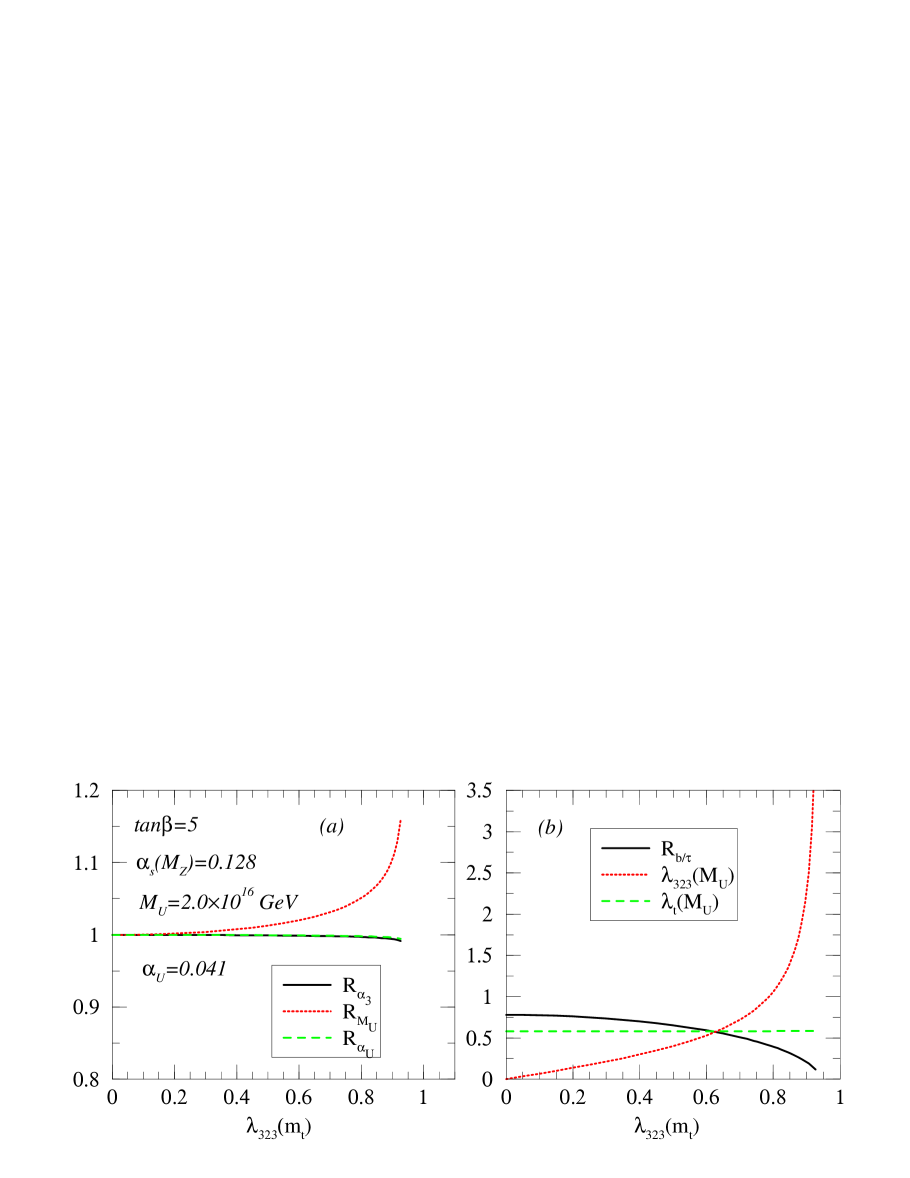
Figure 1: Effect of non-zero $\not\!\!R_{p}$ coupling $\lambda_{323}$ upon unification predictions. The value of $\tan\beta$ input and the predictions for no $\not\!\!R_{p}$ are shown in the figures. (a) $R_{i}$ correspond to the ratio of the prediction of $i$ in the $R_{p}$ case to the predictions in the $\not\!\!R_{p}$ case. (b) $R_{b/\tau}=\lambda_{b}(M_{U})/\lambda_{\tau}(M_{U})$.

4 Outline of the Numerical Analysis of RGEs

In order to determine the scale of unification we numerically solve the renormalisation group equations. In the process, we re-derive unification predictions in the MSSM [7, 17, 20], [41]-[44]. The main aim of this paper is to isolate the new effects due to the SUSY $\not\!\!R_{p}$ part of the theory. When running the equations we must cross the mass thresholds of the supersymmetric particles. In order to determine these we must also run the two-loop RGEs of the soft supersymmetry breaking terms. The $\not\!\!R_{p}$ couplings contribute to these RGEs, but this contribution has not yet been calculated at two-loop, although one-loop RGEs exist [32]. In the future, when the full RGEs for the soft terms have been calculated, it will be interesting to include the $\not\!\!R_{p}$ effects on the spectrum and thus on the thresholds. At this stage, we make the approximation of using the $R_{p}$-MSSM RGEs for the soft terms and the above $\not\!\!R_{p}$ RGEs for the dimensionless couplings. We will also not consider (potentially large, but model dependent) GUT threshold corrections [42, 44].

We add in turn one of the three $\not\!\!R_{p}$-Yukawa couplings (3.1). We run the full set of equations including the two-loop correction of the Yukawa couplings to the running of the gauge couplings in Eq. (2.8). The boundary values of the running $\overline{DR}$ gauge couplings $g_{1}(M_{Z})$ and $g_{2}(M_{Z})$ can be determined in terms of the experimentally well known parameters, the Fermi constant $G_{F}$, the Z-boson mass $M_{Z}$ and the electromagnetic coupling $\alpha_{EM}^{-1}$ at $Q^{2}=0$.

$$G_{F} = 1.16639\,10^{-5}\,GeV^{-2},$$ (4.1)

$$M_{Z} = 91.187\mbox{~{}GeV},$$ (4.2)

$$\alpha_{EM}^{-1}(Q^{2}=0) = 137.036.$$ (4.3)

For a given set of pole masses $m_{t}=174\mbox{~{}GeV}$, $m_{b}=4.9\mbox{~{}GeV}$, $m_{\tau}=1.777\mbox{~{}GeV}$ we define the $\overline{DR}$ Yukawa couplings at $M_{Z}$. Then we use 2-loop Renormalisation Group equations to run up to the scale $M_{U}$, where $g_{1}$ and $g_{2}$ meet.

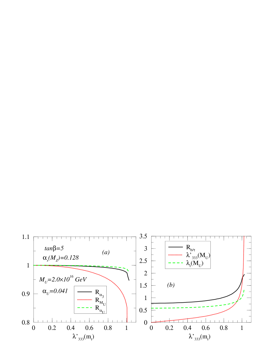
Figure 2: Effect of non-zero $\not\!\!R_{p}$ coupling $\lambda_{333}^{\prime}$ upon unification predictions. The value of $\tan\beta$ input and the predictions for no $\not\!\!R_{p}$ are shown in the figures. (a) $R_{i}$ correspond to the ratio of the prediction of $i$ in the $R_{p}$ case to the predictions in the $\not\!\!R_{p}$ case. (b) $R_{b/\tau}=\lambda_{b}(M_{U})/\lambda_{\tau}(M_{U})$.

We have assumed universal boundary conditions at $M_{U}$ for the soft breaking parameters $A_{0}$, $M_{0}$, $M_{1/2}$. The iteration procedure used to determine our results is described in [44]. As a characteristic mean value of the soft breaking parameters at $M_{U}$ we choose $A_{0}=M_{1/2}=M_{0}=300\mbox{~{}GeV}$. We solve the RGEs for different values of the $\not\!\!R_{p}$-coupling at $m_{t}$, starting from zero. The maximal value we consider is where the running coupling reaches the perturbative limit at the unification scale. For most of our discussion we take this to be $\lambda(M_{U})<\sqrt{4\pi}\approx 3.5$. However, we also show some results where $\lambda(M_{U})<5.0$.

There has been a large interest in the literature [7, 20, 17, 18, 19, 46] in the restrictions on the unification scenario from bottom-tau unification. Requiring bottom-tau unification leads to a strict relation between the running top quark mass and $\tan\beta$. For the experimental value of $m_{t}$ [21], $\tan\beta$ is predicted to be very close to 1.5 or around 55 [47]. We are interested in how the effects of $\not\!\!R_{p}$ can relax this strict relation and allow a larger range of $\tan\beta$. As a model scenario, we consider $\tan\beta=5$ which is well away from the solutions in the MSSM. We show that this feature is general and that solutions may be obtained for any value of $\tan\beta$, provided one tunes the value of the $\not\!\!R_{p}$ coupling. The $\not\!\!R_{p}$ couplings change the fixed-point (and quasi-fixed point) structure of the top-Yukawa coupling’s evolution. This is investigated in detail for low values of $\tan\beta$.

5 Gauge Coupling Unification

For $\lambda_{\not R_{p}}=0$ and with the inputs and procedure defined above, we obtain

$$\alpha_{s}(M_{Z})=0.128,\quad M_{U}=2.0\,10^{16}\mbox{~{}GeV},\quad\alpha_{U}=0.041.$$ (5.1)

In order to discuss the effects of the non-zero $\not\!\!R_{p}$ Yukawa couplings we consider the unification parameters as functions of $\lambda_{\not R_{p}}$ evaluated at $m_{t}$.

$$\alpha_{s}(M_{Z},\lambda_{\not R_{p}}),\quad M_{U}(\lambda_{\not R_{p}}),\quad\alpha_{U}(\lambda_{\not R_{p}}).$$ (5.2)

and define the ratios

$$R_{\alpha_{3}}(\lambda_{\not R_{p}}) = \frac{\alpha_{3}(M_{Z},\lambda_{\not R_{p}})}{\alpha_{3}(M_{Z},0)},$$

$$R_{M_{U}}(\lambda_{\not R_{p}}) = \frac{M_{U}(\lambda_{\not R_{p}})}{M_{U}(0)},$$ (5.3)

$$R_{\alpha_{U}}(\lambda_{\not R_{p}}) = \frac{\alpha_{U}(\lambda_{\not R_{p}})}{\alpha_{U}(0)}.$$

When $\lambda_{\not R_{p}}=0$ and $\tan\beta=5$, the ratios in (5.3) are then all equal to 1 as can be seen on the left of Figs. 1a, 2a, and 3a, respectively.

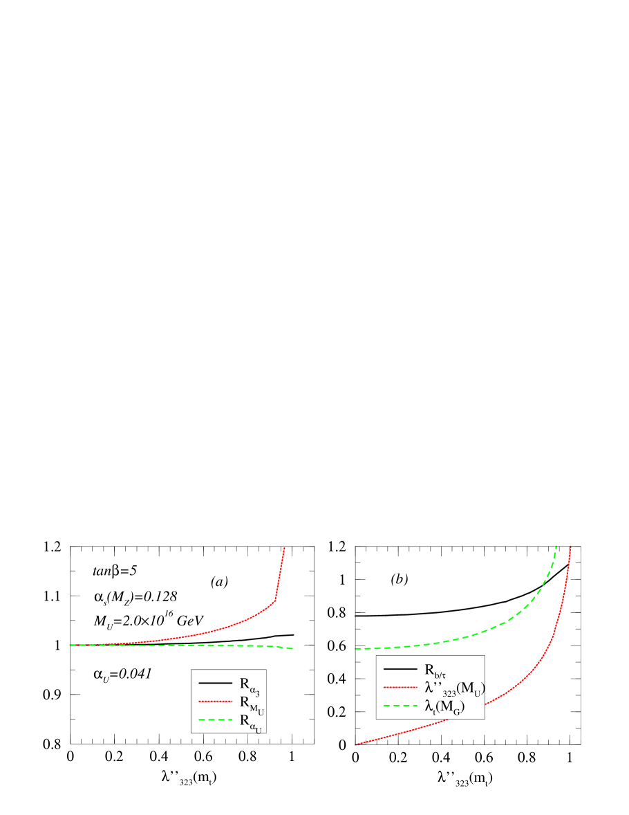
Figure 3: Effect of non-zero $\not\!\!R_{p}$ coupling $\lambda_{323}^{\prime\prime}$ upon unification predictions. The value of $\tan\beta$ input and the predictions for the no $\not\!\!R_{p}$ case are shown in the figures. (a) $R_{i}$ correspond to the ratio of the prediction of $i$ in the $R_{p}$ case to the predictions in the $\not\!\!R_{p}$ case. (b) $R_{b/\tau}=\lambda_{b}(M_{U})/\lambda_{\tau}(M_{U})$.

Next we turn on the $\not\!\!R_{p}$-couplings. In Fig.s 1b, 2b, and 3b we can read off the value of the $\not\!\!R_{p}$-coupling at the unification scale as a function of the coupling at $m_{t}$. The plots stop once the perturbative limits are reached. For the present numerical discussion we focus on $\tan\beta=5$. $\lambda_{323}(M_{U})$ reaches its perturbative limit for a low scale value of $\lambda_{323}(m_{t})=0.93$. It is worth pointing out that this is the same as the laboratory bound for slepton masses at $1.5\mbox{~{}TeV}$! Thus although the laboratory bounds on the $LL{\bar{E}}$ operators are generally considered to be very strict; for heavy supersymmetric masses they are no stricter than the perturbative limit. At this point $\lambda_{323}$ has run off Fig. 1b but it should be clear how it extrapolates. The perturbative limits for the other couplings are given by

$${\lambda^{\prime}}_{333}(m_{t}) = 1.06$$ (5.4)

$${\lambda^{\prime\prime}}_{323}(m_{t}) = 1.07$$ (5.5)

The first limit (5.4) is equivalent to the empirical 2 $\sigma$ limit for $700\mbox{~{}GeV}$ squark masses. The 1$\sigma$ empirical bound on ${\lambda^{\prime\prime}}_{323}$ is 0.43 for $100\mbox{~{}GeV}$ squark mass, and so the limit (5.5) will be restrictive for somewhat higher masses. These limits are $\tan\beta$ dependent, and we leave a full discussion to section 7.3.1.

In Fig.s 1a, 2a, 3a we show how the ratios (5.3) change as we turn on the $\not\!\!R_{p}$-couplings. For $\lambda_{323}\not=0$, $\alpha_{s}(M_{Z})$ and $\alpha_{U}$ are practically unchanged except very close to the perturbative limit. However, $M_{U}$ is shifted upwards by up to $10(15)\%$, where the parenthesised value corresponds to choosing the perturbative limit to be $\lambda<5.0$. For ${\lambda^{\prime}}_{333}$ the downward shift in $\alpha_{s}(M_{Z})$ is typically 1-2%. At the extreme perturbative limit $\lambda<5.0$ the maximum shift is is a decrease of $5\%$ in $\alpha_{s}(M_{Z})$ giving a value of $\alpha_{s}(M_{Z})=0.122$. This corresponds to an agreement with the data $\alpha_{S}(M_{Z})=0.119\pm 0.002$ [48] to 1.5$\sigma$, without using GUT threshold corrections. While the importance of this result is obvious, caution in its interpretation is required because the correction to $\alpha_{S}(M_{Z})$ is sensitive to where one places the limit of perturbative believability. For example, if one chooses $\lambda(M_{U})<3.5$, one only obtains a 3$\%$ decrease, still with significantly better agreement with the data than the $R_{p}$ conserving case. $\alpha_{U}$ is decreased slightly at this point. However, $M_{U}$ is decreased by up to $20\%$. This effect is significantly beyond the effect due to the top quark Yukawa coupling. For ${\lambda^{\prime\prime}}_{323}\not=0$, $\alpha_{U}$ remains practically unchanged. $\alpha_{s}$ now has an overall increase of up to about $3\%$ at the perturbative limit corresponding to a value of $\alpha_{s}(M_{Z})=0.131$ in disagreement with the experimental value. $M_{U}$ is raised by up to $20\%$.

Thus we find $\alpha_{U}$ essentially unchanged by $\not\!\!R_{p}$-effects. $M_{U}$ can change either way by up to $20\%$. If we compare this with other effects considered in Ref. [41] we find it of the same order as the uncertainty due to the top quark Yukawa coupling or the effects of possible non-renormalisable operators at beyond the GUT scale. The effect is much smaller than that due to GUT-scale threshold corrections or weak-scale supersymmetric threshold corrections. It is thus much too small an effect to accommodate string unification. The strong coupling can also change either way by up to $5\%$. A decrease is favoured by the data and is welcome in supersymmetric unification. The effect of the $\not\!\!R_{p}$-couplings on $\alpha_{s}(M_{Z})$ is of the same order as the effects due to the top-quark Yukawa coupling, GUT-scale threshold effects and high-scale non-renormalisable operators [41].

6 b-$\tau$ Unification

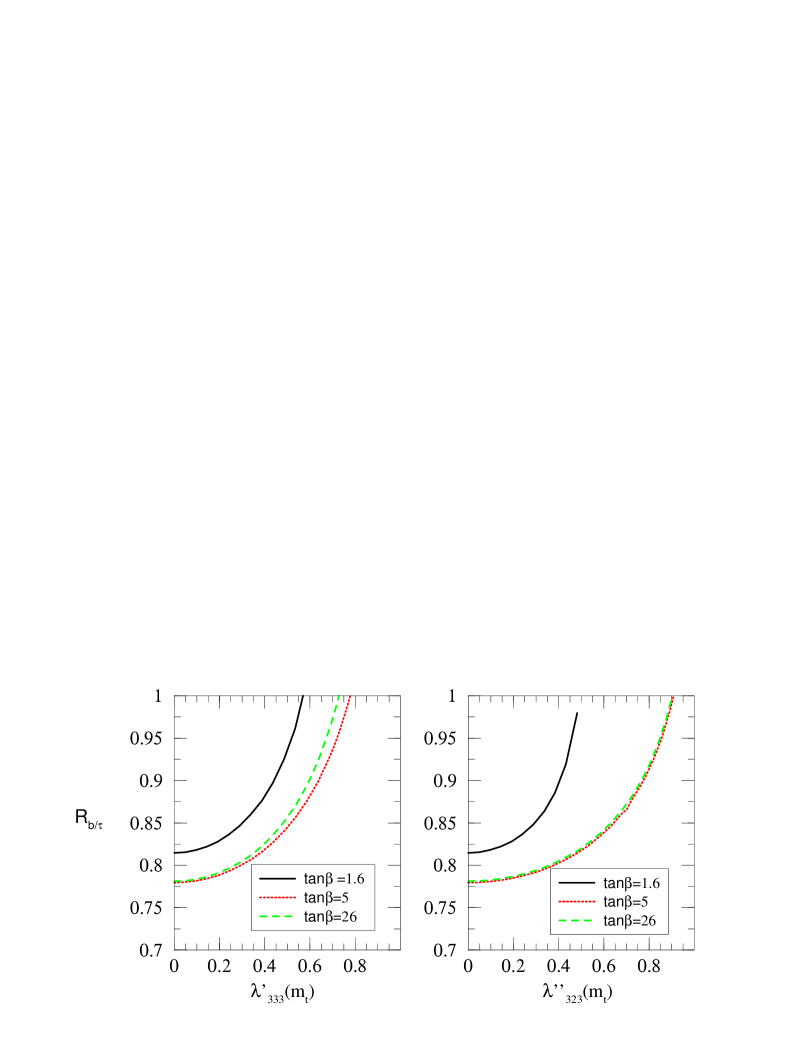
Figure 4: Bottom-tau Yukawa unification including the R-parity violating couplings (a) $\lambda_{333}^{\prime}$, (b) $\lambda^{\prime\prime}_{323}$ for various $\tan\beta=1.6,5,26$. The plots show $R_{b/\tau}=\lambda_{b}(M_{U})/\lambda_{\tau}(M_{U})$ as a function of the $\not\!\!R_{p}$ couplings evaluated at $m_{t}$. In (b), the $\tan\beta=1.6$ curve stops as $\lambda_{t}(M_{U})$ reaches its perturbative limit.

In order to study the unification of the bottom and $\tau$ Yukawa couplings $\lambda_{b},\,\lambda_{\tau}$ at $M_{U}$ we define the ratio

$$R_{b/\tau}(M_{U})=\frac{\lambda_{b}(M_{U},\lambda_{\not R_{p}})}{\lambda_{\tau}(M_{U},\lambda_{\not R_{p}})}.$$ (6.1)

For $\lambda_{\not R_{p}}=0$, $\tan\beta=5$ we have

$$R_{b/\tau}(M_{U})=0.78.$$ (6.2)

Thus including the top-quark effects but before turning on the $\not\!\!R_{p}$-coupling we are well away from the bottom-tau unification solution $R_{b/\tau}(M_{U})=1$. Recall that the uncertainties due to the bottom quark mass are small for small $\tan\beta$. Now we consider the corrections due to the $\not\!\!R_{p}$-couplings. The one-loop RGE for $R_{b/\tau}(t)$ is given by

$$16\pi^{2}\frac{dR_{b/\tau}(t)}{dt}=R_{b/\tau}(t)\left[\lambda_{t}^{2}+3\lambda_{b}^{2}-3\lambda_{\tau}^{2}-4\lambda_{323}^{2}+3{\lambda^{\prime}}_{323}^{2}+2\lambda^{{}^{\prime\prime}2}_{323}+\frac{4}{3}g_{1}^{2}-\frac{16}{3}g_{3}^{2}\right].$$ (6.3)

The leading dependence of $R_{b/\tau}$ on $\lambda_{323}$ has a negative sign and as we see in the two-loop result shown in Fig. 1b $R_{b/\tau}$ drops significantly. Near the perturbative limit it drops by a factor of 2.5 and $\not\!\!R_{p}$  becomes a dominant effect on the evolution of $R_{b/\tau}$. This is important for the range of $\tan\beta$ which leads to bottom-tau unification. In the MSSM $R_{b/\tau}$ is too large for $\tan\beta\stackrel{{\scriptstyle<}}{{\sim}}1.5$ or $\,\,\stackrel{{\scriptstyle>}}{{\sim}}55$ [47]. Including a non-zero operator $\lambda_{323}$ strongly reduces $R_{b/\tau}$ and thus can lead to bottom-tau unification in this previous regime.

For ${\lambda^{\prime\prime}}_{323}\not=0$ or ${\lambda^{\prime}}_{333}\not=0$ there is an additional positive contribution in the evolution of $R_{b/\tau}(t)$. The full two-loop result shows a clear rise in $R_{b/\tau}(t)$ as a function of ${\lambda^{\prime\prime}}_{323}$ in Fig. 3b. The maximum increase at the perturbative limit is by $60\%$. For ${\lambda^{\prime\prime}}_{323}(m_{t})=0.9$ bottom-tau unification is restored! This is quite remarkable. Even though $\not\!\!R_{p}$-couplings are usually expected to lead to only small effects they can have a significant impact on our understanding of Yukawa-unification. Recall, that grand unification is possible in $\not\!\!R_{p}$-theories as discussed extensively in the introduction. From Eq. (6.3) it should be clear that for example for ${\lambda^{\prime}}_{333}$ we get an increase in $R_{b/\tau}(M_{U})$ as well leading to further bottom-tau unification points. From Fig. 2, we see that for ${\lambda^{\prime}}_{333}(m_{t})=0.75$, we achieve $R_{b/\tau}=1$ for $\tan\beta=5$. To investigate further, we plot $R_{b/\tau}$ as a function of ${\lambda^{\prime}}_{333}(m_{t})$ for several other values of $\tan\beta$ in Fig. 4a. The figure illustrates that any value of $\tan\beta=2-26$ achieves bottom-tau Yukawa unification, provided ${\lambda^{\prime}}_{333}(m_{t})$ is chosen correctly. Fig. 4b shows the equivalent plot for ${\lambda^{\prime\prime}}_{323}\not=0$ with the same conclusions.

7 Landau Poles and Fixed Points of Yukawa Couplings

True fixed points and quasi fixed points were first considered in [49]. Since then, many applications have been discussed in the literature (see ref.[50] and references therein), including those in the $R_{p}$ conserving MSSM. In the MSSM and at low $\tan\beta$, it is well known that if one neglects two-loop corrections as well as those from couplings smaller than $g_{3}$, the RGE for $\lambda_{t}$ has an infra-red stable fixed point [25] corresponding to $\lambda_{t}/g_{3}=\sqrt{7/18}$. This is too low to accommodate $m_{t}=175\pm 5\mbox{~{}GeV}$. To be phenomenologically viable, $\lambda_{t}$ must be out of the domain of attraction of the true fixed-point. In practice, this implies that $\lambda_{t}(m_{t})$ must be nearer to its quasi-fixed point (QFP) limit of 1.1, where $\lambda_{t}(M_{U})$ is large (formally it diverges). Using $m_{t}(m_{t})=165\pm 5\mbox{~{}GeV}$ as an input means that one can derive $\tan\beta$ in this scenario through the relation

$$\sin\beta=\frac{\sqrt{2}m_{t}(m_{t})}{v\lambda_{t}(m_{t})},$$ (7.1)

implying $\tan\beta=1.7\pm 0.2$ at the QFP [51]. This scenario is very attractive [26, 50] because the values of many parameters in the infra-red regime are insensitive to their input values at $M_{U}$, giving higher predictivity and a tightly constrained phenomenology. The quasi-fixed $R_{p}$ conserving MSSM is presently severely constrained [51, 50]. A large $\not\!\!R_{p}$ coupling changes the running significantly, and so in this section, we examine the running of the couplings as a function of renormalisation scale. It is convenient to split this analysis into three cases to focus upon: (1) infra-red stable fixed points of approximated RGEs, (2) a small amount of $\not\!\!R_{p}$ near the QFP of $\lambda_{t}$ and (3) the case of two large Yukawa couplings. We then examine the constraints on the $\not\!\!R_{p}$ couplings defined at $m_{t}$ coming from the requirement of perturbativity up to $M_{U}$.

7.1 Fixed Points

First, we analyse the fixed points in the equations including the couplings $\lambda^{\prime}_{333},\lambda^{\prime\prime}_{323}$ one at a time. Neglecting $\lambda_{b},\lambda_{\tau}$ (i.e. looking at the low $\tan\beta$ limit) and two-loop terms, we reformulate Eqs. (3.19), (3.14)-(3.16) as

$$\frac{d\ln X_{t}}{d\ln g_{3}^{2}} = \frac{7}{9}-\frac{1}{3}X^{\prime}-2X_{t}-\frac{2}{3}X^{\prime\prime}+\frac{\alpha_{2}}{\alpha_{3}}+\frac{13}{45}\frac{\alpha_{1}}{\alpha_{3}}$$ (7.2)

$$\frac{d\ln X}{d\ln g_{3}^{2}} = -1+\frac{3}{5}\frac{\alpha_{1}}{\alpha_{3}}+\frac{\alpha_{2}}{\alpha_{3}}-\frac{4}{3}X$$ (7.3)

$$\frac{d\ln X^{\prime}}{d\ln g_{3}^{2}} = \frac{7}{9}-\frac{1}{3}X_{t}-2X^{\prime}+\frac{\alpha_{2}}{\alpha_{3}}+\frac{7}{45}\frac{\alpha_{1}}{\alpha_{3}}$$ (7.4)

$$\frac{d\ln X^{\prime\prime}}{d\ln g_{3}^{2}} = \frac{5}{3}-2X^{\prime\prime}-\frac{2}{3}X_{t}+\frac{4}{5}\frac{\alpha_{1}}{\alpha_{3}},$$ (7.5)

where $X_{t}\equiv\lambda_{t}^{2}/g_{3}^{2}$, $X\equiv{\lambda}_{323}^{2}/g_{3}^{2}$, $X^{\prime}\equiv{\lambda^{\prime}}_{333}^{2}/g_{3}^{2}$ and $X^{\prime\prime}\equiv{\lambda^{\prime\prime}}_{323}^{2}/g_{3}^{2}$. The stability of Yukawa couplings in supersymmetric theories has been considered in refs. [52]. Considering only one non-zero $\not\!\!R_{p}$ coupling at a time, we have two infra-red stable fixed points in the limit that we ignore the electroweak gauge couplings. The first is

$$X=X^{\prime}=0:\qquad X_{t}=\frac{1}{8},\qquad X^{\prime\prime}=\frac{19}{24}$$ (7.6)

and the second is

$$X=X^{\prime\prime}=0:\qquad X_{t}=X^{\prime}=\frac{1}{3}.$$ (7.7)

We have ignored $\lambda_{323}$ in this discussion because it does not exhibit fixed point behaviour itself due to the lack of renormalisation from the QCD interactions. The values of $X_{t}$ in Eqs. (7.6),(7.7) are even lower than the $R_{p}$-conserving MSSM value $X_{t}=7/18$. They are experimentally excluded [50] by the lower bound on $\lambda_{t}(m_{t})$ coming from the requirement of $m_{t}(m_{t})=165\mbox{~{}GeV}$.

7.2 Large $\lambda_{t}(M_{U})$, Small $\not\!\!R_{p}$ Coupling

We now discuss the case where $\lambda_{t}(M_{U})>1$ and the $\not\!\!R_{p}$-couplings are in turn very small. The behaviour of the $R_{p}$ conserving superpotential parameters will be similar to their behaviour in the $R_{p}$ conserving MSSM. In this case, we can solve the one-loop RGEs for the $\not\!\!R_{p}$ Yukawa couplings analytically:

$${\lambda}_{323}(\mu) = {\lambda}_{323}(M_{U})\delta_{2}^{-3}\delta_{1}^{-3/11},$$ (7.8)

$${\lambda^{\prime}}_{333}(\mu) = {\lambda^{\prime}}_{333}(M_{U})\delta_{3}^{40/27}\delta_{2}^{-5/2}\delta_{1}^{-29/594}\delta_{t}^{1/6},$$ (7.9)

$${\lambda^{\prime\prime}}_{323}(\mu) = {\lambda^{\prime\prime}}_{323}(M_{U})\delta_{3}^{56/27}\delta_{2}\delta_{1}^{-95/297}\delta_{t}^{1/3},$$ (7.10)

where $\delta_{1,2,3}\equiv g_{1,2,3}(\mu)/g(M_{U})$ and $\delta_{t}\equiv\lambda_{t}(\mu)/\lambda_{t}(M_{U})$. We have neglected contributions from $\lambda_{\tau},\lambda_{b}$ in Eqs. (7.8)-(7.10) and so they are valid only at low $\tan\beta<15$. The one-loop analytic solutions for $\delta_{1,2,3}$ are equivalent to the $R_{p}$ conserving MSSM ones [50]. The solution for $\delta_{t}$ is also equivalent to its $R_{p}$ counterpart, which has been solved analytically at one loop order including $g_{3},g_{2}$ [53]. Eqs. (7.8)-(7.10) predict a constant ratio of $\lambda_{\not R_{p}}(M_{U})/\lambda_{\not R_{p}}(m_{t})$. This corresponds to a straight line for the $\lambda_{\not R_{p}}(M_{U})$ curves in Figs. 1b, 2b, 3b. For $\lambda_{\not R_{p}}(m_{t})\stackrel{{\scriptstyle<}}{{\sim}}0.3$ this is a good approximation, after that the two-loop effects become important. We also obtain analytic solutions at low $\tan\beta$ for the bi-linear $\not\!\!R_{p}$ terms when the $\not\!\!R_{p}$ Yukawa couplings are small:

$$\kappa_{i}(\mu)=\kappa_{i}(M_{U})\delta_{1}^{-5/198}\delta_{2}^{-3/2}\delta_{3}^{-8/9}\delta_{t}^{1/2}.$$ (7.11)

7.3 Two large Yukawa couplings

The one-loop RGEs including $\lambda_{t}$, $\lambda_{b}$, $g_{2,3}$ have been solved in the MSSM [54]. These RGEs have the same form in the case of a non-zero $\lambda^{\prime}_{333}$, when ignoring all other Yukawa couplings except $\lambda_{t}$. The analytic solutions to this system are therefore contained in ref. [54] and are in terms of hypergeometric functions.

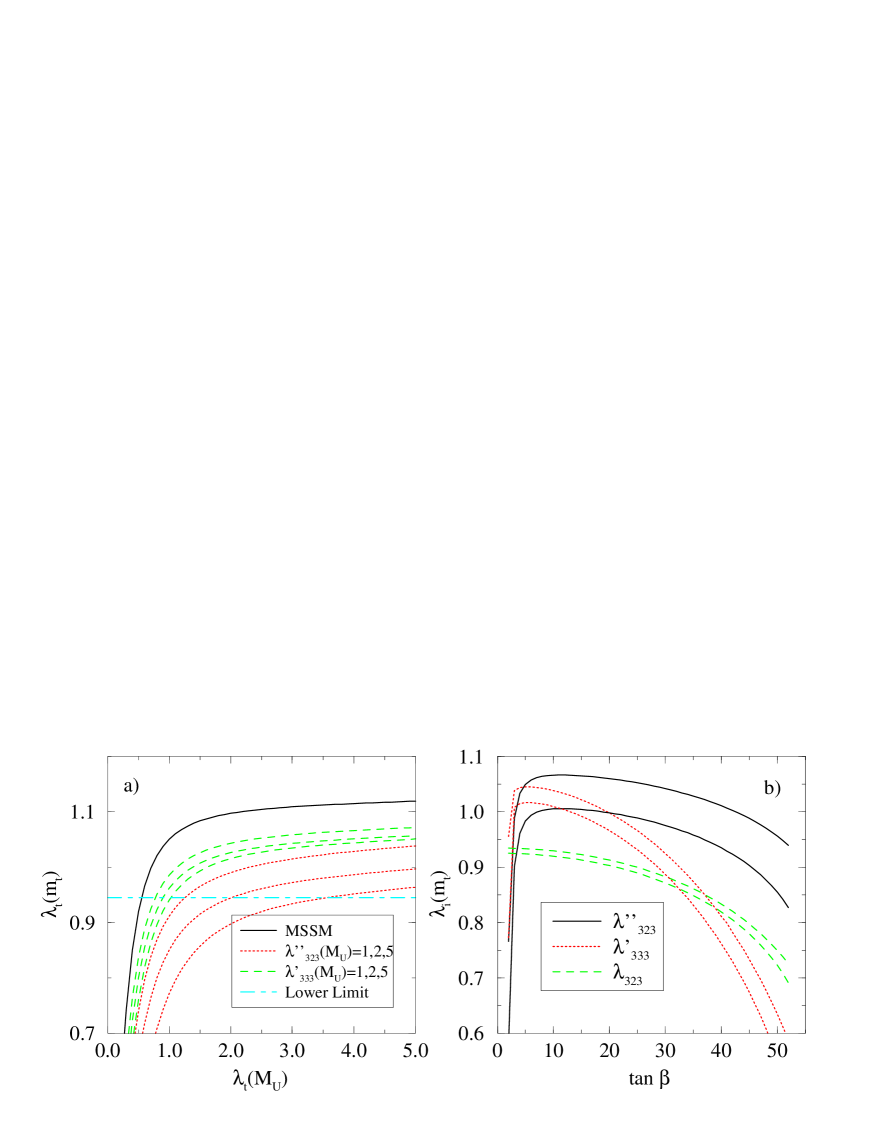
Figure 5: (a) Effect of large R-parity violating couplings upon the quasi-fixed point of $\lambda_{t}$. The $\not\!\!R_{p}$ couplings increase toward the bottom of the plot. The lower limit of $\lambda_{t}(m_{t})$ is defined as the minimum value required to obtain $m_{t}(m_{t})=165\mbox{~{}GeV}$. (b) Perturbative limits of large R-parity violating couplings as a function of $\tan\beta$. The upper curves correspond to the two-loop order calculation and the lower ones to a one-loop calculation.

We present here numerical solutions to the two-loop equations, which can also be applied to the cases of large ${\lambda}_{323}$, or ${\lambda^{\prime\prime}}_{323}$ with large $\lambda_{t}(m_{t})$. Using $\alpha_{U}=0.041$, $M_{U}=2\times 10^{16}\mbox{~{}GeV}$ and again switching off $\lambda_{b}$ and $\lambda_{\tau}$ (which is only valid for low $\tan\beta\stackrel{{\scriptstyle<}}{{\sim}}15$), we calculate how $\lambda_{t}(m_{t})$ is related to its input value at $M_{U}$, i.e. we study the quasi-fixed point structure. SUSY threshold corrections are not included.

In Fig. 5a, the top solid line shows the quasi-fixed point structure of $\lambda_{t}$ in the MSSM. For $\lambda_{t}(M_{U})>2.0$ it is almost flat, i.e. $\lambda_{t}(m_{t})=1.1$ becomes insensitive to $\lambda_{t}(M_{U})$. The horizontal dashed line corresponds to the minimum $\lambda_{t}(m_{t})$ required to produce a top quark mass which agrees with the data and for which $\sin\beta\leq 1$. It changes by $\pm 0.03$ within the empirical errors on $m_{t}$. The $\lambda_{323}\not=0$ curves are not plotted because they coincide with that of the MSSM. This can be understood from Eq. (3.19) as the coupling does not directly appear in the running of $\lambda_{t}$. This holds at two-loop due to our assumption of only one dominant $\not\!\!R_{p}$ coupling at a time.

When ${\lambda^{\prime}}_{333}$ is switched on, the quasi-fixed point behaviour of $\lambda_{t}$ persists but its QFP value can be decreased as far as $\lambda_{t}(m_{t})=1.03$ which corresponds to $\tan\beta=2.1\pm^{0.9}_{0.1}$. Any decrease in $\lambda_{t}(m_{t})$ can increase $\tan\beta$ as extracted from Eq. (7.1), modifying the QFP predictions of superpartner masses, for example. In particular, higher $\tan\beta$ can allow for higher masses of the lightest CP-even Higgs, relaxing a severe constraint in the $R_{p}$ conserving QFP scenario [51]. For large ${\lambda^{\prime\prime}}_{323}$, the quasi-fixed behaviour of $\lambda_{t}$ is somewhat weakened as the non-zero gradient of the curves suggests, but $\lambda_{t}(m_{t})=1$ is possible as the QFP prediction, corresponding to $\tan\beta=3.0\pm^{1.5}_{0.7}$.

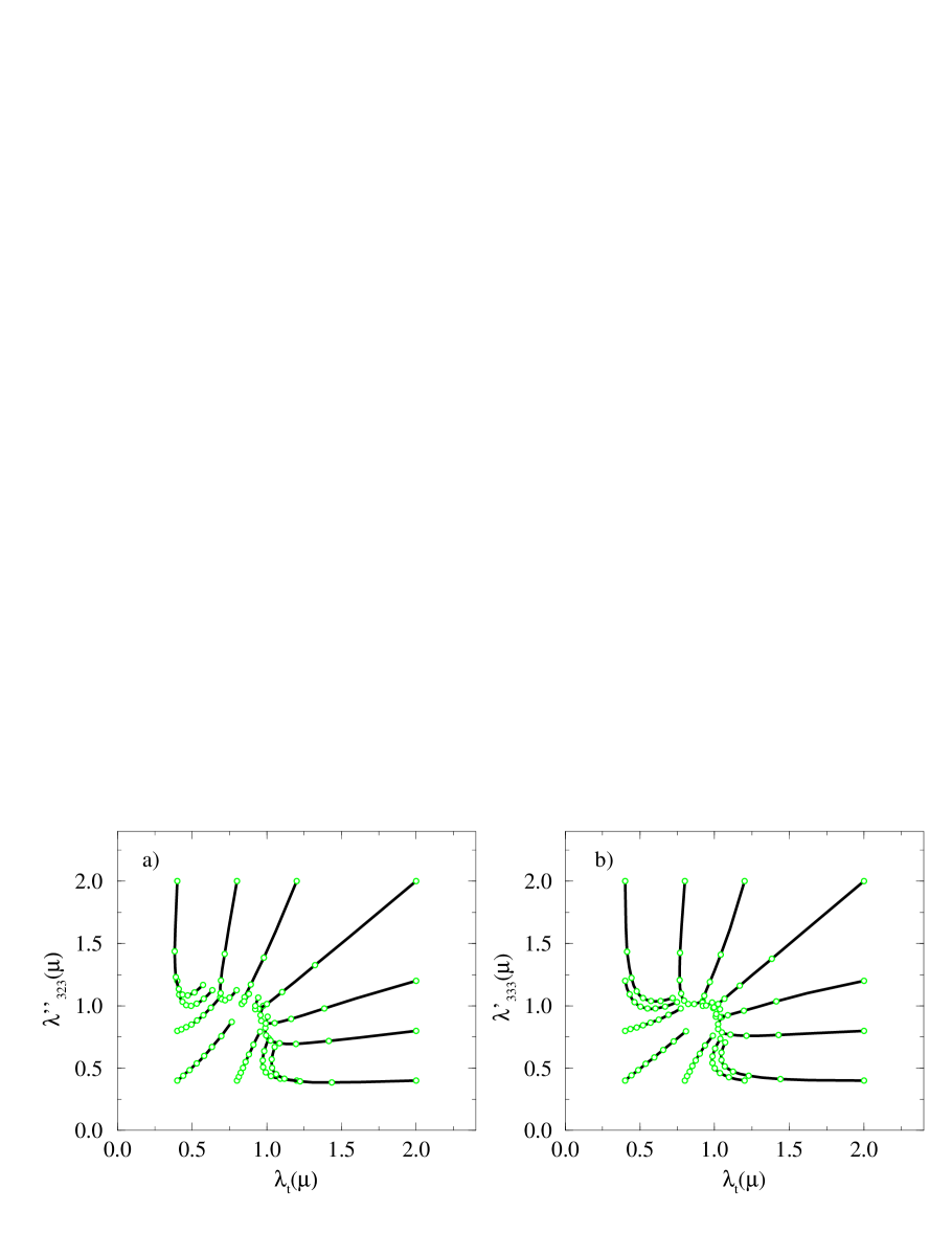
Figure 6: Running of $\lambda_{t}(\mu)$ and (a) $\lambda^{\prime\prime}_{323}(\mu)$, (b) $\lambda^{\prime}_{333}(\mu)$. The circles are separated by two orders of magnitude of $\mu$/ GeV. The flow is towards the region (a) $\lambda_{t}\approx 1,{\lambda^{\prime\prime}}_{323}\approx 1$ and (b) $\lambda_{t}\approx 1,{\lambda^{\prime}}_{333}\approx 1$ for decreasing $\mu$.

Fig. 5 only shows information on the quasi-fixed point structure of $\lambda_{t}$. One would like to know if the $\not\!\!R_{p}$ couplings also exhibit the QFP behaviour when they are large. Fig. 6a shows the running of both $\lambda_{t}(\mu)$ and $\lambda^{\prime\prime}_{323}(\mu)$ with the renormalisation scale $\mu$. $\lambda_{b}$, $\lambda_{\tau}$ have been switched off in this calculation. The two-loop $\not\!\!R_{p}$-MSSM RGEs were run through 14 orders of magnitude (roughly corresponding to running from $M_{U}$ to $m_{t}$), using $\alpha_{U}=0.041$. Although the figure shows both couplings running toward 1 in the infra-red regime, it is clear that it is difficult to make this statement quantitatively accurate. The same conclusion holds for large $\lambda^{\prime}_{333}\not=0$ and $\lambda_{t}$, as shown in Fig. 6b. $\lambda_{323}$ exhibits even less focussing behaviour because it is not directly affected by QCD interactions.

7.3.1 Perturbative Limits

In Fig. 5b, we show the limits from perturbativity upon the $\not\!\!R_{p}$-couplings defined at $m_{t}$. We use a degenerate effective SUSY spectrum at $m_{t}$ in this calculation but no finite SUSY threshold effects are included. We include $\lambda_{\tau}$, $\lambda_{b}$ however, because they make a large difference to any Landau poles of Yukawa couplings at high $\tan\beta$. When we switch an $\not\!\!R_{p}$ coupling on, the curves in the figure map out what value of the coupling is required at $m_{t}$ to produce a value of 5 for at least one of the Yukawa couplings at $M_{U}$. In practice, to good accuracy the point where a Yukawa coupling is 5 is very close to the Landau pole of that coupling. The deviation between the two curves shows the significant weakening effect of including two-loop terms in the RGEs: 5$\%$, 12$\%$ and 10$\%$ for $\lambda_{323}$, $\lambda^{\prime}_{323}$ and $\lambda^{\prime\prime}_{323}$ at high $\tan\beta$ respectively. The upper bound calculated in this way exhibits a strong $\tan\beta$ dependence due to $\lambda_{b}$, $\lambda_{\tau}$ contributing to the running at high $\tan\beta$. Our one-loop bounds in Fig 5b agree with the previous limits upon $\lambda^{\prime\prime}_{323}$ from perturbativity bounds provided in by Brahmachari and Roy [36] to within 3%. One-loop bounds upon other $\lambda^{\prime\prime}_{ijk}$ were obtained by Goity and Sher [36].

8 Conclusions

We have argued that $\not\!\!R_{p}$ is theoretically on equal footing with conserved $R_{p}$. Since it can be realized in grand unified theories it is relevant for unification. We then first determined the complete two-loop renormalisation group equations for the dimensionless couplings of the unbroken supersymmetric Standard Model. It is only at two-loop that Yukawa couplings affect the running of the gauge coupling constants. We then considered three models of $\not\!\!R_{p}$. We have added to the MSSM in turn the three Yukawa operators $L_{3}L_{2}{\bar{E}}_{3}$, $L_{3}Q_{3}{\bar{D}}_{3}$, and ${\bar{U}}_{3}{\bar{D}}_{2}{\bar{D}}_{3}$. We considered their effects on various aspects of the perturbative unification scenario. We have focused on qualitative effects. A detailed search for a preferred model is beyond the scope of this paper. We found several important effects. The unification scale is shifted by up to $\pm 20\%$. This is comparable to some threshold effects but insufficient for string unification. $\alpha_{s}(M_{Z})$ can be changed at most by $\pm 5\%$. The reduction which is favoured by the data is obtained close to the perturbative limits of ${\lambda^{\prime}}_{333}$ and $\lambda^{\prime\prime}_{323}$. We have obtained the two-loop limit from perturbative unification for all three operators. For $\lambda_{323}$ it is equivalent to the laboratory bound for a slepton mass of $1.5\mbox{~{}TeV}$ and for $\lambda^{\prime}_{333},\lambda^{\prime\prime}_{323}$ is competitive for masses below $1\mbox{~{}TeV}$. Two-loop limits from perturbativity are $5-12\%$ weaker than the one-loop limit previously obtained. This is all quite remarkable. The $\not\!\!R_{p}$-couplings can have significant effects on the entire Yukawa unification picture. For bottom-tau unification we have found significant affects. For $\lambda_{323}\not=0$ bottom-tau unification could be obtained for values of $\tan\beta<1.5$ were it not for the fact that the perturbative limit is reached. For $\lambda^{\prime\prime}_{323},\lambda^{\prime}_{333}\not=0$, we found new points of bottom-tau unification at $\tan\beta=5-26$. Thus for $\tan\beta<30$, bottom-tau unification doesn’t necessarily correspond to top IR quasi fixed-point structure, as is the case in the MSSM [7, 25, 27, 50]. Indeed, the quasi-fixed structure is changed resulting in lower values of the $\lambda_{t}(m_{t})$ prediction for $\lambda^{\prime}_{333},\lambda^{\prime\prime}_{323}$. This allows $\tan\beta$ to increase, resulting in higher masses for the lightest CP-even Higgs, relaxing severe constraints on the QFP.

Appendix

We consider a group $G$ with representation matrices ${\bf t}^{A}\equiv({\bf t})^{Aj}_{i}$. Then the quadratic Casimir $C(R)$ of a representation $R$ is defined by

$$({\bf t}^{A}{\bf t}^{A})^{j}_{i}=C(R)\delta^{j}_{i}.$$ (A.1)

For $SU(3)$ triplets $q$ and for $SU(2)_{L}$ doublets $L$ we have

$$C_{SU(3)}(q)=\frac{4}{3},\quad C_{SU(2)}(L)=\frac{3}{4}.$$ (A.2)

For $U(1)_{Y}$ we have

$$C(f)=\frac{3}{5}Y^{2}(f),$$ (A.3)

where $Y(f)$ is the hypercharge of the field $f$. The factor $3/5$ is the grand unified normalisation.

For the adjoint representation of the group of dimension $d(G)$ we have

$$C(G)\delta^{AB}=f^{ACD}f^{BCD},$$ (A.4)

where $f^{ABC}$ are the structure constants. Specifically for the groups we investigate

$$C(SU(3)_{C})=3,\quad C(SU(2)_{L})=2,\quad C(U(1)_{Y})=0,$$ (A.5)

and $C(SU(N))=N$. The Dynkin index is defined by

$$\mbox{Tr}_{R}({\bf t}^{A}{\bf t}^{B})\equiv S(R)\delta^{AB}.$$ (A.6)

For the respective fundamental representations $f$ we obtain

$$SU(3),\,SU(2):\quad S(f)=\frac{1}{2},$$ (A.7)

$$U(1)_{Y}:\quad S(f)=\frac{3}{5}Y^{2}(f),$$ (A.8)

where we have inserted the GUT normalisation for $U(1)_{Y}$.

The coefficients in the two-loop running of the gauge couplings (2.8) are given by [38]

$$B_{a}^{(1)} = (\frac{33}{5},1,-3),$$ (A.9)

$$B_{ab}^{(2)} = \left(\begin{array}[]{ccc}199/25&27/5&88/5\\ 9/5&25&24\\ 11/5&9&14\end{array}\right),$$ (A.13)

$$C_{a}^{u,d,e} = \left(\begin{array}[]{ccc}26/5&14/5&18/5\\ 6&6&2\\ 4&4&0\end{array}\right).$$ (A.17)

References

- [1] H. Georgi and S. Glashow, Phys. Rev. Lett. 32 (1974) 438.
- [2] H. Georgi, H.R. Quinn, S. Weinberg, Phys. Rev. Lett. (1974) 33.
- [3] W. Marciano, in Proceedings of the Workshop on Grand Unification, 16-18 April, 1987, Syracuse University, Syracuse, NY, edited by K.C. Wali (World Scientific, Singapore, 1988), pp 185-189.
- [4] U. Amaldi, et al., Phys. Rev. D36 (1987) 1385.
- [5] J. Ellis, S. Kelley and D.V. Nanopoulos, Phys. Lett. B 249 (1990) 131.
- [6] U. Amaldi, W. de Boer and H. Fürstenau, Phys. Lett. B 260 (1991) 447.
- [7] V. Barger, M.S. Berger and P. Ohmann, Phys. Rev. D 47 (1993) 1093.
- [8] P. Langacker, M.X. Luo, Phys. Rev. D 44 (1991) 817; R. G. Roberts and G. G. Ross, Nucl. Phys. B 377 (1992) 571.
- [9] For a review see for example H.P. Nilles, Phys. Rept. 110 (1984) 1.
- [10] H. Dreiner, published in ‘Perspectives on Supersymmetry’, Ed. by G.L. Kane, World Scientific, Singapore, 1998, hep-ph/9707435.
- [11] L. J. Hall and M. Suzuki, Nucl. Phys. B 231 (1984) 419.
- [12] L. Ibanez and G. G. Ross, Phys. Lett. B 260 (1991) 291; Nucl. Phys. B 368 (1992) 3.
- [13] G.F. Giudice, R. Rattazzi, Phys. Lett. B 406 (1997) 321, hep-ph/9704339.
- [14] K. Tamvakis, Phys. Lett. B 382 (1996) 251, hep-ph/9604343.
- [15] F. Vissani, Nucl. Phys. Proc. Suppl. 52A (1997) 94.
- [16] D. E. Brahm and L. J. Hall, Phys. Rev. D 40 (1989) 2449.
- [17] M. Chanowitz, J. Ellis and M. Gaillard, Nucl. Phys. B 128 (1977) 506; A. Buras, J. Ellis, M. Gaillard and D.V. Nanopoulos, ibid. B 293 (1978) 66; M.B. Einhorn and D.R.T. Jones, ibid. B 196 (1982) 475; J. Ellis, D.V. nanopoulos and S. Rudaz, ibid. B 202 (1982) 43; J. Ellis, S. Kelley, and D.V. Nanopoulos, Nucl. Phys. B 373 (1992) 55; M. Carena, M. Olechowski, S. Pokorski, and C.E.M. Wagner, Nucl. Phys. B 426 (1994) 269.
- [18] H. Arason, D.J. Castano, B. Keszthelyi, S. Mikaelian, E.J. Piard, P. Ramond and B. D. Wright, Phys. Rev. Lett. 67 (1991) 2933.
- [19] A. Dedes, K. Tamvakis, Phys. Rev. D 56 (1997) 1496.
- [20] M. Carena, S. Pokorski, and C.E.M. Wagner, Nucl. Phys. B 406 (1993) 59.
- [21] CDF Collaboration, F. Abe et al., Phys. Rev. Lett. 74 (1995) 2626; D0 Collaboration, S. Abachi et al., Phys. Rev. Lett. 74 (1995) 2632.
- [22] M.A. Diaz, J.C. Romao and J.W.F. Valle, Nucl. Phys. B 524 (1998) 23; A. Akeroyd, M.A. Diaz, J. Ferrandis, M.A. Garcia-Jareno and J.W.F. Valle, hep-ph/9707395; M.A. Diaz, J. Ferrandis, J.C. Ramao and J.W.F. Valle, hep-ph/9801391;
- [23] Savas Dimopoulos, Lawrence J. Hall, Stuart Raby Phys. Rev. Lett. 68 (1992) 1984; Phys. Rev. D 45 (1992) 4192; G. Giudice, Mod. Phys. Lett. A 7 (1992) 2429; J. Harvey, P. Ramond and D. Reiss, Phys. Lett. B 92 (1980) 309; Nucl. Phys. B 199 (1982) 223; H. Dreiner, G.K. Leontaris, N.D. Tracas, Mod. Phys. Lett. A8 (1993) 2099; P. Ramond, R.G. Roberts, G.G. Ross, Nucl. Phys. B 406 (1993) 19.
- [24] L. Ibanez and G.G. Ross, Phys. Lett. B 332 (1994) 100, and references therein.
- [25] J. Bagger, S. Dimopoulos and E. Masso, PRL 55 (1985) 920; M. Lanzagorta and G.G. Ross, Phys. Lett. B 349 (1995) 319.
- [26] W.A. Bardeen, M. Carena, T.E. Clark, C.E.M. Wagner, and K. Sasaki, Nucl. Phys. B369 (1992) 33; M. Carena, M. Olechowski, S. Pokorski, and C.E.M. Wagner, Nucl. Phys. B 419 (1994) 213.
- [27] W. Bardeen, M. Carena, S. Pokorski, and C. Wagner, Phys. Lett. B 320 (1994) 110; J. Bagger, S. Dimopoulos and E. Masso, Phys. Rev. Lett. 55 (1985) 920.
- [28] V. Barger, M.S. Berger, R.J.N. Phillips, T. Wohrmann, Phys. Rev. D 53 (1996) 6407, hep-ph/9511473.
- [29] B. Brahmachari, P. Roy, Phys. Rev. D 50 (1994) 39, erratum: ibid D 51 (1995) 3974, hep-ph/9403350.
- [30] J.L. Goity, M. Sher, Phys. Lett. B 346 (1995) 69, erratum-ibid. B 385 (1996) 500, hep-ph/9412208.
- [31] R. Hempfling, Nucl. Phys. B 478 (1996) 3, hep-ph/9511288; A. Yu. Smirnov and F. Vissani, Nucl. Phys. B460 (1996) 37, hep-ph/9506416; E. Nardi, Phys. Rev. D 55 (1997) 5772, hep-ph/9610540.
- [32] B. de Carlos, P.L. White, Phys. Rev. D 54 (1996) 3427; hep-ph/9602381.
- [33] H. Dreiner, H. Pois, hep-ph/9511444.
- [34] G. Bhattacharyya, J. Ellis and K. Sridhar, Mod. Phys. Lett. A 10 (1995) 1583.
- [35] V. Barger, G.F. Giudice, and T. Han. Phys. Rev. D 40 (1989) 2987.
- [36] B. Brahmachari, P. Roy, Phys. Rev. D 50 (1994) 39, ERRATUM ibid D (1995) 51; J.L. Goity and M. Sher, Phys. Lett. B 346 (1995) 69; C. E. Carlson, P. Roy, M. Sher, Phys. Lett. B 357 (1995) 99.
- [37] S.P. Martin and M.T. Vaughn, Phys. Rev. D 50 (1994) 2282.
- [38] J.E. Björkman and D.R.T. Jones, Nucl. Phys. B 259 (1985) 533.
- [39] R. Hempfling, Nucl. Phys. B 478 (1996) 3; F.M. Borzumati, Y. Grossman, E. Nardi and Y. Nir, Phys. Lett. B 384 (1996) 123; E. Nardi, Phys. Rev. D 55 (1997) 5772; E.J. Chun, S.K. Kang, C.W. Kim and U.W. Lee, hep-ph/9807327.
- [40] P. Ramond, R.G. Roberts, G.G. Ross, Nucl. Phys. B 406 (1993) 19.
- [41] N. Polonsky and P. Langacker, Phys. Rev. D 47 (1993) 4028.
- [42] P. Langacker and N. Polonsky, Phys, Rev. D 52 (1995) 3081; P.H. Chankowski, Z. Pluciennik and S. Pokorski, Nucl. Phys. B 439 (1995) 23; D.M. Pierce, J.A. Bagger, K.T. Matchev and R.J. Zhang, Nucl. Phys. B 491 (1997) 3.
- [43] A. Dedes, A.B. Lahanas and K. Tamvakis, Phys. Rev. D 53 (1996) 3793.
- [44] A. Dedes, A.B. Lahanas, J. Rizos and K. Tamvakis, Phys. Rev. D 55 (1997) 2955.
- [45] J. Bagger, K. Matchev, D. Pierce, Phys. Lett. B 348 (1995) 443, hep-ph/9501277.
- [46] N. Polonsky and P. Langacker, Phys. Rev. D 50 (1994) 2199.
- [47] Fig. 5 of Ref. [7]; Fig.s 2 and 3 of Ref. [20].
- [48] C. Caso et al, Eur. Phys. Jnl. 3 (1998) 1.
- [49] C.T. Hill, Phys. Rev. D 24 (1981); B. Pendleton and G.G. Ross , Phys. Lett. B 98 (1981) 291.
- [50] S.A. Abel and B.C. Allanach, hep-ph/9803476; S.A. Abel and B.C. Allanach. Phys. Lett. B415 (1997) 371.
- [51] J.A. Casas, J.R. Espinosa and H.E. Haber, Nucl. Phys. B 526 (1998) 3.
- [52] I. Jack and D.R.T. Jones, hep-ph/9809250; B.C. Allanach and S.F. King, Phys. Lett. B 407 (1997) 124.
- [53] S.A. Abel and C.A. Savoy, hep-ph/9803218.
- [54] E.G. Floratos and G.K. Leontaris, Phys. Lett. B336 (1994) 194; E.G. Floratos and G.K. Leontaris, Nucl. Phys. B452 (1995) 471.