Nuclear Shadowing in DIS at Moderately Small $x_{B}$

Abstract

In the rest frame of the nucleus, shadowing is due to hadronic fluctuations of the incoming virtual photon, which interact with the nucleons. We expand these fluctuations in a basis of eigenstates of the interaction and take only the $q\bar{q}$ component of the hadronic structure of the photon into account. We use a representation in which the $q\bar{q}$-pair has a definite transverse size. Starting from the Dirac equation, we develop a path integral approach that allows to sum all multiple scattering terms and accounts for fluctuations of the transverse size of the pair, as well as for the finite lifetime of the hadronic state. First numerical results show that higher order scattering terms have a strong influence on the total cross section $\sigma^{\gamma^{*}A}_{tot}$. The aim of this paper is to give a detailed derivation of the formula for the total cross section.

1 Introduction

The experimental observation that the total $\gamma^{*}$-nucleus cross section at small Bjorken-$x$, $x_{B}$, is smaller than $A$ times the $\gamma^{*}$-nucleon cross section,

$$\sigma_{tot}^{\gamma^{*}A}<A\sigma_{tot}^{\gamma^{*}N},$$ (1)

is called shadowing. Many theoretical efforts have been devoted to understand this phenomenon quantitatively. A broad review of the experimental and theoretical situation can be found in Arneodo . Depending on the reference frame, different physical pictures arise. In the Breit frame, the nucleus appears contracted and parton fusion leads to a reduction of the parton density at low Bjorken-$x$ kancheli -q . A very intuitive picture arises in the rest frame of the nucleus, where shadowing may be understood qualitatively in the following way: The virtual photon fluctuates into a hadronic state bauer -kp that interacts with the nucleus at it’s surface and the nucleons inside have less chances to interact with the photon. Thus, the total cross section is smaller than expected naively.

When we want to describe shadowing in the rest frame of the nucleus, we have to choose an appropriate basis in which the hadronic fluctuation is expanded. Since the hadronic states must have the same quantum numbers as the photon, it is reasonable to write the physical photon as a superposition of vector mesons. This idea leads to the (generalized) vector meson dominance model (G)VMD. The fluctuation extends over a distance called coherence length

$$L_{c}=\frac{2\nu}{Q^{2}+M^{2}_{X}},$$ (2)

where $M_{X}$ is the invariant mass of the fluctuation, $\nu$ is the energy of the photon and $Q^{2}$ it’s virtuality. For small $x_{B}$, this length can become much larger than the nuclear radius $R_{A}$. In this hadronic basis Gribov , the shadowing correction is given by the Karmanov-Kondratyuk-formula KKK , i. e.

$$\frac{\sigma_{tot}^{\gamma^{*}A}}{A\sigma_{tot}^{\gamma^{*}N}} = 1-\frac{4\pi}{\sigma_{tot}^{\gamma^{*}N}}\left<T\right>$$

$$\times \int d^{2}b\!\int dM^{2}_{X}\,\frac{d^{2}\sigma\left(\gamma^{*}N\rightarrow XN\right)}{dM_{X}^{2}\,dt}\Bigg{|}_{t=0}\!F_{A}^{2}\left(L_{c},b\right),$$

in the double scattering approximation. For the case, $L_{c}\sim R_{A}$, the finite size of the nucleus has to be taken into account. This is encoded in the nuclear form factor,

$$F_{A}^{2}\left(L_{c},b\right)=\frac{1}{A\left<T\right>}\left|\,\int_{-\infty}^{\infty}dz\,{n_{A}}\left(b,z\right)e^{iz/L_{c}}\right|^{2},$$ (4)

with

$$\left<T\right>=\frac{1}{A}\int d^{2}b\,T^{2}\left(b\right).$$ (5)

Here, $T\left(b\right)=\int_{-\infty}^{\infty}dz\,{n_{A}}\left(b,z\right)$ is the nuclear thickness, i. e. the integral of the nuclear density over the direction of the incident photon and $b$ is the impact parameter. However, formula (1) takes only the double scattering term into account. When we want to calculate corrections from higher order scattering terms, we are faced with the problem, that the vector mesons are not eigenstates of the interaction and processes like $XN\rightarrow X^{\prime}N$, where the meson is scattered into another state, are possible.

This problem may be solved by using the eigenstates of the interaction as basis Zamo . For very low Bjorken-$x$, $x_{B}<0.001$, such an eigenstate is a quark-antiquark pair with fixed transverse separation $\rho$. The separation is frozen during the propagation through the nucleus, because of Lorentz time dilatation. At higher values, $x_{B}\approx 0.01$ or $x_{B}\approx 0.1$, the finite size of the nucleus will be important and we have to introduce the nuclear formfactor $F_{A}\left(L_{c},b\right)$. This is a serious problem, because no systematic way is known to implement $F_{A}\left(L_{c},b\right)$ into higher order scattering terms than double scattering, cmp. eq. (1). Even worse, we do not exactly know what $F_{A}$ is, because the coherence length, eq. (2), depends on the mass of the hadronic state $M_{X}$. This quantity is well defined, when we use the hadronic basis, but for two quarks with fixed transverse separation, no mass is defined.

A solution to these problems has been proposed in first and numerical calculations have shown the importance of multiple scattering, especially for heavy nuclei. For lead it gives a correction about 50%. However, the formula for $\sigma_{tot}^{\gamma^{*}A}$ was given without derivation. Therefore, the aim of this paper is to give a complete derivation and to point out the approximations.

Before we start with the derivation, we briefly sketch the idea of the approach. When no higher Fock-states are taken into account, the total cross section $\sigma_{tot}^{\gamma^{*}A}$ is the cross section for production of a $q\bar{q}$-pair in the field of the nucleus. This means, we calculate DIS from the elastic scattering of the $q\bar{q}$ component of the virtual photon off the nuclear target. The total cross section for pair production on a single nucleon may be written in the form NZ

$$\sigma_{tot}^{\gamma^{*}N}=\int d\lambda\,\int d^{2}\rho\,\left(\left|\bar{\Phi}_{T}\left(\varepsilon\mbox{\boldmath$\rho$}\right)\right|^{2}+\left|\bar{\Phi}_{L}\left(\varepsilon\rho\right)\right|^{2}\right)\sigma^{N}_{q\bar{q}}\left(\rho\right),$$ (6)

with the total cross section $\sigma^{N}_{q\bar{q}}\left(\rho\right)$ for the scattering of the pair off a nucleon. The probability for the virtual photon to fluctuate into a $q\bar{q}$-pair of transverse separation $\rho$ is described by the transverse and longitudinal light-cone wavefunctions, summed over all flavors, colors and spin states

$$\left|\bar{\Phi}_{T}\left(\varepsilon\mbox{\boldmath$\rho$}\right)\right|^{2} = \frac{6\alpha_{em}}{\left(2\pi\right)^{2}}\sum\limits_{f=1}^{N_{f}}Z_{f}^{2}\left\{\left(1-2\lambda\left(1-\lambda\right)\right)\varepsilon^{2}K_{1}\left(\varepsilon\rho\right)^{2}\right.$$ (7)

$$+\left.m_{f}^{2}K_{0}\left(\varepsilon\rho\right)^{2}\right\},$$

$$\left|\bar{\Phi}_{L}\left(\varepsilon\rho\right)\right|^{2} = \frac{24\alpha_{em}}{\left(2\pi\right)^{2}}\sum\limits_{f=1}^{N_{f}}Z_{f}^{2}Q^{2}\;\lambda^{2}\left(1-\lambda\right)^{2}K_{0}\left(\varepsilon\rho\right)^{2}.$$ (8)

Here, $Z_{f}$ is the flavor charge, $m_{f}$ the mass of a quark of flavor $f$, $\alpha_{em}=1/137$ and $\varepsilon^{2}=\lambda\left(1-\lambda\right)Q^{2}+m_{f}^{2}$, $\lambda$ is the light cone momentum fraction carried by the quark. $K_{0}$ and $K_{1}$ are the MacDonald functions of zeroth and first order, respectively. We point out, that the pair is created electromagnetically in a color singlett state, but interacts with a nucleon via pomeron exchange.

For a nuclear target, the total cross section may be written in eikonal form NZ

$$\sigma_{tot}^{\gamma^{*}A} = \int d\lambda\,\int d^{2}\rho\,\left(\left|\bar{\Phi}_{T}\left(\varepsilon\mbox{\boldmath$\rho$}\right)\right|^{2}+\left|\bar{\Phi}_{L}\left(\varepsilon\rho\right)\right|^{2}\right)$$ (9)

$$\times 2\int d^{2}b\,\left[1-\exp\left(-\frac{\sigma^{N}_{q\bar{q}}\left(\rho\right)}{2}T\left(b\right)\right)\right],$$

if the transverse separation $\rho$ is frozen, i. e. at very small $x_{B}$. In this approximation, one splits a fast oscillating phase factor from the wavefunction $\varphi(\vec{r})=e^{ikz}\tilde{\varphi}(\vec{r})$ and obtains for the slowly varying part $\tilde{\varphi}$ an equation of the form

$$i\frac{\partial}{\partial z}\tilde{\varphi}=\left(-\frac{\Delta_{\perp}}{const.}+V\right)\tilde{\varphi}.$$ (10)

In the target rest frame, the interaction is given by a color-static potential $V$. However, anticipating that all dependence of the interaction will be absorbed into the dipole cross section $\sigma_{q\bar{q}}^{N}(\rho)$, we use an abelian potential. Strictly speaking, this is justified only in the case of an electron-positron pair propagating in a condensed medium, but our most important aim is to demonstrate explicitely, how to treat fluctuations of the transverse size of the pair, for values of $x_{B}$, where the transverse size is not yet frozen. Since the influence of the potential will be expressed in terms of scattering amplitudes and because our final result interpolates between $A\sigma_{tot}^{\gamma^{*}N}$ and eq. (9), we assume, that our results hold also for the case of a nonabelian potential and in the presence of inelastic processes.

The Laplacian acts only on the transverse coordinates and is omitted in the eikonal approximation. Then, eq. (10) is easily integrated. The multiple scattering series is summed like in Glauber theory Glauber . This is possible, because the typical distance between two nucleons inside a nucleus is roughly $2$ fm, while the gluon correlation length is much smaller, presumably $\sim 0.3$ fm. This approximation has been studied for the case of QCD by Mueller Al with the result that the scatterings off different nucleons inside the nucleus are additive. After averaging over the medium, one obtains eq. (9).

The idea is now to keep this Laplacian, because it describes the transverse motion of the particles in the pair. Taking into account this motion, we can correctly describe the effective mass of the fluctuation in a coordinate space representation. The phase shift function has then to be replaced by the Green function for eq. (10). We write this Green function as a path integral and averaging over all scattering centers yields an effective Green function $W$ with an absorbtive optical potential $V_{opt}=-i\sigma^{N}_{q\bar{q}}\left(\rho\right)n_{A}\left(b,z\right)/2$. All the details will be given in the next section.

To make the influence of multiple scattering as clear as possible, we represent the total cross section in the form

$$\sigma_{tot}^{\gamma^{*}A}=A\sigma_{tot}^{\gamma^{*}N}-\sigma_{tot}^{int},$$ (11)

similar to eq. (1), where $\sigma_{tot}^{int}$ is an interference term that accounts for multiple scattering.

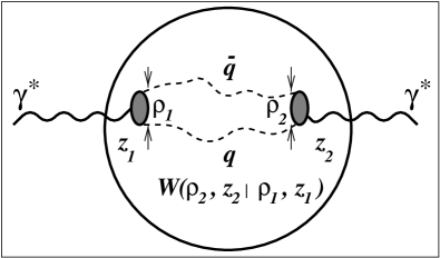
Figure 1: A cartoon for the shadowing (negative) term in (11). The Green function $W({\mbox{\boldmath$\rho$}}_{2},z_{2}|\mbox{\boldmath$\rho$}_{1},z_{1})$ results from the summation over different paths of the $q\bar{q}$ pair propagation through the nucleus.

This term, illustrated in fig. (1), is due to destructive interference between pairs created at different coordinates $z$ and contains also the contribution of the transverse motion of the pair to the coherence length. It is described by the Green function $W$ and avoids the appearance of the undefined quantity $M_{X}$. The Green function also takes the finite size of the nucleus into account.

2 Derivation of the formula

In order to derive explicit expressions for the terms in eq. (11), we start from the general expression for the cross section for the production of a $q\bar{q}$-pair,

$$d\sigma^{\gamma^{*}A} = Z_{f}^{2}\alpha_{em}\,\left|M_{fi}\right|^{2}\,\delta\left(\nu-p_{q}^{0}-p_{\bar{q}}^{0}\right)\frac{d^{3}p_{q}\,d^{3}p_{\bar{q}}}{\left(2\pi\right)^{4}\nu\,2p_{q}^{0}\,2p_{\bar{q}}^{0}}$$ (13)

$$= Z_{f}^{2}\alpha_{em}\,\left|M_{fi}\right|^{2}\,\frac{d^{2}p_{\perp,q}\,d^{2}p_{\perp,\bar{q}}\,d\lambda}{\left(2\pi\right)^{4}4\nu^{2}\,\lambda\left(1-\lambda\right)}$$

where $Z_{f}^{2}$ is the flavor charge, $\alpha_{em}=1/137$ and the matrix element is given by

$$M_{fi}=\int d^{3}r\,\Psi_{q}^{\dagger}\left(\vec{r}\right)\,\mbox{\boldmath${\alpha}$}\cdot\mbox{\boldmath$\epsilon$}\;\Psi_{\bar{q}}\left(\vec{r}\right)e^{ikz}.$$ (14)

We choose the $z$-axis to lie in direction of propagation of the photon. The photon’s momentum is denoted by $k$ and it’s energy by $\nu$, $p_{q}$ is the momentum of the quark and $p_{\bar{q}}$ the momentum of the antiquark. In eq. (13) we have introduced the energy fraction $\lambda=p_{q}^{0}/\nu$. In the ultrarelativistic case we are considering, pair production takes place predominantly in forward direction and therefore we distinguish between the longitudinal direction ($z$-direction) and the transverse directions. The longitudinal momenta are large compared to the flavor masses, $p_{z}\gg m_{f}$, and to the perpendicular momenta, $\left|\vec{p}_{\perp}\right|^{2}\sim m_{f}^{2}$. In our approximation, we keep terms of order $m_{f}/p_{z}$ only in exponentials and neglect them otherwise. All higher order terms are omitted.

Note, that the pair is created electromagnetically in a color singlet state, therefore we have the factor $Z_{f}\alpha_{em}$ in eq. (13), but we describe the with the nucleons an abelian potential $\phi\left(\vec{r}\right)$. The particles in the pair move in a potential $U\left(\vec{r}\right)$ that is a superposition of the potentials of all nucleons,

$$U\left(\vec{r}\right)=\sum\limits_{j=1}^{A}\phi\left(\vec{r}-\vec{r}_{j}\right).$$ (15)

The vector $\vec{r}_{j}$ runs over all positions of the nucleons.

The wavefunction of the quark fullfills the Dirac equations and is an eigenstate with positive energy, while the antiquark is represented by an eigenstate with negative energy,

$$\left(p_{q}^{0}-U\left(\vec{r}\right)-m_{f}{\mbox{\boldmath$\beta$}}+i\mbox{\boldmath$\alpha$}\cdot\mbox{\boldmath$\mbox{\boldmath$\nabla$}$}\right)\Psi_{q}\left(\vec{r}\right) = 0,$$ (16)

$$\left(-p_{\bar{q}}^{0}-U\left(\vec{r}\right)-m_{f}{\mbox{\boldmath$\beta$}}+i\mbox{\boldmath$\alpha$}\cdot\mbox{\boldmath$\mbox{\boldmath$\nabla$}$}\right)\Psi_{\bar{q}}\left(\vec{r}\right) = 0.$$ (17)

No interaction between the quark and the antiquark is taken into account and therefore, the two equations decouple. The wavefunction of the quark $\Psi_{q}\left(\vec{r}\right)$ contains an outgoing plane wave and an outgoing spherical wave in it’s asymptotic form, while the wavefunction of the antiquark contains an incoming spherical wave and an incoming plane wave. We transform these equations into second order equations by applying the operator $\left(p_{q}^{0}-U\left(\vec{r}\right)\right.$ $\left.+m_{f}{\mbox{\boldmath$\beta$}}-i\mbox{\boldmath$\alpha$}\cdot\mbox{\boldmath$\mbox{\boldmath$\nabla$}$}\right)$ on the first and the corresponding operator on the second equation, as described in LL . When we omit the term quadratic in the potential, we obtain

$$\left(\Delta+\left|\vec{p}_{q}\right|^{2}\!-2p_{q}^{0}U\!\!\left(\vec{r}\right)+i\mbox{\boldmath$\alpha$}\cdot\left(\mbox{\boldmath$\mbox{\boldmath$\nabla$}$}U\!\!\left(\vec{r}\right)\right)\right)\Psi_{q}\left(\vec{r}\right) = 0,$$ (18)

$$\left(\Delta+\left|\vec{p}_{\bar{q}}\right|^{2}\!+2p_{\bar{q}}^{0}U\!\!\left(\vec{r}\right)+i\mbox{\boldmath$\alpha$}\cdot\left(\mbox{\boldmath$\mbox{\boldmath$\nabla$}$}U\!\!\left(\vec{r}\right)\right)\right)\Psi_{\bar{q}}\left(\vec{r}\right) = 0.$$ (19)

The solutions may approximately be written as Furry-Sommerfeld-Maue Furry ; SM type wavefunctions,

$$\Psi_{q}\left(\vec{r}\right) = e^{i\vec{p}_{q}\cdot\vec{r}}\left(1-\frac{i\mbox{\boldmath$\alpha$}}{2p_{q}^{0}}\cdot\mbox{\boldmath$\mbox{\boldmath$\nabla$}$}\right)\,F_{q}\left(\vec{r}\right)\,u\left(p_{q},\lambda_{q}\right),$$ (20)

$$\Psi_{\bar{q}}\left(\vec{r}\right) = e^{-i\vec{p}_{q}\cdot\vec{r}}\left(1+\frac{i\mbox{\boldmath$\alpha$}}{2p_{\bar{q}}^{0}}\cdot\mbox{\boldmath$\mbox{\boldmath$\nabla$}$}\right)\,F_{\bar{q}}\left(\vec{r}\right)\,v\left(p_{\bar{q}},\lambda_{\bar{q}}\right).$$ (21)

Here, $u\left(p_{q},\lambda_{q}\right)$ is the free spinor with positive energy and polarization $\lambda_{q}$. It satisfies $\left(p_{q}\!\!\!\!\!/-m_{f}\right)u\left(p_{q},\lambda_{q}\right)=0$ and similarly $\left(p_{\bar{q}}\!\!\!\!\!/+m_{f}\right)v\left(p_{q},\lambda_{q}\right)=0$. In Dirac representation they read

$$u\left(p_{q},\lambda_{q}\right) = \sqrt{p^{0}_{q}+m_{f}}\left(\begin{array}[]{c}\displaystyle{\chi_{q}}\\ \displaystyle{\frac{\mbox{\boldmath$\sigma$}\cdot\vec{p}_{q}}{p^{0}_{q}+m_{f}}\;\chi_{q}}\end{array}\right),$$ (24)

$$v\left(p_{q},\lambda_{q}\right) = \sqrt{p^{0}_{\bar{q}}+m_{f}}\left(\begin{array}[]{c}\displaystyle{\frac{\mbox{\boldmath$\sigma$}\cdot\vec{p}_{\bar{q}}}{p^{0}_{\bar{q}}+m_{f}}\;\chi_{\bar{q}}}\\ \displaystyle{\chi_{\bar{q}}}\end{array}\right).$$ (27)

The three Pauli spin matrices are denoted by $\sigma$ and the Pauli spin state referred to the rest frame of the particle is $\chi_{q}$, or $\chi_{\bar{q}}$ respectively. This means explicitely $\vec{s}\cdot\mbox{\boldmath$\sigma$}\,\chi_{q}=\lambda_{q}\chi_{q}$ and $\vec{s}\cdot\mbox{\boldmath$\sigma$}\,\chi_{\bar{q}}=-\lambda_{\bar{q}}\chi_{\bar{q}}$ with a spin vector $\vec{s}$ normalized to unity and $\lambda_{q},\lambda_{\bar{q}}=\pm 1$. The functions $F_{q}$ and $F_{\bar{q}}$ have no spinor structure any more. They contain all dependence of the potential and have to be calculated for a given $U\left(\vec{r}\right)$. They fullfill the equations LL

$$\left(\Delta+2i\vec{p}_{q}\cdot\mbox{\boldmath$\nabla$}-2p_{q}^{0}U\left(\vec{r}\right)\right)F_{q}\left(\vec{r}\right) = 0,$$ (28)

$$\left(\Delta-2i\vec{p}_{\bar{q}}\cdot\mbox{\boldmath$\nabla$}+2p_{\bar{q}}^{0}U\left(\vec{r}\right)\right)F_{\bar{q}}\left(\vec{r}\right) = 0,$$ (29)

with boundary conditions $F\rightarrow 1$ for the quark and for the antiquark as $z\rightarrow\infty$. Note, that it is essential to take the correction proportional to $\alpha$ in eq. (20) and (21) into account, although these terms seem to be suppressed by a factor of $1/p^{0}$. It turns out, that when we calculate the matrix element of the current operator, $\left(\mbox{\boldmath$\alpha$}\cdot\mbox{\boldmath$\epsilon$}\,\right)_{fi}$, between free spinors, the large part cancels and we are left with a contribution of the same order as produced by the correction term. Thus, the terms proportional to $\alpha$ may not be neglected in the matrix element, although they give small corrections to the wave functions.

In order to remove the dependence on the transverse momenta from the phase factors in eq. (20) and (21), we rewrite the solutions in the form

$$\Psi_{q}\left(\vec{r}\right) = e^{i\left|\vec{p}_{q}\,\right|z}\left(1-\frac{i\vec{\mbox{\boldmath$\alpha$}}}{2p_{q}^{0}}\cdot\mbox{\boldmath$\nabla$}-\frac{\vec{\mbox{\boldmath$\alpha$}}_{\perp}}{2p_{q}^{0}}\cdot\vec{p}_{\perp,q}\right.$$ (30)

$$+\left.\frac{{\mbox{\boldmath$\alpha$}}_{z}}{2p_{q}^{0}}\left(\left|\vec{p}_{q}\,\right|-p_{z,q}\right)\right)\,\psi_{q}\left(\vec{r}\right)\,u\left(p_{q},\lambda_{q}\right),$$

$$\Psi_{\bar{q}}\left(\vec{r}\right) = e^{-i\left|\vec{p}_{\bar{q}}\,\right|z}\left(1+\frac{i\vec{\mbox{\boldmath$\alpha$}}}{2p_{\bar{q}}^{0}}\cdot\mbox{\boldmath$\nabla$}-\frac{\vec{\mbox{\boldmath$\alpha$}}_{\perp}}{2p_{\bar{q}}^{0}}\cdot\vec{p}_{\perp,\bar{q}}\right.$$ (31)

$$\left.+\frac{{\mbox{\boldmath$\alpha$}}_{z}}{2p_{q}^{0}}\left(\left|\vec{p}_{\bar{q}}\,\right|-p_{z,\bar{q}}\right)\right)\,\psi_{\bar{q}}\left(\vec{r}\right)\,v\left(p_{\bar{q}},\lambda_{\bar{q}}\right),$$

with

$$\psi_{q}\left(\vec{r}\right) = e^{i\vec{p}_{\perp,q}\cdot\vec{r}_{\perp}}e^{-i\left(\left|\vec{p}_{q}\,\right|-p_{z,q}\right)z}F_{q}\left(\vec{r}\right),$$ (32)

$$\psi_{\bar{q}}\left(\vec{r}\right) = e^{-i\vec{p}_{\perp,\bar{q}}\cdot\vec{r}_{\perp}}e^{i\left(\left|\vec{p}_{\bar{q}}\,\right|-p_{z,\bar{q}}\right)z}F_{\bar{q}}\left(\vec{r}\right),$$ (33)

and $\left|\vec{p}\,\right|=\sqrt{p_{0}^{2}-m_{f}^{2}}$ for the quark and the antiquark respectively. In the following, we neglect the terms containing ${\mbox{\boldmath$\alpha$}}_{z}$ in eq. (30) and (31), because they are of order $O\left(1/p^{0}_{q}p^{0}_{\bar{q}}\right)$. The functions $\psi_{q}\left(\vec{r}\right)$ and $\psi_{\bar{q}}\left(\vec{r}\right)$ will play the role of effective wave functions for the quarks.

The phase factors combine in the matrix element (14) to the minimal longitudinal momentum transfer,

$$q_{L}^{min}=k-\left|\vec{p}_{\bar{q}}\,\right|-\left|\vec{p}_{\bar{q}}\,\right|\approx\frac{Q^{2}}{2\nu}+\frac{m_{f}^{2}}{2p_{0,q}}+\frac{m_{f}^{2}}{2p_{0,\bar{q}}},$$ (34)

and we obtain

$$M_{fi}\;=\;\int d^{3}re^{iq_{L}^{min}z}$$ (35)

$$\times \left[u^{\dagger}\left(p_{q},\lambda_{q}\right)\left(\,\mbox{\boldmath$\alpha$}\cdot\mbox{\boldmath$\epsilon$}\;+\mbox{\boldmath$\alpha$}\cdot\frac{i\mbox{\boldmath$\nabla$}\left(\vec{r}_{q}\right)-\vec{p}_{\perp,q}}{2p_{q}^{0}}\,\mbox{\boldmath$\alpha$}\cdot\mbox{\boldmath$\epsilon$}\;\right.\right.$$

$$\left.\left.+\mbox{\boldmath$\alpha$}\cdot\mbox{\boldmath$\epsilon$}\,\vec{\bf\alpha}\cdot\frac{i\mbox{\boldmath$\nabla$}\left(\vec{r}_{\bar{q}}\right)-\vec{p}_{\perp,\bar{q}}}{2p_{\bar{q}}^{0}}\right)v\left(p_{\bar{q}},\lambda_{\bar{q}}\right)\right]$$

$$\times \psi_{q}^{*}\left(\vec{r}_{{q}}\right)\psi_{\bar{q}}\left(\vec{r}_{\bar{q}}\right)\Big{|}_{\vec{r}=\vec{r}_{{q}}=\vec{r}_{\bar{q}}}.$$

Here, the coherence length, $L_{c}^{max}=1/q_{L}^{min}$, comes into the game as an oscillating phase factor. However, $L_{c}^{max}$ does not depend on the transverse momenta. Their influence on the cross section is encoded in the rest of the wave functions, eq. (30) and (31). The operator $\mbox{\boldmath$\nabla$}\left(\vec{r}_{q}\right)$ acts only on the variable $\vec{r}_{q}$ and the operator $\mbox{\boldmath$\nabla$}\left(\vec{r}_{\bar{q}}\right)$ only on $\vec{r}_{\bar{q}}$. After the derivatives have been performed, the whole integrand has to be evaluated at $\vec{r}=\vec{r}_{{q}}=\vec{r}_{\bar{q}}$.

With the representation (24) , (27) we obtain after some algebra within the demanded accuracy

$$M_{fi}\;=\;\int_{-\infty}^{\infty}dze^{iq_{L}^{min}z}\int d^{2}r_{\perp}\frac{1}{\sqrt{\lambda\left(1-\lambda\right)}}$$ (36)

$$\times \chi_{q}^{\dagger}\displaystyle{\Bigg{\{}}m_{f}\mbox{\boldmath$\sigma$}\cdot\mbox{\boldmath$\epsilon$}_{T}$$

$$+i\left(1-\lambda\right)\mbox{\boldmath$\sigma$}\cdot\vec{e}_{z}\mbox{\boldmath$\epsilon$}_{T}\cdot\mbox{\boldmath$\nabla$}\left(\vec{r}_{\perp,\bar{q}}\right)+i\lambda\mbox{\boldmath$\sigma$}\cdot\vec{e}_{z}\mbox{\boldmath$\epsilon$}_{T}\cdot\mbox{\boldmath$\nabla$}\left(\vec{r}_{\perp,{q}}\right)$$

$$+\left(1-\lambda\right)\left(\vec{e}_{z}\times\mbox{\boldmath$\epsilon$}_{T}\right)\cdot\mbox{\boldmath$\nabla$}\left(\vec{r}_{\perp,{\bar{q}}}\right)-\lambda\left(\vec{e}_{z}\times\mbox{\boldmath$\epsilon$}_{T}\right)\cdot\mbox{\boldmath$\nabla$}\left(\vec{r}_{\perp,{q}}\right)$$

$$+\;2\,Q\,\lambda\left(1-\lambda\right)\Bigg{\}}\chi_{\bar{q}}$$

$$\times \psi_{q}^{*}\left(\vec{r}_{\perp,{q}},z\right)\psi_{\bar{q}}\left(\vec{r}_{\perp,\bar{q}},z\right)\Big{|}_{\vec{r}_{\perp,{q}}=\vec{r}_{\perp,\bar{q}}}.$$

Some details of the calculation can be found in OM . The unit vector in $z$-direction is denoted by $\vec{e}_{z}$. The polarisation vector $\mbox{\boldmath$\epsilon$}_{T}$ corresponds to transverse states of the $\gamma^{*}$, while the last term in the curly brackets is due to longitudinal polarisation. There are two remarkable aspect concerning this last equation. First, it does not contain any derivative with respect to $z$ any more, because of the transverse nature of the polarization vector $\mbox{\boldmath$\epsilon$}_{T}$ and of $\vec{e}_{z}\times\mbox{\boldmath$\epsilon$}_{T}$. Second, all dependence on the transverse momenta in the spinor part has cancelled.

From the eq. (28) and (29) and from the definition of $\psi$, eq. (32) and (33), we can obtain an equation for $\psi$. Assuming that these functions are only slowly varying with $z$, we omit the longitudinal part of the Laplacian and obtain

$$i\frac{\partial}{\partial z}\psi_{q}\left(\vec{r}_{\perp},z\right) = \left(-\frac{\Delta_{\perp}}{2p_{{q}}^{0}}+U\left(\vec{r}_{\perp},z\right)\right)\psi_{q}\left(\vec{r}_{\perp},z\right),$$ (37)

$$i\frac{\partial}{\partial z}\psi_{\bar{q}}\left(\vec{r}_{\perp},z\right) = \left(\frac{\Delta_{\perp}}{2p_{\bar{q}}^{0}}+U\left(\vec{r}_{\perp},z\right)\right)\psi_{\bar{q}}\left(\vec{r}_{\perp},z\right).$$ (38)

Our ansatz yields two dimensional Schrödinger equations, where the $z$-coordinate plays the role of time and the mass is given by the energy. The Laplacian $\Delta_{\perp}$ acts on the transverse coordinates only. The functions $\psi_{q}\left(\vec{r}_{\perp},z\right)$ and $\psi_{\bar{q}}\left(\vec{r}_{\perp},z\right)$ become two dimensional plane waves for $z\rightarrow\infty$, up to a phase factor that cancels in the square of the matrix element. It should be mentioned that the kinetic energy for the antiquark has a negative sign. This results from the fact that solutions of the Dirac equation with negative energy propagate backwards in time. The Laplacian in (37) and (38), account for the transverse motion of the pair in which we are especially interested. The functions $\psi_{\bar{q}}\left(\vec{r}_{\perp},z\right)$ and $\psi_{q}\left(\vec{r}_{\perp},z\right)$ in the matrix element (36) may now be expressed in terms of the Green functions for (37) and (38) and its asymptotic behaviour,

$$\psi_{q}\left(\vec{r}_{\perp,2},z_{2}\right) = \int d^{2}r_{\perp,1}\,G_{q}\left(\vec{r}_{\perp,2},z_{2}\,|\,\vec{r}_{\perp,1},z_{\infty}\right)$$ (39)

$$\times\;e^{i\vec{p}_{\perp,q}\cdot\vec{r}_{\perp,1}}e^{-i\left(\left|\vec{p}_{q}\,\right|-p_{z,q}\right)z_{\infty}},$$

$$\psi_{\bar{q}}\left(\vec{r}_{\perp,2},z_{2}\right) = \int d^{2}r_{\perp,1}\,G_{\bar{q}}\left(\vec{r}_{\perp,2},z_{2}\,|\,\vec{r}_{\perp,1},z_{\infty}\right)$$ (40)

$$\times\;e^{-i\vec{p}_{\perp,\bar{q}}\cdot\vec{r}_{\perp,1}}e^{i\left(\left|\vec{p}_{\bar{q}}\,\right|-p_{z,\bar{q}}\right)z_{\infty}}.$$

Now we use the expression for $d\sigma^{\gamma^{*}A}$, eq. (13), and with the matrix element (36) and the last two relations, we obtain

$$d\sigma^{\gamma^{*}A} = Z_{f}^{2}\alpha_{em}\;\int_{-\infty}^{\infty}dz\int_{-\infty}^{\infty}dz^{\prime}e^{iq_{L}^{min}\left(z-z^{\prime}\right)}$$ (41)

$$\int d^{2}r_{\perp}\,d^{2}\tau_{q}\,d^{2}\tau_{\bar{q}}\,\int d^{2}r_{\perp}^{\,\prime}\,d^{2}\tau_{q}^{\prime}\,d^{2}\tau_{\bar{q}}^{\prime}\,$$

$$\;\;\;\times\;\;{\cal O}\left(\vec{r}_{\perp,{q}},\vec{r}_{\perp,\bar{q}}\right)G_{q}^{*}\left(\vec{r}_{\perp,{q}},z\,|\,\mbox{\boldmath$\tau$}_{q},z_{\infty}\right)\,$$

$$\qquad\qquad G_{\bar{q}}\left(\vec{r}_{\perp,\bar{q}},z\,|\,\mbox{\boldmath$\tau$}_{\bar{q}},z_{\infty}\right)\Big{|}_{\vec{r}_{\perp}=\vec{r}_{\perp,{q}}=\vec{r}_{\perp,\bar{q}}}$$

$$\;\;\;\times\;\;{\cal O}^{*}\left(\vec{r}^{\,\prime}_{\perp,{q}},\vec{r}^{\,\prime}_{\perp,\bar{q}}\right)G_{q}\left(\vec{r}_{\perp,{q}}^{\,\prime},z^{\,\prime}\,|\,\mbox{\boldmath$\tau$}_{q}^{\,\prime},z_{\infty}\right)\,$$

$$\qquad\qquad G_{\bar{q}}^{*}\left(\vec{r}_{\perp,\bar{q}}^{\,\prime},z^{\,\prime}\,|\,\mbox{\boldmath$\tau$}_{\bar{q}}^{\,\prime},z_{\infty}\right)\Big{|}_{\vec{r}_{\perp}^{\,\prime}=\vec{r}_{\perp,{q}}^{\,\prime}=\vec{r}^{\,\prime}_{\perp,\bar{q}}}$$

$$\;\;\;\times\;\;e^{i\left(\mbox{\boldmath$\tau$}_{q}^{\,\prime}-\mbox{\boldmath$\tau$}_{q}\right)\cdot\vec{p}_{\perp,q}}\,e^{i\left(\mbox{\boldmath$\tau$}_{\bar{q}}^{\,\prime}-\mbox{\boldmath$\tau$}_{\bar{q}}\right)\cdot\vec{p}_{\perp,\bar{q}}}$$

$$\;\;\;\times\;\;\frac{d^{2}p_{\perp,q}\,d^{2}p_{\perp,\bar{q}}\,d\lambda}{\left(2\pi\right)^{4}\,\lambda^{2}\left(1-\lambda\right)^{2}4\nu^{2}}.$$

For convenience we have introduced the operator

$${\cal O}\left(\vec{r}_{\perp,{q}},\vec{r}_{\perp,\bar{q}}\right)$$ (42)

$$= \chi_{q}^{\dagger}\displaystyle{\Bigg{\{}}m_{f}\mbox{\boldmath$\sigma$}\cdot\mbox{\boldmath$\epsilon$}_{T}$$

$$+ i\left(1-\lambda\right)\mbox{\boldmath$\sigma$}\cdot\vec{e}_{z}\mbox{\boldmath$\epsilon$}_{T}\cdot\mbox{\boldmath$\nabla$}\left(\vec{r}_{\perp,\bar{q}}\right)+i\lambda\mbox{\boldmath$\sigma$}\cdot\vec{e}_{z}\mbox{\boldmath$\epsilon$}_{T}\cdot\mbox{\boldmath$\nabla$}\left(\vec{r}_{\perp,{q}}\right)$$

$$+ \left(1-\lambda\right)\left(\vec{e}_{z}\times\mbox{\boldmath$\epsilon$}_{T}\right)\cdot\mbox{\boldmath$\nabla$}\left(\vec{r}_{\perp,{\bar{q}}}\right)-\lambda\left(\vec{e}_{z}\times\mbox{\boldmath$\epsilon$}_{T}\right)\cdot\mbox{\boldmath$\nabla$}\left(\vec{r}_{\perp,{q}}\right)$$

$$+ 2\,Q\,\lambda\left(1-\lambda\right)\Bigg{\}}\chi_{\bar{q}}.$$

In order to obtain the total cross section, we integrate over $\vec{p}_{\perp,q}$ and $\vec{p}_{\perp,\bar{q}}$. The exponential factors give a $\delta$-function that enables us to perform the integrations over all the $\tau$s. Note, that ${\cal O}$ does not depend on $\tau$. We get

$$\sigma_{tot}^{\gamma^{*}A} = Z_{f}^{2}\,\frac{\alpha_{em}}{\nu^{2}}\,2\Re\int\limits_{0}^{1}\frac{d\lambda}{\lambda^{2}\left(1-\lambda\right)^{2}}$$

$$\times \;\int\limits_{-\infty}^{\infty}dz\int\limits_{z}^{\infty}dz^{\prime}e^{iq_{L}^{min}\left(z-z^{\prime}\right)}\int d^{2}r_{\perp}\,\int d^{2}r_{\perp}^{\,\prime}$$

$$\times {\cal O}\left(\vec{r}_{\perp,{q}},\vec{r}_{\perp,\bar{q}}\right){\cal O}^{*}\left(\vec{r}^{\,\prime}_{\perp,{q}},\vec{r}^{\,\prime}_{\perp,\bar{q}}\right)$$

$$\times G_{q}\left(\vec{r}_{\perp,q}^{\,\prime},z^{\,\prime}\,|\vec{r}_{\perp,q},z\right)\,$$

$$\times G_{\bar{q}}^{*}\left(\vec{r}_{\perp,\bar{q}}^{\,\prime},z^{\,\prime}\,|\vec{r}_{\perp,\bar{q}},z\right)\!\!\Big{|}_{\vec{r}_{\perp}=\vec{r}_{\perp,{q}}=\vec{r}_{\perp,\bar{q}}\,;\,\vec{r}_{\perp}^{\,\prime}=\vec{r}_{\perp,{q}}^{\,\prime}=\vec{r}^{\,\prime}_{\perp,\bar{q}}}.$$

Instead of four propagators we are left with only two, because we have used the convolution relation

$$G\left(\vec{r}_{\perp,2},z_{2}\,|\,\vec{r}_{\perp,1},z_{1}\right)$$ (44)

$$= \int d^{2}r_{\perp}\;G\left(\vec{r}_{\perp,2},z_{2}\,|\,\vec{r}_{\perp},z\right)G\left(\vec{r}_{\perp},z\,|\,\vec{r}_{\perp,1},z_{1}\right).$$

In order to derive an expression that is convenient for numerical calculations, we make use of the path-integral representation of the propagators in eq. (2). They read

$$G\left(\vec{r}_{\perp}^{\,\prime},z^{\,\prime}\,|\vec{r}_{\perp},z\right)$$

$$= \!\!\int{\cal D}\mbox{\boldmath$\tau$}\,\exp\left\{i\int\limits^{z^{\,\prime}}_{z}d\xi\left(\pm\frac{p^{0}}{2}\dot{\mbox{\boldmath$\tau$}}^{\,2}-U\left(\mbox{\boldmath$\tau$},\xi\right)\right)\right\}$$

$$\approx \!\!\int{\cal D}\mbox{\boldmath$\tau$}\,\exp\left\{i\!\int\limits^{z^{\,\prime}}_{z}\pm\frac{p^{0}}{2}\dot{\mbox{\boldmath$\tau$}}^{\,2}d\xi\right.$$

$$\left.-i\sum\limits_{j=1}^{A}\mbox{X}\left(\mbox{\boldmath$\tau$}\left(z_{j}\right)-\vec{r}_{j,\perp}\right)\vartheta\left(z^{\,\prime}-z_{j}\right)\vartheta\left(z_{j}-z\right)\right\},$$

where the upper sign corresponds to the quark and the lower to the antiquark. In this expression, $\tau$ is a function of $\xi$. The derivative with respect to $\xi$ is denoted by $\dot{\mbox{\boldmath$\tau$}}$. Obviously, the condition

$$G\left(\vec{r}_{\perp}^{\,\prime},z^{\,\prime}\,|\vec{r}_{\perp},z\right)\Big{|}_{z^{\,\prime}=z}=\delta^{(2)}\left(\vec{r}_{\perp}^{\,\prime}-\vec{r}_{\perp}\right)$$ (47)

has to be fullfilled and further it must obtain $\mbox{\boldmath$\tau$}\left(z\right)=\vec{r}_{\perp}$ and $\mbox{\boldmath$\tau$}\left(z^{\,\prime}\right)=\vec{r}_{\perp}^{\,\prime}$. In eq. (LABEL:path2), we have introduced the phase shift function $\mbox{X}\left(\mbox{\boldmath$\tau$}-\vec{r}_{j,\perp}\right)$. The step function $\vartheta\left(z\right)$ is $\mathrm{𝟎}$ for $z<0$ and $1$ for $z>0$. As mentioned before, $U$ is the superposition of all potentials of the nucleons, see eq. (15). Let $\phi$ be the potential of a single nucleon in the target. The position of the nucleon with number $j$ is denoted by the transverse vector $\vec{r}_{j,\perp}$ and the longitudinal coordinate $z_{j}$. If the range of interaction is much smaller than the distance $z^{\,\prime}-{z}$, the potential is practically zero outside the domain of integration over $\xi$ and the phase shift function is given by

$$\mbox{X}\left(\vec{r}_{\perp}-\vec{r}_{j,\perp}\right)=\int_{-\infty}^{\infty}d\xi\,\phi\left(\vec{r}_{\perp}-\vec{r}_{j,\perp},\xi-z_{j}\right).$$ (48)

We have replaced $\mbox{\boldmath$\tau$}\left(\xi\right)$ by $\mbox{\boldmath$\tau$}\left(z_{j}\right)$. This means, we use only an average value of the transverse coordinate for calculating the phase shift for scattering off a single nucleon.

The two path integrals sum over all possible trajectories of the two particles. In order to calculate the cross section for pair production in the nuclear medium, we have to average over all nucleons. We obtain with the path-integral (LABEL:path2)

$$\biggl{<}G_{q}\left(\vec{r}_{\perp,q}^{\,\prime},z^{\,\prime}\,|\vec{r}_{\perp,q},z\right)\,G_{\bar{q}}^{*}\left(\vec{r}_{\perp,\bar{q}}^{\,\prime},z^{\,\prime}\,|\vec{r}_{\perp,\bar{q}},z\right)\biggr{>}$$ (49)

$$= \left<\int{\cal D}\mbox{\boldmath$\tau$}_{q}\,\int{\cal D}\mbox{\boldmath$\tau$}_{\bar{q}}\,\exp\Biggl{\{}i\int\limits^{z^{\,\prime}}_{z}\left(\frac{p_{q}^{0}}{2}\dot{\mbox{\boldmath$\tau$}}_{q}^{\,2}+\frac{p^{0}_{\bar{q}}}{2}\dot{\mbox{\boldmath$\tau$}}_{\bar{q}}^{\,2}\right)d\xi\Biggr{.}\right.$$

$$+i\sum\limits_{j=1}^{A}\vartheta\left(z^{\,\prime}-z_{j}\right)\vartheta\left(z_{j}-z\right)$$

$$\left.\Biggl{.}\Bigl{(}\mbox{X}\left(\mbox{\boldmath$\tau$}_{\bar{q}}\left(z_{j}\right)-\vec{r}_{j,\perp}\right)-\mbox{X}\left(\mbox{\boldmath$\tau$}_{q}\left(z_{j}\right)-\vec{r}_{j,\perp}\right)\Bigr{)}\Biggr{\}}\right>,$$

with boundary conditions $\mbox{\boldmath$\tau$}_{q}\left(z\right)=\vec{r}_{\perp,q}$, $\mbox{\boldmath$\tau$}_{q}\left(z^{\,\prime}\right)=\vec{r}_{\perp,q}^{\,\prime}$, $\mbox{\boldmath$\tau$}_{\bar{q}}\left(z\right)=\vec{r}_{\perp,\bar{q}}$ and $\mbox{\boldmath$\tau$}_{\bar{q}}\left(z^{\,\prime}\right)=\vec{r}_{\perp,\bar{q}}^{\,\prime}$. The averaging procedure is similar to the one described in Glauber . We neglect all correlations between the nucleons and introduce the average nuclear density ${n_{A}}$, which is normalized to $A$, eq. (LABEL:density). Then, the whole expression may be written as an exponential, if $A$ is large enough,

$$\left<\exp\left(i\sum\limits_{j=1}^{A}\vartheta\left(z^{\,\prime}-z_{j}\right)\vartheta\left(z_{j}-z\right)\right.\right.$$ (50)

$$\Biggl{.}\Biggl{.}\Bigl{(}\mbox{X}\left(\mbox{\boldmath$\tau$}_{\bar{q}}\left(z_{j}\right)-\vec{r}_{j,\perp}\right)-\mbox{X}\left(\mbox{\boldmath$\tau$}_{q}\left(z_{j}\right)-\vec{r}_{j,\perp}\right)\Bigr{)}\Biggr{)}\Biggr{>}$$

$$= \Biggl{\{}1-\frac{1}{A}\int d^{2}s\int\limits^{z^{\,\prime}}_{z}d\xi^{\,\prime}{n_{A}}\left(\vec{s},\xi^{\,\prime}\right)\Biggl{(}1\Biggr{.}\Biggr{.}$$

$$\left.\left.-\exp\Biggl{(}i\Bigl{(}\,\mbox{X}\left(\mbox{\boldmath$\tau$}_{\bar{q}}\left(\xi^{\,\prime}\right)-\vec{s}\right)-\,\mbox{X}\left(\mbox{\boldmath$\tau$}_{q}\left(\xi^{\,\prime}\right)-\vec{s}\right)\Bigr{)}\Biggr{)}\right)\right\}^{A}$$

$$\approx \exp\Biggl{\{}-\int\limits^{z^{\,\prime}}_{z}d\xi^{\,\prime}{n_{A}}\left(b,\xi^{\,\prime}\right)\int d^{2}s\Biggr{.}$$

$$\times \left.\left(1-\exp\Biggl{(}i\Bigl{(}\,\mbox{X}\left(\mbox{\boldmath$\tau$}_{\bar{q}}\left(\xi^{\,\prime}\right)-\vec{s}\right)-\,\mbox{X}\left(\mbox{\boldmath$\tau$}_{q}\left(\xi^{\,\prime}\right)-\vec{s}\right)\Bigr{)}\Biggr{)}\right)\right\}.$$

When ${n_{A}}$ is varying fairly smoothly inside the nucleus, we can replace its dependence of $\vec{s}$, the transverse distance between the pair and the scattering nucleon, by the impact parameter $\vec{b}$, eq. (2). Since we have a short ranged interaction, it is reasonable to choose as impact parameter $\vec{b}=\left(\vec{r}_{\perp}+\vec{r}_{\perp}^{\,\prime}\right)/2$. This way we find the forward scattering amplitude for a dipole scattering off a single nucleon, see eq. (2). The corresponding cross section,

$$\sigma_{q\bar{q}}^{N}\left(\rho\right)=2\Re\int d^{2}s\left(1-\exp\Biggl{(}i\Bigl{(}\mbox{X}\left(\mbox{\boldmath$\rho$}-\vec{s}\right)-\mbox{X}\left(\vec{s}\right)\Bigr{)}\Biggr{)}\right),$$ (52)

appears as imaginary potential in the propagator. Omitting the realpart of the amplitude, which is known to be small, we finally arrive at

$$\biggl{<}G_{q}\left(\vec{r}_{\perp,q}^{\,\prime},z^{\,\prime}\,|\vec{r}_{\perp,q},z\right)\,G_{\bar{q}}^{*}\left(\vec{r}_{\perp,\bar{q}}^{\,\prime},z^{\,\prime}\,|\vec{r}_{\perp,\bar{q}},z\right)\biggr{>}$$

$$= \int{\cal D}\mbox{\boldmath$\tau$}_{q}\,\int{\cal D}\mbox{\boldmath$\tau$}_{\bar{q}}\,\exp\Biggl{\{}i\int\limits^{z^{\,\prime}}_{z}d\xi\Biggl{(}\frac{p_{q}^{0}}{2}\dot{\mbox{\boldmath$\tau$}}_{q}^{\,2}+\frac{p^{0}_{\bar{q}}}{2}\dot{\mbox{\boldmath$\tau$}}_{\bar{q}}^{\,2}\Biggr{.}\Biggr{.}$$

$$\qquad\qquad\qquad\qquad+\Biggl{.}\left.\frac{i}{2}{n_{A}}\left(b,\xi\right)\sigma_{q\bar{q}}^{N}\left(\left|\mbox{\boldmath$\tau$}_{q}-\mbox{\boldmath$\tau$}_{\bar{q}}\right|\right)\right)\Biggr{\}}.$$

Note, that all dependence on the potential of the nucleons, $\phi\left(\vec{r}\right)$, has been absorbed into $\sigma_{q\bar{q}}^{N}$. Although eq. (52) looks different for a nonabelian potential, we belief, that the formulae presented in this paper still hold, if $\sigma_{q\bar{q}}^{N}$ is taken from experiment or calculated in perturbative QCD.

It is convenient to introduce center of mass coordinates, $\mbox{\boldmath$\tau$}_{rel}=\mbox{\boldmath$\tau$}_{\bar{q}}-\mbox{\boldmath$\tau$}_{q}$ and $\mbox{\boldmath$\tau$}_{cm}=\left(1-\lambda\right)\mbox{\boldmath$\tau$}_{\bar{q}}+\lambda\mbox{\boldmath$\tau$}_{q}$, and to express the sum of the two kinetic energies as the sum of the kinetic energy of the relative motion and the center of mass kinetic energy.

$$\biggl{<}G_{q}\left(\vec{r}_{\perp,q}^{\,\prime},z^{\,\prime}\,|\vec{r}_{\perp,q},z\right)\,G_{\bar{q}}^{*}\left(\vec{r}_{\perp,\bar{q}}^{\,\prime},z^{\,\prime}\,|\vec{r}_{\perp,\bar{q}},z\right)\biggr{>}$$

$$= \int{\cal D}\mbox{\boldmath$\tau$}_{cm}\int{\cal D}\mbox{\boldmath$\tau$}_{rel}\exp\Biggl{\{}i\int\limits^{z^{\,\prime}}_{z}d\xi\left(\frac{\mu}{2}\dot{\mbox{\boldmath$\tau$}}_{rel}^{\,2}+\frac{\nu}{2}\dot{\mbox{\boldmath$\tau$}}_{cm}^{\,2}\right.\Biggr{.}$$

$$\qquad\qquad\qquad\qquad\qquad\qquad+\Biggl{.}\left.\frac{i}{2}{n_{A}}\left(b,\xi\right)\sigma_{q\bar{q}}^{N}\left(\tau_{rel}\right)\right)\Biggr{\}}$$

$$= \frac{\nu}{2\pi i\left(z^{\,\prime}-z\right)}$$

$$\times \,\exp\!\!\left(i\frac{\nu}{2}\frac{\left(\lambda\left(\vec{r}_{\perp,q}^{\,\prime}-\vec{r}_{\perp,q}\right)+\left(1-\lambda\right)\left(\vec{r}_{\perp,\bar{q}}^{\,\prime}-\vec{r}_{\perp,\bar{q}}\right)\right)^{2}}{z^{\,\prime}-z}\right)$$

$$\times \int\!\!{\cal D}\mbox{\boldmath$\tau$}_{rel}\,\exp\!\left\{\!i\int\limits^{z^{\,\prime}}_{z}d\xi\left(\frac{\mu}{2}\dot{\mbox{\boldmath$\tau$}}_{rel}^{\,2}+\frac{i}{2}{n_{A}}\left(b,\xi\right)\sigma_{q\bar{q}}^{N}\left(\tau_{rel}\right)\right)\!\!\right\}.$$

We have introduced the reduced mass

$$\frac{1}{\mu}=\frac{1}{p_{q}^{0}}+\frac{1}{p_{\bar{q}}^{0}}=\frac{1}{\nu\lambda\left(1-\lambda\right)}.$$ (56)

Since the imaginary potential depends only on the relative coordinate, the center of mass propagates freely and what remains is the effective propagator

$$W\left(\mbox{\boldmath$\rho$}^{\,\prime},z^{\,\prime}\,|\,\mbox{\boldmath$\rho$},z\right)$$

$$=\int{\cal D}\mbox{\boldmath$\tau$}_{rel}\,\exp\left\{i\int\limits^{z^{\,\prime}}_{z}d\xi\left(\frac{\mu}{2}\dot{\mbox{\boldmath$\tau$}}_{rel}^{\,2}-V_{opt}\left(b,\tau_{rel},\xi\right)\right)\right\},$$

with $\mbox{\boldmath$\rho$}^{\,\prime}=\vec{r}_{\perp,\bar{q}}^{\,\prime}-\vec{r}_{\perp,q}^{\,\prime}$ and $\mbox{\boldmath$\rho$}=\vec{r}_{\perp,\bar{q}}-\vec{r}_{\perp,q}$ and the optical potential

$$V_{opt}\left(b,\rho,z\right)=-\frac{i}{2}{n_{A}}\left(b,z\right)\sigma_{q\bar{q}}^{N}\left(\rho\right).$$ (58)

It fullfills the equation

$$\left[i\frac{\partial}{\partial z^{\,\prime}}+\frac{\Delta_{\perp}\left(\rho^{\,\prime}\right)}{2\nu\lambda\left(1-\lambda\right)}-V_{opt}\left(b,\rho^{\,\prime},z^{\,\prime}\right)\right]W\left(\mbox{\boldmath$\rho$}^{\,\prime},z^{\,\prime}\,|\,\mbox{\boldmath$\rho$},z\right)$$

$$=i\delta\left(z^{\,\prime}-z\right)\delta^{\left(2\right)}\left(\mbox{\boldmath$\rho$}^{\,\prime}-\mbox{\boldmath$\rho$}\right).\qquad$$ (59)

The propagator for the center of mass coordinate produces a $\delta$-function and thus, we obtain from eq. (2) after averaging over the medium

$$\sigma_{tot}^{\gamma^{*}A} = \frac{Z_{f}^{2}\alpha_{em}}{4\nu^{2}}\,\int d^{2}b\;2\Re\int\limits_{0}^{1}\frac{d\lambda}{\lambda^{2}\left(1-\lambda\right)^{2}}\;$$ (60)

$$\;\;\times\;\;\int\limits_{-\infty}^{\infty}dz\int\limits_{z}^{\infty}dz^{\prime}e^{iq_{L}^{min}\left(z-z^{\prime}\right)}$$

$$\;\;\times\;\;{\cal O}\!\left(\mbox{\boldmath$\rho$}\right){\cal O}^{*}\!\!\left(\mbox{\boldmath$\rho$}^{\,\prime}\right)W\!\!\left(\mbox{\boldmath$\rho$}^{\,\prime},z^{\,\prime}\,|\,\mbox{\boldmath$\rho$},z\right)\Big{|}_{\mbox{\boldmath$\rho$}^{\,\prime}=\mbox{\boldmath$\rho$}=\vec{0}},$$

with

$${\cal O}\left(\mbox{\boldmath$\rho$}\right)={\cal O}_{T}\left(\mbox{\boldmath$\rho$}\right)+{\cal O}_{L}\left(\mbox{\boldmath$\rho$}\right),$$ (61)

where the transverse part of the operator is

$${\cal O}_{T}\left(\mbox{\boldmath$\rho$}\right) = \chi_{q}^{\dagger}\displaystyle{\{}m_{f}\mbox{\boldmath$\sigma$}\cdot\mbox{\boldmath$\epsilon$}_{T}+i\left(1-2\lambda\right)\mbox{\boldmath$\sigma$}\cdot\vec{e}_{z}\mbox{\boldmath$\epsilon$}_{T}\cdot\mbox{\boldmath$\nabla$}\left(\mbox{\boldmath$\rho$}\right)$$ (62)

$$+\left(\vec{e}_{z}\times\mbox{\boldmath$\epsilon$}_{T}\right)\cdot\mbox{\boldmath$\nabla$}\left(\mbox{\boldmath$\rho$}\right)\}\chi_{\bar{q}}$$

and the longitudinal part

$${\cal O}_{L}\left(\mbox{\boldmath$\rho$}\right)=\chi_{q}^{\dagger}\displaystyle{\{}2\,Q\,\lambda\left(1-\lambda\right)\}\chi_{\bar{q}}=2\,Q\,\lambda\left(1-\lambda\right)\delta_{\lambda_{q},-\lambda_{\bar{q}}}.$$ (63)

Equation (60) is the central result of this work. It is the total cross section for production of a $q\bar{q}$-pair from a virtual photon scattering off a nucleus. We have not summed over the spins of the quark and the antiquark and not averaged over the polarizations of the photon. We have not summed over the different flavors, either. The expression for the operator ${\cal O}$, eq. (61), depends on the spin vector of the quark and the antiquark. The directions of these vectors may be fixed arbitrarily.

In order to represent the result in the form (11), we rewrite $W$ and it’s complex conjugate in an expansion. The results can be combined in the following way:

$$W\left(\mbox{\boldmath$\rho$}^{\,\prime},z^{\,\prime}\,|\,\mbox{\boldmath$\rho$},z\right)$$

$$= W_{0}\left(\mbox{\boldmath$\rho$}^{\,\prime},z^{\,\prime}\,|\,\mbox{\boldmath$\rho$},z\right)$$

$$+ i\int\limits_{z}^{z^{\,\prime}}dz_{1}\int d^{2}\rho_{1}W_{0}\left(\mbox{\boldmath$\rho$}^{\,\prime},z^{\,\prime}\,|\,\mbox{\boldmath$\rho$}_{1},z_{1}\right)\,$$

$$\;\;\times\;\;V_{opt}\left(b,\rho_{1},z_{1}\right)\,W_{0}\left(\mbox{\boldmath$\rho$}_{1},z_{1}\,|\,\mbox{\boldmath$\rho$},z\right)$$

$$- \int\limits_{z}^{z^{\,\prime}}dz_{1}\int d^{2}\rho_{1}\int\limits_{z}^{z_{1}}dz_{2}\int d^{2}\rho_{2}$$

$$\;\;\times\;\;W_{0}\left(\mbox{\boldmath$\rho$}^{\,\prime},z^{\,\prime}\,|\,\mbox{\boldmath$\rho$}_{1},z_{1}\right)\,V_{opt}^{*}\left(b,\rho_{1},z_{1}\right)\,$$

$$\;\;\times\;\;W\left(\mbox{\boldmath$\rho$}_{1},z_{1}\,|\,\mbox{\boldmath$\rho$}_{2},z_{2}\right)V_{opt}\left(b,\rho_{2},z_{2}\right)\,W_{0}\left(\mbox{\boldmath$\rho$}_{2},z_{2}\,|\,\mbox{\boldmath$\rho$},z\right).$$

Here, $W_{0}$ is the propagator corresponding to (2), when the potential is absent. The first term gives a divergent contribution, which is the wave-function renormalization for the photon. The second term leads to the first contribution in (11). The operators ${\cal O}_{T,L}$ applied to the free propagator $W_{0}$ give the light-cone wavefunctions $\Phi_{T,L}\left(\rho,\lambda\right)$, up to a constant overall factor. The third term in the above expansion is the interference term. Since this term contains the full propagator, there are no higher terms in this expansion.

As an example for further calculation, consider the integral

$$\cal{I} = -\int\limits_{-\infty}^{\infty}dz\int\limits_{z}^{\infty}dz^{\prime}e^{iq_{L}^{min}\left(z-z^{\prime}\right)}$$ (65)

$$\;\;\times\;\;\int\limits_{z}^{z^{\,\prime}}dz_{1}\int d^{2}\rho_{1}\int\limits_{z}^{z_{1}}dz_{2}\int d^{2}\rho_{2}$$

$$\;\;\times\;\;V_{opt}^{*}\left(b,\rho_{1},z_{1}\right)\,V_{opt}\left(b,\rho_{2},z_{2}\right)W_{0}\left(\mbox{\boldmath$\rho$}^{\,\prime},z^{\,\prime}\,|\,\mbox{\boldmath$\rho$}_{1},z_{1}\right)\,$$

$$\;\;\times\;\;W\left(\mbox{\boldmath$\rho$}_{1},z_{1}\,|\,\mbox{\boldmath$\rho$}_{2},z_{2}\right)W_{0}\left(\mbox{\boldmath$\rho$}_{2},z_{2}\,|\,\mbox{\boldmath$\rho$},z\right),$$

that is needed to calculate the interference part

$$\sigma_{tot}^{int} = \frac{Z_{f}^{2}\alpha_{em}}{4\nu^{2}}\,\int d^{2}b\;2\Re\int\limits_{0}^{1}\frac{d\lambda}{\lambda^{2}\left(1-\lambda\right)^{2}}$$ (66)

$${\cal O}\left(\mbox{\boldmath$\rho$}\right){\cal O}^{*}\left(\mbox{\boldmath$\rho$}^{\,\prime}\right)\;{\cal I}\,\Big{|}_{\mbox{\boldmath$\rho$}^{\,\prime}=\mbox{\boldmath$\rho$}=\vec{0}}.$$

With the new variable $\varepsilon^{2}=\lambda\left(1-\lambda\right)\,Q^{2}+m_{f}^{2}$ we find

$$q_{L}^{min}=\frac{\varepsilon^{2}}{2\nu\lambda\left(1-\lambda\right)},$$ (67)

and because of the relation

$${\left[i\frac{\partial}{\partial z^{\,\prime}}+\frac{\Delta_{\perp}\left(\rho^{\,\prime}\right)-\varepsilon^{2}}{2\nu\lambda\left(1-\lambda\right)}\right]\left(W_{0}\left(\mbox{\boldmath$\rho$}^{\,\prime},z^{\,\prime}\,|\,\mbox{\boldmath$\rho$},z\right)e^{-iq_{L}^{min}\left(z^{\,\prime}-z\right)}\right)}$$

$$=i\delta\left(z^{\,\prime}-z\right)\delta^{\left(2\right)}\left(\mbox{\boldmath$\rho$}^{\,\prime}-\mbox{\boldmath$\rho$}\right),\qquad$$ (68)

we can write the propagator in the form

$$W_{0}\left(\mbox{\boldmath$\rho$}^{\,\prime},z^{\,\prime}\,|\,\mbox{\boldmath$\rho$},z\right)e^{-iq_{L}^{min}\left(z^{\,\prime}-z\right)}$$

$$= \int\frac{d^{2}l_{\perp}}{\left(2\pi\right)^{2}}\int\limits_{-\infty}^{\infty}\frac{d\omega}{2\pi}\;\frac{\exp\left\{-i\omega\left(z^{\,\prime}-z\right)+i\vec{l}_{\perp}\cdot\left(\mbox{\boldmath$\rho$}^{\,\prime}-\mbox{\boldmath$\rho$}\right)\right\}}{{\omega-\displaystyle{\frac{\vec{l}_{\perp}^{2}+\varepsilon^{2}}{2\nu\lambda\left(1-\lambda\right)}}+i\eta}}.$$

The $+i\eta$-prescription for the pole in the complex $\omega$-plane ensures that $W_{0}\left(\mbox{\boldmath$\rho$}^{\,\prime},z^{\,\prime}\,|\,\mbox{\boldmath$\rho$},z\right)=0$ for $z>z^{\,\prime}$. Putting (2) into (65) yields after a short calculation

$$\cal{I} = -\frac{4\nu^{2}\lambda^{2}\left(1-\lambda\right)^{2}}{\left(2\pi\right)^{2}}$$

$$\;\;\times\;\;\int\limits_{-\infty}^{\infty}dz_{1}\int\limits_{-\infty}^{z_{1}}dz_{2}e^{iq_{L}^{min}\left(z_{2}-z_{1}\right)}\int d^{2}\rho_{1}\int d^{2}\rho_{2}$$

$$\;\;\times\;\;V_{opt}^{*}\left(b,\rho_{1},z_{1}\right)\,V_{opt}\left(b,\rho_{2},z_{2}\right)$$

$$\;\;\times\;\;K_{0}\!\left(\varepsilon\left|\mbox{\boldmath$\rho$}^{\,\prime}-\mbox{\boldmath$\rho$}_{1}\right|\right)W\left(\mbox{\boldmath$\rho$}_{1},z_{1}\,|\,\mbox{\boldmath$\rho$}_{2},z_{2}\right)K_{0}\!\left(\varepsilon\left|\mbox{\boldmath$\rho$}_{2}-\mbox{\boldmath$\rho$}\right|\right).$$

$K_{0}$ is the MacDonald function of zeroth order. We have used the relation

$$K_{0}\left(\varepsilon\rho\right)=\frac{1}{2\pi}\int d^{2}l_{\perp}\frac{e^{i\vec{l}_{\perp}\cdot\mbox{\boldmath$\rho$}}}{\vec{l}_{\perp}^{2}+\varepsilon^{2}}.$$ (71)

We insert (2) into (66) and calculate the contribution from the second term in the expansion (2) in a similar way. We obtain for the total cross section

$$\sigma_{tot}^{\gamma^{*}\,A} = A\,Z_{f}^{2}\,\frac{\alpha_{em}}{\left(2\pi\right)^{2}}\int\limits_{0}^{1}d\lambda\int d^{2}\rho_{1}\,\sigma^{N}_{q\bar{q}}\left(\rho_{1}\right)\,$$ (72)

$$\times \left|{\cal O}\left(\mbox{\boldmath$\rho$}\right)K_{0}\left(\varepsilon\left|\mbox{\boldmath$\rho$}-\mbox{\boldmath$\rho$}_{1}\right|\right)\Big{|}_{\mbox{\boldmath$\rho$}=\vec{0}}\right|^{2}$$

$$- Z_{f}^{2}\,\frac{\alpha_{em}}{\left(2\pi\right)^{2}}\,2\Re\int d^{2}b\int\limits_{-\infty}^{\infty}dz_{1}\int\limits_{z_{1}}^{\infty}dz_{2}$$

$$\;\;\times\;\;\int\limits_{0}^{1}d\lambda\int d^{2}\rho_{1}\int d^{2}\rho_{2}\,e^{-iq_{L}^{min}\left(z_{2}-z_{1}\right)}$$

$$\;\;\times\;\;V_{opt}^{*}\left(b,\rho_{1},z_{1}\right)\,V_{opt}\left(b,\rho_{2},z_{2}\right)$$

$$\;\;\times\;\;\left({\cal O}^{*}\left(\mbox{\boldmath$\rho$}^{\,\prime}\right)K_{0}\left(\varepsilon\left|\mbox{\boldmath$\rho$}^{\,\prime}-\mbox{\boldmath$\rho$}_{1}\right|\right)\Big{|}_{\mbox{\boldmath$\rho$}^{\,\prime}=\vec{0}}\right)$$

$$\;\;\times\;\;W\left(\mbox{\boldmath$\rho$}_{2},z_{2}\,|\,\mbox{\boldmath$\rho$}_{1},z_{1}\right)\,$$

$$\;\;\times\;\;\left({\cal O}\left(\mbox{\boldmath$\rho$}\right)K_{0}\left(\varepsilon\left|\mbox{\boldmath$\rho$}-\mbox{\boldmath$\rho$}_{2}\right|\right)\Big{|}_{\mbox{\boldmath$\rho$}=\vec{0}}\right).$$

With help of the relation

$$\mbox{\boldmath$\nabla$}\left(\mbox{\boldmath$\rho$}\right)K_{0}\left(\varepsilon\rho\right)=-\varepsilon\frac{\mbox{\boldmath$\rho$}}{\rho}K_{1}\left(\varepsilon\rho\right)$$ (73)

we find the light cone wave functions

$$\Phi_{T}\left(\varepsilon\mbox{\boldmath$\rho$}\right) = Z_{f}\,\frac{\sqrt{\alpha_{em}}}{2\pi}{\cal O}_{T}\left(\mbox{\boldmath$\rho$}\right)K_{0}\left(\varepsilon\rho\right)$$ (75)

$$= Z_{f}\,\frac{\sqrt{\alpha_{em}}}{2\pi}\Bigg{\{}m\,K_{0}\left(\varepsilon\rho\right)\,\delta_{\lambda_{q},\lambda_{\bar{q}}}\,\delta_{\lambda_{q},\lambda_{\gamma}}$$

$$+\Bigl{(}i\lambda_{q}\left(2\lambda-1\right)\mbox{\boldmath$\epsilon$}_{T}\cdot\vec{e}_{\rho}+\left(\mbox{\boldmath$\epsilon$}_{T}\times\vec{e}_{z}\right)\cdot\vec{e}_{\rho}\Bigr{)}$$

$$\;\;\times\;\;\varepsilon K_{1}\left(\varepsilon\rho\right)\delta_{\lambda_{q},-\lambda_{\bar{q}}}\Bigg{\}}$$

and

$$\Phi_{L}\left(\varepsilon\mbox{\boldmath$\rho$}\right) = Z_{f}\,\frac{\sqrt{\alpha_{em}}}{2\pi}{\cal O}_{L}\left(\mbox{\boldmath$\rho$}\right)K_{0}\left(\varepsilon\rho\right)$$ (76)

$$= Z_{f}\,\frac{\sqrt{\alpha_{em}}}{2\pi}2\,Q\,\lambda\left(1-\lambda\right)\,K_{0}\left(\varepsilon\rho\right)\,\delta_{\lambda_{q},-\lambda_{\bar{q}}}$$ (77)

We made use of the Kronecker-$\delta$. The unit vector in $\rho$-direction is denoted by $\vec{e}_{\rho}$. As spin vector we have chosen the unit vector in $z$-direction and the parameter $\lambda_{q}$ takes the value $+1$ for spin in positive $z$-direction and the value $-1$ otherwise. For the antiquark it is vice versa. For the photon, $\lambda_{\gamma}=+1$ for positive helicity and $\lambda_{\gamma}=-1$ for negative helicity. The transverse light cone wave function has one part that depends on $K_{0}$ and another part dependend on $K_{1}$, the MacDonald function of first order. Note the different spin structures of these parts. In the $K_{0}$-part, the spins of the quarks add up to the spin of the photon, but in the $K_{1}$-part of the transverse light-cone wavefunction, the spins of the quarks add to $\mathrm{𝟎}$ and the pair gets a spatial angular momentum. We finally sum over all flavors, colors, helicities and spin states and get the following expression:

$$\bar{\sigma}_{tot}^{\gamma^{*}\,A} = A\int\limits_{0}^{1}d\lambda\int d^{2}\rho\,\sigma^{N}_{q\bar{q}}\left(\rho\right)\,\left(\left|\bar{\Phi}_{T}\left(\varepsilon\rho\right)\right|^{2}+\left|\bar{\Phi}_{L}\left(\varepsilon\rho\right)\right|^{2}\right)$$ (78)

$$- \frac{3\alpha_{em}}{\left(2\pi\right)^{2}}\sum\limits_{f=1}^{N_{f}}Z_{f}^{2}\,\Re\int d^{2}b\int\limits_{-\infty}^{\infty}dz_{1}\int\limits_{z_{1}}^{\infty}dz_{2}$$

$$\;\;\times\;\;\int\limits_{0}^{1}d\lambda\int d^{2}\rho_{1}\int d^{2}\rho_{2}\,e^{-iq_{L}^{min}\left(z_{2}-z_{1}\right)}$$

$$\;\;\times\;\;{n_{A}}\left(b,z_{1}\right)\,{n_{A}}\left(b,z_{2}\right)\,\sigma^{N}_{q\bar{q}}\left(\rho_{2}\right)\,\sigma^{N}_{q\bar{q}}\left(\rho_{1}\right)$$

$$\;\;\times\;\;\Biggl{\{}\left(1-2\lambda\left(1-\lambda\right)\right)\varepsilon^{2}\frac{\mbox{\boldmath$\rho$}_{1}\cdot\mbox{\boldmath$\rho$}_{2}}{\rho_{1}\rho_{2}}K_{1}\left(\varepsilon\rho_{1}\right)K_{1}\left(\varepsilon\rho_{2}\right)\Biggr{.}$$

$$\Biggl{.}\!\!\!\!\qquad+\left(m_{f}^{2}+4Q^{2}\;\lambda^{2}\left(1-\lambda\right)^{2}\right)K_{0}\left(\varepsilon\rho_{1}\right)K_{0}\left(\varepsilon\rho_{2}\right)\Biggr{\}}$$

$$\;\;\times\;\;W\left(\mbox{\boldmath$\rho$}_{2},z_{2}\,|\,\mbox{\boldmath$\rho$}_{1},z_{1}\right).$$

Here, $\left|\bar{\Phi}_{T,L}\left(\varepsilon\rho\right)\right|^{2}$ are the absolute squares of the transverse and the longitudinal light-cone wavefunctions, summed over all flavors, see eq. (7). This form was used in first for a calculation of nuclear shadowing. Eq. (78) was for the first time suggested in a paper by Zakharov Slava1 .

Let us summarize the assumptions and approximations entering this derivation. We start from the Dirac equation with an abelian potential. We use this simplification, since we know, that all dependence of this potential will be put into the dipole cross section. Because the final result interpolates between $A\sigma_{tot}^{\gamma^{*}N}$ and eq. (9), we assume, that our results hold also for the case of a nonabelian potential.

Further, no interaction between the quark and the antiquark is taken into account and therefore, the two Dirac equations decouple. We use the Furry-Sommerfeld-Maue wavefunctions Furry ; SM that are known to be good approximations to the continous spectrum of the Dirac equation for high energies. Then we derive a two dimensional Schrödinger equation for a scalar function that may be regarded as an effective wavefunction. The $z$-coordinate plays the role of time, since the particles move almost with the velocity of light. This Schrödinger equation is solved in terms of it’s Green function. Averaging over all scattering centers in the nucleus yields an optical potential that is proportional to the total cross section for scattering a $q\bar{q}$-pair off a nucleus. We have omitted the real part of the forward scattering amplitude. All dependence on the potential is absorbed into this cross section. We propose to use the cross section as input for calculations and not the potential from which it originates. It may be taken from experimental data and is the nonperturbative input for our formulae. Analysis of hadronic cross sections PH suggests $\sigma_{q\bar{q}}^{N}(\rho)\approx C\rho^{2}$ with $C$ between $2.5$ and $3$. Note however, that we do not make any assumptions on the shape of $\sigma_{q\bar{q}}^{N}(\rho)$ in the derivation.

The averaging procedure and the summation of the multiple scattering series is similar to the one in Glauber theory Glauber and most of the approximations come in at this point. First, we neglect all correlations between the nucleons. Then, the influence of the potential is described by a phase shift function. We also assume, that we have a short ranged interaction and the pair interacts only with one nucleon at a given time. It has been demonstrated by Mueller Al , that in Born approximation the dominant contribution comes from graphs, where the $q\bar{q}$-pair interacts with the different nucleons one after another via two gluon exchange. Graphs with crossed gluon lines are suppressed. This observation justifies our summation procedure. The phase shift for scattering a particle in the pair off a single nucleon is calculated for an average value of the transverse coordinate of the particle. This means, the transverse coordinates should not vary too rapidly within a longitudinal distance of the order of the interaction range. When we want to obtain an exponential from the averaging procedure, the nuclear mass number $A$ should be large enough. Further approximations are, that both particles in the pair see the same nuclear density. We use the value of the density in the middle between the quark and the antiquark for our calculation. We also approximate the motion of the center of mass of the pair by a free motion, since the pair is scattered predominantly in forward direction.

We finally arrive at the result eq. (60). This formula allows to calculate the cross section $\sigma^{\gamma^{*}A}_{tot}$ for arbitrary polarization of the photon and the pair. However, this equation is not convenient for numerical calculations and we modify our result, introducing the light-cone wavefunctions, eq. (72). Since we are not interested in certain polarizations for a calculation of nuclear shadowing, we sum over all helicity and spin states, arriving at eq. (78).

3 Summary and conclusions

We have considered nuclear shadowing in the rest frame of the nucleus, in which the virtual photon fluctuates into a $q\bar{q}$-pair. In the preceding section we gave a detailed derivation of a formula for nuclear shadowing in DIS that accounts for both, the finite lifetime of the hadronic fluctuation and all multiple scattering terms. With this formula, eq. (78), it is possible to calculate nuclear shadowing for moderate values of $x_{B}$, $x_{B}>0.01$, where the lifetime of the fluctuation does not exceed the nuclear radius by orders of magnitude. It must be clearly emphasized, that we have only taken the $q\bar{q}$-Fock component of the photon into account and thus, the applicability of our results is restricted to values of $x_{B}$ and $Q^{2}$, where corrections from higher Fock-states of the photon, containing gluons, are not important. In particular, the structure function $F_{2}$ of the proton, calculated in our model, does not depend on $x_{B}$. In order to get the steep rise at very small $x_{B}$, one has to take higher Fock-states of the photon into account. Further, shadowing for the longitudinal cross section drops as $1/Q^{2}$ as $Q^{2}\rightarrow\infty$, since we have no gluon shadowing in our model. Adding one gluon to the $q\bar{q}$-pair would change this. This problem will be addressed in a forthcoming paper.

All assumptions summarized in the end of sec. 2 seem reasonable to us and the approximations should work as long as the nuclear mass number $A$ is not too small.

Numerical calculations first with eq. (78) show that higher order scattering terms have a significant influence on the total cross section, especially for heavy nuclei. In first , the formula for nuclear shadowing was given without derivation. This has now been made up.

The cross section $\sigma^{\gamma^{*}A}_{tot}$ is identical to the total cross section for production of a $q\bar{q}$-pair from the virtual photon in the field of the nucleus. The suppression occurs because of destructive interference between pairs created and different longitudinal coordinates within the coherence length. Thus, shadowing may be regarded as the Landau-Pomeranchuk-Migdal-effect Landau ; Migdal for pair production. This effect is the analog of the more widely known effect for bremsstrahlung and was first mentioned by Migdal Migdal for electron-positron pair production in condensed matter. However, this effect is practically not observable, because of the low density of solids. Since the density of nuclear matter is much higher, the effect occurs in $q\bar{q}$ pair production in DIS. For this reason, eq. (78) was discovered independently by Zakharov Slava1 , who considered the LPM-effect for finite size targets.

References

(1) M. Arneodo, Phys. Rept. 240 (1994) 301.
(2)
O.V. Kancheli,
Sov. Phys. JETP Lett. 18
(1973)
274.
(8) S.J. Brodsky and H.J. Lu,
Phys. Rev. Lett. 64 (1990) 1342.
(9) N.N. Nikolaev and B.G. Zakharov, Z. Phys. C49 (1991) 607.
(10) V. Barone, M. Genovese, N.N. Nikolaev, E. Pedrazzi and
B.G. Zakharov, Z. Phys. C58 (1993) 541.
(11) W. Melnitchouk and A.W. Thomas,
Phys. Lett. B317 (1993) 437.
(12) G. Piller, W. Ratzka and W. Weise,
Z. Phys. A352 (1995) 427.
(13) N.N. Nikolaev, G. Piller and B.G. Zakharov, JETP 81 (1995)
851.
(14) B.Z. Kopeliovich
and
B. Povh,
Phys. Lett. B367 (1996) 329; Z. Phys. A356
(1997)
467.
(15) V.N. Gribov, Sov. Phys. JETP 30 (1970)
709.
(16) V. Karmanov and L. Kondratyuk, Sov. Phys. JETP Lett. 18
(1973) 266.
(17) A.B. Zamolodchikov, B.Z. Kopeliovich and L.I. Lapidus,
Sov. Phys. JETP Lett. 33 (1981) 595.
(18) B.Z. Kopeliovich, J. Raufeisen and A.V. Tarasov,
Phys. Lett. B440 (1998) 151.
(19) R.J. Glauber in : Lectures in Theoretical Physics,
vol. 1, ed. W.E. Brittin and L.G. Duham, New York, Interscience, 1959.
(20) A.H. Mueller, Nucl. Phys. B335, (1990) 115.
(21)V.B. Berestetskij, E.M. Lifshitz and L.P. Pitaefskij,
Landau-Lifshitz vol. 4, part 1, Relativistic Quantum Theory, Pergamon
Press, Oxford, 1971.
(22) W.N. Furry, Phys. Rev. 46 (1934) 391.
(23) A. Sommerfeld and A.W. Maue, Ann. Phys. 22 (1935) 629.
(24) H. Olsen and L.C. Maximon, Phys. Rev. 114 (1959) 887.
(25) B.G. Zakharov, hep-ph/9807540 v2 Light-cone path integral
approach to the Landau-Pomeranchuk-Migdal effect.
(26) J. Hüfner and B. Povh, Phys. Rev. D46, (1992) 990.
(27)L.D. Landau and I.J. Pomeranchuk, Dokl. Akad. Nauk SSSR
92, (1953) 535;
92, (1953) 735. English translation in The Collected Papers of
L.D. Landau, sections 75-76, pp 586-593 Pergamon Press, (1965).