FTUAM 98/28

IFT-UAM/CSIC-98-28

Aspects of Type I String Phenomenology
L.E. Ibáñez, C. Muñoz and S. Rigolin
Departamento de Física Teórica C-XI and Instituto de Física Teórica C-XVI,
Universidad Autónoma de Madrid, Cantoblanco, 28049 Madrid, Spain.
Abstract

We study different phenomenological aspects of compact, $D=4$, $N=1$ Type IIB orientifolds considered as models for unification of the standard model and gravity. We discuss the structure of the compactification, string and unification scales depending on the different possible D-brane configurations. It is emphasized that in the context of Type I models the $M_{W}/M_{Planck}$ hierarchy problem is substantially alleviated and may be generated by geometrical factors. We obtain the effective low-energy supergravity Lagrangian and derive the form of soft SUSY-breaking terms under the assumption of dilaton/moduli dominance. We also discuss the role of anomalous $U(1)$’s and of twisted moduli in this class of theories. A novel mechanism based on the role of singularities is suggested to achieve consistency with gauge coupling unification in low string scale models.

1 Introduction

In the attempts to embed the known standard model (SM) interactions within perturbative $D=4$, $N=1$ heterotic vacua, a number of properties were generally assumed [1]. The string scale $M_{string}$ was identified essentially with the Planck mass $M_{Planck}$ and the gauge coupling unification scale $M_{X}$ was also taken to be in the vicinity of $M_{string}$. These scale identifications were not arbitrary, they were essentially dictated by the structure of the heterotic string couplings. The SM gauge group was a subgroup of either $E_{8}\times E_{8}$ or $SO(32)$ and SUSY breaking was most of the times assumed to take place by gaugino condensation in a hidden sector of the theory. A number of interesting four-dimensional $N=1$ vacua with particle content not far from that of the supersymmetric SM were found [1].

With the string theory developments of the last three years it has been realized that many of the assumptions for embedding the SM inside string theory were in fact mere artifacts of perturbative heterotic string compactifications. New vacua based on Type II and Type I strings have revealed the importance of Dirichlet D-branes [2] in the understanding of the general space of string vacua. In addition all the five known perturbative SUSY strings seem to correspond (along with $D=11$ supergravity) to particular limits of the unique underlying M-theory.

We thought we knew what the size of the string scale was: just close to $M_{Planck}$. We have now realized that we didn’t. Going away from perturbative heterotic vacua $M_{string}$ is related both to $M_{Planck}$ and the compactification scale $M_{c}$ in such a way that, in principle, $M_{string}$ may be anywhere between the weak scale and the Planck scale without any obvious contradiction with experimental facts [3]–[18]. In addition there is a much larger ambiguity in the possibilities for gauge group for $D=4$, $N=1$ vacua. Gauge groups live on the world-volume of Dp-branes and the observed SM gauge group may in principle correspond to, e.g., gauge interactions on the world-volume of 3-branes (or D(n+3)-branes with n dimensions wrapping on some compact space).

Although we are far from a complete understanding of the general structure of the new $D=4$, $N=1$ string vacua now available, it is perhaps time to try to extract some general characteristics from the known examples and see how the traditional perturbative heterotic schemes are changed. We will be interested here in compact $D=4$, $N=1$ string vacua. We are aware essentially of three avenues to construct such new vacua: 1) Type IIB $D=4$ compact orientifold models, 2) M-theory compactification on CY$\times S^{1}/Z_{2}$ and 3) F-theory compactifications on CY four-folds.

The first is the natural generalization of the toroidal heterotic orbifolds studied in the past [19, 20] to the Type IIB and Type I string theories. Their construction has developed in the last two years [21]–[29] and provides us with new perturbative vacua. Due to Type I/heterotic duality, some of these new vacua may be understood as dual to other non-perturbative heterotic vacua. This is the class of theories we are going to concentrate on in the present article. We think they are interesting because they are perturbative vacua, with which one can use standard string theory techniques, and yet provide interesting $D=4$, $N=1$ models with chiral matter. Furthermore, due to Type I/heterotic duality one expects to extract from them information about the strongly coupled regime of heterotic vacua.

We should emphasize that the model building in this kind of Type IIB orientifolds is still in its infancy and there are not yet fully realistic models. Our hope is rather trying to extract some generic features of this kind of vacua hoping that could be shared by more realistic models based on these (or other D-brane) constructions.

The content of the article is as follows. In section 2 we present a general overview of the structure of Type IIB compact $D=4$ orientifold models and of the important role played by D-branes and T-dualities in their construction. In section 3 we study the general structure of mass scales in this class of theories. After reviewing the relationship between string scale, Planck mass and compactification scale, we analyze, in subsection 3.2, different possibilities to embed the SM interactions within some Dp-brane sector with unification of coupling constants at $M_{X}=2\times 10^{16}$ GeV, as suggested by plain extrapolation of low-energy data. We find that, in order to do that within an isotropic compactification, one has to identify the unification scale $M_{X}$ with the string scale for 3-branes or 9-branes but one has to identify it with a compactification/winding scale for 5/7 branes. We also consider the possibility of embedding the SM $SU(3)_{C}$ and $SU(2)_{L}$ interactions within different types of Dp-branes. In section 4 we discuss the generic presence of very weakly coupled gauge and Yukawa interactions in models with the string scale below the Planck mass and their possible phenomenological applications.

In section 5 we discuss possible avenues for the generation of the notorious $M_{W}/M_{Planck}$ hierarchy. We argue that in the context of Type I models this problem is substantially weaker and the hierarchy may appear from purely geometrical factors.

In section 6 we extract the general form of the tree-level Kähler potential and gauge kinetic functions for this class of Type IIB orientifolds. In order to do that we make use of the T-duality symmetries which exchange among themselves the different types of Dp-branes. These symmetries also exchange dilaton with moduli so that all are essentially on equal footing. As a consequence the Kähler potential is rather symmetric under the exchange of dilaton and moduli. Furthermore the gauge kinetic function is also linear in either the dilaton $S$ or moduli $T_{i}$, depending on what Dp-brane the gauge group is originated from. All this is drastically different from the perturbative heterotic vacua in which the complex dilaton $S$ has a unique universal role.

In section 7 we use the results of section 6 in order to derive general patterns of soft SUSY-breaking terms under the assumption of dilaton/moduli SUSY breaking [30]–[34]. We emphasize that this assumption of dilaton/moduli dominance is more compelling in the D-brane scenarios where only closed string fields like $S$ and $T_{i}$ can move into the bulk and transmit SUSY breaking from one D-brane sector to some other. The soft terms obtained present explicit invariances under T-duality transformations. In certain schemes dilaton dominance is thus T-dual (and hence equivalent) to modulus dominance. As happened for similar soft terms in untwisted sectors of heterotic orbifolds, certain sum-rules among soft terms are fulfilled for any goldstino direction.

In section 8 we describe some specific issues regarding the role of pseudo-anomalous $U(1)$’s within the context of Type IIB $D=4$, $N=1$ orientifolds. In this class of theories the gauge kinetic functions have also explicit dependence on the twisted moduli fields associated to the orbifold singularities [35]. We find that in certain class of orientifolds the coefficient of that dependence is proportional to the beta function of the group considered. This suggests a new and natural way to achieve gauge coupling unification in models with low (or very low) string scale. We leave section 9 for some general final comments. We point out that, if a generic vacuum string configuration has $N=0$ brane sectors (from e.g., D-branes wrapping on non-supersymmetric cycles in the compact dimensions), will be necessary to reduce the string scale well below the Planck mass for avoiding large SUSY-breaking contributions in the ($N=1$) brane sector containing the SM.

Previous studies concerning possible phenomenological aspects of Type IIB compact orientifolds may be found in refs.[4, 36, 27, 28, 10, 12, 13, 16, 17].

2 Type IIB orientifolds, Dp-branes and T-duality

Ten-dimensional $SO(32)$ Type I string theory may be understood as an “orientifold” [37]–[42] of $D=10$, Type IIB theory under the $Z_{2}$ operation designated world-sheet parity $\Omega$ [43]. Let $(\sigma,\tau)$ be the two (space-like and time-like) world-sheet coordinates of the string. Defining the complex world-sheet coordinate $z=\exp(\tau+i\sigma)$, one then has $\Omega z={\overline{z}}$. Thus $\Omega$ transforms left-moving and right-moving vibrations of the string into each other, so that the result of a projection of IIB string under $\Omega$ is a closed unoriented string with only one, $D=10$, SUSY. In addition it turns out that the consistency of the theory (tadpole cancellation) requires the addition of twisted sectors with respect to $\Omega$. These are nothing else but Type I open strings which have to be added to the closed unoriented strings discussed above. Type IIB strings possess extended solitonic objects, Dp-branes, which have Ramond-Ramond (R-R) charges. For our purposes they may be defined as submanifolds of the full $D=10$ space where the open strings can end. They have world-volumes spanning $p+1$ dimensions with $p=-1,1,3,5,7,9$ [2] . Here we will only be concerned with the cases $p=3,5,7,9$. Open strings can only start or end on p-branes. An open string has Dirichlet boundary conditions [2] in the $9-p$ coordinates transverse to the p-brane whereas it has Neumann boundary conditions in the world-volume directions. In $D=10$ the overall cancellation of the R-R charge (equivalent to tadpole cancellation) requires the presence of 32 9-branes in the vacuum. Open strings ending on 9-branes (which means in this case anywhere) will give rise to massless $D=10$ gauge fields in the adjoint of $SO(32)$.

Type IIB, $D=4$, $N=1$ toroidal orientifolds [21]–[29] are constructed by compactifying Type IIB theory on a six-torus $T^{6}$ and further moding the theory under some discrete symmetry $G$ which acts as a discrete rotation on the compact $SO(6)$ spacetime symmetry. Thus we will have an orientifold of Type IIB on $T^{6}$ moded by $\{\Omega\times G\}$. We will consider Abelian modings with $G=Z_{N}$ or $Z_{N}\times Z_{M}$ in such a way that there is $N=1$ SUSY in four dimensions. We refer the reader to e.g. ref.[27] for a classification of possible discrete groups and further technical details. This procedure leads to overall non-vanishing R-R charges. In order to obtain consistent vacua we have to add certain types and numbers of p-branes in the vacuum in such a way that the overall charge vanishes. The type and number of p-branes required will depend on the particular orientifold considered. For $Z_{N}$ modings with odd $N$, it turns out that only 9-branes may be present. That is the case of the $Z_{3},Z_{7}$ and $Z_{3}\times Z_{3}$ orientifolds, the only ones allowed by D=4, N=1 SUSY. For even $N$, one can have both $9$-branes and/or $5$-branes. The 5-branes will have their world-volume spanning Minkowski space plus one complex compact dimension $X_{i}$, i=1,2,3. Thus there may be up to three types of 5-branes which will be denoted by $5_{i}$, i=1,2,3 depending on what complex compact coordinate is included in the 5-brane world-volume.

Instead of $\Omega$ one can use other $Z_{2}$ modings which are still consistent with $N=1$ SUSY in $D=4$. Let $O_{i}$ denote a reflection of the $i-th$ compact complex coordinate, i.e., $O_{i}(X_{j})=-X_{i}$ for $i=j$, $+X_{j}$ for $i\not=j$. In the cases discussed above one has as orientifold generators $\Omega$ and (for even $N$, in which case $G$ contains an $O_{i}O_{j}$, $i\not=j$ twist) $\Omega O_{i}O_{j}$. One can also construct consistent $D=4$, $N=1$ orientifolds using instead $(-1)^{F_{L}}\Omega O_{i}$ and $(-1)^{F_{L}}\Omega O_{i}O_{j}O_{k}$, $i\not=j\not=k\not=i$. Here $F_{L}$ is the world-sheet left-handed fermion number. In this case it turns out that tadpole cancellation conditions will require in general the presence in the vacuum of 7-branes and 3-branes respectively. There may be three different types of 7-branes, $7_{i}$, $i=1,2,3$ depending what complex dimension $X_{i}$ is transverse to the 7-brane world-volume.

Thus we see that, depending on the orientifold generators, one can deal with 3-branes, $5_{i}$-branes, $7_{i}$-branes and 9-branes. Not all types may be present simultaneously if we want to preserve $N=1$ in $D=4$. For a given $D=4$, $N=1$ vacuum with D-p-branes and D-p^′-branes one must have $(p-p^{\prime})=0,\pm 4$. Thus we can have at most either 9-branes with $5_{i}$-branes or 3-branes with $7_{i}$-branes. The number of each type of p-brane in each case is dictated by tadpole cancellation constraints. These in turn guarantee the cancellation of gauge anomalies in the effective $D=4$, $N=1$ theory. Notice that there will be a gauge group associated to each set of coincident p-branes of a given type.

T-dualities relate the different types of p-branes present in each given vacuum [2]. Consider for simplicity the 6-torus as the product of three two-tori, $T^{6}=T^{2}\times T^{2}\times T^{2}$ each with compact radii $R_{i}$, $i=1,2,3$. Now, it is well known that a duality transformation $R_{i}\rightarrow\alpha^{\prime}/R_{i}$ transforms Neumann boundary conditions on the $X_{i}$ coordinate into Dirichlet boundary conditions and vice versa [2]. This means that e.g., a 9-brane will turn into a $7_{i}$-brane and vice versa under this transformation. More generally, consider a general configuration with different types of p-branes. T-dualities will have the effect:

$$R_{1}\leftrightarrow\alpha^{\prime}/R_{1}\ \ R_{1,2}\leftrightarrow\alpha^{\prime}/R_{1,2} \ \ R_{1,2,3}\leftrightarrow\alpha^{\prime}/R_{1,2,3}$$

$$9\leftrightarrow 7_{1}\ \ 9\leftrightarrow 5_{3} \ \ 9\leftrightarrow 3$$

$$7_{2}\leftrightarrow 5_{3}\ \ 7_{1,2}\leftrightarrow 7_{2,1} \ \ 7_{1}\leftrightarrow 5_{1}$$

$$7_{3}\leftrightarrow 5_{2}\ \ 7_{3}\leftrightarrow 3 \ \ 7_{2}\leftrightarrow 5_{2}$$

$$5_{1}\leftrightarrow 3\ \ 5_{1,2}\leftrightarrow 5_{2,1} \ \ 7_{3}\leftrightarrow 5_{3}\ .$$ (2.1)

In addition one has to rescale the Type I coupling $\lambda_{I}$ as:

$$\lambda_{I}\leftrightarrow\lambda_{I}({{\alpha^{\prime}}\over{R_{1}^{2}}})\ ;\ \lambda_{I}\leftrightarrow\lambda_{I}({{{\alpha^{\prime}}^{2}}\over{R_{1}^{2}R_{2}^{2}}})\ ;\ \lambda_{I}\leftrightarrow\lambda_{I}({{{\alpha^{\prime}}^{3}}\over{R_{1}^{2}R_{2}^{2}R_{3}^{2}}})$$ (2.2)

respectively, where $\alpha^{\prime}=1/M_{I}^{2}$ with $M_{I}$ the Type I string mass. Thus given any configuration with certain distribution of p-branes in the vacuum, there are a number of equivalent configurations which are obtained from T-dualities as shown above.

Given a p-brane in a background with six compact dimensions, open strings ending on that p-brane will only have Kaluza-Klein (KK) states along the compact dimensions with Neumann boundary conditions. On the contrary, it will have winding states only in those compact directions with Dirichlet boundary conditions. This will mean for example that open strings ending on 9-branes will only have KK modes but no winding modes. On the contrary, open strings ending on 3-branes will have no KK modes but will have winding modes along all compact directions. These winding modes will correspond to open strings starting at the 3-brane, going around the torus and coming back to the 3-brane [2]. In the same way open strings ending on a $5_{i}$-brane will have KK modes on the $X_{i}$ direction but winding modes in the other two complex dimensions. The opposite happens with open strings on $7_{i}$-branes: they will have windings in the $X_{i}$ direction and KK modes in the other two. On the other hand, closed strings can have both KK and winding modes in all compact dimensions. This turns out to be important in order to figure out what is the scale related to gauge coupling unification, as we will see in the next section.

Given different sets of p-branes in a given $D=4$, $N=1$ orientifold, there will be a gauge group and charged chiral fields associated to each set of coincident (in the transverse dimensions) p-branes. They correspond to zero modes of open strings starting and ending on the same set of p-branes. In addition there will be in general chiral fields (but no gauge group) corresponding to open strings stretching between different types of p-branes like e.g. strings stretching between 9-branes and 5-branes. The different types of chiral matter fields appearing will be reviewed in section 6 (see e.g. ref.[27] for specific examples of orientifold models). In addition to gauge groups and charged chiral fields coming from open strings there are also closed strings singlet chiral fields. Among those there will be the complex dilaton $S$ and the untwisted moduli fields $T_{i}$. These are also reviewed in section 6.

Let us finally remark some points about Type I/heterotic duality. It is believed that the strongly coupled limit of $D=10$ Type I string is the heterotic $SO(32)$ string [44]. Thus one expects that the Type IIB orientifold vacua here discussed will have heterotic duals. However, these heterotic duals need not correspond to known perturbative heterotic vacua. Indeed, the orientifolds here discussed often have gauge groups with rank bigger than 20, which is impossible for perturbative heterotic vacua. Rather, the present class of models should correspond to some non-perturbative points in the heterotic moduli space.

3 D-branes, string scale and gauge coupling unification in Type I $D=4$ string vacua

3.1 D-branes, string scale and Planck mass

We will start in this section by studying the relationship between string, Planck and compactification scales in Type I $D=4$ strings of the type described above. Let us consider the relevant piece of the bosonic action of the $D=10$, $N=1$ effective Lagrangian appearing in Type I string theory:

$$S_{10}\ =\ -\int{{dx^{10}}\over{(2\pi)^{7}}}\sqrt{-g}\ (\ {{M_{I}^{8}}\over{\lambda_{I}^{2}}}\ R\ +\ {{M_{I}^{6}}\over{\lambda_{I}}}\ {1\over 4}F^{2}_{(9)}\ +\ ...\ )\ ,$$ (3.1)

where $\lambda_{I}$ is the $D=10$ Type I dilaton, $M_{I}=1/\sqrt{\alpha^{\prime}}$ is the Type I string scale and the subindex $(9)$ refers to the gauge group coming from the 32 9-branes whose world-volume fills the whole ten-dimensional space. We consider now the dimensional reduction down to four dimensions obtained by compactification on an orbifold with an underlying compact torus of the form $T^{2}\times T^{2}\times T^{2}$. The three tori are taken with volumes $(2\pi R_{i})^{2}$, $i=1,2,3$ respectively. One obtains [3, 4, 6, 10, 29]

$$S_{4}\ = \ -\int{{dx^{4}}\over{2\pi}}\sqrt{-g}\ (\ {{R_{1}^{2}R_{2}^{2}R_{3}^{2}M_{I}^{8}}\over{\lambda_{I}^{2}}}\ R\ +\ {{R_{1}^{2}R_{2}^{2}R_{3}^{2}M_{I}^{6}}\over{\lambda_{I}}}\ {1\over 4}F^{2}_{(9)}$$ (3.2)

$$+ \ \sum_{i\not=j\not=k\not=i}{{R_{i}^{2}R_{j}^{2}M_{I}^{4}}\over{\lambda_{I}}}\ {1\over 4}F^{2}_{(7_{k})}\ +\ \sum_{j=1}^{3}{{R_{j}^{2}M_{I}^{2}}\over{\lambda_{I}}}\ {1\over 4}F^{2}_{(5_{j})}\ +{1\over{\lambda_{I}}}\ {1\over 4}F_{(3)}^{2}\ +\ ...\ )\ ,$$

where we have displayed the kinetic terms for gauge bosons of the different groups which may come from the different p-branes, $p=9,7_{k},5_{j},3$. As discussed above, not all the different p-brane sectors should be present in the vacuum if we want to respect $N=1$ SUSY. The particular radius dependence of each p-brane may be obtained by noting that the gauge coupling $g_{p}$ of the vector bosons on a given p-brane is related with the Type I dilaton and the string scale as [2]

$$g_{p}^{2}\ =\ {{\lambda_{I}}\over{(2\pi)^{(2-p)}}}\ M_{I}^{(3-p)}\ .$$ (3.3)

Only for 3-branes one has that $g_{3}$ is dimensionless, while for $p=5,7,9$ one gets additional radius dependence corresponding to the fact that p-branes are wrapping on 2, 4 or 6 compact coordinates respectively. From the above equations one obtains for the gravitational coupling $G_{N}$

$$G_{N}\ =\ {1\over{M_{Planck}^{2}}}\ =\ {{\lambda_{I}^{2}M_{1}^{2}M_{2}^{2}M_{3}^{2}}\over{8M_{I}^{8}}}$$ (3.4)

and for the gauge couplings $\alpha_{p}$ for the different p-branes:

$$\alpha_{9}\ = \ {{\lambda_{I}M_{1}^{2}M_{2}^{2}M_{3}^{2}}\over{2M_{I}^{6}}}\ ;\ \alpha_{7_{i}}\ =\ {{\lambda_{I}M_{j}^{2}M_{k}^{2}}\over{2M_{I}^{4}}}\ \ ,i\not=j\not=k\not=i$$

$$\alpha_{5_{i}}\ = \ {{\lambda_{I}M_{i}^{2}}\over{2M_{I}^{2}}}\ \ ;\ \ \alpha_{3}\ =\ {{\lambda_{I}}\over 2}\ ,$$ (3.5)

where $M_{i}=1/R_{i}$. From the above formulae we observe that, unlike what happens in the heterotic case, $M_{Planck}$ and $M_{I}$ do not need to be of the same order of magnitude [3].

Consider for example the simple isotropic case in which all compactification radii are taken equal, $R_{i}=R=1/M_{c}$. Then one gets

$$M_{Planck}^{2}\ =\ {{8M_{I}^{8}}\over{\lambda_{I}^{2}M_{c}^{6}}}\ ;\ \alpha_{p}\ =\ {{\lambda_{I}}\over 2}({{M_{c}}\over{M_{I}}})^{p-3}\ ,\ p=9,7,5,3$$ (3.6)

that combined give the following relationship

$${{M_{c}^{(p-6)}}\over{M_{I}^{(p-7)}}}\ =\ {{\alpha_{p}M_{Planck}}\over{\sqrt{2}}}\ =\ 3.5\times 10^{17}\ GeV\ ,$$ (3.7)

where we have assumed $\alpha_{p}=\alpha_{X}\approx 1/24$, i.e., the unification value obtained from the extrapolation of low-energy coupling constants. Notice that in principle these equations give us a certain freedom to play with the values of the Type I string scale $M_{I}$ and the compactification scale $M_{c}$. This is to be compared to the analogous equation in the perturbative heterotic case where the relation $M_{string}=\sqrt{\frac{\alpha_{X}}{8}}M_{Planck}$ fixes the value of the string scale independently of the compactification scale. Notice also that if we want to remain in the Type I weak-coupling regime, due to relations (3.6, 3.7), one should obey the constraint

$$\lambda_{I}\ =\ 2\alpha_{p}\ ({{M_{I}}\over{M_{c}}})^{p-3}\ =\ 2\sqrt{2}{{M_{I}^{4}}\over{M_{c}^{3}M_{Planck}}}\ \leq O(1)\ .$$ (3.8)

Thus we remain in perturbation theory (in this simple isotropic case) only if $M_{I}$ is not much higher than $M_{c}$. Notice that if we insist in setting $M_{I}=M_{c}$ we get into trouble because eq.(3.7) would imply $\alpha_{p}=\sqrt{2}M_{I}/M_{Planck}$, too small a value for identifying $\alpha_{p}$ with the SM unified gauge coupling.

There are a number of natural options for the string scale $M_{I}$:

i) $M_{I}\approx M_{Planck}$. As we said, this is the option which is forced upon us in perturbative heterotic vacua [1]. In this case $M_{c}\approx M_{I}$ and gauge coupling unification should take place also about the same scale.

ii) $M_{I}\approx M_{X}$ [3]. Here $M_{X}$ is the GUT scale or the scale at which the extrapolated gauge couplings of the minimal supersymmetric standard model (MSSM) join. Numerically this is of order $10^{16}$ GeV. This corresponds (for the 3-brane case) to choices for $M_{c}$ only slightly below $M_{I}$.

iii) $M_{I}\approx\sqrt{M_{W}M_{Planck}}$. This is the geometrical intermediate scale $\approx 10^{11}$ GeV which coincides with the SUSY-breaking scale in models with a hidden sector and gravity mediated SUSY breaking in the observable sector. The interest of this choice has been recently pointed out in ref.[16] (see also ref.[13]). In this case one has (in an isotropical 3-branes situation) $M_{c}/M_{I}\approx 0.01$ and there should be precocious unification of gauge coupling constants at $M_{X}=M_{I}$.

iv) $M_{I}\approx 1$ TeV. This is the 1 TeV string scenario considered in refs.[4, 5, 6, 7, 9, 10, 15, 17, 18]. In this case it should be (in an isotropical 3-brane situation) $M_{c}/M_{I}\approx 10^{-5}$. Power-like running [45] of gauge couplings is required [7, 8] to get unification at $\approx 1$ TeV.

Many of the results we are going to discuss are independent of the scale we assume for $M_{I}$, but we will often have in mind the first three possibilities. In particular, in the next subsection we are going to consider the possibility of identifying the scale of unification of coupling constants $M_{X}\approx 2\times 10^{16}$ GeV with the string scale (possibility ii) above). On the other hand, in section 5, we will consider the generation of the $M_{W}/M_{p}$ hierarchy and argue that possibility iii) with $M_{I}\approx\sqrt{M_{W}M_{Planck}}$ allows for a natural understanding of this hierarchy [16] . This does not require the existence of extra hierarchy-generating mechanisms like gaugino condensation which seem to be necessary in possibilities i) and ii). The effective Lagrangian derived in section 6 as well as the study of soft SUSY-breaking terms induced in dilaton/moduli dominated schemes apply to the first three schemes. The novel mechanism for gauge coupling unification based on D-branes sitting close to singularities discussed in chapter 8 is in principle possible for all four schemes.

3.2 Gauge coupling unification with an isotropic compact space

The possibility of better accommodating the scale of gauge coupling unification $M_{X}=2\times 10^{16}$ GeV within Type I string theory was first considered in ref.[3]. Here we would like to consider this issue in a more systematic way for the different possibilities of embedding the SM into D-branes. We first discuss the case of an isotropic compactification with all $R_{i}=R=1/M_{c}$ and with the SM gauge group embedded in a single set of coincident p-branes of the same type (same p and same world-volume).

First we should define what are we going to call gauge coupling unification scale. We are going to assume direct unification of the $SU(3)\times SU(2)\times U(1)$ couplings without an intermediate GUT symmetry. In this context it is somewhat confusing what is the meaning of unification scale. For us it is going to be the scale above which the SM couplings join and stop running differently. This may happen because at that scale there is the string scale beyond which running no longer makes sense and tree-level string constraints between the different couplings apply. In this case one has $M_{I}=M_{X}$. Alternatively, it may be that the couplings unify at a compactification (winding) scale $M_{X}=M_{c}(M_{w})\leq M_{I}$. Both types of unification may occur depending on how we embed the SM into p-branes.

i) Embedding the SM inside 9-branes

In this case $p=9$ and, using (3.7), we have

$${{M_{c}^{3}}\over{M_{I}^{2}}}\ =\ {{\alpha_{9}M_{Planck}}\over{\sqrt{2}}}\ ;\ \lambda_{I}\ =\ 2\alpha_{9}({{M_{I}}\over{M_{c}}})^{6}\ .$$ (3.9)

Now the open strings have only Neumann boundary conditions in all dimensions and hence there are KK modes with masses of order $M_{c}$ but no open string windings. In principle one can try to identify the unification scale $M_{X}$ with either $M_{c}$ or $M_{I}$. In the first case it must be $M_{c}<M_{I}$ which implies from eq.(3.9) that $M_{X}=M_{c}>3.5\times 10^{17}$ GeV, which is too large as unification scale. The alternative possibility $M_{X}=M_{I}<M_{c}$ is consistent. Thus, in order to get $M_{X}=M_{I}=2\times 10^{16}$ GeV it is enough to choose $M_{c}=5.2\times 10^{16}$, only slightly above the string scale.

On the closed string sector there will be both KK and winding modes. The winding modes will have masses of order $M_{w}=M_{I}^{2}/M_{c}=7.7\times 10^{15}$ GeV. However they will cause no effect in the running since they are neutral objects with only gravitational interactions with charged matter. In an effective way, the charged SM particles embedded in the 9-branes will see only four dimensions below $M_{c}=5.2\times 10^{16}$ GeV whereas the closed string gravitational/moduli sector will see ten dimensions already above $M_{w}=7.7\times 10^{15}$ GeV. Thus the unification of gauge and gravitational interactions proceeds as schematically shown in Fig.1.

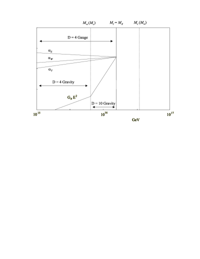
Figure 1: Running of the dimensionless gravitational coupling and gauge couplings with energy. The SM is embedded in a $9$($3$)-brane sector.

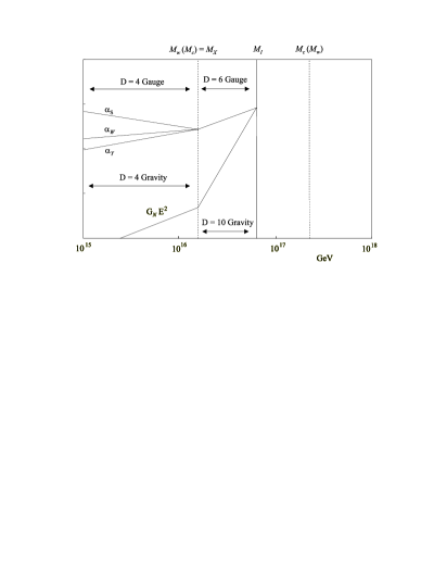
Figure 2: Running of the dimensionless gravitational coupling and gauge couplings with energy. The SM is embedded in a $7$($5$)-brane sector.

Notice that in this scenario the $D=10$ Type I dilaton remains within the perturbative regime with $\lambda_{I}=6.5\times 10^{-3}\alpha_{9}=2.7\times 10^{-4}$.

ii) Embedding the SM inside 3-branes

In this case $p=3$ and we have

$${{M_{I}^{4}}\over{M_{c}^{3}}}\ =\ {{\alpha_{3}M_{Planck}}\over{\sqrt{2}}}\ ;\ \lambda_{I}\ =\ 2\alpha_{3}\ .$$ (3.10)

This configuration is related to the one above by a T-duality transformation in all six compact dimensions [6, 29, 10]. Now open strings have Dirichlet boundary conditions in all six compact dimensions and hence have winding modes with masses of order $M_{w}=M_{I}^{2}/M_{c}$ but no KK modes. On the other hand eq.(3.10) tells us that $M_{I}>M_{c}$, otherwise $M_{I}>3.5\times 10^{17}$ GeV which is too large for unification. Thus necessarily $M_{c}<M_{I}$. One could naively say that in this case one should identify the unification scale $M_{X}$ with $M_{c}$. However this can not be because there are no open string charged KK states with masses of order $M_{c}$ but only winding states with masses $M_{w}=M_{I}^{2}/M_{c}$, higher than $M_{I}$. Thus one has actually to identify $M_{X}=M_{I}=2\times 10^{16}$ GeV, just like in the 9-brane case. In fact the physics of both cases is exactly the same, just exchanging KK modes by windings. One gets consistency with eq.(3.10) by choosing $M_{c}=7.7\times 10^{15}$ GeV, $M_{I}=2\times 10^{16}$ GeV. This is schematically shown in Fig.1. As it happens with 9-branes, although above $M_{c}$ gravity lives in ten dimensions, the SM lives on the world-volume of the 3-branes and only feels four dimensions up to the winding scale $M_{w}$. The Type I dilaton remains in the perturbative regime with $\lambda_{I}=2\alpha_{3}$.

This is qualitatively similar to the Witten scheme [3] for gauge coupling unification inside strongly coupled $E_{8}\times E_{8}$ heterotic. However, in the present case, there is an intermediate field theory regime with $D=10$ (instead of $D=5$) dimensions.

iii) Embedding the SM within 7-branes

Let us consider a set of $7_{i}$-branes with their world-volume spanning Minkowski space plus the two complex compact dimensions orthogonal to the $X_{i}$-th complex plane. We still assume for the moment an isotropic compactification of scale $M_{c}$. In this case (3.6) and (3.7) give

$$M_{c}\ =\ {{\alpha_{7}M_{Planck}}\over{\sqrt{2}}}\ ;\ \lambda_{I}\ =\ 2\alpha_{7}({{M_{I}}\over{M_{c}}})^{4}\ ,$$ (3.11)

so that, unlike previous cases, $M_{c}=3.5\times 10^{17}$ GeV is fixed and appears to be too large to be identified with the unification scale $M_{X}$. However in the present case open strings have Dirichlet boundary conditions on the $X_{i}$-th complex compact dimension and Neumann boundary conditions on the other two complex planes. Thus there will be charged winding modes with masses $M_{w}=M_{I}^{2}/M_{c}$ along the $i-th$ direction and KK modes with masses $M_{c}$ along the other two. Thus we have the hierarchy of scales $M_{w}<M_{I}<M_{c}$. Since now the winding modes are in general charged with respect to the SM interactions we must identify the unification scale $M_{X}$ with the mass of the winding modes, $M_{X}=M_{w}=M_{I}^{2}/M_{c}=2\times 10^{16}$ GeV. Thus one obtains $M_{X}=2\times 10^{16}$ GeV by taking $M_{I}=8.3\times 10^{16}$ GeV. The structure of scales is schematically shown in Fig.2.

In the present case the unification scale would coincide with the scale $M_{w}$ at which a new threshold appears corresponding to have effectively six dimensions felt by the charged fields (ten dimensions are felt by the bulk gravity fields). This interpretation is clearer in the T-dual 5-brane scheme which we discuss below. One has for the Type I dilaton coupling

$$\lambda_{I}\ =\ 2\alpha_{7}({{M_{I}}\over{M_{c}}})^{4}\ =\ 6.3\times 10^{-3}\ \alpha_{7}$$ (3.12)

thus for a realistic coupling, $\alpha_{7}=1/24$, we are well within the perturbative Type I regime.

iv) Embedding the SM within 5-branes

In this case we have

$${{M_{I}^{2}}\over{M_{c}}}\ =\ {{\alpha_{5}M_{Planck}}\over{\sqrt{2}}}\ ;\ \lambda_{I}\ =\ 2\alpha_{5}({{M_{I}}\over{M_{c}}})^{2}\ .$$ (3.13)

Let us consider one set of $5_{i}$-branes whose world-volume spans Minkowski space plus the $i$-th compact plane. Open strings will have Dirichlet boundary conditions on the two complex planes transverse to the $i$-th plane and Neumann boundary conditions in the other dimension. Thus there will be charged KK modes with masses $M_{c}$ along the $i$-th compact plane and winding modes with masses $M_{w}=M_{I}^{2}/M_{c}$ along the other two. From eq. (3.13) the winding mass is fixed to be $M_{w}=3.5\times 10^{17}$. So in this case we must identify the unification scale with the compactification scale $M_{X}=M_{c}=2\times 10^{16}$ GeV. The physical scales are much the same as the ones found for the 7-brane case. Thus correct unification is obtained by setting $M_{I}=8.3\times 10^{16}$ GeV. This is schematically shown in Fig.2. However, unlike the previous 7-brane case one finds for the Type I dilaton coupling

$$\lambda_{I}\ =\ 2\alpha_{5}({{M_{I}}\over{M_{c}}})^{2}\ =\ 35\alpha_{5}\ =\ 1.5\ .$$ (3.14)

Thus in this case we are at the border of the range of validity of the theory. One must not be surprised that in the present 5-brane case one has a larger Type I coupling whereas in the T-dual with 7-branes is much smaller (3.12). This is because under T-duality in all compact dimensions $\lambda_{I}$ transforms like $\lambda_{I}\rightarrow\lambda_{I}(M_{c}/M_{I})^{6}$ (see eq.(2.2)).

As a general conclusion one observes that assuming unification of SM interactions within a single type of p-brane, and assuming the simplest strictly isotropic compactification, one can get consistent results for all p-branes, with $p=9,3,7,5$. In the case of 9- and 3-branes one identifies the unification scale with the string scale. In the case of 7- and 5-branes one must identify it with a winding or KK threshold. In all cases one remains within Type I perturbation theory except in the case of 5-branes in which one sits close to the non-perturbative regime.

3.3 Non-isotropic compactifications

We will not attempt to make a general analysis of all possibilities. We just want to show here how departure from strict isotropy opens the way to new possibilities. Thus e.g. one can consider 9-branes (or 3-branes) scenarios in which the unification scale has to be identified with a compactification KK (winding) scale and not with the string scale $M_{I}$. Also, the 7-brane or 5-brane scenarios with isotropic compactifications considered in previous section have T-dual equivalents in which they are realized as non-isotropic compactifications within 9-branes or 3-branes. Other anisotropic scenarios in which different types of branes appear are described in the next subsection.

i) Anisotropic 9(3)-brane scenarios with a KK(winding) unification scale

We saw in previous section how unification of couplings within a 9(3)-brane with an isotropic compact space leads naturally to identify the unification scale $M_{X}$ with the string scale $M_{I}$. We will consider now a non-isotropic situation with mass scale $M_{2}$ in the first complex plane and mass scale $M_{4}$ for the other four compact dimensions. For 9-branes, using (3.4) and (3.5), we will have now

$${{M_{2}M_{4}^{2}}\over{M_{I}^{2}}}\ =\ {{\alpha_{9}M_{Planck}}\over{\sqrt{2}}}\ ;\ \lambda_{I}\ =\ 2\alpha_{9}({{M_{I}^{6}}\over{M_{2}^{2}M_{4}^{4}}})\ .$$ (3.15)

A consistent solution to these equations is obtained identifying $M_{X}=M_{I}=2\times 10^{16}$ GeV and $M_{2}=M_{4}=M_{c}=5.2\times 10^{16}$ GeV. This is the isotropic situation discussed above. Alternatively one can consider a non-isotropic hierarchy of scales $M_{2}<M_{I}<M_{4}$ and identify the unification scale with the $M_{2}$ KK scale, $M_{X}=M_{2}=2\times 10^{16}$ GeV. In this case one has to put $M_{4}^{2}=17.5M_{I}^{2}$ and the value of $M_{I}$ is only constrained above by the perturbative condition $\lambda_{I}<1$. One can obtain a physically similar scale structure by embedding the SM within 3-branes by making a T-duality transformation over all the six compact dimensions. The structure is the same but one has to replace the scales $M_{2}$ and $M_{4}$ respectively by winding scales $M_{I}^{2}/M_{2}$ and $M_{I}^{2}/M_{4}$.

ii) Anisotropic 9(3)-brane embeddings dual to 5(7)-brane isotropic embeddings

We saw how we can embed the SM couplings within a set of 5-branes with an isotropic compactification of size $M_{c}$. In that case we had $M_{X}=M_{c}=2\times 10^{16}$ GeV $<M_{I}<M_{w}$. A similar structure of physical scales can be obtained embedding the SM inside, say, 9-branes with an anisotropic compactification with $M_{2}=M_{X}$ and $M_{4}=M_{w}$. In fact both scenarios are related by a T-duality transformation along the four compact dimensions with mass scale $M_{4}$. However in the 9-brane case one finds that the Type I coupling is as small as $\lambda_{I}=2\alpha_{9}M_{I}^{6}/(M_{2}^{2}M_{4}^{4})=0.11\alpha_{9}$, well within the perturbative regime.

Something analogous can be said of the isotropic schemes with the SM embedded into 7-branes. An anisotropic compactification with the SM embedded into 3-branes can be found which gives rise to the same pattern of scales and perturbative unification.

3.4 Embedding $SU(3)$ and $SU(2)$ within different sets of p-branes

It is a plausible situation to assume that the $SU(3)$ and the $SU(2)$ groups of the SM could come from different sets of p-branes [36, 10]. By different sets we mean p-branes whose world-volume is not identical. In particular, notice that the SM contains particles (the left-handed quarks) transforming both under $SU(3)$ and $SU(2)$. That means that there must be some overlap of the world-volumes of both sets of p-branes. Thus e.g., one cannot put $SU(3)$ inside a set of 3-branes and $SU(2)$ within another set of parallel 3-branes on a different point of the compact space since then there would be no massless modes corresponding to the exchange of open strings between both sets of brane which could give rise to the left-handed quarks. Thus we need to embed $SU(3)$ inside a p-brane and $SU(2)$ within a q-brane in such a way that their corresponding world-volumes have some overlap.

Let us first consider what is the relationship between coupling constants for gauge groups coming from p-,q-branes. From eq.(3.6) one has for an isotropic compactification with compact scale $M_{c}$:

$$\alpha_{p}\ =\ \alpha_{q}({{M_{I}}\over{M_{c}}})^{q-p}$$ (3.16)

Now, if we want to preserve $N=1$ SUSY one has $q-p=0,\pm 4$. Thus, for an isotropic compactification one naturally has $\alpha_{7_{i}}=\alpha_{7_{j}}$ and $\alpha_{5_{i}}=\alpha_{5_{j}}$ whereas $\alpha_{9}=\alpha_{5_{i}}(M_{c}/M_{I})^{4}$ and $\alpha_{3}=\alpha_{7_{i}}(M_{I}/M_{c})^{4}$. In order to embed the $SU(3)$ and $SU(2)$ gauge factors inside different brane sectors the possibilities are (p,q) = $(9,5_{i})$, $(7_{i},7_{j})$, $(5_{i},5_{j})$, $(3,7_{i})$ with $i\not=j$. Thus one naturally obtains $\alpha_{S}=\alpha_{W}$ for the cases (p,q) = $(7_{i},7_{j})$, $(5_{i},5_{j})$. In the other two cases one will have $\alpha_{S}/\alpha_{W}=(M_{c}/M_{I})^{\pm 4}$ and thus one of the couplings will be suppressed compared to the other one unless $M_{c}=M_{I}$. But in such a case, due to (3.7), one is forced to have $M_{I}=3.5\times 10^{17}$ GeV, too large a value for unification.

In fact if one goes beyond the isotropic scale, a certain amount of fine-tuning is required in all cases in order to obtain $\alpha_{S}=\alpha_{W}$. Indeed, if the compact scale in the i-th direction is denoted by $M_{i}$ one has in this more general case (see eq.(3.5)):

$$\alpha_{5_{i}}\ =\ \alpha_{5_{j}}({{M_{i}}\over{M_{j}}})^{2}\ \alpha_{7_{i}}\ =\ \alpha_{7_{j}}({{M_{j}}\over{M_{i}}})^{2}$$ ;

$$\alpha_{7_{i}}\ =\ \alpha_{3}({{M_{j}M_{k}}\over{M_{I}^{2}}})^{2} \alpha_{9}\ =\ \alpha_{5_{i}}({{M_{j}M_{k}}\over{M_{I}^{2}}})^{2}$$ ; (3.17)

where $i\not=j\not=k\not=i$. Thus even in the cases (p,q) = $(7_{i},7_{j})$, $(5_{i},5_{j})$ one has to adjust $M_{i}=M_{j}$ to a good precision in order to have $\alpha_{S}=\alpha_{W}$.

On the other hand one would in principle expect that the embedding into different sets of p-branes would allow for new gauge coupling unification possibilities [10] if one is prepared to accept some degree of fine-tuning of the compactification scales. For example one can consider the $SU(3)$ and $SU(2)$ gauge couplings crossing at $M_{X}=2\times 10^{16}$ GeV and then diverging at higher energies. One could have $M_{i}\approx M_{I}=3.5\times 10^{17}$ GeV. If $SU(3)$ and $SU(2)$ come from different sets of 7-branes $7_{i}$, $7_{j}$, a small difference between $M_{i}$ and $M_{j}$ is able to explain the fact that at $M_{I}$ the running gives $\alpha_{W}>\alpha_{S}$. Something analogous may be done in the $(5_{i},5_{j})$ scheme. However there are some difficulties with the unification of the hypercharge $U(1)_{Y}$, as we now explain.

In Type IIB orientifold models, and in general on the world-volume of D-branes, $SU(n)$ groups come along with a $U(1)$ factor so that indeed we are dealing with $U(n)$ groups in which both $SU(n)$ and $U(1)$ share the same coupling constant. Assume that the $U(1)_{Y}$ is embedded into $U(3)\times U(2)$ in such a way that the left-handed quarks (belonging to the p-(q-)brane sector) have the standard hypercharge assignment. Then one obtains:

$${1\over{\alpha_{Y}}}\ =\ {2\over 3}{1\over{\alpha_{S}}}\ +\ {1\over{\alpha_{W}}}$$ (3.18)

In particular one has the expression:

$$\sin^{2}\theta_{W}\ =\ {{3/8}\over{3/4+\alpha_{W}/4\alpha_{S}}}$$ (3.19)

Thus for $\alpha_{S}=\alpha_{W}$ one obtains the standard GUT normalization for couplings, $\alpha_{Y}=3/5\alpha_{W}$ and $\sin^{2}\theta_{W}=3/8$.

Notice that for $\alpha_{W}>\alpha_{S}$ (as happens if the couplings keep on running beyond $M_{X}=2\times 10^{16}$ GeV), one has $\sin^{2}\theta_{W}<3/8$. This goes in the wrong direction for unification of the three coupling constants (notice that at $M_{I}>M_{X}$ it should be $5/3\alpha_{Y}>\alpha_{W}$). Thus, even if we adjust appropriately the $M_{i}$ in order to match $\alpha_{W}>\alpha_{S}$ at $M_{I}=3.5\times 10^{17}$ GeV, the value of $\sin^{2}\theta_{W}$ at that scale is going to be too small to be consistent with low-energy data. One can consider the possibility of $U(1)_{Y}$ not being completely included in $U(3)\times U(2)$ but having some component in other brane sector. In such a case the equality sign in eq.(3.18) should be replaced by an inequality $>$, leading to an even smaller weak angle.

We thus conclude that embedding $SU(3)$ and $SU(2)$ inside different type of p-branes and trying to maintain $M_{I}\approx M_{i}\approx 3.5\times 10^{17}$ GeV do not lead to consistent low-energy results for $\sin^{2}\theta_{W}$, even accepting some degree of fine-tuning. On the other hand the appropriate GUT relationships $\alpha_{S}=\alpha_{W}=5/3\alpha_{Y}$ are obtained if we embed $SU(3)$ and $SU(2)$ into either a set of $(5_{i},5_{j})$ or $(7_{i},7_{j})$ branes with all $M_{i}=M_{c}=2\times 10^{16}$ GeV in the first case and $M_{I}^{2}/M_{c}=2\times 10^{16}$ GeV in the second. In that case the structure of mass scales would be analogous to those we found for the case of embedding the SM within a single $5$-brane or $7$-brane sector, choosing $M_{I}=8\times 10^{16}$ GeV. The two cases are however not equivalent since the world-volumes of the $5$-branes or $7$-branes in which $SU(3)$ and $SU(2)$ live in the present case are now different.

4 Micro gauge/Yukawa interactions

Eq.(3.17) shows that there may potentially appear gauge couplings widely different if there are large differences between the compactification scales and/or string scale. Consider e.g., a general situation with one set of 3-branes plus sets of $7_{i}$-branes of the different types $i=1,2,3$. Then the corresponding gauge couplings will be related by:

$$g_{7_{i}}\ =\ g_{3}({{M_{j}M_{k}}\over{M_{I}^{2}}})\ ;\ g_{7_{i}}\ =\ g_{7_{j}}({{M_{j}}\over{M_{i}}})\ .$$ (4.1)

If all scales $M_{i}$ are of the same order of magnitude and all not far away from the string scale $M_{I}$, as mostly considered in the previous chapter, the different gauge couplings will have similar sizes. However in schemes with large compactification radii very small gauge couplings naturally appear [10].

Consider first an isotropic case with $M_{i}=M_{c}$. Depending on our choice for the string scale one has:

i) $M_{I}=1$ TeV

If one assumes $M_{c}\approx 10MeV$ as in isotropic schemes with $M_{I}=1$ TeV, one gets $g_{7_{i}}=10^{-10}g_{3}$. Thus in a scheme with a 1 TeV string scale and the SM sitting on 3-branes, the gauge interactions coming from 7-branes would appear to be very much suppressed like $(M_{c}/M_{I})^{4}$. They may be even more suppressed in a non-isotropic scenario with two dimensions with inverse size of order $10^{-3}$ eV and the other two slightly below 1 TeV [5, 6]. In this case eq.(4.1) yields $g_{7_{i}}=10^{-15}g_{3}$. There is however a generic problem concerning the possibility of these micro-gauge interactions in $M_{I}=1$ TeV scenarios. Indeed, if the compactification scales are as low as 10 MeV or even smaller, the 7-branes wrapping around those compact dimensions will give rise to open string KK modes which (unlike the closed string ones) will in general couple to the visible 3-brane sector. Thus, unless one finds a mechanism to hide these 7-brane sectors and to forbid the presence of massless chiral fields in the (3-7) open string sector, this micro gauge interactions do not seem viable.

More generally, having 7-branes along with 3-branes present in a 1 TeV scenario will in general be dangerous unless the four compact dimensions around which the 7-branes are wrapping are close to the TeV scale. In this way the open string KK states will be sufficiently heavy. These requires the other two compact dimensions to have a scale of order $10^{-3}$ eV in order to reproduce the usual Planck mass. But then the gauge interactions associated to these 7-branes are not going to be suppressed since they have couplings proportional to the compact scales of wrapped dimensions. In conclusion, in 1 TeV schemes, micro-gauge interactions due to 7-branes wrapping on large dimensions do not seem viable. This is unfortunate because in these 1 TeV schemes the stability of the proton is particularly problematic. It has been proposed [5, 6] that some $U(1)_{B}$ field living in the bulk and gauging baryon number could forbid fast proton decay. On the other hand it is not obvious how to get such bulk $U(1)$’s in the orientifold scheme. A natural alternative would have been a micro-gauged $U(1)_{B}$ living on a 7-brane with its world-volume including two large compact dimensions. We have just seen this does not look viable.

ii) $M_{I}=10^{11}$ GeV

This is the case studied in ref.[16] (see also next section). In this case one has $M_{c}=10^{9}$ GeV and one gets $g_{7_{i}}=10^{-4}g_{3}$. Thus if the SM is contained in a 3-brane sector, the gauge interactions on the 7-brane world-volume will be of the typical size of first generation Yukawa couplings. Smaller gauge couplings may be obtained in non-isotropic configurations. Indeed if e.g. the compact dimensions $X_{2,3}$ have sizes $M_{2}\approx M_{3}\approx M_{I}$ one can have $M_{1}$ as small as $10^{5}$ GeV and still maintain the correct Planck mass. Then we would get micro-gauge interactions for gauge groups in the $7_{2}$ and $7_{3}$ world-volumes with $g_{7_{2,3}}=10^{-6}g_{3}$.

iii) $M_{I}=2\times 10^{16}$ GeV

This is the case put forward in ref.[3]. In this case one has $M_{c}\approx 8\times 10^{15}$ GeV and $g_{7_{i}}\approx g_{3}/4$. Even in this case the gauge couplings of gauge interactions coming from the 7-brane sectors are smaller than the 3-brane ones.

Notice that the different type of branes map under Type I/heterotic duality into perturbative and non-perturbative gauge groups. Thus, from the heterotic point of view, what we find is that the e.g., non-perturbative gauge couplings should be much smaller than the perturbative ones as long as there are some dimensions which are relatively large, like in all three schemes reviewed above.

These micro-gauge interactions could have some interesting applications in order to generate some flavor structure in specific models. In addition to the micro gauge interactions there will be in general accompanying micro-Yukawa couplings of the same size. It is tempting the idea of associating the first (and perhaps the second) SM generation Yukawa couplings to these micro-Yukawa couplings. This idea is however difficult to realize due to the micro-gauge interactions which come along which would give rise to departures from universality in the SM gauge interactions. More concrete semi-realistic models would be needed to test this idea.

5 The generation of the $M_{W}/M_{Planck}$ hierarchy

Given the new possibilities for mass scales present in $D=4$, $N=1$ Type I string vacua, it is worth revisiting also the SUSY-breaking scales as well as the generation of the $M_{W}-M_{Planck}$ hierarchy.

The orthodox scenario for the generation of the $M_{W}/M_{Planck}$ hierarchy in perturbative heterotic vacua is the assumption of the existence of a hidden sector in the theory which couples only gravitationally to the usual particles of the SM. Indeed in perturbative heterotic vacua there are often this kind of hidden sectors which usually also involve gauge interactions [1]. A natural possibility is to assume that the gauginos of the hidden sector may condense at a scale $\Lambda\approx 10^{13}$ GeV so that SUSY is broken and the gravitino gets a mass $m_{3/2}\approx\Lambda^{3}/M_{Planck}^{2}\approx M_{W}$.

The existence of hidden sectors is equally natural within Type I vacua. For example, one can consider two separate sets of parallel p-branes ($p<9$) , one set containing the SM and the other the hidden sector interactions. If the positions of these p-branes in the transverse space are different, there will be no massless states charged under both p-brane groups. In the case of 9-branes the same effect is obtained by adding discrete Wilson lines to the model. In what follows we will consider an ideal situation of the above type in which we have a set of p-branes with unbroken $N=1$ SUSY containing the SM and a distant (hidden) set of parallel p-branes in which SUSY is somehow broken and one has $N=0$. Now, the SM does not feel directly the breaking of SUSY taking place in the hidden p-brane sector. The effects of SUSY-breaking can only be transmitted through the closed string sector fields, which are the only ones that can move into the bulk and couple to both p-brane sectors. Thus the SUSY breaking felt by the SM fields will be suppressed by $M_{Planck}$ powers. In particular one expects that the soft SUSY-breaking terms felt in this visible sector will be of order:

$$M_{W}\ \approx\ m_{3/2}\ \approx\ {{F}\over{M_{Planck}}}\ \approx\ {{\xi M_{ss}^{2}}\over{M_{Planck}}}\ ,$$ (5.1)

where $F$ denotes the SUSY-breaking auxiliary field and $M_{ss}$ is the relevant physical scale in the hidden sector. Here $\xi$ is just a dimensionless fudge factor whose size we will discuss below. It may be of order one or hierarchically small depending on how the $N=0$ hidden theory is originated. Combining (5.1) with (3.7) one has:

$${{M_{W}}\over{M_{Planck}}}\ =\ \xi{{\alpha_{p}^{2}}\over{2}}\ M_{ss}^{2}\frac{M_{I}^{2(p-7)}}{M_{c}^{2(p-6)}}\ ,$$ (5.2)

with $p$=9,7,5,3. Depending on the relative values of $M_{I}$ and $M_{c}$ and which type of p-brane is being considered, the relevant physical scale in the hidden sector should be identified with a)$M_{ss}=M_{I}$ , b) $M_{ss}=M_{c}$ or c) $M_{ss}=M_{I}^{2}/M_{c}$ (a winding scale).

i) Case with $M_{ss}=M_{I}$

Let us start by assuming the case in which the relevant scale of the hidden sector is $M_{ss}=M_{I}$. Now, let us consider for simplicity an overall compactification scale $M_{c}$. Using (5.2) one obtains:

$${{M_{W}}\over{M_{Planck}}}\ =\ \xi{{\alpha_{p}^{2}}\over{2}}\ ({{M_{I}}\over{M_{c}}})^{2(p-6)}\ .$$ (5.3)

This equation is remarkable since it shows us that it is in principle possible to generate a $M_{W}-M_{Planck}$ hierarchy even for $\xi\approx 1$ without invoking any hierarchically suppressed non-perturbative effect like e.g., gaugino condensation. This is the possibility discussed in [16]. Indeed, consider first the $p=3$ case. In this case one has

$${{M_{W}}\over{M_{Planck}}}\ =\ \xi{{\alpha_{3}^{2}}\over{2}}\ ({{M_{c}}\over{M_{I}}})^{6}$$ (5.4)

If one has $M_{I}/M_{c}\approx 160$ and $\alpha_{3}=1/24$ one indeed obtains the desired hierarchy $M_{W}/M_{Planck}=10^{-16}$ even for $\xi\approx 1$. This small ratio arises from a combination of geometrical factors which amplify the modest input hierarchy $M_{I}/M_{c}$. The final structure of scales would be $M_{c}:M_{I}:M_{I}^{2}/M_{c}=10^{9}:10^{11}:10^{13}$ GeV. The argumentation works equally well for the $p=9$ case in which a similar formula is obtained with the replacements $\alpha_{3}\leftrightarrow\alpha_{9}$ and $M_{I}/M_{c}\leftrightarrow M_{c}/M_{I}$. In this case the input hierarchy would be the inverse, $M_{c}/M_{I}\approx 160$.

For this scheme to work one has to be sure that we remain within Type I perturbation theory. This requires $\lambda_{I}=2\alpha_{p}(M_{I}/M_{c})^{(p-3)}<1$. This is the case indeed for 3-branes and 9-branes.

In the case of 7-branes (and their T-duals the 5-branes) the situation is a bit different. For both cases remaining in perturbation theory requires $M_{I}\leq M_{c}$. Then the winding scale $M_{I}^{2}/M_{c}$ will actually be lighter than the string scale $M_{I}$ so we rather take $M_{ss}=M_{I}^{2}/M_{c}$ instead of $M_{ss}=M_{I}$. Thus we turn now to this possibility.

ii) Case with $M_{ss}=M_{I}^{2}/M_{c}$

This case corresponds to a hidden p-brane sector in which the lightest cut-off scale correspond to charged winding modes with masses $M_{I}^{2}/M_{c}$ rather than the string excitations with masses of order $M_{I}$. Notice that this may be the case only for $p=3,5,7$ but not for 9-branes which have no charged winding modes. Now one parametrizes $F=\xi(M_{I}^{2}/M_{c})^{2}$ and using (5.2) obtains:

$${{M_{W}}\over{M_{Planck}}}\ =\ \xi{{\alpha_{p}^{2}}\over{2}}\ ({{M_{I}}\over{M_{c}}})^{2(p-5)}$$ (5.5)

Note that no hierarchy is obtained for 5-branes (for $\xi\approx 1$). Furthermore, in the case of 3-branes obtaining a suppression would require $M_{c}<<M_{I}$ in which case one has $M_{I}<<M_{I}^{2}/M_{c}$ and we rather identify $M_{ss}=M_{I}$, as in the previous paragraph. Finally, one naturally obtains a suppression of $M_{W}$ versus $M_{Planck}$ in the case of 7-branes. By choosing $M_{I}/M_{c}\approx 10^{-3}$ one obtains the appropriate hierarchy even for $\xi\approx 1$. In the case of 7-branes one has $M_{c}=\alpha_{7}M_{Planck}/\sqrt{2}$ hence we finally would have scales of order $M_{I}^{2}/M_{c}:M_{I}:M_{c}=10^{11}:10^{14}:10^{17}$ GeV.

iii) Case with $M_{ss}=M_{c}$

This case corresponds to a hidden p-brane sector in which the lightest cut-off scale correspond to KK modes with masses $M_{c}$ rather than the string excitations with masses of order $M_{I}$. Notice that this may be the case only for $p=5,7,9$ but not for 3-branes which have no charged KK modes. We now have $F=\xi M_{c}^{2}$ and using (5.2) one gets:

$${{M_{W}}\over{M_{Planck}}}\ =\ \xi{{\alpha_{p}^{2}}\over{2}}\ ({{M_{I}}\over{M_{c}}})^{2(p-7)}$$ (5.6)

Note that no hierarchy is obtained for 7-branes (for $\xi\approx 1$). Furthermore in the case of 9-branes obtaining a suppression would require $M_{I}<<M_{c}$. But in that case we rather identify $M_{ss}=M_{I}$ as in the first paragraph. Finally, one naturally obtains a suppression of $M_{W}$ versus $M_{Planck}$ in the case of 5-branes. By choosing $M_{I}/M_{c}\approx 10^{3}$ one obtains the appropriate hierarchy even for $\xi\approx 1$. This scheme is really T-dual to the previous one and we finally would have scales of order $M_{c}:M_{I}:M_{I}^{2}/M_{c}=10^{11}:10^{14}:10^{17}$ GeV.

In summary, we have shown that in Type I, $D=4$ vacua the hierarchy problem is ameliorated by the presence of geometrical factors of the form $\alpha^{2}(M_{I}/M_{c})^{\pm 6}$ or $\alpha^{2}(M_{I}/M_{c})^{\pm 4}$ depending on the cases. These geometrical factors may in fact explain the whole of the $M_{W}/M_{Planck}$ hierarchy ($\xi=1$) in terms of modest initial hierarchies $M_{I}/M_{c}\approx 10^{\pm 2}$.

If all of the hierarchy is explained in that way, one has to give up standard gauge coupling unification at $2\times 10^{16}$ GeV as discussed in section 3 . Indeed, in principle the mass scale $M_{ss}$ discussed here corresponds to the scale one expects coupling constants to join, thus one would expect $M_{X}=M_{ss}$. Thus e.g., if one takes $M_{I}=\sqrt{M_{W}M_{Planck}}$ and one assumes $\xi\approx 1$ the unification scale should be identified with $M_{ss}\approx 10^{11}$ GeV. In ref.[16] it was shown how the addition of some extra charged matter fields beyond those of the MSSM can give rise to precocious gauge coupling unification at $10^{11}$ GeV. Furthermore we will show in section 8 a novel mechanism by which gauge coupling unification can be understood if the observable 3-branes sit close to a repaired singularity.

5.1 Gaugino condensation

A natural possibility often considered to generate a hierarchically small $\xi$ is gaugino condensation. Let us assume that there is gaugino condensation in the hidden p-brane sector. In this case one expects the generation of an auxiliary field:

$$F\ =\ {{\Lambda^{3}}\over{M_{Planck}}}\ \approx e^{-3/2\beta\alpha_{p}}\times{{M_{ss}^{3}}\over{M_{Planck}}}$$ (5.7)

and hence comparing with the formulae in previous section one has

$$\xi\ =\ e^{-3/2\beta\alpha_{p}}\times{{M_{ss}}\over{M_{Planck}}}\ .$$ (5.8)

Here $\beta$ is the beta-function coefficient of the condensing gauge group which has coupling $\alpha_{p}$. Coming back to the three possibilities considered above for the value of the cut-off scale $M_{ss}$ i.e., $M_{ss}=M_{I},M_{I}^{2}/M_{c},M_{c}$ one obtains

$$\xi\ =\ e^{-3/2\beta\alpha_{p}}{{\alpha_{p}}\over{\sqrt{2}}}({{M_{I}}\over{M_{c}}})^{(p-a)}$$ (5.9)

with $a=6,7,5$ respectively for the three $M_{ss}$ possibilities. Thus, for example for the case of 3-branes which have $M_{ss}=M_{I}$, one gets a hierarchy:

$${{M_{W}}\over{M_{Planck}}}\ =\ e^{-3/2\beta\alpha_{3}}{{\alpha_{3}^{3}}\over{2\sqrt{2}}}\ ({{M_{c}}\over{M_{I}}})^{9}\ .$$ (5.10)

One can now simultaneously impose correct gauge coupling unification in the visible 3-brane sector with $M_{I}=M_{ss}=2\times 10^{16}$ GeV, as we described in section 3. In this case one has $M_{c}=7.7\times 10^{15}$ GeV so that, for $\alpha_{3}=1/24$ one gets $M_{W}/M_{Planck}=10^{-8}\times\exp(-3/2\beta\alpha_{3})$.

6 Effective low-energy Lagrangian in $D=4$ $N=1$ compact orientifold models

In this section we will extract the structure of the Kähler potential corresponding to the untwisted closed string fields (dilaton and moduli) as well as that of the charged chiral fields coming from the different p-brane sectors in Type IIB orientifold models. Likewise we will discuss the gauge kinetic functions and superpotential of this type of models.

As we described in section 2, we have two types of massless $N=1$ chiral fields in these models.

i) Closed string chiral singlets

These are the chiral singlets coming from the closed string sector of the theory. Their real parts come from the NS-NS sector and the imaginary part from R-R fields. These will include the complex dilaton field $S$ and the untwisted moduli fields $T_{i}$, i=1,2,3, one per complex compact dimension. In addition there are singlets fields $M_{a}$ associated to the different fixed point singularities in the underlying orbifold. These are more model dependent and we will describe some important aspects of their couplings in chapter 8 but for the moment we will ignore them.

ii) Charged open string chiral fields

The gauge groups and charged chiral fields will depend on the type and number of Dp-branes present in the vacuum as well as their location in the compact coordinates. One can consider, as the most general class of Type IIB toroidal orientifolds, the case with one set of 9-branes and three sets of 5-branes, $5_{i}$, i=1,2,3 with world-volumes spanning the i-th compact complex dimension and Minkowski space. This is equivalent to say that the $5_{i}$-brane is wrapping around the i-th torus. Other possible $N=1$ configurations are equivalent to this under T-duality transformations along different combinations of compact complex dimensions. Thus the above configuration is equivalent, by a T-duality transformation with respect to all compact coordinates, to the case of one 3-brane and three 7-brane sectors. One can switch between the two configurations by replacing respectively $(9,5_{1},5_{2},5_{3})$ with $(3,7_{1},7_{2},7_{3})$. One can of course consider models or configurations in which some of the p-brane types are absent, like e.g., a model with only 9(3)-branes or a model with only 9(3)-branes and one set of $5_{i}(7_{i})$-branes etc. In this case one has just to delete from the formulae below the fields corresponding to the non existing sectors. Let us then concentrate on the general case with one 9-brane sector and three $5_{i}$-brane sectors. Then there will be generically gauge groups $G_{9}$, $G_{5_{i}}$ corresponding to those four sectors. These groups will not be in general semisimple. Now, there will be the following types of charged matter fields:

1) $C_{i}^{9}$ , i=1,2,3

Here $i$ labels the three complex compact dimensions. They come from open strings starting and ending on 9-branes and have only quantum numbers with respect to the gauge group $G_{9}$. They transform in general as a reducible representation of $G_{9}$ . The three of them (i=1,2,3) transform differently with respect to $G_{9}$ (except for the $Z_{3}$ orientifold). As emphasized in [27] these fields behave quite similarly to untwisted sectors of perturbative heterotic orbifolds.

2) $C_{j}^{5_{i}}$, $i$,$j$=1,2,3

Analogous to the previous ones but with $9$-branes replaced by $5_{i}$-branes, they come from open strings starting and ending on the same $5_{i}$-brane and are only charged with respect to the $G_{5_{i}}$ group. There are three of them ($j$=1,2,3) for each given $5_{i}$-brane.

3) $C^{95_{i}}$, $i$=1,2,3

They come from strings starting (ending) on a 9-brane and ending (starting) on a $5_{i}$-brane. They have gauge quantum numbers under both $G_{9}$ and $G_{5_{i}}$ (typically transform as bifundamental representations). Since the open string has Neumann boundary conditions at the 9-brane but Dirichlet boundary conditions along the compact dimensions transverse to the $5_{i}$ world-volume, they behave in some way like the $Z_{2}$ twisted sectors of even order perturbative heterotic orbifolds.

4) $C^{5_{i}5_{j}}$, $i$,$j$=1,2,3, $i\not=j$

They come from open strings starting in one type of $5_{i}$ brane and ending on a different type ($i\not=j$) of $5_{j}$-brane. They are analogous to the previous ones but with $9$-branes replaced by $5_{j}$-branes. They have gauge quantum numbers under both $G_{5_{i}}$ and $G_{5_{j}}$.

In a given particular model not all these types of charged fields might be present. Thus for example, in a model with one sector of 9-branes and one sector (e.g. $5_{1}$) of 5-branes the last type of fields are absent. Let us remark again that the same general classes of charged fields exist for the T-dual configuration with one set of 3-branes and 3 sets of $7_{i}$-branes doing the obvious replacements.

In order to present the general form of the $D=4$ $N=1$ effective Lagrangian is convenient to consider first a model with 9-branes only. In $D=10$ the effective Type I field theory Lagrangian will be similar to the one of the $SO(32)$ heterotic, except for the different dilaton dependence of gauge couplings. Then the effective Lagrangian in $D=4$ for a compact orientifold with only 9-branes will be completely analogous to the one of untwisted particles in a heterotic orbifold. Thus the gauge kinetic function $f_{9}$ and Kähler potential $K$ will have the general form [1] :

$$f_{9} = S\ ,$$ (6.1)

$$K = -\log(S+S^{*})\ -\ \sum_{i=1}^{3}\log\left(T_{i}+T_{i}^{*}-|C_{i}^{9}|^{2}\right)\ ,$$ (6.2)

where the complex chiral fields $S$, $T_{i}$ with $i$=1,2,3 are now given by [27]

$$S = {{2R_{1}^{2}R_{2}^{2}R_{3}^{2}}\over{\lambda_{I}(\alpha^{\prime})^{3}}}+i\theta\ ,$$ (6.3)

$$T_{i} = {{2R_{i}^{2}}\over{\lambda_{I}\alpha^{\prime}}}+i\eta_{i}\ ,$$ (6.4)

where $\theta$ and $\eta_{i}$ are untwisted RR closed string states and $\lambda_{I}$ is the 10-dimensional dilaton. Notice that formulae (6.1) and (6.3) with $Ref_{9}=4\pi/g_{9}^{2}$ reproduce the second term in (3.2). Now, invariances under T-dualities allow us to reconstruct the complete $f$-functions and Kähler potential for the more general situation with three sets of 5-branes $5_{i}$, $i$=1,2,3. In particular let us consider T-duality transformations $D_{ij}$ with respect to two complex planes $X_{i},X_{j}$ simultaneously. There are three such transformations:

$$D_{ij}\ :\ \ (R_{i},R_{j})\ \longrightarrow(\alpha^{\prime}/R_{i},\alpha^{\prime}/R_{j})\ ,\ i\not=j\ ,$$ (6.5)

for ($i$,$j$)=(1,2), (1,3), (2,3). Under these 3 transformations $ReS$ and $ReT_{i}$ are permuted into each other (see eqs.(2.2, 6.3, 6.4)). In particular one obtains that $D_{ij}$ act on $(ReS,ReT_{1},ReT_{2},ReT_{3})$ as matrices:

$$D_{23}\ =\left(\begin{array}[]{cc}\sigma_{1}&0\\ 0&\sigma_{1}\end{array}\right)\quad;\quad D_{13}=\left(\begin{array}[]{cc}0&{\rm I}_{2}\\ {\rm I}_{2}&0\end{array}\right)\quad;\quad D_{12}=D_{23}D_{13}\ ,$$ (6.6)

where $\sigma_{1}$ is the Pauli matrix. Simultaneously the type of D-branes transform under these three symmetries accordingly i.e., the $D_{ij}$ permute the four type of branes $(9,5_{1},5_{2},5_{3})$ with the same matrices as above. Thus e.g., under a $D_{23}$ transformation one has:

$$S \leftrightarrow T_{1}\ ,$$

$$T_{2,3} \leftrightarrow T_{3,2}\ ,$$

$${\rm D}9 \leftrightarrow {\rm D}5_{1}\ ,$$

$${\rm D}5_{2,3} \leftrightarrow {\rm D}5_{3,2}\ .$$ (6.7)

Consider for example a situation with only 9-branes and one set of $5_{1}$-branes. We know that a configuration in which all transverse dimensions of the $5_{1}$-branes sit at the fixed point at the origin should be explicitly self-dual under these transformations. Thus making eqs.(6.1, 6.2, 6.3, 6.4) invariant will require gauge kinetic functions $f_{9},f_{5_{1}}$ and Kähler potential given by [27] :

$$f_{9}\ = \ S\quad\quad,\quad\quad f_{5_{1}}\ =\ T_{1}\ ,$$

$$K = -\log(S+S^{*}-|C_{1}^{5_{1}}|^{2})-\log(T_{1}+T_{1}^{*}-|C_{1}^{9}|^{2})$$ (6.8)

$$- \log(T_{2}+T_{2}^{*}-|C_{2}^{9}|^{2}-|C_{3}^{5_{1}}|^{2})-\log(T_{3}+T_{3}^{*}-|C_{3}^{9}|^{2}-|C_{2}^{5_{1}}|^{2})$$

$$+ {{|C^{95_{1}}|^{2}}\over{(T_{2}+T_{2}^{*})^{1/2}(T_{3}+T_{3}^{*})^{1/2}}}\ ,$$

which is explicitly invariant. As remarked in ref. [27], the form of the metric of the charged $C^{95_{1}}$ fields is suggested by T-duality invariance and the fact that the $(95_{1})$ sector of these theories behaves as a sort of $Z_{2}$ twisted sector with twist under the dualized directions $X_{2},X_{3}$. Indeed open strings with Neumann conditions in one end and Dirichlet ones on the other get a $Z_{2}$ twist for those dimensions [40, 21] .

In the more general situation in which we have 9-branes and all three types of $5_{i}$-branes, invariance under the $D_{ij}$ dualities gives the results for gauge kinetic functions:

$$f_{9}\ = \ S\quad\quad,\quad\quad f_{5_{i}}\ =\ T_{i}\ .$$ (6.9)

So differently from the weakly coupled heterotic string theories now the (tree-level) gauge kinetic functions are not independent of the moduli sector. For the Kähler potential one obtains:

$$K = -\log\left(S+S^{*}-\sum_{i=1}^{3}|C_{i}^{5_{i}}|^{2}\right)\ -\ \sum_{i=1}^{3}\log\left(T_{i}+T_{i}^{*}-|C_{i}^{9}|^{2}-\sum_{j,k=1}^{3}d_{ijk}|C_{j}^{5_{k}}|^{2}\right)$$

$$+ \frac{1}{2}\sum_{i,j,k=1}^{3}d_{ijk}{|C^{5_{j}5_{k}}|^{2}\over{(S+S^{*})^{1/2}(T_{i}+T_{i}^{*})^{1/2}}}+\frac{1}{2}\sum_{i,j,k=1}^{3}d_{ijk}{|C^{95_{i}}|^{2}\over{(T_{j}+T_{j}^{*})^{1/2}(T_{k}+T_{k}^{*})^{1/2}}}\ ,$$

with $d_{ijk}=1$ if $i\neq j\neq k\neq i$, otherwise $d_{ijk}=0$. Expanding the Kähler potential in the lowest order in the matter fields we obtain the following expression:

$$K = -\log(S+S^{*})-\sum_{i=1}^{3}\log(T_{i}+T_{i}^{*})\ +\ \sum_{i=1}^{3}{|C_{i}^{9}|^{2}\over{(T_{i}+T_{i}^{*})}}$$

$$+ \sum_{i=1}^{3}{|C_{i}^{5_{i}}|^{2}\over{(S+S^{*})}}\ +\ {{|C_{j}^{5_{k}}|^{2}}\over{(T_{i}+T_{i}^{*})}}$$

$$+ \frac{1}{2}\sum_{i,j,k=1}^{3}d_{ijk}{|C^{5_{j}5_{k}}|^{2}\over{(S+S^{*})^{1/2}(T_{i}+T_{i}^{*})^{1/2}}}+\frac{1}{2}\sum_{i,j,k=1}^{3}d_{ijk}{|C^{95_{i}}|^{2}\over{(T_{j}+T_{j}^{*})^{1/2}(T_{k}+T_{k}^{*})^{1/2}}}\ .$$

This is explicitly invariant under the full set of $D_{ij}$ dualities. The first piece in (LABEL:kahlerex) is the usual term corresponding to the complex dilaton field $S$ that is present for any compactification. The second term is also in general present in the orbifold compactification of weakly coupled heterotic strings, while all the other pieces are characteristic of the Type I case (as mentioned above, the matter field contribution from the 9-brane sector, third piece, is analogous to the one of the untwisted matter in a heterotic orbifold). The forth piece is similar to the one appearing, due to higher order corrections, in the strongly coupled heterotic from $M$–theory [49].

One can also write down the form of the superpotential for this more general situation. It can be derived knowing that these renormalizable interactions come from joining and splitting of open strings ending on the different types of D-branes [21]. One gets in the most general configuration:

$$W = g_{9}\left(C_{1}^{9}C_{2}^{9}C_{3}^{9}\ +\ C^{5_{1}5_{2}}C^{5_{3}5_{1}}C^{5_{2}5_{3}}\ +\ \sum_{i=1}^{3}C_{i}^{9}C^{95_{i}}C^{95_{i}}\right)\ +\ \sum_{i,j,k=1}^{3}g_{5_{i}}\left(C_{1}^{5_{i}}C_{2}^{5_{i}}C_{3}^{5_{i}}\right.$$ (6.12)

$$\ +\ \left.C_{i}^{5_{i}}C^{95_{i}}C^{95_{i}}\ +\ d_{ijk}C_{j}^{5_{i}}C^{5_{i}5_{k}}C^{5_{i}5_{k}}\ +\ \frac{1}{2}d_{ijk}C^{5_{j}5_{k}}C^{95_{j}}C^{95_{k}}\right)\ .$$

The Yukawa coupling constants are given by:

$$g^{2}_{9}\ =\ {{4\pi}\over{ReS}}\ \ ,\ \ g^{2}_{5_{i}}\ =\ {{4\pi}\over{ReT_{i}}}\ .$$ (6.13)

Two general remarks are in order:

• If some type of D-brane is absent in the orientifold under study, one has to delete the corresponding chiral fields in the above expressions.

• Under a T-duality transformation with respect to the three compact dimensions the 9-branes transform into 3-branes and the $5_{i}$-branes into $7_{i}$-branes. Still the effective Lagrangian will be identical to the one above with the obvious replacements $9\rightarrow 3$, $5_{i}\rightarrow 7_{i}$ everywhere. Notice however that now one has differently defined $S$ and $T_{i}$ fields with:

  $$ReS\ =\ {2\over{\lambda_{I}}}\ \ ;\ \ ReT_{i}\ =\ {{2R_{j}^{2}R_{k}^{2}}\over{\lambda_{I}\alpha^{\prime 2}}}\ ,\ i\not=j\not=k\not=i$$ (6.14)

  in agreement with eq.(3.5).

7 Soft SUSY-breaking terms from dilaton/moduli spurions

7.1 General p-brane configurations

We will now consider the point of view of refs. [31, 32, 33] in studying soft SUSY-breaking terms in low-energy field theories from the perturbative heterotic string. In those references it was argued that the complex dilaton $S$ and moduli fields $T_{i}$ in $N=1$, $D=4$ orbifolds vacua are natural candidates for the SUSY-breaking hidden sector. If that is the case SUSY breaking could be analyzed in terms of the vevs of the dilaton and moduli auxiliary fields

$$F^{S} = \sqrt{3}Cm_{3/2}(S+S^{*})\sin\theta e^{-i\gamma_{S}}\ ,$$

$$F^{i} = \sqrt{3}Cm_{3/2}(T_{i}+T_{i}^{*})\cos\theta\Theta_{i}e^{-i\gamma_{i}}\ ,$$ (7.1)

where we are using the parametrization introduced in [33, 34] in order to know what fields, either $S$ or $T$, play the predominant role in the process of SUSY breaking. The angle $\theta$ and the $\Theta_{i}$ with $\sum_{i}|\Theta_{i}|^{2}=1$, just parametrize the direction of the goldstino in the $S$, $T_{i}$ field space, $m_{3/2}$ is the gravitino mass, $C^{2}=1+\frac{V_{0}}{3m_{3/2}^{2}}$ with $V_{0}$ the tree-level vacuum energy density, and $\gamma_{S}$, $\gamma_{i}$ are the phases of $F^{S}$ and $F^{i}$.

In this section we would like to carry out a similar analysis for the effective $N=1$, $D=4$ field theories from Type IIB orientifolds described above. We would also like to emphasize that the above assumption of the dilaton/moduli fields transmitting SUSY breaking to the observable charged particles is even more compelling in the context of Type I $D=4$, $N=1$ string models. Indeed, if, as described in the section 5, SUSY is broken in some hidden sector of e.g., 3-branes, only closed string fields can transmit this symmetry breaking to the observable D-brane sector since only closed strings can move in the bulk. In Type IIB orientifolds the only massless chiral fields in the closed string sector are the dilaton $S$ and the moduli $T_{i}$. In addition there are twisted moduli singlet fields $M_{a}$ who couple only locally to the branes close to the singularities. Thus the untwisted moduli fields $S$, $T_{i}$ are singled out to transmit any SUSY-breaking effect, if present.

Applying the standard (tree-level) soft term formulae [50, 30] for the effective Lagrangian described in the previous section (6.9, LABEL:kahlerex, 6.12), we can compute the soft terms straightforwardly. Since the bilinear parameter, $B$, depends on the specific mechanism which could generate the associated $\mu$ term, let us concentrate on the other soft parameters. After normalizing the observable fields, the gaugino masses are given by

$$M_{9} = \sqrt{3}Cm_{3/2}\sin\theta e^{-i\gamma_{S}}\ ,$$

$$M_{5_{i}} = \sqrt{3}Cm_{3/2}\cos\theta\Theta_{i}e^{-i\gamma_{i}}\ .$$ (7.2)

The scalar masses are given by

$$m^{2}_{C_{i}^{9}} = m^{2}_{C_{j}^{5_{k}}}=m_{3/2}^{2}+V_{0}-3C^{2}m_{3/2}^{2}\cos^{2}\theta\Theta_{i}^{2}=m_{3/2}^{2}+V_{0}-|M_{5_{i}}|^{2}\ ,$$

$$m^{2}_{C_{i}^{5_{i}}} = m_{3/2}^{2}+V_{0}-3C^{2}m_{3/2}^{2}\sin^{2}\theta=m_{3/2}^{2}+V_{0}-|M_{9}|^{2}\ ,$$

$$m^{2}_{C^{95_{i}}} = m_{3/2}^{2}+V_{0}-\frac{3}{2}C^{2}m_{3/2}^{2}\cos^{2}\theta\left(1-\Theta_{i}^{2}\right)=m_{3/2}^{2}+V_{0}-\frac{1}{2}\left(|M_{5_{j}}|^{2}+|M_{5_{k}}|^{2}\right)\ ,$$

$$m^{2}_{C^{5_{i}5_{j}}} = m_{3/2}^{2}+V_{0}-\frac{3}{2}C^{2}m_{3/2}^{2}\left(\sin^{2}\theta+\cos^{2}\theta\Theta_{k}^{2}\right)=m_{3/2}^{2}+V_{0}-\frac{1}{2}\left(|M_{9}|^{2}+|M_{5_{k}}|^{2}\right)\ .$$

Finally the results for the trilinear parameters are

$$A_{C^{9}_{1}C^{9}_{2}C^{9}_{3}} = A_{C_{i}^{9}C^{95_{i}}C^{95_{i}}}=-\sqrt{3}Cm_{3/2}\sin\theta e^{-i\gamma_{S}}=-M_{9}\ ,$$

$$A_{C_{1}^{5_{i}}C_{2}^{5_{i}}C_{3}^{5_{i}}} = A_{C_{i}^{5_{i}}C^{95_{i}}C^{95_{i}}}=A_{C_{j}^{5_{i}}C^{5_{i}5_{k}}C^{5_{i}5_{k}}}=-\sqrt{3}Cm_{3/2}\cos\theta\Theta_{i}e^{-i\gamma_{i}}=-M_{5_{i}}\ ,$$

$$A_{C^{5_{1}5_{2}}C^{5_{3}5_{1}}C^{5_{2}5_{3}}} = \frac{\sqrt{3}}{2}Cm_{3/2}(\sin\theta e^{-i\gamma_{S}}-\cos\theta\sum_{i}\Theta_{i}e^{-i\gamma_{i}})={1\over 2}(M_{9}-\sum_{i=1}^{3}M_{5_{i}})\ ,$$

$$A_{C^{5_{i}5_{j}}C^{95_{i}}C^{95_{j}}} = \frac{\sqrt{3}}{2}Cm_{3/2}\left[\cos\theta\left(\Theta_{k}e^{-i\gamma_{k}}-\Theta_{i}e^{-i\gamma_{i}}-\Theta_{j}e^{-i\gamma_{j}}\right)-\sin\theta e^{-i\gamma_{S}}\right]$$ (7.4)

$$= {1\over 2}(M_{5_{k}}-M_{5_{i}}-M_{5_{j}}-M_{9})\ ,$$

with $i,j,k=1,2,3$ and $i\neq j\neq k\neq i$ in the above equations. Notice that the last equalities in the formulae written in (LABEL:scalar1) and (7.4) make sense only if the corresponding gauginos are in fact present in the spectrum (i.e., if the corresponding D-branes are there). If that is not the case we see that we cannot write the corresponding scalar mass or trilinear parameter in terms of just gaugino masses, we get an explicit dependence on $\theta$ and $\Theta_{i}$.

Finally, for three particles coupled through a Yukawa, using (LABEL:scalar1) with $V_{0}=0$ ($C=1$), one finds that, in general for any choice of the goldstino direction, the following relevant sum-rules are fulfilled:

$$m^{2}_{C_{1}^{9}}+m^{2}_{C_{2}^{9}}+m^{2}_{C_{3}^{9}} = m^{2}_{C_{i}^{9}}+m^{2}_{C^{95_{i}}}+m^{2}_{C^{95_{i}}}=|M_{9}|^{2}\ ,$$

$$m^{2}_{C_{1}^{5_{i}}}+m^{2}_{C_{2}^{5_{i}}}+m^{2}_{C_{3}^{5_{i}}} = m^{2}_{C_{i}^{5_{i}}}+m^{2}_{C^{95_{i}}}+m^{2}_{C^{95_{i}}}=m^{2}_{C_{j}^{5_{i}}}+m^{2}_{C^{5_{i}5_{k}}}+m^{2}_{C^{5_{i}5_{k}}}=|M_{5_{i}}|^{2}\ ,$$

$$m^{2}_{C^{5_{j}5_{k}}}+m^{2}_{C^{95_{j}}}+m^{2}_{C^{95_{k}}} = |M_{9}|^{2}+|M_{5_{j}}|^{2}+|M_{5_{k}}|^{2}-{3\over 2}m^{2}_{3/2}\ ,$$

$$m^{2}_{C^{5_{1}5_{2}}}+m^{2}_{C^{5_{3}5_{1}}}+m^{2}_{C^{5_{2}5_{3}}} = \sum_{i=1}^{3}|M_{5_{i}}|^{2}-{3\over 2}m^{2}_{3/2}\ .$$ (7.5)

with $i,j,k=1,2,3$ and $i\neq j\neq k\neq i$. Notice that in general the gravitino mass appears in some of these sum-rules. In the case in which all four types of D-branes are present one can eliminate that explicit dependence by using (see (7.2))

$$|M_{9}|^{2}+\sum_{i=1}^{3}|M_{5_{i}}|^{2}=3m^{2}_{3/2}\ .$$ (7.6)

With the above information we can analyze now the structure of soft terms available for each possible D-brane configuration as well as to compare it with that of perturbative heterotic vacua [30] or $M$–theory models [48, 51, 52].

7.2 Configurations with 9-branes and one set of 5-branes

Let us consider first the situation when 9-branes and one set of $5_{i}$-branes, say $5_{1}$-brane, are simultaneously present in the model. This is in fact a representative example which will allow us to extract a number of generic qualitative properties of soft terms in orientifold models. Besides, this is a particularly interesting case because if we look at it from the perspective of the S-dual heterotic string it corresponds to the presence of both perturbative heterotic fields (dual to the 9-brane sector) and non-perturbative heterotic fields (dual to the 5-brane sector). Thus this case may in principle show us some features of non-perturbative heterotic vacua. In this case the soft terms, assuming $V_{0}=0$ (C=1) and $\gamma_{S}=\gamma_{i}=0$ (mod $\pi$) given the current experimental limits, are:

$$M_{9}^{2} = 3m^{2}_{3/2}\sin^{2}\theta\ ,$$

$$M_{5_{1}}^{2} = 3m^{2}_{3/2}\cos^{2}\theta\Theta_{1}^{2}\ ,$$ (7.7)

$$m^{2}_{C_{1}^{9}} = m_{3/2}^{2}(1-3\cos^{2}\theta\Theta_{1}^{2})\ ,$$

$$m^{2}_{C_{2}^{9}} = m^{2}_{C_{3}^{5_{1}}}=m_{3/2}^{2}(1-3\cos^{2}\theta\Theta_{2}^{2})\ ,$$

$$m^{2}_{C_{3}^{9}} = m^{2}_{C_{2}^{5_{1}}}=m_{3/2}^{2}(1-3\cos^{2}\theta\Theta_{3}^{2})\ ,$$

$$m^{2}_{C_{1}^{5_{1}}} = m_{3/2}^{2}(1-3\sin^{2}\theta)\ ,$$

$$m^{2}_{C^{9{5_{1}}}} = m_{3/2}^{2}\left[1-\frac{3}{2}\cos^{2}\theta\left(1-\Theta_{1}^{2}\right)\right]\ ,$$ (7.8)

$$A_{C^{9}_{1}C^{9}_{2}C^{9}_{3}} = A_{C^{9}_{1}C^{9{5_{1}}}C^{9{5_{1}}}}=-M_{9}\ ,$$

$$A_{C_{1}^{5_{1}}C_{2}^{5_{1}}C_{3}^{5_{1}}} = A_{C_{1}^{5_{1}}C^{9{5_{1}}}C^{9{5_{1}}}}=-M_{5_{1}}\ .$$ (7.9)

The following sum-rules are satisfied:

$$m^{2}_{C_{1}^{9}}+m^{2}_{C_{2}^{9}}+m^{2}_{C_{3}^{9}} = m^{2}_{C_{1}^{9}}+m^{2}_{C^{9{5_{1}}}}+m^{2}_{C^{9{5_{1}}}}=M_{9}^{2}\ ,$$

$$m^{2}_{C_{1}^{5_{1}}}+m^{2}_{C_{2}^{5_{1}}}+m^{2}_{C_{3}^{5_{1}}} = m^{2}_{C_{1}^{5_{1}}}+m^{2}_{C^{9{5_{1}}}}+m^{2}_{C^{9{5_{1}}}}=M_{5_{1}}^{2}\ .$$ (7.10)

Notice that the structure of these soft terms is qualitatively different from that of the (untwisted sector of the) perturbative heterotic string [34]:

$$M^{2} = 3m^{2}_{3/2}\sin^{2}\theta\ ,$$ (7.11)

$$m^{2}_{C_{i}} = m_{3/2}^{2}(1-3\cos^{2}\theta\Theta_{i}^{2})\ ,$$ (7.12)

$$A_{C_{1}C_{2}C_{3}} = -M\ ,$$ (7.13)

with the sum-rule

$$m^{2}_{C_{1}}+m^{2}_{C_{2}}+m^{2}_{C_{3}}=M^{2}\ .$$ (7.14)

Within the Type I string framework here described, these results would correspond to the limiting case when there are no SM fields in the $5_{1}$-brane sector, see (7.7, 7.8, 7.9, 7.10) (or equivalently to the D-brane configuration with only 9-branes present). In that case one could extract a number of generic qualitative properties of soft terms with regard to three important issues: the universality of soft terms, the existence or not of negative squared mass for some matter fields, and the relative sizes of gaugino versus scalar masses. One finds [33, 34] :

1) Unlike gaugino masses (7.11), scalar masses (7.12) are generically non universal. Universality may only be obtained in two cases: First, in the dilaton-dominated SUSY breaking ($\sin^{2}\theta=1$) which implies $m^{2}_{C_{i}}=m_{3/2}^{2}$. Second, in the overall modulus case ($\Theta_{1}=\Theta_{2}=\Theta_{3}=\frac{1}{\sqrt{3}}$) which implies $m^{2}_{C_{i}}=m_{3/2}^{2}\sin^{2}\theta$. This situation is shown in Fig.3 with solid lines (only $C_{i}^{9}$ fields are present).

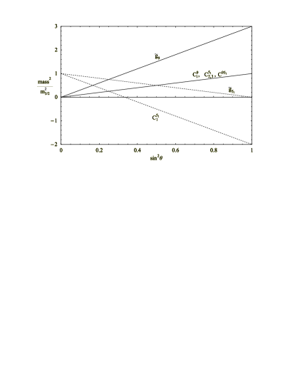
Figure 3: Scalar (C) and gaugino ($\tilde{g}$) squared masses in unit of $m^{2}_{3/2}$ versus $\sin^{2}\theta$ for S/overall modulus ($\Theta_{i}=1/\sqrt{3}$) SUSY breaking when $9$-branes and one set of $5_{1}$-branes are present. The solid lines (with only the scalar fields $C_{i}^{9}$) correspond to the situation where only $9$-brane sectors are present.

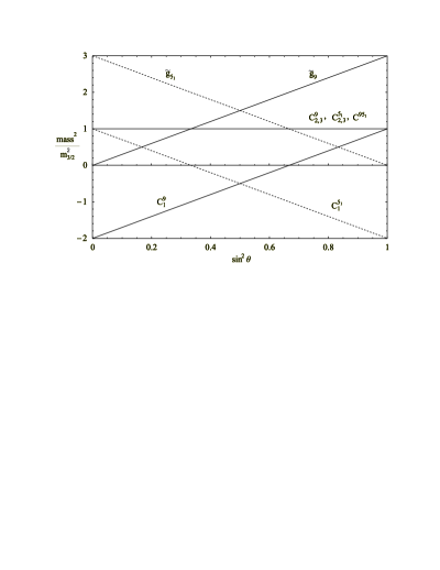
Figure 4: Scalar (C) and gaugino ($\tilde{g}$) squared masses in unit of $m^{2}_{3/2}$ versus $\sin^{2}\theta$ for S/$T_{1}$ ($\Theta_{1}=1$) SUSY breaking when $9$-branes and one set of $5_{1}$-branes are present. The solid lines (with only the scalar fields $C_{i}^{9}$) correspond to the situation where only $9$-brane sectors are present.

2) One immediately observes from (7.12) that the presence of tachyons can be avoided for any choice of the goldstino direction by imposing the condition $\cos^{2}\theta\leq 1/3$. This is shown in Fig.4 with solid lines (only $C_{i}^{9}$ fields are present) for the interesting example $\Theta_{1}=1,\Theta_{2,3}=0$, i.e. $S/T_{1}$ SUSY breaking.

3) The above sum-rule (7.14) implies that scalars heavier than gauginos can exist at the cost of having some of the other three scalars with negative squared mass.

We would like now to study to what extent these conclusions change in the more general case given by (7.7– 7.10) in which there are charged fields both in 9-branes and 5-branes. We insist that this case corresponds to the S-dual of non-perturbative heterotic vacua with a perturbative gauge group (dual to that coming from 9-branes) and a non-perturbative group (dual to that coming from 5-branes).

1) Universality of soft masses

Now, not only scalar masses (7.8) but also gaugino masses (7.7), due to the different values of $f_{\alpha}$ in the different sectors (6.9), are generically non universal. Neither in the dilaton limit, $\sin^{2}\theta=1$, nor in the overall modulus limit, $\Theta_{1,2,3}=\frac{1}{\sqrt{3}}$, universality can be obtained. This can be seen in Fig.3 where the dependence on $\sin^{2}\theta$ of the soft squared masses in orientifold models when 9-branes and one set of $5_{1}$-branes are present is showed. For example, for $\sin^{2}\theta=1$, gauginos in the 9-brane sector, $\tilde{g}_{9}$, have $|M_{9}|=\sqrt{3}m_{3/2}$ whereas gauginos in the $5_{1}$-brane sector, $\tilde{g}_{5_{1}}$, have $M_{5_{1}}=0$. Besides, all scalars have a squared mass equal to $m^{2}_{3/2}$ except $C_{1}^{5_{1}}$ which has a negative squared mass $-2m^{2}_{3/2}$.

One interesting point to emphasize is that there is a value $\sin^{2}\theta=1/4$ which is T-duality self-invariant in this overall modulus situation. Indeed there one has $\frac{F^{S}}{S+S^{*}}=\frac{F^{i}}{T+T^{*}}$. At that point $|M_{9}|=|M_{5_{1}}|=\frac{\sqrt{3}}{2}m_{3/2}$ and all scalars of all sectors have $m=\frac{1}{2}m_{3/2}$.

2) Tachyons

The presence of tachyons cannot be avoided for any choice of the goldstino direction. For example, in the overall modulus limit we see in Fig.3 that there are no tachyons for $\sin^{2}\theta\leq 1/3$. For larger values $C_{1}^{5_{1}}$ becomes tachyonic. However, in Fig.4 we show the direction in which only $S$ and $T_{1}$ contribute to SUSY breaking where either $C_{1}^{9}$ or $C_{1}^{5_{1}}$ (or both) become tachyonic. Let us remark however that this is not necessarily a problem if there are no SM particles in those sectors.

Finally, it is worth noticing that this direction is interesting because the soft terms explicitly show (see Fig.4) the invariance under T-duality which exchanges $S\leftrightarrow T_{1}$. Thus here dilaton dominance and modulus dominance are dual to each other.

3) Gaugino versus scalar masses

Now due to the possibility of having gauginos in different D-brane sectors, 9-brane and $5_{1}$-brane, the sum-rules (7.10) imply that scalars heavier than gauginos can be possible without other scalars becoming tachyonic. We can have $m_{C_{i}^{9}}>|M_{5_{1}}|$ or $m_{C_{i}^{5_{1}}}>|M_{9}|$. For example, in Fig.3 for $\sin^{2}\theta=0$ (modulus-dominated limit) we obtain $m_{C_{1}^{5_{1}}}=m_{3/2}>M_{9}=0$ with $m_{C_{2,3}^{5_{1}}}=m_{C_{i}^{9}}=m_{C^{9{5_{1}}}}=0$ and $M_{5_{1}}=m_{3/2}$.

Comparing these conclusions for two types of branes (9, $5_{1}$) with those summarized above for the perturbative heterotic string (which let us remark again are equivalent to a Type I string with only 9-branes present) one certainly finds plenty of differences. Configurations with three and four types of branes, e.g. (9, $5_{1}$, $5_{2}$) and (9, $5_{1}$, $5_{2}$, $5_{3}$), give rise to similar results. The only difference arises in the configuration with only one set of $5_{i}$-branes, say $5_{1}$-brane. There the existence of universal gaugino masses $M_{5_{1}}$ implies that the sum-rule $m^{2}_{C_{1}^{5_{1}}}+m^{2}_{C_{2}^{5_{1}}}+m^{2}_{C_{3}^{5_{1}}}=M_{5_{1}}^{2}$ (see (7.10)) is fulfilled, without some scalars becoming tachyonic, only if scalars are lighter than gauginos.

8 Anomalous $U(1)$’s, twisted moduli and precocious gauge coupling unification

In the class of Type IIB, $D=4$, orientifold models under discussion there are pseudoanomalous $U(1)$ interactions in the spectrum. Such pseudoanomalous $U(1)$’s are also present in heterotic perturbative vacua although they have different properties than in the orientifold case, as we now discuss.

Let us first recall how are things in the perturbative heterotic case. In that case $D=4$, $N=1$ vacua have at most one anomalous $U(1)_{X}$. The anomaly is canceled by the 4-dimensional version [54, 55, 56] of the Green-Schwarz mechanism [57]. In the latter an important role is played by the imaginary part of the complex heterotic dilaton $S$. Under an anomalous $U(1)_{X}$ gauge transformation with parameter $\theta(x)$ it gets shifted by $c\theta(x)$, c being a constant. Since the Lagrangian contains the couplings $ImS\sum_{a}k_{a}F_{a}\wedge F_{a}$, where the sum runs over all gauge groups in the model, a shift in $ImS$ can in principle cancel mixed $U(1)_{X}$-gauge anomalies. However, for this to be possible the mixed anomalies have to be in the same ratios as the coefficients $k_{a}$ (Kac-Moody levels) of the gauge factors. This is an important constraint which has lead to interesting phenomenological applications [56, 58]. In addition, a Fayet-Iliopoulos (FI) term for the scalar potential associated to the anomalous $U(1)_{X}$ is also generated at one-loop in string theory [54, 59]. This FI term is proportional to ${\rm Tr\,}Q_{X}g/(192\pi^{2})$.

In the case of toroidal $D=4$, $N=1$ Type IIB orientifolds it has been found [35] that the situation is quite different. The main characteristics of anomalous $U(1)$’s in this case are as follows:

i) There are multiple anomalous $U(1)$’s and their mixed anomalies with the rest of the gauge groups are not universal, i.e., they are not in the ratios of the corresponding coupling constants.

ii) There is a generalized Green-Schwarz mechanism at work which cancels all mixed anomalies [35] . In this mechanism the complex dilaton $S$ does not play any role and so happens also with the untwisted moduli fields $T_{i}$. It is the twisted fields $M_{a}$ associated to the fixed points of the underlying orbifold which participate in the cancellation. Furthermore, the required terms appear at the tree (disk) level and not at the one-loop level as in the heterotic case. Specifically, there are two kind of couplings which conspire to get the cancellations. The first of them has the general form:

$$\sum_{k}d^{l}_{k}B_{k}\wedge F_{U(1)_{l}}$$ (8.1)

where $k$ runs over the different twisted sectors of the underlying orbifold (see ref.[35] for details) and $B^{k}$ is the two-form which is the dual to the imaginary part of the twisted fields $M_{a}$. Here l labels the different anomalous $U(1)$’s and $d^{l}_{k}$ are model-dependent constant coefficients. This is a mixing term which connects the anomalous $U(1)$’s with the twisted RR fields associated to the fixed points. The second coupling which participates in the anomaly cancellation is $M_{a}$-dependent piece which appears at the tree-level for the gauge kinetic functions $f_{\alpha}$ corresponding to the different gauge groups $G_{\alpha}$. Thus e.g. for a gauge group coming from p-branes one has in general:

$$f_{\alpha}\ =\ f_{p}\ +\ \sum_{k}s^{\alpha}_{k}M_{k}$$ (8.2)

where $f_{p}$ are the gauge kinetic functions described in section 6 (see e.g. eq.(6.9) ) and $s^{\alpha}_{k}$ are model dependent coefficients. The $M_{k}$ are twisted closed string chiral fields corresponding to the $k$-th twisted sector. The imaginary part of these $M_{k}$ fields are the duals of the $B_{k}$ two-form fields in eq.(8.1).

The generalized Green-Schwarz mechanism works here as follows. An anomalous $U(1)_{l}$ gauge boson mixes with the imaginary part of a twisted $M_{k}$ field (or, equivalently, its dual $B_{k}$ form) as in eq.(8.1). Then the latter propagates and couples to two $G_{\alpha}$ gauge bosons through the second piece in eq.(8.2). This is quite analogous to the mechanism in the perturbative heterotic case, the main difference being that there are several fields (the twisted $M_{a}$ fields) participating in the mechanism. This allows for different mixed anomalies for the different gauge factors. Unfortunately in the present case the details are model dependent since the number of $M_{k}$ fields and the $d^{l}_{k}$, $s^{\alpha}_{k}$ coefficients are indeed model dependent. For some simple examples see ref.[35].

iii) The presence of the mixing term (8.1) and supersymmetry require also the presence of a FI term for each of the anomalous $U(1)$’s [60, 35]:

$$D_{l}\ \sum_{k}d^{l}_{k}ReM_{k}$$ (8.3)

where $D_{l}$ is the auxiliary field for each of the anomalous $U(1)_{l}$ and $ReM_{k}$ are related to the blowing-up modes (twisted moduli) which repair the orbifold singularities. Thus the value of the FI terms is perturbatively undetermined and vanish in the orbifold limit. It has been shown [61] that the one-loop corrections to these FI-terms vanish.

iv) The mass of the anomalous $U(1)$’s depend on the form of the Kahler potential for the twisted fields $M_{k}$. Assuming a Kahler potential of the form $K_{M}=(M_{k}+M_{k}^{*})^{2}$ it is easy to check [61] that all anomalous $U(1)$’s get a mass of order the string scale. If the Kahler potential turns out to have a more complicated form, the mass of the given $U(1)$ would depend on the size of the corresponding FI term and hence could be both heavy or light. Notice that in the first case the anomalous $U(1)$’s would be massive even if the FI terms vanish. Thus in this case the anomalous $U(1)$ would remain like perturbatively exact global symmetries. This could be important in order to insure proton stability in particular string models.

The consequences of the above described FI terms for the dynamics of the models are again very model-dependent since they depend on the twisted sectors of the theories. Nevertheless we would like to point out some other possible phenomenological consequences of the above results.

a) Gauge coupling non-universality and precocious unification

The twisted moduli $M_{k}$ dependent piece in the gauge kinetic functions can have important implications. Notice in particular that this piece is different for different gauge groups, even if all group factor come from the same set of p-branes. Away from the orbifold limit (i.e., $\langle ReM_{k}\rangle\not=0$ ) the gauge couplings will be different and hence there is no universality of gauge couplings. Of course, we already saw in section 3 that if gauge groups come from different types of p-branes there is already no universality of gauge couplings. What we are saying now is that even if all gauge groups come from the same collection of p-branes, the gauge couplings could be different as long as we are close to (but not on top of) the orbifold singularity.

On the other hand this non-universality could be interesting in obtaining gauge coupling unification in low string scale models. For example, in the scheme of ref.[16] with a string scale $M_{I}\approx\sqrt{M_{W}M_{Planck}}$ one has to achieve gauge coupling unification also at that scale which is of order $10^{11}$ GeV. The addition of extra chiral fields in the massless spectrum to achieve precocious gauge coupling unification is a possibility [16]. Here we would like to point out another option which naturally appears in the present context. Consider the renormalization group running of gauge couplings $g_{\alpha}$ from the weak scale to the string scale $M_{I}$:

$${{4\pi}\over{g_{\alpha}(M_{W})}}\ =\ {Ref_{\alpha}}\ +\ {{b_{\alpha}}\over{2\pi}}\log{{M_{I}}\over{M_{W}}}$$ (8.4)

where $f_{\alpha}$ is the gauge kinetic function in eq.(8.2). We know that with the particle content of the MSSM coupling unification works nicely for a unification scale $M_{X}=2\times 10^{16}$ GeV. Now consider a simplified situation with only one relevant $M_{k}$ twisted field. Eq.(8.2) would have the form

$$f_{\alpha}=S\ +\ s_{\alpha}M\ .$$ (8.5)

Thus if we had a model with:

$$s_{\alpha}=\gamma b_{\alpha}\ ;\quad\langle ReM\rangle\ =\ {1\over\gamma}{1\over{2\pi}}\log(M_{X}/M_{I})$$ (8.6)

we would nicely get gauge coupling unification.

It turns out that some odd order compact orientifolds ($Z_{3}$, $Z_{7}$) have the required interesting property that $s_{\alpha}\propto b_{\alpha}$, where in this case $M$ is the sum over all the twisted moduli fields. Let us describe the $D=4$, $N=1$, $Z_{3}$ orientifold [22] as an example. This model contains only 9-branes and has gauge group $U(12)\times SO(8)$ and charged chiral fields transforming as $3(12,8_{v})_{1}$$+3({\overline{66}},1)_{-2}$, where the subindex shows the $U(1)$ charges. The beta functions of the $SU(12)$ and $SO(8)$ groups are respectively $-9$ and $+18$. On the other hand the coefficients $s_{SU(12)}$ and $s_{SO(8)}$ in this model are given by $\cos 2\pi V_{\alpha}$ (see eq.(3.4) in ref.[35]), where $V_{SU(12)}=2/3$ and $V_{SO(8)}=0$. Thus we have $s_{SU(12)}=-1/2$ and $s_{SO(8)}=+1$, indeed proportional to the beta functions. Something analogous does also happen in the $Z_{7}$ orientifold and also if we add Wilson lines to the models.

These are just specific examples and it is not clear to what extent this property could be more general. Nevertheless the orientifold examples show that indeed it is not unreasonable the above scheme for gauge coupling unification for models with low string scales. In principle it should also be applicable to models with $M_{I}=1$ TeV where the problem of precocious gauge unification is more difficult to obtain by other means. Of course, a realistic model with the required properties remains to be built.

b) Corrections to SUSY-breaking soft terms

The results obtained in the previous section for gaugino masses did not take into account the extra piece (8.2) which can appear in the context of orientifold models. Of course, those formula remain valid as long as the twisted $M_{k}$ fields do not participate in the process of SUSY breaking, i.e., $F_{M_{k}}=0$. One important point to realize is that these twisted fields live only close to each singularity, they do not leave in the bulk of the six compact dimensions. Thus they do not participate in the transmission of SUSY breaking from one (hidden) p-brane sector to another (visible) p-brane sector. Thus, unlike what one would have expected, having $F_{M_{k}}\not=0$ in a hidden p-brane sector does not in general gives rise to non-universalities in gaugino masses since the $M_{k}$ fields which couple to differently positioned p-branes are different fields. However, although universality is not affected, the soft mass terms are modified with respect to the results in the previous section because now in general the goldstino field will have a $M_{k}$ component also.

The role of these $M_{k}$ twisted fields in soft terms is somewhat similar to that considered in chapter 8 of ref.[33]. There it was studied the effect of fields contributing to SUSY breaking but not coupling to the visible world. One then has to introduce an extra goldstino angle. This fact was already pointed out in ref.[16].

Let us end this section by emphasizing that the effects discussed here are present in $D=4$, $N=1$ Type IIB orientifold models and need not be present perhaps in more general Type I constructions. In particular, it turns out that in the case of smooth Calabi-Yau compactification of the $D=10$ Type I string, there is again a single anomalous $U(1)$ whose anomaly is canceled by a Green-Schwarz mechanism analogous to the one in perturbative heterotic vacua. In particular, it is the exchange of the complex dilaton field $S$ which cancels the anomaly. On the other hand it seems likely that, whenever we have sets of e.g., 3-branes sitting close to some sort of (not necessarily an orbifold) singularity similar effects will be present.

9 Final comments and outlook

In the present paper we have studied a number of properties of Type IIB, $D=4$, $N=1$ orientifolds which can be phenomenologically relevant. We consider these vacua as interesting laboratories to explore the phenomenological consequences of a D-brane view of the unification of the standard model and gravity. More general vacua which may involve other Type IIA or Type IIB D-brane configurations which go beyond toroidal orbifolds may perhaps be necessary for a final realistic description of the real world, but we hope that some of the generic features found in toroidal orientifolds could still be present in more general situations.

One can conceive more general models which will still be describable in terms of different sets of Dp-branes (one of them containing the SM) sitting either at singularities of the compact space or in the bulk. Chirality of the SM seems to suggest that the Dp-brane set describing the SM should be sitting close to some singularity in compact space, Dp-branes in the bulk give rise generically to vector-like spectra. Those singularities need not be simple orbifold singularities.

A generic vacuum may also contain non-supersymmetric Dp-brane sectors coming e.g. from Dp-branes wrapping on non-supersymmetric cycles of the compact six-dimensional space [62]. If that is the case, lowering the string scale well below the Planck scale may be not just possible but mandatory. Indeed, if we have a vacuum with a $N=1$ p-brane sector containing the SM and other $N=0$ sectors away from it and with a string scale close to $M_{Planck}$, SUSY-breaking terms will appear in the visible $N=1$ SM sector which are not going to be sufficiently suppressed. In this case, setting $M_{I}\leq\sqrt{M_{W}M_{Planck}}$ will be in general required.

The possibility of decreasing the string scale changes also the perspective concerning the generation of the $M_{W}/M_{Planck}$ hierarchy. It was shown in ref.[16] and we have discussed in more detail in section 5 that in Type I $D=4$ vacua there appear factors of the form $\alpha^{2}(M_{c}/M_{I})^{6}$ for this hierarchy. Thus for $M_{c}<<M_{I}$ one can reproduce the required suppression. The choice of value for $M_{I}$ which minimizes fine-tuning (in the sense of requiring not too small ratio, $M_{c}/M_{I}\approx\alpha\approx 10^{-2}$) is the geometric scale $\sqrt{M_{W}M_{Planck}}$. This assumes a scheme in which SUSY breaking is transmitted from a $N=0$ sector to the visible $N=1$ SM sector by fields living in the bulk.

In a Type I scheme in which SUSY breaking is transmitted from a hidden $N=0$ brane sector to a $N=1$ brane sector containing the SM, the natural candidates for this transmission are the dilaton/moduli fields of the model. Specifically, in the context of Type IIB toroidal $D=4$, $N=1$ orientifolds other closed string chiral fields like the twisted moduli live closed to the orbifold singularities, not in the bulk. Thus it seems sensible to parametrize SUSY breaking in the visible $N=1$ sector in terms of dilaton/moduli spurions as we have described in section 7 in the spirit of refs.[33, 34].

Lowering the string scale has its shortcomings. One of them is the question of gauge coupling unification. In a scheme with the string scale of order $M_{X}=2\times 10^{16}$ GeV, gauge coupling unification is nicely achieved. In section 3 we have studied in detail how that happens for different Dp-brane configurations. On the other hand the hierarchy $M_{W}/M_{Planck}$ needs to have its origin in a specifically assumed hierarchy-generating mechanism like gaugino condensation. In schemes with a low string scale (lower than $M_{X}$) one expects the running of SM couplings to stop at the string scale where they are not yet unified. In section 8 we have suggested a possibility to understand this lack of unification at the string scale. If the SM p-branes sit close to a singularity (which anyway seems to be required in order to get chirality) there are tree-level contributions to the gauge couplings which are generically different for each gauge group. If these contributions are proportional to the beta-function of each group they split the couplings in the appropriate way to understand lack of unification. It turns out that there exist specific Type IIB $D=4$, $N=1$ orientifolds in which indeed these contributions to gauge couplings are proportional to the beta functions. This at least shows that this mechanism is a new possibility to understand the question of gauge coupling unification in low string scale models. If this mechanism is indeed at work, it would mean that the branes at which the SM lives sat close to singularity in the compact space.

Another potential problem for low string scale models is nucleon stability. The lower the string scale, the higher the dimension of possible operators one has to worry about. Anyway, dimension=4,5 are a problem in all schemes, including those with $M_{I}=M_{X}$. In all cases there must be extra continuous or discrete (gauge symmetries) suppressing appropriately proton decay. A number of possibilities both for discrete and continuous gauge symmetries ensuring proton stability were studied in ref.[63] . Moreover, Type II string vacua seem to have generically abundant $U(1)$ symmetries, most of them anomalous which could play an important role in ensuring proton stability.

In summary, recent developments in string dualities have changed in many ways our views concerning how to embed the observed physics inside string theory. Surely there will be more surprises waiting for us.

Acknowledgements

We thank C. Burgess, A. Donini, F. Quevedo , R. Rabadan, A. Uranga and G. Violero for discussions.

S. Rigolin acknowledges the European Union for financial support through contract ERBFMBICT972474.

References

-
[1]
For reviews and references, see:
F. Quevedo, hep-ph/9707434; hep-th/9603074;
K. Dienes, hep-th/9602045;
J. Lykken, hep-th/9607144;
G. Aldazabal, hep-th/9507162;
L. E. Ibáñez, hep-th/9505098;
Z. Kakushadze and S.-T. Tye, hep-th/9512155. - [2] For a review, see: J. Polchinski, hep-th/9611050.
- [3] E. Witten, Nucl. Phys. B471 (1996) 135, hep-th/9602070.
- [4] J.D. Lykken, Phys. Rev. D54 (1996) 3693, hep-th/9603133.
- [5] N. Arkani-Hamed, S. Dimopoulos and G. Dvali, hep-ph/9803315.
-
[6]
I. Antoniadis, N. Arkani-Hamed, S. Dimopoulos and G. Dvali,
hep-ph/9804398;
I. Antoniadis, S. Dimopoulos, A. Pomarol and M. Quiros, hep-ph/9810410. - [7] K. Dienes, E. Dudas and T. Gherghetta, hep-ph/9803466; hep-ph/9806292; hep-ph/9807522.
- [8] D. Ghilencea and G.G. Ross, hep-ph/9809217.
- [9] R. Sundrum, hep-ph/9805471; hep-ph/9807348.
- [10] G. Shiu and S.H. Tye, hep-th/9805157.
- [11] C. Bachas, hep-ph/9807415.
- [12] Z. Kakushadze and S.H. Tye, hep-th/9809147.
- [13] K. Benakli, hep-ph/9809582.
-
[14]
K. Benakli and S. Davidson, hep-ph/9810280;
D.H. Lyth, hep-ph/9810320. -
[15]
N. Arkani-Hamed, S. Dimopoulos and G. Dvali, hep-ph/9807344;
P. Argyres, S. Dimopoulos and J. March-Russell, hep-th/9808138;
K. R. Dienes, E. Dudas, T. Gherghetta and A. Riotto, hep-ph/9809406;
N. Arkani-Hamed, S. Dimopoulos and J. March-Russell, hep-th/9809124;
L. Randall and R. Sundrum, hep-th/9810155. - [16] C. Burgess, L.E. Ibáñez and F. Quevedo, hep-ph/9810535.
- [17] Z. Kakushadze, hep-th/9811193.
-
[18]
M. Maggiore and A. Riotto, hep-th/9811089;
G. Giudice, R. Rattazzi and J.D. Wells, hep-ph/9811291;
S. Nussinov and R. Shrock, hep-ph/9811323;
T. Han, J.D. Lykken and R.J. Zhang, hep-ph/9811350;
E.A. Mirabelli, M. Perelstein and M.E. Peskin, hep-ph/9811337;
N. Arkani-Hamed and S. Dimopoulos, hep-ph/9811353;
J. Hewett, hep-ph/9811356;
Z. Berezhiani and G. Dvali, hep-ph/9811378;
K.R. Dienes, E. Dudas and A. Gherghetta, hep-ph/9811428;
N. Arkani-Hamed, S. Dimopoulos and J. March-Russell, hep-ph/9811448;
P. Mathews, S. Raychaudhuri and K. Sridhar, hep-ph/9811501. - [19] L. Dixon, J.A. Harvey, C. Vafa and E. Witten, Nucl. Phys. B261 (1985) 678; B274 1986 285.
-
[20]
L.E. Ibáñez, J. Mas, H.P. Nilles and F. Quevedo,
Nucl. Phys. B301 (1988) 157;
A. Font, L.E. Ibáñez, F. Quevedo and A. Sierra, Nucl. Phys. B331 (1990) 421. - [21] M. Berkooz and R. G. Leigh, Nucl. Phys. B483 (1997) 187, hep-th/9605049.
- [22] C. Angelantonj, M. Bianchi, G. Pradisi, A. Sagnotti and Ya.S. Stanev, Phys. Lett. B385 (1996) 96, hep-th/9606169.
-
[23]
Z. Kakushadze, Nucl. Phys. B512 (1998) 221, hep-th/9704059;
Z. Kakushadze and G. Shiu, Phys. Rev. D56 (1997) 3686, hep-th/9705163;
Z. Kakushadze and G. Shiu, Nucl. Phys. B520 1998 75, hep-th/9706051. - [24] G. Zwart, Nucl. Phys. B526 (1998) 378, hep-th/9708040.
- [25] D. O’Driscoll, hep-th/9801114.
- [26] L.E. Ibáñez, hep-th/9802103.
- [27] G. Aldazabal, A. Font, L.E. Ibáñez and G. Violero, FTUAM-98/4, hep-th/9804026.
- [28] Z. Kakushadze, hep-th/9804110; hep-th/9806044.
- [29] J. Lykken, E. Poppitz and S. Trivedi, hep-th/9806080.
- [30] For a recent review, see: A. Brignole, L.E. Ibáñez and C. Muñoz, in the book ‘Perspectives on Supersymmetry’, Ed. G. Kane, (World Scientific, 1998) p. 125; hep-ph/9707209.
- [31] L.E. Ibáñez and D. Lüst, Nucl. Phys. B382 (1992) 305.
- [32] V.S. Kaplunovsky and J. Louis, Phys. Lett. B306 (1993) 269.
- [33] A. Brignole, L.E. Ibáñez and C. Muñoz, Nucl. Phys. B422 (1994) 125 [Erratum: B436 (1995) 747].
- [34] A. Brignole, L.E. Ibáñez, C. Muñoz and C. Scheich, Z. Phys. C74 (1997) 157.
- [35] L. E. Ibáñez, R. Rabadán and A. Uranga, hep-th/9808139 .
- [36] L.E. Ibáñez, hep-ph/9804236.
- [37] A. Sagnotti, in Cargese 87, ‘Strings on Orbifolds’, Ed. G. Mack et al. (Pergamon Press, 1988) p. 521.
-
[38]
P. Horava, Nucl. Phys. B327 (1989) 461; Phys. Lett. B231 (1989) 251;
J. Dai, R. Leigh and J. Polchinski, Mod.Phys.Lett. A4 (1989) 2073;
R. Leigh, Mod.Phys.Lett. A4 (1989) 2767. -
[39]
G. Pradisi and A. Sagnotti, Phys. Lett. B216 (1989) 59;
M. Bianchi and A. Sagnotti, Phys. Lett. B247 (1990) 517. - [40] E. Gimon and J. Polchinski, Phys.Rev. D54 (1996) 1667, hep-th/9601038.
- [41] A. Dabholkar and J. Park, Nucl. Phys. B472 (1996) 207, hep-th/9602030.
- [42] E. Gimon and C. Johnson, Nucl. Phys. B477 (1996) 715, hep-th/9604129.
- [43] For an introduction to orientifolds see, e.g.: A. Dabholkar, hep-th/9804208.
- [44] J. Polchinski and E. Witten, Nucl. Phys. B460 (1996) 525 , hep-th/9510169.
- [45] T. Taylor and G. Veneziano, Phys. Lett. B212 (1988) 147.
- [46] P. Horava and E. Witten, Nucl. Phys. B460 (1996) 506, hep-th/9510209; B475 (1996) 94, hep-th/9603142.
-
[47]
T. Banks and M. Dine, Nucl. Phys. B479
(1996) 173, hep-th/9605136;
K. Choi, Phys. Rev. D56 (1997) 6588, hep-th/9706171;
H.P. Nilles and S. Stieberger, Nucl. Phys. B499 (1997) 3, hep-th/9702110. - [48] H.P. Nilles, M. Olechowski and M. Yamaguchi, Phys. Lett. B415 (1997) 24, hep-th/9707143.
- [49] A. Lukas, B.A.Ovrut and D. Waldram, Nucl. Phys. B532 (1998) 43, hep-th/9710208.
- [50] S.K. Soni and H.A. Weldon, Phys. Lett. B126 (1983) 215.
- [51] K. Choi, H.B. Kim and C. Muñoz, Phys. Rev. D57 (1998) 7521, hep-th/9711158.
- [52] A. Lukas, B.A. Ovrut and D. Waldram, Phys. Rev. D57 (1998) 7529, hep-th/971119.
- [53] B. de Carlos, J.A. Casas and C. Muñoz, Phys. Lett. B299 (1993) 234.
- [54] M. Dine, N. Seiberg and E. Witten, Nucl. Phys. B289 (1987) 585.
- [55] J. Casas, E. Katehou and C. Muñoz, Nucl. Phys. B317 (1989) 171.
- [56] L.E. Ibáñez, Phys. Lett. B303 (1993) 55.
- [57] M. Green and J. Schwarz, Phys. Lett. B149 (1984) 117.
- [58] L.E. Ibáñez and G.G. Ross, Phys. Lett. B332 (1994) 100; for a review and references, see: P. Ramond, hep-ph/9604251.
-
[59]
J. Atick, L. Dixon and A. Sen, Nucl. Phys. B292 (1987) 109;
M. Dine, I. Ichinoise and N. Seiberg, Nucl. Phys. B293 (1987) 253. - [60] M. Douglas and G. Moore, hep-th/9603167.
- [61] E. Poppitz, hep-th/9810010.
- [62] A. Sen, hep-th/9812031.
- [63] L.E. Ibáñez and G.G. Ross, Nucl. Phys. B368 (1992) 3.