Model-Independent Analysis of $B\to\pi K$ Decays and Bounds on the Weak Phase $\gamma$

Abstract:

A general parametrization of the amplitudes for the rare two-body decays $B\to\pi K$ is introduced, which makes maximal use of theoretical constraints arising from flavour symmetries of the strong interactions and the structure of the low-energy effective weak Hamiltonian. With the help of this parametrization, a model-independent analysis of the branching ratios and direct CP asymmetries in the various $B\to\pi K$ decay modes is performed, and the impact of hadronic uncertainties on bounds on the weak phase $\gamma=\mbox{arg}(V_{ub}^{*})$ is investigated.

1 Introduction

The CLEO Collaboration has recently reported the observation of some rare two-body decays of the type $B\to\pi K$, as well as interesting upper bounds for the decays $B\to\pi\pi$ and $B\to K\bar{K}$ [1]. In particular, they find the CP-averaged branching ratios

$$\frac{1}{2}\Big{[}\mbox{Br}(B^{0}\to\pi^{-}K^{+})+\mbox{Br}(\bar{B}^{0}\to\pi^{+}K^{-})\Big{]} = (1.4\pm 0.3\pm 0.1)\times 10^{-5}\,,$$

$$\frac{1}{2}\Big{[}\mbox{Br}(B^{+}\to\pi^{+}K^{0})+\mbox{Br}(B^{-}\to\pi^{-}\bar{K}^{0})\Big{]} = (1.4\pm 0.5\pm 0.2)\times 10^{-5}\,,$$

$$\frac{1}{2}\Big{[}\mbox{Br}(B^{+}\to\pi^{0}K^{+})+\mbox{Br}(B^{-}\to\pi^{0}K^{-})\Big{]} = (1.5\pm 0.4\pm 0.3)\times 10^{-5}\,.$$ (1)

This observation caused a lot of excitement, because these decays offer interesting insights into the relative strength of various contributions to the decay amplitudes, whose interference can lead to CP asymmetries in the decay rates. It indeed appears that there may be potentially large interference effects, depending on the magnitude of some strong interaction phases (see, e.g., [2]). Thus, although at present only measurements of CP-averaged branching ratios have been reported, the prospects are good for observing direct CP violation in some of the $B\to\pi K$ or $B\to K\bar{K}$ decay modes in the near future.

It is fascinating that some information on CP-violating parameters can be extracted even without observing a single CP asymmetry, from measurements of CP-averaged branching ratios alone. This information concerns the angle $\gamma$ of the so-called unitarity triangle, defined as $\gamma=\mbox{arg}[(V_{ub}^{*}V_{ud})/(V_{cb}^{*}V_{cd})]$. With the standard phase conventions for the Cabibbo–Kobayashi–Maskawa (CKM) matrix, $\gamma=\mbox{arg}(V_{ub}^{*})$ to excellent accuracy. There have been proposals for deriving bounds on $\gamma$ from measurements of the ratios

$$R = \frac{\tau(B^{+})}{\tau(B^{0})}\,\frac{\mbox{Br}(B^{0}\to\pi^{-}K^{+})+\mbox{Br}(\bar{B}^{0}\to\pi^{+}K^{-})}{\mbox{Br}(B^{+}\to\pi^{+}K^{0})+\mbox{Br}(B^{-}\to\pi^{-}\bar{K}^{0})}\,,$$

$$R_{*} = \frac{\mbox{Br}(B^{+}\to\pi^{+}K^{0})+\mbox{Br}(B^{-}\to\pi^{-}\bar{K}^{0})}{2[\mbox{Br}(B^{+}\to\pi^{0}K^{+})+\mbox{Br}(B^{-}\to\pi^{0}K^{-})]}\,,$$ (2)

whose current experimental values are $R=1.07\pm 0.45$ (we use $\tau(B^{+})/\tau(B^{0})=1.07\pm 0.03$) and $R_{*}=0.47\pm 0.24$. The Fleischer–Mannel bound $R\geq\sin^{2}\!\gamma$ [3] excludes values around $|\gamma|=90^{\circ}$ provided that $R<1$. However, this bound is subject to theoretical uncertainties arising from electroweak penguin contributions and strong rescattering effects, which are difficult to quantify [4]–[9]. The bound

$$1-\sqrt{R_{*}}\leq\bar{\varepsilon}_{3/2}\,|\delta_{\rm EW}-\cos\gamma|+O(\bar{\varepsilon}_{3/2}^{2})$$ (3)

derived by Rosner and the present author [10], where $\delta_{\rm EW}=0.64\pm 0.15$ accounts for electroweak penguin contributions, is less affected by such uncertainties; however, it relies on an expansion in the small parameter

$$\bar{\varepsilon}_{3/2}=\sqrt{2}\,R_{\rm SU(3)}\tan\theta_{C}\left[\frac{\mbox{Br}(B^{+}\to\pi^{+}\pi^{0})+\mbox{Br}(B^{-}\to\pi^{-}\pi^{0})}{\mbox{Br}(B^{+}\to\pi^{+}K^{0})+\mbox{Br}(B^{-}\to\pi^{-}\bar{K}^{0})}\right]^{1/2}\,,$$ (4)

whose value has been estimated to be $\bar{\varepsilon}_{3/2}=0.24\pm 0.06$. Here $\theta_{C}$ is the Cabibbo angle, and the factor $R_{\rm SU(3)}\simeq f_{K}/f_{\pi}$ accounts for SU(3)-breaking corrections. Assuming the smallness of certain rescattering effects, higher-order terms in the expansion in $\bar{\varepsilon}_{3/2}$ can be shown to strengthen the bound (3) provided that the value of $R_{*}$ is not much larger than indicated by current data, i.e., if $R_{*}<(1-\bar{\varepsilon}_{3/2}/\sqrt{2})^{2}\approx 0.7$ [10].

Our main goal in the present work is to address the question to what extent these bounds can be affected by hadronic uncertainties such as final-state rescattering effects, and whether the theoretical assumptions underlying them are justified. To this end, we perform a general analysis of the various $B\to\pi K$ decay modes, pointing out where theoretical information from isopsin and SU(3) flavour symmetries can be used to eliminate hadronic uncertainties. Our approach will be to vary parameters not constrained by theory (strong-interaction phases, in particular) within conservative ranges so as to obtain a model-independent description of the decay amplitudes. An analysis pursuing a similar goal has recently been presented by Buras and Fleischer [11]. Where appropriate, we will point out the relations of our work with theirs and provide a translation of notations. We stress, however, that although we take a similar starting point, some of our conclusions will be rather different from the ones reached in their work.

In Section 2, we present a general parametrization of the various isospin amplitudes relevant to $B\to\pi K$ decays and discuss theoretical constraints resulting from flavour symmetries of the strong interactions and the structure of the low-energy effective weak Hamiltonian. We summarize model-independent results derived recently for the electroweak penguin contributions to the isovector part of the effective Hamiltonian [6, 9] and point out constraints on certain rescattering contributions resulting from $B\to K\bar{K}$ decays [7, 9, 12, 13]. The main results of this analysis are presented in Section 2.6, which contains numerical predictions for the various parameters entering our parametrization of the decay amplitudes. The remainder of the paper deals with phenomenological applications of these results. In Section 3, we discuss corrections to the Fleischer–Mannel bound resulting from final-state rescattering and electroweak penguin contributions. In Section 4, we show how to include rescattering effects to the bound (3) at higher orders in the expansion in $\bar{\varepsilon}_{3/2}$. Detailed predictions for the direct CP asymmetries in the various $B\to\pi K$ decay modes are presented in Section 5, where we also present a prediction for the CP-averaged $B^{0}\to\pi^{0}K^{0}$ branching ratio, for which at present only an upper limit exists. In Section 6, we discuss how the weak phase $\gamma$, along with a strong-interaction phase difference $\phi$, can be determined from measurements of the ratio $R_{*}$ and of the direct CP asymmetries in the decays $B^{\pm}\to\pi^{0}K^{\pm}$ and $B^{\pm}\to\pi^{\pm}K^{0}$ (here $K^{0}$ means $K^{0}$ or $\bar{K}^{0}$, as appropriate). This generalizes a method proposed in [14] to include rescattering corrections to the $B^{\pm}\to\pi^{\pm}K^{0}$ decay amplitudes. Section 7 contains a summary of our result and the conclusions.

2 Isospin decomposition

2.1 Preliminaries

The effective weak Hamiltonian relevant to the decays $B\to\pi K$ is [15]

$${\mathcal{H}}=\frac{G_{F}}{\sqrt{2}}\,\bigg{\{}\sum_{i=1,2}C_{i}\Big{(}\lambda_{u}\,Q_{i}^{u}+\lambda_{c}\,Q_{i}^{c}\Big{)}-\lambda_{t}\sum_{i=3}^{10}C_{i}\,Q_{i}\bigg{\}}+\mbox{h.c.}\,,$$ (5)

where $\lambda_{q}=V_{qb}^{*}V_{qs}$ are products of CKM matrix elements, $C_{i}$ are Wilson coefficients, and $Q_{i}$ are local four-quark operators. Relevant to our discussion are the isospin quantum numbers of these operators. The current–current operators $Q_{1,2}^{u}\sim\bar{b}s\bar{u}u$ have components with $\Delta I=0$ and $\Delta I=1$; the current–current operators $Q_{1,2}^{c}\sim\bar{b}s\bar{c}c$ and the QCD penguin operators $Q_{3,\dots,6}\sim\bar{b}s\sum\bar{q}q$ have $\Delta I=0$; the electroweak penguin operators $Q_{7,\dots,10}\sim\bar{b}s\sum e_{q}\bar{q}q$, where $e_{q}$ are the electric charges of the quarks, have $\Delta I=0$ and $\Delta I=1$. Since the initial $B$ meson has $I=\frac{1}{2}$ and the final states $(\pi K)$ can be decomposed into components with $I=\frac{1}{2}$ and $I=\frac{3}{2}$, the physical $B\to\pi K$ decay amplitudes can be described in terms of three isospin amplitudes. They are called $B_{1/2}$, $A_{1/2}$, and $A_{3/2}$ referring, respectively, to $\Delta I=0$ with $I_{\pi K}=\frac{1}{2}$, $\Delta I=1$ with $I_{\pi K}=\frac{1}{2}$, and $\Delta I=1$ with $I_{\pi K}=\frac{3}{2}$ [6, 16, 17]. The resulting expressions for the decay amplitudes are

$${\mathcal{A}}(B^{+}\to\pi^{+}K^{0}) = B_{1/2}+A_{1/2}+A_{3/2}\,,$$

$$-\sqrt{2}\,{\mathcal{A}}(B^{+}\to\pi^{0}K^{+}) = B_{1/2}+A_{1/2}-2A_{3/2}\,,$$

$$-{\mathcal{A}}(B^{0}\to\pi^{-}K^{+}) = B_{1/2}-A_{1/2}-A_{3/2}\,,$$

$$\sqrt{2}\,{\mathcal{A}}(B^{0}\to\pi^{0}K^{0}) = B_{1/2}-A_{1/2}+2A_{3/2}\,.$$ (6)

From the isospin decomposition of the effective Hamiltonian it is obvious which operator matrix elements and weak phases enter the various isospin amplitudes. Experimental data as well as theoretical expectations indicate that the amplitude $B_{1/2}$, which includes the contributions of the QCD penguin operators, is significantly larger than the amplitudes $A_{1/2}$ and $A_{3/2}$ [2, 6]. Yet, the fact that $A_{1/2}$ and $A_{3/2}$ are different from zero is responsible for the deviations of the ratios $R$ and $R_{*}$ in (2) from 1.

Because of the unitarity relation $\lambda_{u}+\lambda_{c}+\lambda_{t}=0$ there are two independent CKM parameters entering the decay amplitudes, which we choose to be $-\lambda_{c}=e^{i\pi}|\lambda_{c}|$ and $\lambda_{u}=e^{i\gamma}|\lambda_{u}|$. Each of the three isospin amplitudes receives contributions proportional to both weak phases. In total, there are thus five independent strong-interaction phase differences (an overall phase is irrelevant) and six independent real amplitudes, leaving as many as eleven hadronic parameters. Even perfect measurements of the eight branching ratios for the various $B\to\pi K$ decay modes and their CP conjugates would not suffice to determine these parameters. Facing this problem, previous authors have often relied on some theoretical prejudice about the relative importance of various parameters. For instance, in the invariant SU(3)-amplitude approach based on flavour-flow topologies [18, 19], the isospin amplitudes are expressed as linear combinations of a QCD penguin amplitude $P$, a tree amplitude $T$, a colour-suppressed tree amplitude $C$, an annihilation amplitide $A$, an electroweak penguin amplitude $P_{\rm EW}$, and a colour-suppressed electroweak penguin amplitude $P_{\rm EW}^{C}$, which are expected to obey the following hierarchy: $|P|\gg|T|\sim|P_{\rm EW}|\gg|C|\sim|P_{\rm EW}^{C}|>|A|$. These naive expectations could be upset, however, if strong final-state rescattering effects would turn out to be important [5]–[8], a possibility which at present is still under debate. Whereas the colour-transparency argument [20] suggests that final-state interactions are small in $B$ decays into a pair of light mesons, the opposite behaviour is exhibited in a model based on Regge phenomenology [21]. For comparison, we note that in the decays $B\to D^{(*)}h$, with $h=\pi$ or $\rho$, the final-state phase differences between the $I=\frac{1}{2}$ and $I=\frac{3}{2}$ isospin amplitudes are found to be smaller than $30^{\circ}$–$50^{\circ}$ [22].

Here we follow a different strategy, making maximal use of theoretical constraints derived using flavour symmetries and the knowledge of the effective weak Hamiltonian in the Standard Model. These constraints help simplifying the isospin amplitude $A_{3/2}$, for which the two contributions with different weak phases turn out to have the same strong-interaction phase (to an excellent approximation) and magnitudes that can be determined without encountering large hadronic uncertainties [10]. Theoretical uncertainties enter only at the level of SU(3)-breaking corrections, which can be accounted for using the generalized factorization approximation [22]. Effectively, these simplifications remove three parameters (one phase and two magnitudes) from the list of unknown hadronic quantities. There is at present no other clean theoretical information about the remaining parameters, although some constraints can be derived using measurements of the branching ratios for the decays $B^{\pm}\to K^{\pm}\bar{K}^{0}$ and invoking SU(3) symmetry [7, 9, 12, 13]. Nevertheless, interesting insights can be gained by fully exploiting the available information on $A_{3/2}$.

Before discussing this in more detail, it is instructive to introduce certain linear combinations of the isospin amplitudes, which we define as

$$B_{1/2}+A_{1/2}+A_{3/2} = P+A-\frac{1}{3}P_{\rm EW}^{C}\,,$$

$$-3A_{3/2} = T+C+P_{\rm EW}+P_{\rm EW}^{C}\,,$$

$$-2(A_{1/2}+A_{3/2}) = T-A+P_{\rm EW}^{C}\,.$$ (7)

In the latter two relations, the amplitudes $T$, $C$ and $A$ carry the weak phase $e^{i\gamma}$, whereas the electroweak penguin amplitudes $P_{\rm EW}$ and $P_{\rm EW}^{C}$ carry the weak phase $e^{i\pi}$. Decomposing the QCD penguin amplitude as $P=\sum_{q}\lambda_{q}P_{q}$, and similarly writing $A=\lambda_{u}A_{u}$ and $P_{\rm EW}^{C}=\lambda_{t}P_{{\rm EW},t}^{C}$, we rewrite the first relation in the form

$$B_{1/2}+A_{1/2}+A_{3/2} = -\lambda_{c}(P_{t}-P_{c}-\textstyle\frac{1}{3}P_{{\rm EW},t}^{C})+\lambda_{u}(A_{u}-P_{t}+P_{u})$$ (8)

$$\equiv |P|\,e^{i\phi_{P}}\Big{(}e^{i\pi}+\varepsilon_{a}\,e^{i\gamma}e^{i\eta}\Big{)}\,.$$

By definition, the term $|P|\,e^{i\phi_{P}}e^{i\pi}$ contains all contributions to the $B^{+}\to\pi^{+}K^{0}$ decay amplitude not proportional to the weak phase $e^{i\gamma}$. We will return to a discussion of the remaining terms below. It is convenient to adopt a parametrization of the other two amplitude combinations in (7) in units of $|P|$, so that this parameter cancels in predictions for ratios of branching ratios. We define

$$\frac{-3A_{3/2}}{|P|} = \varepsilon_{3/2}\,e^{i\phi_{3/2}}(e^{i\gamma}-q\,e^{i\omega})\,,$$

$$\frac{-2(A_{1/2}+A_{3/2})}{|P|} = \varepsilon_{T}\,e^{i\phi_{T}}(e^{i\gamma}-q_{C}\,e^{i\omega_{C}})\,,$$ (9)

where the terms with $q$ and $q_{C}$ arise from electroweak penguin contributions. In the above relations, the parameters $\eta$, $\phi_{3/2}$, $\phi_{T}$, $\omega$, and $\omega_{C}$ are strong-interaction phases. For the benefit of the reader, it may be convenient to relate our definitions in (8) and (9) with those adopted by Buras and Fleischer [11]. The identificantions are: $|P|\,e^{i\phi_{P}}\leftrightarrow\lambda_{c}|P_{tc}|\,e^{i\delta_{tc}}$, $\varepsilon_{a}\,e^{i\eta}\leftrightarrow-\rho\,e^{i\theta}$, $\phi_{3/2}\leftrightarrow\delta_{T+C}$, and $\phi_{T}\leftrightarrow\delta_{T}$. The notations for the electroweak penguin contributions conincide. Moreover, if we define

$$\bar{\varepsilon}_{3/2}\equiv\frac{\varepsilon_{3/2}}{\sqrt{1-2\varepsilon_{a}\cos\eta\cos\gamma+\varepsilon_{a}^{2}}}\,,$$ (10)

then $\bar{\varepsilon}_{3/2}\leftrightarrow r_{\rm c}$ and $\varepsilon_{T}/\varepsilon_{3/2}\leftrightarrow r/r_{\rm c}$. With this definition, the parameter $\bar{\varepsilon}_{3/2}$ is precisely the quantity that can be determined experimentally using the relation (4).

2.2 Isovector part of the effective weak Hamiltonian

The two amplitude combinations in (9) involve isospin amplitudes defined in terms of the strong-interaction matrix elements of the $\Delta I=1$ part of the effective weak Hamiltonian. This part contains current–current as well as electroweak penguin operators. A trivial but relevant observation is that the electroweak penguin operators $Q_{9}$ and $Q_{10}$, whose Wilson coefficients are enhanced by the large mass of the top quark, are Fierz-equivalent to the current–current operators $Q_{1}$ and $Q_{2}$ [6, 9, 23]. As a result, the $\Delta I=1$ part of the effective weak Hamiltonian for $B\to\pi K$ decays can be written as

$${\mathcal{H}}_{\Delta I=1}=\frac{G_{F}}{\sqrt{2}}\left\{\left(\lambda_{u}C_{1}-\frac{3}{2}\lambda_{t}C_{9}\right)\bar{Q}_{1}+\left(\lambda_{u}C_{2}-\frac{3}{2}\lambda_{t}C_{10}\right)\bar{Q}_{2}+\dots\right\}+\mbox{h.c.}\,,$$ (11)

where $\bar{Q}_{i}=\frac{1}{2}(Q_{i}^{u}-Q_{i}^{d})$ are isovector combinations of four-quark operators. The dots represent the contributions from the electroweak penguin operators $Q_{7}$ and $Q_{8}$, which have a different Dirac structure. In the Standard Model, the Wilson coefficients of these operators are so small that their contributions can be safely neglected. It is important in this context that for heavy mesons the matrix elements of four-quark operators with Dirac structure $(V-A)\otimes(V+A)$ are not enhanced with respect to those of operators with the usual $(V-A)\otimes(V-A)$ structure. To an excellent approximation, the net effect of electroweak penguin contributions to the $\Delta I=1$ isospin amplitudes in $B\to\pi K$ decays thus consists of the replacements of the Wilson coefficients $C_{1}$ and $C_{2}$ of the current–current operators with the combinations shown in (11). Introducing the linear combinations $C_{\pm}=(C_{2}\pm C_{1})$ and $\bar{Q}_{\pm}=\frac{1}{2}(\bar{Q}_{2}\pm\bar{Q}_{1})$, which have the advantage of being renormalized multiplicatively, we obtain

$${\mathcal{H}}_{\Delta I=1}\simeq\frac{G_{F}}{\sqrt{2}}|V_{ub}^{*}V_{us}|\left\{C_{+}(e^{i\gamma}-\delta_{+})\,\bar{Q}_{+}+C_{-}(e^{i\gamma}-\delta_{-})\,\bar{Q}_{-}\right\}+\mbox{h.c.}\,,$$ (12)

where

$$\delta_{\pm}=-\frac{3\cot\theta_{C}}{2\,|V_{ub}/V_{cb}|}\,\frac{C_{10}\pm C_{9}}{C_{2}\pm C_{1}}\,.$$ (13)

We have used $\lambda_{u}/\lambda_{t}\simeq-\lambda_{u}/\lambda_{c}\simeq-\tan\theta_{C}\,|V_{ub}/V_{cb}|\,e^{i\gamma}$, with the ratio $|V_{ub}/V_{cb}|=0.089\pm 0.015$ determined from semileptonic $B$ decays [24].

From the fact that the products $C_{\pm}\,\bar{Q}_{\pm}$ are renormalization-group invariant, it follows that the quantities $\delta_{\pm}$ themselves must be scheme- and scale-independent (in a certain approximation). Indeed, the ratios of Wilson coefficients entering in (13) are, to a good approximation, independent of the choice of the renormalization scale. Taking the values $C_{1}=-0.308$, $C_{2}=1.144$, $C_{9}=-1.280\alpha$ and $C_{10}=0.328\alpha$, which correspond to the leading-order coefficients at the scale $\mu=m_{b}$ [15], we find $(C_{10}+C_{9})/(C_{2}+C_{1})\approx-1.14\alpha$ and $(C_{10}-C_{9})/(C_{2}-C_{1})\approx 1.11\alpha$, implying that $\delta_{-}\approx-\delta_{+}$ to a good approximation. The statement of the approximate renormalization-group invariance of the ratios $\delta_{\pm}$ can be made more precise by noting that the large values of the Wilson coefficients $C_{9}$ and $C_{10}$ at the scale $\mu=m_{b}$ predominantly result from large matching contributions to the coefficient $C_{9}(m_{W})$ arising from box and $Z$-penguin diagrams, whereas the $O(\alpha)$ contributions to the anomalous dimension matrix governing the mixing of the local operators $Q_{i}$ lead to very small effects. If these are neglected, then to next-to-leading order in the QCD evolution the coefficients $(C_{10}\pm C_{9})$ are renormalized multiplicatively and in precisely the same way as the coefficients $(C_{2}\pm C_{1})$. We have derived this result using the explicit expressions for the anomalous dimension matrices compiled in [15]. Hence, in this approximation the ratios of coefficients entering the quantities $\delta_{\pm}$ are renormalization-scale independent and can be evaluated at the scale $m_{W}$, so that

$$\frac{C_{10}\pm C_{9}}{C_{2}\pm C_{1}}\simeq\pm C_{9}(m_{W})=\mp\frac{\alpha}{12\pi}\,\frac{x_{t}}{\sin^{2}\!\theta_{W}}\left(1+\frac{3\ln x_{t}}{x_{t}-1}\right)+\dots\approx\mp 1.18\alpha\,,$$ (14)

where $\theta_{W}$ is the Weinberg angle, and $x_{t}=(m_{t}/m_{W})^{2}$. This result agrees with an equivalent expression derived by Fleischer [23]. The dots in (14) represent renormalization-scheme dependent terms, which are not enhanced by the factor $1/\sin^{2}\!\theta_{W}$. These terms are numerically very small and of the same order as the coefficients $C_{7}$ and $C_{8}$, whose values have been neglected in our derivation. The leading terms given above are precisely the ones that must be kept to get a consistent, renormalization-group invariant result. We thus obtain

$$\delta_{+}=-\delta_{-}=\frac{\alpha}{8\pi}\,\frac{\cot\theta_{C}}{|V_{ub}/V_{cb}|}\,\frac{x_{t}}{\sin^{2}\!\theta_{W}}\left(1+\frac{3\ln x_{t}}{x_{t}-1}\right)=0.68\pm 0.11\,,$$ (15)

where we have taken $\alpha=1/129$ for the electromagnetic coupling renormalized at the scale $m_{b}$, and $m_{t}=\overline{m}_{t}(m_{t})=170$ GeV for the running top-quark mass in the $\overline{{\rm MS}}$ renormalization scheme. Assuming that there are no large $O(\alpha_{s})$ corrections with this choice, the main uncertainty in the estimate of $\delta_{+}$ in the Standard Model results from the present error on $|V_{ub}|$, which is likely to be reduced in the near future.

We stress that the sensitivity of the $B\to\pi K$ decay amplitudes to the value of $\delta_{+}$ provides a window to New Physics, which could alter the value of this parameter significantly. A generic example are extensions of the Standard Model with new charged Higgs bosons such as supersymmetry, for which there are additional matching contributions to $C_{9}(m_{W})$. We will come back to this point in Section 4.

2.3 Structure of the isospin amplitude $A_{3/2}$

$U$-spin invariance of the strong interactions, which is a subgroup of flavour SU(3) symmetry corresponding to transformations exchanging $d$ and $s$ quarks, implies that the isospin amplitude $A_{3/2}$ receives a contribution only from the operator $\bar{Q}_{+}$ in (12), but not from $\bar{Q}_{-}$ [10]. In order to investigate the corrections to this limit, we parametrize the matrix elements of the local operators $C_{\pm}\bar{Q}_{\pm}$ between a $B$ meson and the $(\pi K)$ isospin state with $I=\frac{3}{2}$ by hadronic parameters $K_{3/2}^{\pm}\,e^{i\phi_{3/2}^{\pm}}$, so that

$$-3A_{3/2} = K_{3/2}^{+}\,e^{i\phi_{3/2}^{+}}(e^{i\gamma}-\delta_{+})+K_{3/2}^{-}\,e^{i\phi_{3/2}^{-}}(e^{i\gamma}+\delta_{+})$$ (16)

$$\equiv \Big{(}K_{3/2}^{+}\,e^{i\phi_{3/2}^{+}}+K_{3/2}^{-}\,e^{i\phi_{3/2}^{-}}\Big{)}(e^{i\gamma}-q\,e^{i\omega})\,.$$

In the SU(3) limit $K_{3/2}^{-}=0$, and hence SU(3)-breaking corrections can be parametrized by the quantity

$$\kappa\,e^{i\Delta\varphi_{3/2}}\equiv\frac{2K_{3/2}^{-}\,e^{i\phi_{3/2}^{-}}}{K_{3/2}^{+}\,e^{i\phi_{3/2}^{+}}+K_{3/2}^{-}\,e^{i\phi_{3/2}^{-}}}=2\left[\frac{K_{3/2}^{+}}{K_{3/2}^{-}}\,e^{i(\phi_{3/2}^{+}-\phi_{3/2}^{-})}+1\right]^{-1}\,,$$ (17)

in terms of which

$$q\,e^{i\omega}=\left(1-\kappa\,e^{i\Delta\varphi_{3/2}}\right)\delta_{+}\,.$$ (18)

This relation generalizes an approximate result derived in [10].

The magnitude of the SU(3)-breaking effects can be estimated by using the generalized factorization hypothesis to calculate the matrix elements of the current–current operators [22]. This gives

$$\kappa\simeq 2\left[\frac{a_{1}+a_{2}}{a_{1}-a_{2}}\,\frac{A_{K}+A_{\pi}}{A_{K}-A_{\pi}}+1\right]^{-1}=(6\pm 6)\%\,,\qquad\Delta\varphi_{3/2}\simeq 0\,,$$ (19)

where $A_{K}=f_{K}(m_{B}^{2}-m_{\pi}^{2})F_{0}^{B\to\pi}(m_{K}^{2})$ and $A_{\pi}=f_{\pi}(m_{B}^{2}-m_{K}^{2})F_{0}^{B\to K}(m_{\pi}^{2})$ are combinations of hadronic matrix elements, and $a_{1}$ and $a_{2}$ are phenomenological parameters defined such that they contain the leading corrections to naive factorization. For a numerical estimate we take $a_{2}/a_{1}=0.21\pm 0.05$ as determined from a global analysis of nonleptonic two-body decays of $B$ mesons [22], and $A_{\pi}/A_{K}=0.9\pm 0.1$, which is consistent with form factor models (see, e.g., [25]–[27]) as well as the most recent predictions obtained using light-cone QCD sum rules [28]. Despite the fact that nonfactorizable corrections are not fully controlled theoretically, the estimate (19) suggests that the SU(3)-breaking corrections in (18) are small. More importantly, such effects cannot induce a sizable strong-interaction phase $\omega$. Since $\bar{Q}_{+}$ and $\bar{Q}_{-}$ are local operators whose matrix elements are taken between the same isospin eigenstates, it is very unlikely that the strong-interaction phases $\phi_{3/2}^{+}$ and $\phi_{3/2}^{-}$ could differ by a large amount. If we assume that these phases differ by at most $20^{\circ}$, and that the magnitude of $\kappa$ is as large as 12% (corresponding to twice the central value obtained using factorization), we find that $|\omega|<2.7^{\circ}$. Even for a phase difference $\Delta\varphi_{3/2}\simeq|\phi_{3/2}^{+}-\phi_{3/2}^{-}|=90^{\circ}$, which seems totally unrealistic, the phase $|\omega|$ would not exceed $7^{\circ}$. It is therefore a safe approximation to work with the real value [10]

$$\delta_{\rm EW}\equiv(1-\kappa)\,\delta_{+}=0.64\pm 0.15\,,$$ (20)

where to be conservative we have added linearly the uncertainties in the values of $\kappa$ and $\delta_{+}$. We believe the error quoted above is large enough to cover possible small contributions from a nonzero phase difference $\Delta\varphi_{3/2}$ or deviations from the factorization approximation. For completeness, we note that our general results for the structure of the electroweak penguin contributions to the isospin amplitude $A_{3/2}$, including the pattern of SU(3)-breaking effects, are in full accord with model estimates by Deshpande and He [29]. Generalizations of our results to the case of $B\to\pi\pi$, $K\bar{K}$ decays and the corresponding $B_{s}$ decays are possible using SU(3) symmetry, as discussed in [30, 31].

In the last step, we define $K_{3/2}^{+}\,e^{i\phi_{3/2}^{+}}+K_{3/2}^{-}\,e^{i\phi_{3/2}^{-}}\equiv|P|\,\varepsilon_{3/2}\,e^{i\phi_{3/2}}$, so that [10]

$$\frac{-3A_{3/2}}{|P|}=\varepsilon_{3/2}\,e^{i\phi_{3/2}}(e^{i\gamma}-\delta_{\rm EW})\,.$$ (21)

The complex quantity $q\,e^{i\omega}$ in our general parametrization in (9) is now replaced with the real parameter $\delta_{\rm EW}$, whose numerical value is known with reasonable accuracy. The fact that the strong-interaction phase $\omega$ can be neglected was overlooked by Buras and Fleischer, who considered values as large as $|\omega|=45^{\circ}$ and therefore asigned a larger hadronic uncertainty to the isospin amplitude $A_{3/2}$ [11].

In the SU(3) limit, the product $|P|\,\varepsilon_{3/2}$ is determined by the decay amplitude for the process $B^{\pm}\to\pi^{\pm}\pi^{0}$ through the relation

$$|P|\,\varepsilon_{3/2}=\sqrt{2}\,\frac{R_{\rm SU(3)}}{R_{\rm EW}}\tan\theta_{C}\,|{\mathcal{A}}(B^{\pm}\to\pi^{\pm}\pi^{0})|\,,$$ (22)

where

$$R_{\rm EW}=\left|e^{i\gamma}-\frac{V_{td}}{V_{ud}}\,\frac{V_{us}}{V_{ts}}\,\delta_{\rm EW}\right|\simeq\left|1-\lambda^{2}R_{t}\,\delta_{\rm EW}\,e^{-i\alpha}\right|$$ (23)

is a tiny correction arising from the very small electroweak penguin contributions to the decays $B^{\pm}\to\pi^{\pm}\pi^{0}$. Here $\lambda=\sin\theta_{C}\approx 0.22$ and $R_{t}=[(1-\rho)^{2}+\eta^{2}]^{1/2}\sim 1$ are Wolfenstein parameters, and $\alpha$ is another angle of the unitarity triangle, whose preferred value is close to $90^{\circ}$ [32]. It follows that the deviation of $R_{\rm EW}$ from 1 is of order 1–2%, and it is thus a safe approximation to set $R_{\rm EW}=1$. More important are SU(3)-breaking corrections, which can be included in (22) in the factorization approximation, leading to

$$R_{\rm SU(3)}\simeq\frac{a_{1}}{a_{1}+a_{2}}\,\frac{f_{K}}{f_{\pi}}+\frac{a_{2}}{a_{1}+a_{2}}\,\frac{F_{0}^{B\to K}(m_{\pi}^{2})}{F_{0}^{B\to\pi}(m_{\pi}^{2})}\simeq\frac{f_{K}}{f_{\pi}}\approx 1.2\,,$$ (24)

where we have neglected a tiny difference in the phase space for the two decays. Relation (22) can be used to determine the parameter $\bar{\varepsilon}_{3/2}$ introduced in (10), which coincides with $\varepsilon_{3/2}$ up to terms of $O(\varepsilon_{a})$. To this end, we note that the CP-averaged branching ratio for the decays $B^{\pm}\to\pi^{\pm}K^{0}$ is given by

$$\mbox{Br}(B^{\pm}\to\pi^{\pm}K^{0}) \equiv \frac{1}{2}\Big{[}\mbox{Br}(B^{+}\to\pi^{+}K^{0})+\mbox{Br}(B^{-}\to\pi^{-}\bar{K}^{0})\Big{]}$$ (25)

$$= |P|^{2}\,\Big{(}1-2\varepsilon_{a}\cos\eta\cos\gamma+\varepsilon_{a}^{2}\Big{)}\,.$$

Combining this result with (22) we obtain relation (4), which expresses $\bar{\varepsilon}_{3/2}$ in terms of CP-averaged branching ratios. Using preliminary data reported by the CLEO Collaboration [1] combined with some theoretical guidance based on factorization, one finds $\bar{\varepsilon}_{3/2}=0.24\pm 0.06$ [10].

To summarize, besides the parameter $\delta_{\rm EW}$ controlling electroweak penguin contributions also the normalization of the amplitude $A_{3/2}$ is known from theory, albeit with some uncertainty related to nonfactorizable SU(3)-breaking effects. The only remaining unknown hadronic parameter in (21) is the strong-interaction phase $\phi_{3/2}$. The various constraints on the structure of the isospin amplitude $A_{3/2}$ discussed here constitute the main theoretical simplification of $B\to\pi K$ decays, i.e., the only simplification rooted on first principles of QCD.

2.4 Structure of the amplitude combination $B_{1/2}+A_{1/2}+A_{3/2}$

The above result for the isospin amplitude $A_{3/2}$ helps understanding better the structure of the sum of amplitudes introduced in (8). To this end, we introduce the following exact parametrization:

$$B_{1/2}+A_{1/2}+A_{3/2}=|P|\left[e^{i\pi}e^{i\phi_{P}}-\frac{\varepsilon_{3/2}}{3}\,e^{i\gamma}\left(e^{i\phi_{3/2}}-\xi e^{i\phi_{1/2}}\right)\right]\,,$$ (26)

where we have made explicit the contribution proportional to the weak phase $e^{i\gamma}$ contained in $A_{3/2}$. From a comparison with the parametrization in (8) it follows that

$$\varepsilon_{a}\,e^{i\eta}=\frac{\varepsilon_{3/2}}{3}\,e^{i\phi}\left(\xi\,e^{i\Delta}-1\right)\,,$$ (27)

where $\phi=\phi_{3/2}-\phi_{P}$ and $\Delta=\phi_{1/2}-\phi_{3/2}$. Of course, this is just a simple reparametrization. However, the intuitive expectation that $\varepsilon_{a}$ is small, because this terms receives contributions only from the penguin $(P_{u}-P_{t})$ and from annihilation topologies, now becomes equivalent to saying that $\xi\,e^{i\Delta}$ is close to 1, so as to allow for a cancelation between the contributions corresponding to final-state isospin $I=\frac{1}{2}$ and $I=\frac{3}{2}$ in (27). But this can only happen if there are no sizable final-state interactions. The limit of elastic final-state interactions can be recovered from (27) by setting $\xi=1$, in which case we reproduce results derived previously in [5, 6]. Because of the large energy release in $B\to\pi K$ decays, however, one expects inelastic rescattering contributions to be important as well [7, 21]. They would lead to a value $\xi\neq 1$.

From (27) it follows that

$$\varepsilon_{a}=\frac{\varepsilon_{3/2}}{3}\sqrt{1-2\xi\cos\Delta+\xi^{2}}=\frac{2\sqrt{\xi}}{3}\,\varepsilon_{3/2}\sqrt{\left(\frac{1-\xi}{2\sqrt{\xi}}\right)^{2}+\sin^{2}\!\frac{\Delta}{2}}\,,$$ (28)

where without loss of generality we define $\varepsilon_{a}$ to be positive. Clearly, $\varepsilon_{a}\ll\varepsilon_{3/2}$ provided the phase difference $\Delta$ is small and the parameter $\xi$ close to 1. There are good physics reasons to believe that both of these requirements may be satisfied. In the rest frame of the $B$ meson, the two light particles produced in $B\to\pi K$ decays have large energies and opposite momenta. Hence, by the colour-transparency argument [20] their final-state interactions are expected to be suppressed unless there are close-by resonances, such as charm–anticharm intermediate states ($D\bar{D}_{s}$, $J/\psi\,K$, etc.). However, these contributions could only result from the charm penguin [33, 34] and are thus included in the term $|P|\,e^{i\phi_{P}}$ in (8). As a consequence, the phase difference $\phi=\phi_{3/2}-\phi_{P}$ could quite conceivably be sizable. On the other hand, the strong phases $\phi_{3/2}$ and $\phi_{1/2}$ in (26) refer to the matrix elements of local four-quark operators of the type $\bar{b}s\bar{u}u$ and differ only in the isospin of the final state. We believe it is realistic to assume that $|\Delta|=|\phi_{1/2}-\phi_{3/2}|<45^{\circ}$. Likewise, if the parameter $\xi$ were very different from 1 this would correspond to a gross failure of the generalized factorization hypothesis (even in decays into isospin eigenstates), which works so well in the global analysis of hadronic two-body decays of $B$ mesons [22]. In view of this empirical fact, we think it is reasonable to assume that $0.5<\xi<1.5$. With this set of parameters, we find that $\varepsilon_{a}<0.35\varepsilon_{3/2}<0.1$. Thus, we expect that the rescattering effects parametrized by $\varepsilon_{a}$ are rather small.

A constraint on the parameter $\varepsilon_{a}$ can be derived assuming $U$-spin invariance of the strong interactions, which relates the decay amplitudes for the processes $B^{\pm}\to\pi^{\pm}K^{0}$ and $B^{\pm}\to K^{\pm}\bar{K}^{0}$ up to the substitution [7, 9, 13]

$$\lambda_{u}\to V_{ub}^{*}V_{ud}\simeq\frac{\lambda_{u}}{\lambda}\,,\qquad\lambda_{c}\to V_{cb}^{*}V_{cd}\simeq-\lambda\,\lambda_{c}\,,$$ (29)

where $\lambda\approx 0.22$ is the Wolfenstein parameter. Neglecting SU(3)-breaking corrections, the CP-averaged branching ratio for the decays $B^{\pm}\to K^{\pm}\bar{K}^{0}$ is then given by

$$\mbox{Br}(B^{\pm}\to K^{\pm}\bar{K}^{0}) \equiv \frac{1}{2}\Big{[}\mbox{Br}(B^{+}\to K^{+}\bar{K}^{0})+\mbox{Br}(B^{-}\to K^{-}K^{0})\Big{]}$$ (30)

$$= |P|^{2}\,\Big{[}\lambda^{2}+2\varepsilon_{a}\cos\eta\cos\gamma+(\varepsilon_{a}/\lambda)^{2}\Big{]}\,,$$

which should be compared with the corresponding result for the decays $B^{\pm}\to\pi^{\pm}K^{0}$ given in (25). The enhancement (suppression) of the subleading (leading) terms by powers of $\lambda$ implies potentially large rescattering effects and a large direct CP asymmetry in $B^{\pm}\to K^{\pm}\bar{K}^{0}$ decays. In particular, comparing the expressions for the direct CP asymmetries,

$$A_{\rm CP}(\pi^{+}K^{0}) \equiv \frac{\mbox{Br}(B^{+}\to\pi^{+}K^{0})-\mbox{Br}(B^{-}\to\pi^{-}\bar{K}^{0})}{\mbox{Br}(B^{+}\to\pi^{+}K^{0})+\mbox{Br}(B^{-}\to\pi^{-}\bar{K}^{0})}=\frac{2\varepsilon_{a}\sin\eta\sin\gamma}{1-2\varepsilon_{a}\cos\eta\cos\gamma+\varepsilon_{a}^{2}}\,,$$

$$A_{\rm CP}(K^{+}\bar{K}^{0}) = -\frac{2\varepsilon_{a}\sin\eta\sin\gamma}{\lambda^{2}+2\varepsilon_{a}\cos\eta\cos\gamma+(\varepsilon_{a}/\lambda)^{2}}\,,$$ (31)

one obtains the simple relation [9]

$$-\frac{A_{\rm CP}(K^{+}\bar{K}^{0})}{A_{\rm CP}(\pi^{+}K^{0})}=\frac{\mbox{Br}(B^{\pm}\to\pi^{\pm}K^{0})}{\mbox{Br}(B^{\pm}\to K^{\pm}\bar{K}^{0})}\,.$$ (32)

In the future, precise measurements of the branching ratio and CP asymmetry in $B^{\pm}\to K^{\pm}\bar{K}^{0}$ decays may thus provide valuable information about the role of rescattering contributions in $B^{\pm}\to\pi^{\pm}K^{0}$ decays. In particular, upper and lower bounds on the parameter $\varepsilon_{a}$ can be derived from a measurement of the ratio

$$R_{K}=\frac{\mbox{Br}(B^{\pm}\to K^{\pm}\bar{K}^{0})}{\mbox{Br}(B^{\pm}\to\pi^{\pm}K^{0})}=\frac{\lambda^{2}+2\varepsilon_{a}\cos\eta\cos\gamma+(\varepsilon_{a}/\lambda)^{2}}{1-2\varepsilon_{a}\cos\eta\cos\gamma+\varepsilon_{a}^{2}}\,.$$ (33)

Using the fact that $R_{K}$ is minimized (maximized) by setting $\cos\eta\cos\gamma=-1$ (+1), we find that

$$\frac{\lambda(\sqrt{R_{K}}-\lambda)}{1+\lambda\sqrt{R_{K}}}\leq\varepsilon_{a}\leq\frac{\lambda(\sqrt{R_{K}}+\lambda)}{1-\lambda\sqrt{R_{K}}}\,.$$ (34)

This generalizes a relation derived in [7]. Using data reported by the CLEO Collaboration [1], one can derive the upper bound $R_{K}<0.7$ (at 90% CL) implying $\varepsilon_{a}<0.28$, which is not yet a very powerful constraint. However, a measurement of the branching ratio for $B^{\pm}\to K^{\pm}\bar{K}^{0}$ could improve the situation significantly. For the purpose of illustration, we note that from the preliminary results quoted for the observed event rates one may deduce the “best fit” value $R_{K}\sim 0.15$ (with very large errors!). Taking this value literally would give the allowed range $0.03<\varepsilon_{a}<0.14$.

Based on a detailed analysis of individual rescattering contributions, Gronau and Rosner have argued that one expects a similar pattern of final-state interactions in the decays $B^{\pm}\to K^{\pm}\bar{K}^{0}$ and $B^{0}\to K^{\pm}K^{\mp}$ [12]. One could then use the tighter experimental bound $\mbox{Br}(B^{0}\to K^{\pm}K^{\mp})<2\times 10^{-6}$ to obtain $\varepsilon_{a}<0.16$. However, this is not a model-independent result, because the decay amplitudes for $B^{0}\to K^{\pm}K^{\mp}$ are not related to those for $B^{\pm}\to\pi^{\pm}K^{0}$ by any symmetry of the strong interactions. Nevertheless, this observation may be considered a qualitative argument in favour of a small value of $\varepsilon_{a}$.

2.5 Structure of the amplitude combination $A_{1/2}+A_{3/2}$

None of the simplifications we found for the isospin amplitude $A_{3/2}$ persist for the amplitude $A_{1/2}$. Therefore, the sum $A_{1/2}+A_{3/2}$ suffers from larger hadronic uncertainties than the amplitude $A_{3/2}$ alone. Nevertheless, it is instructive to study the structure of this combination in more detail. In analogy with (16), we parametrize the matrix elements of the local operators $C_{\pm}\bar{Q}_{\pm}$ between a $B$ meson and the $(\pi K)$ isospin state with $I=\frac{1}{2}$ by hadronic parameters $K_{1/2}^{\pm}\,e^{i\phi_{1/2}^{\pm}}$, so that

$$-3A_{1/2}=K_{1/2}^{+}\,e^{i\phi_{1/2}^{+}}(e^{i\gamma}-\delta_{+})+K_{1/2}^{-}\,e^{i\phi_{1/2}^{-}}(e^{i\gamma}+\delta_{+})\,.$$ (35)

Next, we define parameters $\varepsilon^{\prime}$ and $r$ by

$$\frac{\varepsilon^{\prime}}{2}\,(1\pm r)\equiv\frac{2}{3|P|}\left(K_{1/2}^{\pm}+K_{3/2}^{\pm}\right)\,.$$ (36)

This general definition is motivated by the factorization approximation, which predicts that $r\simeq a_{2}/a_{1}=0.21\pm 0.05$ is the phenomenological colour-suppression factor [22], and

$$\frac{\varepsilon^{\prime}}{\varepsilon_{3/2}}\simeq\frac{a_{1}A_{K}}{a_{1}A_{K}+a_{2}A_{\pi}}=0.84\pm 0.04\,.$$ (37)

With the help of these definitions, we obtain

$$\frac{-2(A_{1/2}+A_{3/2})}{|P|} \simeq \frac{\varepsilon^{\prime}}{2}\left[(1+r)\,e^{i\phi_{1/2}^{+}}(e^{i\gamma}-\delta_{+})+(1-r)\,e^{i\phi_{1/2}^{-}}(e^{i\gamma}+\delta_{+})\right]$$ (38)

$$\mbox{}+\frac{2\varepsilon_{3/2}}{3}\left(e^{i\phi_{3/2}}-e^{i\phi_{1/2}^{+}}\right)(e^{i\gamma}-\delta_{+})\,,$$

where we have neglected some small, SU(3)-breaking corrections to the second term. Nevertheless, the above relation can be considered a general parametrization of the sum $A_{1/2}+A_{3/2}$, since it still contains two undetermined phases $\phi_{1/2}^{\pm}$ and magnitudes $\varepsilon^{\prime}$ and $r$.

With the explicit result (38) at hand, it is a simple exercise to derive expressions for the quantities entering the parametrization in (9). We find

$$\varepsilon_{T}\,e^{i\phi_{T}} = \frac{\varepsilon^{\prime}}{2}\,e^{i\phi_{1/2}^{+}}\left[(e^{i\Delta\phi_{1/2}}+1)+r(e^{i\Delta\phi_{1/2}}-1)\right]+\frac{2\varepsilon_{3/2}}{3}\left(e^{i\phi_{3/2}}-e^{i\phi_{1/2}^{+}}\right)\,,$$

$$q_{C}\,e^{i\omega_{C}} = \delta_{+}\,\frac{r(e^{i\Delta\phi_{1/2}}+1)+(e^{i\Delta\phi_{1/2}}-1)+\displaystyle\frac{4\varepsilon_{3/2}}{3\varepsilon^{\prime}}\left[e^{i(\phi_{3/2}-\phi_{1/2}^{+})}-1\right]}{(e^{i\Delta\phi_{1/2}}+1)+r(e^{i\Delta\phi_{1/2}}-1)+\displaystyle\frac{4\varepsilon_{3/2}}{3\varepsilon^{\prime}}\left[e^{i(\phi_{3/2}-\phi_{1/2}^{+})}-1\right]}\,,$$ (39)

where $\Delta\phi_{1/2}=\phi_{1/2}^{-}-\phi_{1/2}^{+}$. This result, although rather complicated, exhibits in a transparent way the structure of possible rescattering effects. In particular, it is evident that the assumption of “colour suppression” of the electroweak penguin contribution, i.e., the statement that $q_{C}=O(r)$ [3, 9, 11, 35], relies on the smallness of the strong-interaction phase differences between the various terms. More specifically, this assumption would only be justified if

$$|\Delta\phi_{1/2}|<2r~{}\widehat{=}~{}25^{\circ}\,,\qquad|\phi_{3/2}-\phi_{1/2}^{+}|<\frac{3r}{2}\,\frac{\varepsilon^{\prime}}{\varepsilon_{3/2}}~{}\widehat{=}~{}15^{\circ}\,.$$ (40)

We believe that, whereas the first relation may be a reasonable working hypothesis, the second one constitues a strong constraint on the strong-interaction phases, which cannot be justified in a model-independent way. As a simple but not unrealistic model we may thus consider the approximate relations obtained by setting $\Delta\phi_{1/2}=0$ , which have been derived previously in [6]:

$$\varepsilon_{T}\,e^{i\phi_{T}} \simeq \varepsilon^{\prime}\,e^{i\phi_{1/2}^{+}}+\frac{2\varepsilon_{3/2}}{3}\left(e^{i\phi_{3/2}}-e^{i\phi_{1/2}^{+}}\right)\,,$$

$$q_{C}\,e^{i\omega_{C}} \simeq \delta_{+}\,\frac{r+\displaystyle\frac{2\varepsilon_{3/2}}{3\varepsilon^{\prime}}\left[e^{i(\phi_{3/2}-\phi_{1/2}^{+})}-1\right]}{1+\displaystyle\frac{2\varepsilon_{3/2}}{3\varepsilon^{\prime}}\left[e^{i(\phi_{3/2}-\phi_{1/2}^{+})}-1\right]}\,.$$ (41)

The fact that in the case of a sizable phase difference between the $I=\frac{1}{2}$ and $I=\frac{3}{2}$ isospin amplitudes the electroweak penguin contribution may no longer be as small as $O(r)$ has been stressed in [6] but was overlooked in [9, 11]. Likewise, there is some uncertainty in the value of the parameter $\varepsilon_{T}$, which in the topological amplitude approach corresponds to the ratio $|T-A|/|P|$ [19]. Unlike the parameter $\varepsilon_{3/2}$, the quantities $\varepsilon^{\prime}$ and $r$ cannot be determined experimentally using SU(3) symmetry relations. But even if we assume that the factorization result (37) is valid and take $\varepsilon_{3/2}=0.24$ and $\varepsilon^{\prime}=0.20$ as fixed, we still obtain $0.12<\varepsilon_{T}<0.20$ depending on the value of the phase difference $(\phi_{3/2}-\phi_{1/2}^{+})$. Note that from the approximate expression (41) it follows that $\varepsilon_{T}<\varepsilon^{\prime}$ provided that $\varepsilon^{\prime}/\varepsilon_{3/2}>2/3$, as indicated by the factorization result. This observation may explain why previous authors find the value $\varepsilon^{\prime}=0.15\pm 0.05$ [36], which tends to be somewhat smaller than the factorization prediction $\varepsilon^{\prime}\approx 0.20$.

2.6 Numerical results

Before turning to phenomenological applications of our results in the next section, it is instructive to consider some numerical results obtained using the above parametrizations. Since our main concern in this paper is to study rescattering effects, we will keep $\varepsilon_{3/2}=0.24$ fixed and assume that $\varepsilon^{\prime}/\varepsilon_{3/2}=0.84\pm 0.04$ and $r=0.21\pm 0.05$ as predicted by factorization. Also, we shall use the factorization result for the parameter $\kappa$ in (19).

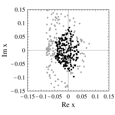
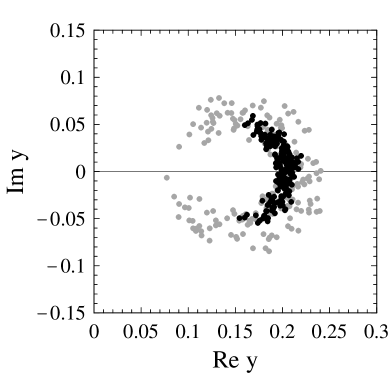
Figure 1: Real and imaginary parts of the quantities $x=\varepsilon_{a}\,e^{i(\eta-\phi)}$ (left) and $y=\varepsilon_{T}\,e^{i(\phi_{T}-\phi_{3/2})}$ (right) for different choices of hadronic parameters.

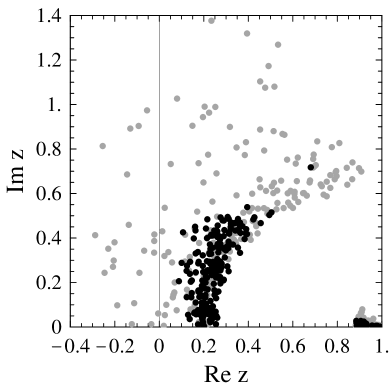
Figure 2: Real and imaginary parts of the quantity $z=(q_{C}/\delta_{+})\,e^{i\omega_{C}}$. The accumulation of points in the lower-right corner shows the corresponding results for the quantity $(q/\delta_{+})\,e^{i\omega}$. Only points with $\mbox{Im}\,z>0$ are shown.

For the strong-interaction phases we consider two sets of parameter choices: one which we believe is realistic and one which we think is very conservative. For the realistic set, we require that $0.5<\xi<1.5$, $|\phi_{3/2}-\phi_{1/2}^{(+)}|<45^{\circ}$, and $|\phi_{I}^{+}-\phi_{I}^{-}|<20^{\circ}$ (with $I=\frac{1}{2}$ or $\frac{3}{2}$). For the conservative set, we increase these ranges to $0<\xi<2$, $|\phi_{3/2}-\phi_{1/2}^{(+)}|<90^{\circ}$, and $|\phi_{I}^{+}-\phi_{I}^{-}|<45^{\circ}$. In our opinion, values outside these ranges are quite inconceivable. Note that, for the moment, no assumption is made about the relative strong-interaction phases of tree and penguin ampltiudes. We choose the various parameters randomly inside the allowed intervals and present the results for the quantities $\varepsilon_{a}\,e^{i\eta}$ in units of $e^{i\phi}$, $\varepsilon_{T}\,e^{i\phi_{T}}$ in units of $e^{i\phi_{3/2}}$, and $q_{(C)}\,e^{i\omega_{(C)}}$ in units of $\delta_{+}$ in the form of scatter plots in Figures 1 and 2. The black and the gray points correspond to the realistic and to the conservative parameter sets, respectively. The same colour coding will be used throughout this work.

The left-hand plot in Figure 1 shows that the parameter $\varepsilon_{a}$ generally takes rather small values. For the realistic parameter set we find $\varepsilon_{a}<0.08$, whereas values up tp 0.15 are possible for the conservative set. There is no strong correlation between the strong-interaction phases $\eta$ and $\phi$. An important implication of these observations is that, in general, there will be a very small difference between the quantities $\varepsilon_{3/2}$ and $\bar{\varepsilon}_{3/2}$ in (10). We shall therefore consider the same range of values for the two parameters. From the right-hand plot we observe that for realistic parameter choices $0.15<\varepsilon_{T}<0.22$; however, values between 0.08 and 0.24 are possible for the conservative parameter set. Note that there is a rather strong correlation between the strong-interaction phases $\phi_{T}$ and $\phi_{3/2}$, which differ by less than $20^{\circ}$ for the realistic parameter set. We will see in Section 5 that this implies a strong correlation between the direct CP asymmetries in the decays $B^{\pm}\to\pi^{0}K^{\pm}$ and $B^{0}\to\pi^{\mp}K^{\pm}$. Figure 2 shows that, even for the realistic parameter set, the ratio $q_{C}/\delta_{+}$ can be substantially larger than the naive expectation of about 0.2. Indeed, values as large as 0.7 are possible, and for the conservative set the wide range $0<q_{C}/\delta_{+}<1.4$ is allowed. Likewise, the strong-interaction phase $\omega_{C}$ can naturally be large and take values of up to $75^{\circ}$ even for the realistic parameter set. (Note that, without loss of generality, only points with positive values of $\omega_{(C)}$ are displayed in the plot. The distribution is invariant under a change of the sign of the strong-interaction phase.) This is in stark contrast to the case of the quantity $q\,e^{i\omega}$ entering the isospin amplitude $A_{3/2}$, where both the magnitude $q$ and the phase $\omega$ are determined within very small uncertainties, as is evident from the figure.

3 Hadronic uncertainties in the Fleischer–Mannel bound

As a first phenomenological application of the results of the previous section, we investigate the effects of rescattering and electroweak penguin contributions on the Fleischer–Mannel bound on $\gamma$ derived from the ratio $R$ defined in (2). In general, $R\neq 1$ because the parameter $\varepsilon_{T}$ in (9) does not vanish. To leading order in the small quantities $\varepsilon_{i}$, we find

$$R\simeq 1-2\varepsilon_{T}\Big{[}\cos\tilde{\phi}\cos\gamma-q_{C}\cos(\tilde{\phi}+\omega_{C})\Big{]}+O(\varepsilon_{i}^{2})\,,$$ (42)

where $\tilde{\phi}=\phi_{T}-\phi_{P}$. Because of the uncertainty in the values of the hadronic parameters $\varepsilon_{T}$, $q_{C}$ and $\omega_{C}$, it is difficult to convert this result into a constraint on $\gamma$. Fleischer and Mannel have therefore suggested to derive a lower bound on the ratio $R$ by eliminating the parameter $\varepsilon_{T}$ from the exact expression for $R$. In the limit where $\varepsilon_{a}$ and $q_{C}$ are set to zero, this yields $R\geq\sin^{2}\!\gamma$ [3]. However, this simple result must be corrected in the presence of rescattering effects and electroweak penguin contributions. The generalization is [9]

$$R\geq\frac{1-2q_{C}\,\varepsilon_{a}\cos(\omega_{C}+\eta)+q_{C}^{2}\,\varepsilon_{a}^{2}}{(1-2q_{C}\cos\omega_{C}\cos\gamma+q_{C}^{2})(1-2\varepsilon_{a}\cos\eta\cos\gamma+\varepsilon_{a}^{2})}\,\sin^{2}\!\gamma\,.$$ (43)

The most dangerous rescattering effects arise from the terms involving the electroweak penguin parameter $q_{C}$. As seen from Figure 2, even restricting ourselves to the realistic parameter set we can have $2q_{C}\cos\omega_{C}\approx\delta_{+}\approx 0.7$ and $q_{C}^{2}\approx 0.5\,\delta_{+}^{2}\approx 0.2$, implying that the quadratic term in the denominator by itself can give a 20% correction. The rescattering effects parametrized by $\varepsilon_{a}$ are presumably less important.

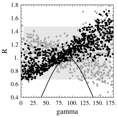
Figure 3: Results for the ratio $R$ versus $|\gamma|$ (in degrees) for different choices of hadronic parameters. The curve shows the minimal value $R_{\rm min}=\sin^{2}\!\gamma$ corresponding to the Fleischer–Mannel bound. The band shows the current experimental value of $R$ with its $1\sigma$ variation.

The results of the numerical analysis are shown in Figure 3. In addition to the parameter choices described in Section 2.6, we vary $\varepsilon_{3/2}$ and $\delta_{+}$ in the ranges $0.24\pm 0.06$ and $0.68\pm 0.11$, respectively. Now also the relative strong-interaction phase $\phi$ between the penguin and $I=\frac{3}{2}$ tree amplitudes enters. We allow values $|\phi|<90^{\circ}$ for the realistic parameter set, and impose no constraint on $\phi$ at all for the conservative parameter set. The figure shows that the corrections to the Fleischer–Mannel bound are not as large as suggested by the result (43), the reason being that this result is derived allowing arbitrary values of $\varepsilon_{T}$, whereas in our analysis the allowed values for this parameter are constrained. However, there are sizable violations of the naive bound $R<\sin^{2}\!\gamma$ for $|\gamma|$ in the range between $65^{\circ}$ and $125^{\circ}$, which includes most of the region $47^{\circ}<\gamma<105^{\circ}$ preferred by the global analysis of the unitarity triangle [32]. Whereas these violations are numerically small for the realistic parameter set, they can become large for the conservative set, because then a large value of the phase difference $|\phi_{3/2}-\phi_{1/2}^{+}|$ is allowed [6]. We conclude that under conservative assumptions only for values $R<0.8$ a constraint on $\gamma$ can be derived

Fleischer has argued that one can improve upon the above analysis by extracting some of the unknown hadronic parameters $q_{C}$, $\varepsilon_{a}$, $\omega_{C}$ and $\eta$ from measurements of other decay processes [9]. The idea is to combine information on the ratio $R$ with measurements of the direct CP asymmetries in the decays $B^{0}\to\pi^{\mp}K^{\pm}$ and $B^{\pm}\to\pi^{\pm}K^{0}$, as well as of the ratio $R_{K}$ defined in (33). One can then derive a bound on $R$ that depends, besides the electroweak penguin parameters $q_{C}$ and $\omega_{C}$, only on a combination $w=w(\varepsilon_{a},\eta)$, which can be determined up to a two-fold ambiguity assuming SU(3) flavour symmetry. Besides the fact that this approach relies on SU(3) symmetry and involves significantly more experimental input than the original Fleischer–Mannel analysis, it does not allow one to eliminate the theoretical uncertainty related to the presence of electroweak penguin contributions.

4 Hadronic uncertainties in the $R_{*}$ bound

As a second application, we investigate the implications of recattering effects on the bound on $\cos\gamma$ derived from a measurement of the ratio $R_{*}$ defined in (2). In this case, the theoretical analysis is cleaner because there is model-independent information on the values of the hadronic parameters $\varepsilon_{3/2}$, $q$ and $\omega$ entering the parametrization of the isospin amplitude $A_{3/2}$ in (9). The important point noted in [10] is that the decay amplitudes for $B^{\pm}\to\pi^{\pm}K^{0}$ and $B^{\pm}\to\pi^{0}K^{\pm}$ differ only in this single isospin amplitude. Since the overall strength of $A_{3/2}$ is governed by the parameter $\bar{\varepsilon}_{3/2}$ and thus can be determined from experiment without much uncertainty, we have suggested to derive a bound on $\cos\gamma$ without eliminating this parameter. In this respect, our strategy is different from the Fleischer–Mannel analysis.

The exact theoretical expression for the inverse of the ratio $R_{*}$ is given by

$$R_{*}^{-1} = 1+2\bar{\varepsilon}_{3/2}\,\frac{\cos\phi\,(\delta_{\rm EW}-\cos\gamma)+\varepsilon_{a}\cos(\phi-\eta)(1-\delta_{\rm EW}\cos\gamma)}{\sqrt{1-2\varepsilon_{a}\cos\eta\cos\gamma+\varepsilon_{a}^{2}}}$$ (44)

$$\mbox{}+\bar{\varepsilon}_{3/2}^{2}(1-2\delta_{\rm EW}\cos\gamma+\delta_{\rm EW}^{2})\,,$$

where $\bar{\varepsilon}_{3/2}$ has been defined in (10). Relevant for the bound on $\cos\gamma$ is the maximal value $R_{*}^{-1}$ can take for fixed $\gamma$. In [10], we have worked to linear order in the parameters $\varepsilon_{i}$, so that terms proportional to $\varepsilon_{a}$ could be neglected. Here, we shall generalize the discussion and keep all terms exactly. Varying the strong-interaction phases $\phi$ and $\eta$ independently, we find that the maximum value of $R_{*}^{-1}$ is given by

$$R_{*}^{-1}\leq 1+2\bar{\varepsilon}_{3/2}\,\frac{|\delta_{\rm EW}-\cos\gamma\pm\varepsilon_{a}(1-\delta_{\rm EW}\cos\gamma)|}{\sqrt{1\mp 2\varepsilon_{a}\cos\gamma+\varepsilon_{a}^{2}}}+\bar{\varepsilon}_{3/2}^{2}(1-2\delta_{\rm EW}\cos\gamma+\delta_{\rm EW}^{2})\,,$$ (45)

where the upper (lower) signs apply if $\cos\gamma<c_{0}$ ($\cos\gamma>c_{0}$) with

$$c_{0}=\frac{(1+\varepsilon_{a}^{2})\,\delta_{\rm EW}}{1+\varepsilon_{a}^{2}\,\delta_{\rm EW}^{2}}\simeq\delta_{\rm EW}\,.$$ (46)

Keeping all terms in $\bar{\varepsilon}_{3/2}$ exactly, but working to linear order in $\varepsilon_{a}$, we find the simpler result

$$R_{*}^{-1}\leq\Big{(}1+\bar{\varepsilon}_{3/2}\,|\delta_{\rm EW}-\cos\gamma|\Big{)}^{2}+\bar{\varepsilon}_{3/2}(\bar{\varepsilon}_{3/2}+2\varepsilon_{a})\sin^{2}\!\gamma+O(\bar{\varepsilon}_{3/2}\,\varepsilon_{a}^{2})\,.$$ (47)

The higher-order terms omitted here are of order 1% and thus negligible. The annihilation contribution $\varepsilon_{a}$ enters this result in a very transparent way: increasing $\varepsilon_{a}$ increases the maximal value of $R_{*}^{-1}$ and therefore weakens the bound on $\cos\gamma$.

In [10], we have introduced the quantity $\Delta_{*}$ by writing $R_{*}=(1-\Delta_{*})^{2}$, so that $\Delta_{*}=1-\sqrt{R_{*}}$ obeys the bound shown in (3). Note that to first order in $\bar{\varepsilon}_{3/2}$ the rescattering contributions proportional to $\varepsilon_{a}$ do not enter. Armed with the result (45), we can now derive the exact expression for the maximal value of the quantity $\Delta_{*}$, corresponding to the minimal value of $R_{*}$. It is of advantage to consider the ratio $\Delta_{*}/\bar{\varepsilon}_{3/2}$, the bound for which is to first order independent of the parameter $\bar{\varepsilon}_{3/2}$. We recall that this ratio can be determined experimentally up to nonfactorizable SU(3)-breaking corrections. Its current value is $\Delta_{*}/\bar{\varepsilon}_{3/2}=1.33\pm 0.78$.

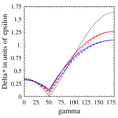
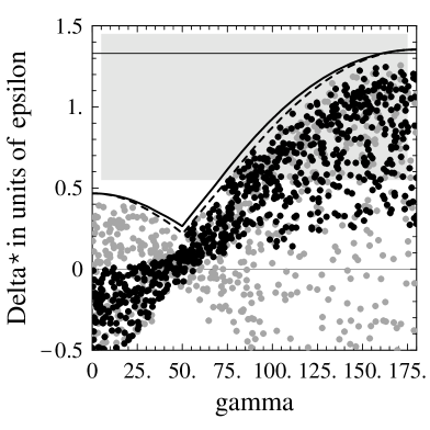
Figure 4: Left: Theoretical upper bound on the ratio $\Delta_{*}/\bar{\varepsilon}_{3/2}$ versus $|\gamma|$ for various choices of $\bar{\varepsilon}_{3/2}$ and $\varepsilon_{a}$, as explained in the text. The dotted line shows the linear bound derived in [10]. Right: Results for this ratio obtained for different choices of hadronic parameters. The curves show the theoretical bound for $\varepsilon_{a}=0.1$ (solid) and $\varepsilon_{a}=0$ (dashed). The band shows the current experimental value with its $1\sigma$ variation.

In the left-hand plot in Figure 4, we show the maximal value for the ratio $\Delta_{*}/\bar{\varepsilon}_{3/2}$ for different values of the parameters $\bar{\varepsilon}_{3/2}$ and $\varepsilon_{a}$. The upper (red) and lower (blue) pairs of curves correspond to $\bar{\varepsilon}_{3/2}=0.18$ and 0.30, respectively, and span the allowed range of values for this parameter. For each pair, the dashed and solid lines correspond to $\varepsilon_{a}=0$ and 0.1, respectively. To saturate the bound (45) requires to have $\eta-\phi=0^{\circ}$ or $180^{\circ}$, in which case $\varepsilon_{a}=0.1$ is a conservative upper limit (see Figure 1). The dotted curve shows for comparison the linearized result obtained by neglecting the higher-order terms in (3). The parameter $\delta_{\rm EW}=0.64$ is kept fixed in this plot. As expected, the bound on the ratio $\Delta_{*}/\bar{\varepsilon}_{3/2}$ is only weakly dependent on the values of $\bar{\varepsilon}_{3/2}$ and $\varepsilon_{a}$. In particular, not much is lost by using the conservative value $\varepsilon_{a}=0.1$. Note that for values $\Delta_{*}/\bar{\varepsilon}_{3/2}>0.8$ the linear bound (3) is conservative, i.e., weaker than the exact bound, and even for smaller values of $\Delta_{*}/\bar{\varepsilon}_{3/2}$ the violations of this bound are rather small. Expanding the exact bound to next-to-leading order in $\bar{\varepsilon}_{3/2}$, we obtain

$$\frac{\Delta_{*}}{\bar{\varepsilon}_{3/2}}\leq|\delta_{\rm EW}-\cos\gamma|-\bar{\varepsilon}_{3/2}\left[\left(\frac{\Delta_{*}}{\bar{\varepsilon}_{3/2}}\right)^{2}-\left(\frac{1}{2}+\frac{\varepsilon_{a}}{\bar{\varepsilon}_{3/2}}\right)\sin^{2}\!\gamma\right]+O(\bar{\varepsilon}_{3/2}^{2})\,,$$ (48)

showing that $\Delta_{*}/\bar{\varepsilon}_{3/2}>(1/2+\varepsilon_{a}/\bar{\varepsilon}_{3/2})^{1/2}$ is a criterion for the validity of the linearized bound. This generalizes a condition derived, for the special case $\varepsilon_{a}\ll\bar{\varepsilon}_{3/2}$, in [10].

To obtain a reliable bound on the weak phase $\gamma$, we must account for the theoretical uncertainty in the value of the electroweak penguin parameter $\delta_{\rm EW}$ in the Standard Model, which is however straightforward to do by lowering (increasing) the value of this parameter used in calculating the right (left) branch of the curves defining the bound. The solid line in the right-hand plot in Figure 4 shows the most conservative bound obtained by using $\varepsilon_{a}=0.1$ and varying the other two parameters in the ranges $0.18<\bar{\varepsilon}_{3/2}<0.30$ and $0.49<\delta_{\rm EW}<0.79$. The scatter plot shows the distribution of values of $\Delta_{*}/\bar{\varepsilon}_{3/2}$ obtained by scanning the strong-interaction parameters over the same ranges as we did for the Fleischer–Mannel case in the previous section. The horizontal band shows the current central experimental value with its $1\sigma$ variation. Unlike the Fleischer–Mannel bound, there is no violation of the bound (by construction), since all parameters are varried over conservative ranges. Indeed, for the points close to the right branch of the bound $\eta-\phi=0^{\circ}$, so that according to Figure 1 almost all of these points have $\varepsilon_{a}<0.03$, which is smaller than the value we used to obtain the theoretical curve. The dashed curve shows the bound for $\varepsilon_{a}=0$, which is seen not to be violated by any point. This shows that the rescattering effects parametrized by the quantity $\varepsilon_{a}$ play a very minor role in the bound derived from the ratio $R_{*}$. We conclude that, if the current experimental value is confirmed to within one standard deviation, i.e., if future measurements find that $\Delta_{*}/\bar{\varepsilon}_{3/2}>0.55$, this would imply the bound $|\gamma|>75^{\circ}$, which is very close to the value of $77^{\circ}$ obtained in [10].

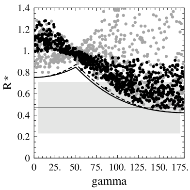
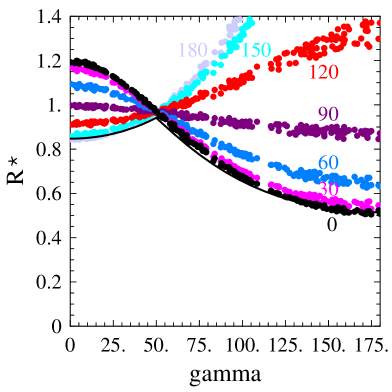
Figure 5: Left: Results for the ratio $R_{*}$ obtained for different choices of hadronic parameters. The curves show the theoretical bound for $\varepsilon_{a}=0.1$ (solid) and $\varepsilon_{a}=0$ (dashed). The band shows the current experimental value of $R_{*}$ with its $1\sigma$ variation. Right: Results for the ratio $R_{*}$ for different values of the strong-interaction phase $|\phi|$, as indicated by the numbers.

Given that the experimental determination of the parameter $\bar{\varepsilon}_{3/2}$ is limited by unknown nonfactorizable SU(3)-breaking corrections, one may want to be more conservative and derive a bound directly from the measured ratio $R_{*}$ rather than the ratio $\Delta_{*}/\bar{\varepsilon}_{3/2}$. In the left-hand plot in Figure 5, we show the same distribution as in the right-hand plot in Figure 4, but now for the ratio $R_{*}$. The resulting bound on $\gamma$ is slightly weaker, because now there is a stronger dependence on the value of $\bar{\varepsilon}_{3/2}$, which we vary as previously between 0.18 and 0.30. If the current value of $R_{*}$ is confimed to within one standard deviation, i.e., if future measurements find that $R_{*}<0.71$, this would imply the bound $|\gamma|>72^{\circ}$.

Besides providing interesting information on $\gamma$, a measurement of $R_{*}$ or $\Delta_{*}/\bar{\varepsilon}_{*}$ can yield information about the strong-interaction phase $\phi$. In the right plot in Figure 5, we show the distribution of points obtained for fixed values of the strong-interaction phase $|\phi|$ between $0^{\circ}$ and $180^{\circ}$ in steps of $30^{\circ}$. For simplicity, the parameters $\varepsilon_{3/2}=0.24$ and $\delta_{\rm EW}=0.64$ are kept fixed in this plot, while all other hadronic parameters are scanned over the realistic parameter set. We observe that, independently of $\gamma$, a value $R_{*}<0.8$ requires that $|\phi|<90^{\circ}$. This conclusion remains true if the parameters $\varepsilon_{3/2}$ and $\delta_{\rm EW}$ are varied over their allowed ranges. We shall study the correlation between the weak phase $\gamma$ and the strong phase $\phi$ in more detail in Section 6.

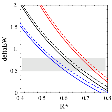
Figure 6: Lower bound on the parameter $\delta_{\rm EW}$ as a function of $R_{*}$. The upper (red), middle (black) and lower (blue) curves correspond to $\bar{\varepsilon}_{3/2}=0.18$, 0.24 and 0.30, respectively. The solid and dashed lines refer to $\varepsilon_{a}=0.1$ and 0. The band shows the prediction for $\delta_{\rm EW}$ in the Standard Model.

Finally, we emphasize that a future, precise measurement of the ratio $R_{*}$ may also yield a surprise and indicate physics beyond the Standard Model. The global analysis of the unitarity triangle requires that $|\gamma|<105^{\circ}$ [32], for which the lowest possible value of $R_{*}$ in the Standard Model is about 0.55. If the experimental value would turn out to be less than that, this would be strong evidence for New Physics. In particular, in many extensions of the Standard Model there would be additional contributions to the electroweak penguin parameter $\delta_{\rm EW}$ arising, e.g., from penguin and box diagrams containing new charged Higgs bosons. This could explain a larger value of $R_{*}$. Indeed, from (47) we can derive the bound

$$\delta_{\rm EW}\! \geq \!\frac{\sqrt{R_{*}^{-1}-\bar{\varepsilon}_{3/2}(\bar{\varepsilon}_{3/2}+2\varepsilon_{a})\sin^{2}\!\gamma_{\rm max}}-1}{\bar{\varepsilon}_{3/2}}$$ (49)

$$\mbox{}+\cos\gamma_{\rm max}\,,$$

where $\gamma_{\rm max}$ is the maximal value allowed by the global analysis (assuming that $\gamma_{\rm max}>\arccos(c_{0})\approx 50^{\circ}$). In Figure 6, we show this bound for the current value $\gamma_{\rm max}=105^{\circ}$ and three different values of $\bar{\varepsilon}_{3/2}$ as well as two different values of $\varepsilon_{a}$. The gray band shows the allowed range for $\delta_{\rm EW}$ in the Standard Model. In the hypothetical situation where the current central values $R_{*}=0.47$ and $\bar{\varepsilon}_{3/2}=0.24$ would be confirmed by more precise measurements, we would conclude that the value of $\delta_{\rm EW}$ is at least twice as large as predicted by the Standard Model.

5 Prospects for direct CP asymmetries and prediction for the
$B^{0}\to\pi^{0}K^{0}$ branching ratio

5.1 Decays of charged $B$ mesons

We will now analyse the potential of the various $B\to\pi K$ decay modes for showing large direct CP violation, starting with the decays of charged $B$ mesons. The smallness of the rescattering effects parametrized by $\varepsilon_{a}$ (see Figure 1) combined with the simplicity of the isospin amplitude $A_{3/2}$ (see Section 2.3) make these processes particularly clean from a theoretical point of view.

Explicit expressions for the CP asymmetries in the various decays can be derived in a straightforward way starting from the isospin decomposition in (6) and inserting the parametrizations for the isospin amplitudes derived in Section 2. The result for the CP asymmetry in the decays $B^{\pm}\to\pi^{\pm}K^{0}$ has already been presented in (31). The corresponding expression for the decays $B^{\pm}\to\pi^{0}K^{\pm}$ reads

$$A_{\rm CP}(\pi^{0}K^{+})=2\sin\gamma\,R_{*}\,\frac{\varepsilon_{3/2}\sin\phi+\varepsilon_{a}\sin\eta-\varepsilon_{3/2}\,\varepsilon_{a}\,\delta_{\rm EW}\sin(\phi-\eta)}{1-2\varepsilon_{a}\cos\eta\cos\gamma+\varepsilon_{a}^{2}}\,,$$ (50)

where the theoretical expression for $R_{*}$ is given in (44), and we have not replaced $\varepsilon_{3/2}$ in terms of $\bar{\varepsilon}_{3/2}$. Neglecting terms of order $\varepsilon_{a}$ and working to first order in $\varepsilon_{3/2}$, we find the estimate $A_{\rm CP}(\pi^{0}K^{+})\simeq 2\varepsilon_{3/2}\sin\gamma\sin\phi\approx 0.5\sin\gamma\sin\phi$, indicating that potentially there could be a very large CP asymmetry in this decay (note that $\sin\gamma>0.73$ is required by the global analysis of the unitarity triangle).

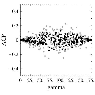
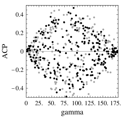
Figure 7: Results for the direct CP asymmetries $A_{\rm CP}(\pi^{+}K^{0})$ (left) and $A_{\rm CP}(\pi^{0}K^{+})$ (right) versus $|\gamma|$.

In Figure 7, we show the results for the two direct CP asymmetries in (31) and (50), both for the realistic and for the conservative parameter sets. These results confirm the general observations made above. For the realistic parameter set, and with $\gamma$ between $47^{\circ}$ and $105^{\circ}$ as indicated by the global analysis of the unitarity triangle [32], we find CP asymmetries of up to 15% in $B^{\pm}\to\pi^{\pm}K^{0}$ decays, and of up to 50% in $B^{\pm}\to\pi^{0}K^{\pm}$ decays. Of course, to have large asymmetries requires that the sines of the strong-interaction phases $\eta$ and $\phi$ are not small. However, this is not unlikely to happen. According to the left-hand plot in Figure 1, the phase $\eta$ can take any value, and the phase $\phi$ could quite conceivably be large due to the different decay mechanisms of tree- and penguin-initiated processes. We stress that there is no strong correlation between the CP asymmetries in the two decay processes, because as shown in Figure 1 there is no such correlation between the strong-interaction phases $\eta$ and $\phi$.

5.2 Decays of neutral $B$ mesons

Because of their dependence on the hadronic parameters $\varepsilon_{T}$, $q_{C}$ and $\omega_{C}$ entering through the sum $A_{1/2}+A_{3/2}$ of isospin amplitudes, the theoretical analysis of neutral $B\to\pi K$ decays is affected by larger hadronic uncertainties than that of the decays of charged $B$ mesons. Nevertheless, some interesting predictions regarding neutral $B$ decays can be made and tested experimentally.

The expression for the direct CP asymmetry in the decays $B^{0}\to\pi^{\mp}K^{\pm}$ is

$$A_{\rm CP}(\pi^{-}K^{+})=\frac{2\sin\gamma}{R}\,\frac{\varepsilon_{T}(\sin\tilde{\phi}-\varepsilon_{T}\,q_{C}\sin\omega_{C})+\varepsilon_{a}\,[\sin\eta-\varepsilon_{T}\,q_{C}\sin(\tilde{\phi}-\eta+\omega_{C})]}{1-2\varepsilon_{a}\cos\eta\cos\gamma+\varepsilon_{a}^{2}}\,,$$ (51)

where $\tilde{\phi}=\phi_{T}-\phi_{P}$. This result reduces to (50) under the replacements $q_{C}\to\delta_{\rm EW}$, $\omega_{C}\to 0$, $R\to R_{*}^{-1}$, and $\varepsilon_{T}\to\varepsilon_{3/2}$. The corresponding expression for the direct CP asymmetry in the decays $B^{0}\to\pi^{0}K^{0}$ and $\bar{B}^{0}\to\pi^{0}\bar{K}^{0}$ is more complicated and will not be presented here. Below, we shall derive an exact relation between the various asymmetries, which can be used to compute $A_{\rm CP}(\pi^{0}K^{0})$.

Gronau and Rosner have emphasized that one expects $A_{\rm CP}(\pi^{-}K^{+})\approx A_{\rm CP}(\pi^{0}K^{+})$, and that one could thus combine the data samples for these decays to enhance the statistical significance of an early signal of direct CP violation [36]. We can easily understand the argument behind this observation using our results. Neglecting the small rescattering contributions proportional to $\varepsilon_{a}$ for simplicity, we find

$$\frac{A_{\rm CP}(\pi^{-}K^{+})}{A_{\rm CP}(\pi^{0}K^{+})}\simeq\frac{1}{R_{*}R}\,\frac{\varepsilon_{T}(\sin\tilde{\phi}-\varepsilon_{T}\,q_{C}\sin\omega_{C})}{\varepsilon_{3/2}\sin\phi}\simeq\frac{1}{R_{*}R}\,\frac{\varepsilon_{T}}{\varepsilon_{3/2}}\,.$$ (52)

In the last step, we have used that the electroweak penguin contribution is very small because it is suppressed by an additional factor of $\varepsilon_{T}$, and that the strong-interaction phases $\phi$ and $\tilde{\phi}$ are strongly correlated, as follows from the right-hand plot in Figure 1. Numerically, the right-hand side turns out to be close to 1 for most of parameter space. This is evident from the left-hand plot in Figure 8, which confirms that there is indeed a very strong correlation between the CP asymmetries in the decays $B^{0}\to\pi^{\mp}K^{\pm}$ and $B^{\pm}\to\pi^{0}K^{\pm}$, in agreement with the argument given in [36]. Combining the data samples for these decays collected by the CLEO experiment, one may have a chance for observing a statistically significant signal for the first direct CP asymmetry in $B$ decays before the operation of the asymmetric $B$ factories.

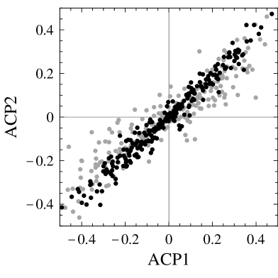
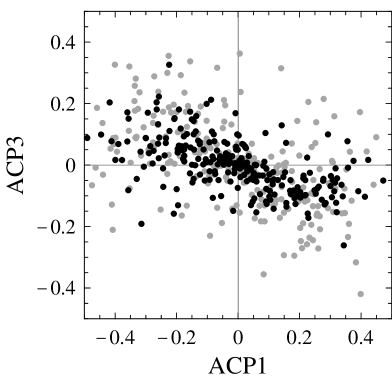
Figure 8: Correlation between the direct CP asymmetries $\mbox{ACP1}=A_{\rm CP}(\pi^{0}K^{+})$, $\mbox{ACP2}=A_{\rm CP}(\pi^{-}K^{+})$, and $\mbox{ACP3}=A_{\rm CP}(\pi^{0}K^{0})$.

The decays $B^{0}\to\pi^{0}K^{0}$ and $\bar{B}^{0}\to\pi^{0}\bar{K}^{0}$ have not yet been observed experimentally, but the CLEO Collaboration has presented an upper bound on their CP-averaged branching ratio of $4.1\times 10^{-5}$ [1]. In analogy with (2), we define the ratios

$$R_{0} = \frac{\tau(B^{+})}{\tau(B^{0})}\,\frac{2[\mbox{Br}(B^{0}\to\pi^{0}K^{0})+\mbox{Br}(\bar{B}^{0}\to\pi^{0}\bar{K}^{0})]}{\mbox{Br}(B^{+}\to\pi^{+}K^{0})+\mbox{Br}(B^{-}\to\pi^{-}\bar{K}^{0})}\,,$$

$$R_{0*} = \frac{2[\mbox{Br}(B^{0}\to\pi^{0}K^{0})+\mbox{Br}(\bar{B}^{0}\to\pi^{0}\bar{K}^{0})]}{\mbox{Br}(B^{0}\to\pi^{-}K^{+})+\mbox{Br}(\bar{B}^{0}\to\pi^{+}K^{-})}=\frac{R_{0}}{R}\,.$$ (53)

Using our parametrizations for the different isospin amplitudes, we find that the ratios $R$, $R_{*}$ and $R_{0}$ obey the relations

$$R_{0}-R+R_{*}^{-1}-1=\Delta_{1}\,,\qquad R_{0}-R\,R_{*}=\Delta_{2}+O(\bar{\varepsilon}_{i}^{3})\,,$$ (54)

where

$$\Delta_{1} = 2\bar{\varepsilon}_{3/2}^{2}\,(1-2\delta_{\rm EW}\cos\gamma+\delta_{\rm EW}^{2})-2\bar{\varepsilon}_{3/2}\,\bar{\varepsilon}_{T}\,(1-\delta_{\rm EW}\cos\gamma)\cos(\phi_{T}-\phi_{3/2})$$

$$\mbox{}-2\bar{\varepsilon}_{3/2}\,\bar{\varepsilon}_{T}\,q_{C}\,(\delta_{\rm EW}-\cos\gamma)\cos(\phi_{T}-\phi_{3/2}+\omega_{C})\,,$$

$$\Delta_{2} = \Delta_{1}-4\bar{\varepsilon}_{3/2}^{2}(\delta_{\rm EW}-\cos\gamma)^{2}\cos^{2}\!\phi$$ (55)

$$\mbox{}+4\bar{\varepsilon}_{3/2}\,\bar{\varepsilon}_{T}\,(\delta_{\rm EW}-\cos\gamma)\cos\phi\left[q_{C}\cos(\tilde{\phi}+\omega_{C})-\cos\gamma\cos\tilde{\phi}\right]\,,$$

and $\bar{\varepsilon}_{T}$ is defined in analogy with $\bar{\varepsilon}_{3/2}$ in (10), so that $\bar{\varepsilon}_{T}/\varepsilon_{T}=\bar{\varepsilon}_{3/2}/\varepsilon_{3/2}$. The first relation in (54) generalizes a sum rule derived by Lipkin, who neglected the terms of $O(\varepsilon_{i}^{2})$ on the right-hand side as well as electroweak penguin contributions [37]. The second relation is new. It follows from the fact that $R_{0*}=R_{*}+O(\varepsilon_{i}^{2})$, which is evident since the pairs of decay amplitudes entering the definition of the two ratios differ only in the isospin amplitude $A_{3/2}$.

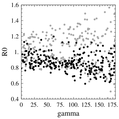
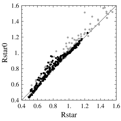
Figure 9: Ratio $R_{0}$ (left), and correlation between the ratios $R_{*}$ and $R_{0*}$ (right).

The left-hand plot in Figure 9 shows the results for the ratio $R_{0}$ versus $|\gamma|$. The dependence of this ratio on the weak phase turns out to be much weaker than in the case of the ratios $R$ and $R_{*}$. For the realistic parameter set we find that $0.7<R_{0}<1.0$ for most choices of strong-interaction parameters. Combining this with the current value of the $B^{\pm}\to\pi^{\pm}K^{0}$ branching ratio, we obtain values between $(0.47\pm 0.18)\times 10^{-5}$ and $(0.67\pm 0.26)\times 10^{-5}$ for the CP-averaged $B^{0}\to\pi^{0}K^{0}$ branching ratio. The right-hand plot in Figure 9 shows the strong correlation between the ratios $R_{*}$ and $R_{0*}=R_{0}/R$, which holds with a remarkable accuracy over all of parameter space.

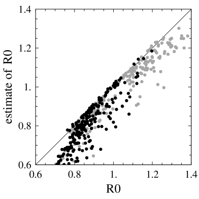
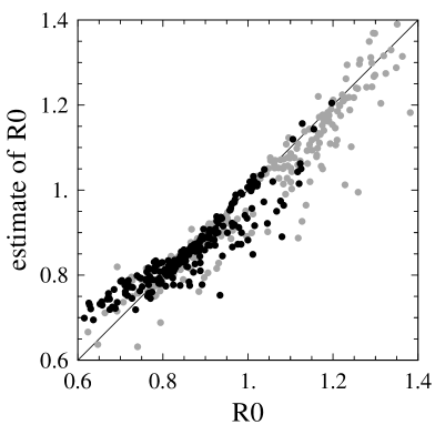
Figure 10: Esimates of $R_{0}$ obtained using the first (left) and second (right) sum rule in (54).

In Figure 10, we show the estimates of $R_{0}$ obtained by neglecting the terms of $O(\bar{\varepsilon}_{i}^{2})$ and higher in the two sum rules in (54). Using the present data for the various branching ratios yields to the estimates $R_{0}=(-0.1\pm 0.9)$ from the first and $R_{0}=(0.5\pm 0.2)$ from the second sum rule. Both results are consistent with the theoretical expectations for $R_{0}$ exhibited in the left-hand plot in Figure 9; however, the second estimate has a much smaller experimental error and, according to Figure 10, it is likely to have a higher theoretical accuracy. We can rewrite this estimate as

$$\frac{1}{2}\Big{[}\mbox{Br}(B^{0}\to\pi^{0}K^{0})+\mbox{Br}(\bar{B}^{0}\to\pi^{0}\bar{K}^{0})\Big{]}\simeq\frac{\mbox{Br}(B^{\pm}\to\pi^{\pm}K^{0})\,\mbox{Br}(B^{0}\to\pi^{\mp}K^{\pm})}{4\mbox{Br}(B^{\pm}\to\pi^{0}K^{\pm})}\,,$$ (56)

where the branching ratios on the right-hand side are averaged over CP-conjugate modes. With current data, this relation yields the value $(0.33\pm 0.18)\times 10^{-5}$. Combining the three estimates for the CP-averaged $B^{0}\to\pi^{0}K^{0}$ branching ratio presented above we arrive at the value $(0.5\pm 0.2)\times 10^{-5}$, which is about a factor of 3 smaller than the other three $B\to\pi K$ branching ratios quoted in (1).

We now turn to the study of the direct CP asymmetry in the decays $B^{0}\to\pi^{0}K^{0}$ and $\bar{B}^{0}\to\pi^{0}\bar{K}^{0}$. Using our general parametrizations, we find the sum rule

$$A_{\rm CP}(\pi^{+}K^{0})-R_{*}^{-1}\,A_{\rm CP}(\pi^{0}K^{+})+R\,A_{\rm CP}(\pi^{-}K^{+})-R_{0}\,A_{\rm CP}(\pi^{0}K^{0})$$

$$\quad=2\sin\gamma\,\bar{\varepsilon}_{3/2}\,\bar{\varepsilon}_{T}\left[\delta_{\rm EW}\sin(\phi_{T}-\phi_{3/2})-q_{C}\sin(\phi_{T}-\phi_{3/2}+\omega_{C})\right]\,.$$ (57)

By scanning all strong-interaction parameters, we find that for the realistic (conservative) parameter set the right-hand side takes values of less that 4% (7%) times $\sin\gamma$ in magnitude. Neglecting these small terms, and using the approximate equality of the CP asymmetries in $B^{\pm}\to\pi^{0}K^{\pm}$ and $B^{0}\to\pi^{\mp}K^{\pm}$ decays as well as the second relation in (54), we obtain

$$A_{\rm CP}(\pi^{0}K^{0})\simeq-\frac{1-R\,R_{*}}{R\,R_{*}^{2}}\,A_{\rm CP}(\pi^{0}K^{+})+\frac{A_{\rm CP}(\pi^{+}K^{0})}{R\,R_{*}}\,.$$ (58)

The first term is negative for most choices of parameters and would dominate if the CP aymmetry in $B^{\pm}\to\pi^{0}K^{\pm}$ decays would turn out to be large. We therefore expect a weak anticorrelation between $A_{\rm CP}(\pi^{0}K^{0})$ and $A_{\rm CP}(\pi^{+}K^{0})$, which is indeed exhibited in the right-hand plot in Figure 9.

For completeness, we note that in the decays $B^{0}$, $\bar{B}^{0}\to\pi^{0}K_{S}$ one can also study mixing-induced CP violation, as has been emphasized recently in [11]. Because of the large hadronic uncertainties inherent in the calculation of this effect, we do not study this possibility further.

6 Determination of $\gamma$ from $B^{\pm}\to\pi K$, $\pi\pi$ decays

Ultimately, one would like not only to derive bounds on the weak phase $\gamma$, but to measure this parameter from a study of CP violation in $B\to\pi K$ decays. However, as we have pointed out in Section 2, this is not a trivial undertaking because even perfect measurements of all eight $B\to\pi K$ branching ratios would not suffice to eliminate all hadronic parameters entering the parametrization of the decay amplitudes.

Because of their theoretical cleanness, the decays of charged $B$ mesons are best suited for a measurement of $\gamma$. In [14], we have described a strategy for achieving this goal, which relies on the measurements of the CP-averaged branching ratios for the decays $B^{\pm}\to\pi^{\pm}K^{0}$ and $B^{\pm}\to\pi^{\pm}\pi^{0}$, as well as of the individual branching ratios for the decays $B^{+}\to\pi^{0}K^{+}$ and $B^{-}\to\pi^{0}K^{-}$, i.e., the direct CP asymmetry in this channel. This method is a generalization of the Gronau–Rosner–London (GRL) approach for extracting $\gamma$ [38]. It includes the contributions of electroweak penguin operators, which had previously been argued to spoil the GRL method [29, 39].

The strategy proposed in [14] relies on the dynamical assumption that there is no CP-violating contribution to the $B^{\pm}\to\pi^{\pm}K^{0}$ decay amplitudes, which is equivalent to saying that the rescattering effects parametrized by the quantity $\varepsilon_{a}$ in (8) are negligibly small. It is evident from the left-hand plot in Figure 1 that this assumption is indeed justified in a large region of parameter space. Here, we will refine the approach and investigate the theoretical uncertainty resulting from $\varepsilon_{a}\neq 0$. As a side product, we will show how nontrivial information on the strong-interaction phase difference $\phi=\phi_{3/2}-\phi_{P}$ can be obtained along with information on $\gamma$.

To this end, we consider in addition to the ratio $R_{*}$ the CP-violating observable

$$\widetilde{A}\equiv\frac{A_{\rm CP}(\pi^{0}K^{+})}{R_{*}}-A_{\rm CP}(\pi^{+}K^{0})=2\sin\gamma\,\bar{\varepsilon}_{3/2}\,\frac{\sin\phi-\varepsilon_{a}\,\delta_{\rm EW}\sin(\phi-\eta)}{\sqrt{1-2\varepsilon_{a}\cos\eta\cos\gamma+\varepsilon_{a}^{2}}}\,.$$ (59)

The purpose of subtracting the CP asymmetry in the decays $B^{\pm}\to\pi^{\pm}K^{0}$ is to eliminate the contribution of $O(\varepsilon_{a})$ in the expression for $A_{\rm CP}(\pi^{0}K^{+})$ given in (50). A measurement of this asymmetry is the new ingredient in our approach with respect to that in [14]. With the definition of $\widetilde{A}$ as given above, the rescattering effects parametrized by $\varepsilon_{a}$ are suppressed by an additional factor of $\bar{\varepsilon}_{3/2}$ and are thus expected to be very small. As shown in Section 4, the same is true for the ratio $R_{*}$. Explicitly, we have

$$R_{*}^{-1} = 1+2\bar{\varepsilon}_{3/2}\,\cos\phi\,(\delta_{\rm EW}-\cos\gamma)+\bar{\varepsilon}_{3/2}^{2}\,(1-2\delta_{\rm EW}\cos\gamma+\delta_{\rm EW}^{2})+O(\bar{\varepsilon}_{3/2}\,\varepsilon_{a})\,,$$

$$\widetilde{A} = 2\sin\gamma\,\bar{\varepsilon}_{3/2}\,\sin\phi+O(\bar{\varepsilon}_{3/2}\,\varepsilon_{a})\,.$$ (60)

These equations define contours in the $(\gamma,\phi)$ plane. When higher-order terms are kept, these contours become narrow bands, the precise shape of which depends on the values of the parameters $\bar{\varepsilon}_{3/2}$ and $\delta_{\rm EW}$. In the limit $\varepsilon_{a}=0$ the procedure described here is mathematically equivalent to the construction proposed in [14]. There, the errors on $\cos\gamma$ resulting from the variation of the input parameters have been discussed in detail. For a typical example, where $\gamma=76^{\circ}$ and $\phi=20^{\circ}$, we found that the uncertainties resulting from a 15% variation of $\bar{\varepsilon}_{3/2}$ and $\delta_{\rm EW}$ are $\cos\gamma=0.24\pm 0.09\pm 0.09$, correspondig to errors of $\pm 5^{\circ}$ each on the extracted value of $\gamma$.

Our focus here is to evaluate the additional uncertainty resulting from the rescattering effects parametrized by $\varepsilon_{a}$ and $\eta$. For given values of $\bar{\varepsilon}_{3/2}$, $\delta_{\rm EW}$, $\varepsilon_{a}$, $\eta$, and $\gamma$, the exact results for $R_{*}$ in (44) and $\widetilde{A}$ in (59) can be brought into the generic form $A\cos\phi+B\sin\phi=C$, where in the case of $R_{*}$

$$A = 2\bar{\varepsilon}_{3/2}\,\frac{\delta_{\rm EW}-\cos\gamma+\varepsilon_{a}\cos\eta\,(1-\delta_{\rm EW}\cos\gamma)}{\sqrt{1-2\varepsilon_{a}\cos\eta\cos\gamma+\varepsilon_{a}^{2}}}\,,$$

$$B = 2\bar{\varepsilon}_{3/2}\,\frac{\varepsilon_{a}\sin\eta\,(1-\delta_{\rm EW}\cos\gamma)}{\sqrt{1-2\varepsilon_{a}\cos\eta\cos\gamma+\varepsilon_{a}^{2}}}\,,$$

$$C = R_{*}^{-1}-1-\bar{\varepsilon}_{3/2}^{2}\,(1-2\delta_{\rm EW}\cos\gamma+\delta_{\rm EW}^{2})\,,$$ (61)

whereas for $\widetilde{A}$

$$A = 2\bar{\varepsilon}_{3/2}\,\frac{\varepsilon_{a}\,\delta_{\rm EW}\sin\eta}{\sqrt{1-2\varepsilon_{a}\cos\eta\cos\gamma+\varepsilon_{a}^{2}}}\,,$$

$$B = 2\bar{\varepsilon}_{3/2}\,\frac{1-\varepsilon_{a}\,\delta_{\rm EW}\cos\eta}{\sqrt{1-2\varepsilon_{a}\cos\eta\cos\gamma+\varepsilon_{a}^{2}}}\,,$$

$$C = \frac{\widetilde{A}}{\sin\gamma}\,.$$ (62)

The two solutions for $\cos\phi$ are given by

$$\cos\phi=\frac{AC\pm B\sqrt{A^{2}+B^{2}-C^{2}}}{A^{2}+B^{2}}\,.$$ (63)

The physical solutions must be such that $\cos\phi$ is real and its magnitude less than 1.

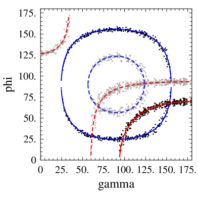
Figure 11: Contour plots for the quantities $R_{*}$ (red “hyperbolas”) and $\widetilde{A}$ (blue “circles”). The scatter plots show the results including rescattering effects, while the lines refer to $\varepsilon_{a}=0$. The solid curves correspond to the contours for $R_{*}=0.7$ and $\widetilde{A}=0.2$, the dashed ones to $R_{*}=0.9$ and $\widetilde{A}=0.4$.

In Figure 12, we show the resulting contour bands obtained by keeping $\bar{\varepsilon}_{3/2}=0.24$ and $\delta_{\rm EW}=0.64$ fixed to their central values, while the rescattering parameters are scanned over the ranges $0<\varepsilon_{a}<0.08$ and $-180^{\circ}<\eta<180^{\circ}$. Assuming that $\sin\gamma>0$ as suggested by the global analysis of the unitarity triangle, the sign of $\widetilde{A}$ determines the sign of $\sin\phi$. In the plot, we assume without loss of generality that $0^{\circ}\leq\phi\leq 180^{\circ}$. For instance, if $R_{*}=0.7$ and $\widetilde{A}=0.2$, then the two solutions are $(\gamma,\phi)\approx(98^{\circ},25^{\circ})$ and $(\gamma,\phi)\approx(153^{\circ},67^{\circ})$, only the first of which is allowed by the upper bound $\gamma<105^{\circ}$ following from the global analysis of the unitarity triangle [32]. It is evident that the contours are rather insensitive to the rescattering effects parametrized by $\varepsilon_{a}$ and $\eta$. The error on $\gamma$ due to these effects is about $\pm 5^{\circ}$, which is similar to the errors resulting from the theoretical uncertainties in the parameters $\bar{\varepsilon}_{3/2}$ and $\delta_{\rm EW}$. The combined theoretical uncertainty is of order $\pm 10^{\circ}$ on the extracted value of $\gamma$.

To summarize, the strategy for determining $\gamma$ would be as follows: From measurements of the CP-averaged branching ratio for the decays $B^{\pm}\to\pi^{\pm}\pi^{0}$, $B^{\pm}\to\pi^{\pm}K^{0}$ and $B^{\pm}\to\pi^{0}K^{\pm}$, the ratio $R_{*}$ and the parameter $\bar{\varepsilon}_{3/2}$ are determined using (2) and (4), respectively. Next, from measurements of the rate asymmetries in the decays $B^{\pm}\to\pi^{\pm}K^{0}$ and $B^{\pm}\to\pi^{0}K^{\pm}$ the quantity $\widetilde{A}$ is determined. From the contour plots for the quantities $R_{*}$ and $\widetilde{A}$ the phases $\gamma$ and $\phi$ can then be extracted up to discrete ambiguities. In this determination one must account for theoretical uncertainties in the values of the parameters $\bar{\varepsilon}_{3/2}$ and $\delta_{\rm EW}$, as well as for rescattering effects parametrized by $\varepsilon_{a}$ and $\eta$. Quantitative estimates for these uncertainties have been given above.

7 Conclusions

We have presented a model-independent, global analysis of the rates and direct CP asymmetries for the rare two-body decays $B\to\pi K$. The theoretical description exploits the flavour symmetries of the strong interactions and the structure of the low-energy effective weak Hamiltonian. Isospin symmetry is used to introduce a minimal set of three isospin amplitudes. The explicit form of the effective weak Hamiltonian in the Standard Model is used to simplify the isovector part of the interaction. Both the numerical smallness of certain Wilson coefficient functions and the Dirac and colour structure of the local operators are relevant in this context. Finally, the $U$-spin subgroup of flavour SU(3) symmetry is used to simplify the structure of the isospin amplitude $A_{3/2}$ referring to the decay $B\to(\pi K)_{I=3/2}$. In the limit of exact $U$-spin symmetry, two of the four parameters describing this amplitude (the relative magnitude and strong-interaction phase of electroweak penguin and tree contributions) can be calculated theoretically, and one additional parameter (the overall strength of the amplitude) can be determined experimentally from a measurement of the CP-averaged branching ratio for $B^{\pm}\to\pi^{\pm}\pi^{0}$ decays. What remains is a single unknown strong-interaction phase. The SU(3)-breaking corrections to these results can be calculated in the generalized factorization approximation, so that theoretical limitations enter only at the level of nonfactorizable SU(3)-breaking effects. However, since we make use of SU(3) symmetry only to derive relations for amplitudes referring to isospin eigenstates, we do not expect gross failures of the generalized factorization hypothesis. We stress that the theoretical simplifications used in our analysis are the only ones rooted on first principles of QCD. Any further simplification would have to rest on model-dependent dynamical assumptions, such as the smallness of certain flavour topologies with respect to others.

We have introduced a general parametrization of the decay amplitudes, which makes maximal use of these theoretical constraints but is otherwise completely general. In particular, no assumption is made about strong-interaction phases. With the help of this parametrization, we have performed a global analysis of the branching ratios and direct CP asymmetries in the various $B\to\pi K$ decay modes, with particular emphasis on the impact of hadronic uncertainties on methods to learn about the weak phase $\gamma=\mbox{arg}(V_{ub}^{*})$ of the unitarity triangle. The main phenomenological implications of our results can be summarized as follows:

• There can be substantial corrections to the Fleischer–Mannel bound on $\gamma$ from enhanced electroweak penguin contributions, which can arise in the case of a large strong-interaction phase difference between $I=\frac{1}{2}$ and $I=\frac{3}{2}$ isospin amplitudes. Whereas these corrections stay small (but not negligible) if one restricts this phase difference to be less than $45^{\circ}$, there can be large violations of the bound if the phase difference is allowed to be as large as $90^{\circ}$.

• On the contrary, rescattering effects play a very minor role in the bound on $\gamma$ derived from a measurement of the ratio $R_{*}$ of CP-averaged $B^{\pm}\to\pi K$ branching ratios. They can be included exactly in the bound and enter through a parameter $\varepsilon_{a}$, whose value is less than 0.1 even under very conservative conditions. Including these effects weakens the bounds on $\gamma$ by less than $5^{\circ}$. We have generalized the result of our previous work [10], where we derived a bound on $\cos\gamma$ to linear order in an expansion in the small quantity $\bar{\varepsilon}_{3/2}$. Here we refrain from making such an approximation; however, we confirm our previous claim that to make such an expansion is justified (i.e., it yields a conservative bound) provided that the current experimental value of $R_{*}$ does not change by more than one standard deviation. The main result of our analysis is given in (45), which shows the exact result for the maximum value of the ratio $R_{*}$ as a function of the parameters $\delta_{\rm EW}$, $\bar{\varepsilon}_{3/2}$, and $\varepsilon_{a}$. The first parameter describes electroweak penguin contributions and can be calculated theoretically. The second parameter can be determined experimentally from the CP-averaged branching ratios for the decays $B^{\pm}\to\pi^{\pm}\pi^{0}$ and $B^{\pm}\to\pi^{\pm}K^{0}$. We stress that the definition of $\bar{\varepsilon}_{3/2}$ is such that it includes exactly possible rescattering contributions to the $B^{\pm}\to\pi^{\pm}K^{0}$ decay amplitudes. The third parameter describes a certain class of rescattering effects and can be constrained experimentally once the CP-averaged $B^{\pm}\to K^{\pm}\bar{K}^{0}$ branching ratio has been measured. However, we have shown that under rather conservative assumptions $\varepsilon_{a}<0.1$.

• The calculable dependence of the $B^{\pm}\to\pi K$ decay amplitudes on the electroweak penguin contribution $\delta_{\rm EW}$ offers a window to New Physics. In many generic extensions of the Standard Model such as multi-Higgs models, we expect deviations from the value $\delta_{\rm EW}=0.64\pm 0.15$ predicted by the Standard Model. We have derived a lower bound on $\delta_{\rm EW}$ as a function of the value of the ratio $R_{*}$ and the maximum value for $\gamma$ allowed by the global analysis of the unitarity triangle. If it would turn out that this value exceeds the Standard Model prediction by a significant amount, this would be strong evidence for New Physics. In particular, we note that if the current central value $R_{*}=0.47$ would be confirmed, the value of $\delta_{\rm EW}$ would have to be at least twice its standard value.

• We have studied in detail the potential of the various $B\to\pi K$ decay modes for showing large direct CP violation and investigated the correlations between the various asymmetries. Although in general the theoretical predictions suffer from the fact that an overall strong-interaction phase difference is unknown, we conclude that there is a fair chance for observing large direct CP asymmetries in at least some of the decay channels. More specifically, we find that the direct CP asymmetries in the decays $B^{\pm}\to\pi^{0}K^{\pm}$ and $B^{0}\to\pi^{\mp}K^{\pm}$ are almost fully correlated and can be up to 50% in magnitude for realistic parameter choices. The direct CP asymmetry in the decays $B^{0}\to\pi^{0}K^{0}$ and $\bar{B}^{0}\to\pi^{0}\bar{K}^{0}$ tends to be smaller by about a factor of 2 and anticorrelated in sign. Finally, the asymmetry in the decays $B^{\pm}\to\pi^{\pm}K^{0}$ is smaller and uncorrelated with the other asymmetries. For realistic parameter choices, we expect values of up to 15% for this asymmetry.

• We have derived sum rules for the branching ratio and direct CP asymmetry in the decays $B^{0}\to\pi^{0}K^{0}$ and $\bar{B}^{0}\to\pi^{0}\bar{K}^{0}$. A rather clean prediction for the CP-averaged branching ratio for these decays in given in (56). We expect a value of $(0.5\pm 0.2)\times 10^{-5}$ for this branching ratio, which is about a factor of 3 less than the other $B\to\pi K$ branching ratios.

• Finally, we have presented a method for determining the weak phase $\gamma$ along with the strong-interaction phase difference $\phi$ from measurements of $B^{\pm}\to\pi K$, $\pi\pi$ branching ratios, all of which are of order $10^{-5}$. This method generalizes an approach proposed in [14] to include rescattering corrections to the $B^{\pm}\to\pi^{\pm}K^{0}$ decay amplitudes. We find that the uncertainty due to rescattering effects is about $\pm 5^{\circ}$ on the extracted value of $\gamma$, which is similar to the errors resulting from the theoretical uncertainties in the parameters $\bar{\varepsilon}_{3/2}$ and $\delta_{\rm EW}$. The combined theoretical uncertainty in our method is of order $\pm 10^{\circ}$.

A global analysis of branching ratios and direct CP asymmetries in rare two-body decays of $B$ mesons can yield interesting information about fundamental parameters of the flavour sector of the Standard Model, and at the same time provides a window to New Physics. Such an analysis should therefore be a central focus of the physics program of the $B$ factories, which in many respects is complementary to the time-dependent studies of CP violation in neutral $B$ decays into CP eigenstates.