The Tau Lepton: Particle Physics in a Nutshell

Outline
1. Introduction
2. Weak Couplings
     2.1 Charged current interactions
     2.2 Neutral current interactions
     2.3 Electric and magnetic dipole moments
3. Inclusive Decays, Perturbative QCD and Sum Rules
     3.1 Inclusive decays and the strong coupling
      constant
     3.2 Cabibbo suppressed decays and the
     Strange Quark Mass
4. Exclusive Decays
     4.1 Form factors and structure functions
     4.2 Chiral dynamics
     4.3 Resonances
     4.4 Isospin and CVC
     4.5 Hadronic vacuum polarization from
     $\tau$ decays
5. Beyond the Standard Model
     5.1 CP violation in hadronic $\tau$ decays
     5.2 “Forbidden” decays.

1 Introduction

More than 20 years after its discovery, the study of the tau lepton remains a fascinating field, encompassing particle physics in its full variety, from strong to electromagnetic and weak interactions, from resonance physics at long distances to perturbative short distance physics. The Standard Model in its large variety of phenomena is of relevance as well as subtle tests of its validity and searches for physics beyond this well-explored framework. As a member of the third family with its large mass, more than three thousand times more massive than the electron, it could be particularly sensitive to new interactions related to the Higgs mechanism.

Specifically, as indicated in Fig.1, the production process in electron-positron collisions allows to explore the lepton couplings to photon and the Z boson, its charge, magnetic and electric dipole moment, the vector and axial couplings of both electron and tau lepton, thus providing one of the most precise determinations of the weak mixing angle. Its weak decay gives access to its isospin partner $\nu_{\tau}$, providing stringent limits on its mass $m_{\nu}$ and its helicity $h_{\nu}$. Universality of charged current interactions can be tested in a variety of ways which are sensitive to different scenarios of physics beyond the Standard Model.

The hadronic decay rate and, more technically, moments of the spectral function as calculated in perturbative QCD lead to one of the key measurements of $\alpha_{s}$, remarkable in its precision as well as its theoretical rigor, and the Cabibbo suppressed transition might well allow for an accurate determination of the strange quark mass.

Resonances, and finally $\pi$, K, $\eta$, and $\eta\prime$ are the hadronic decay products, and any theoretical description of $\tau$ decays should in the end also aim at an improved understanding of this final step in the decay process. At low momentum transfer one may invoke the technology of chiral Lagrangians, for larger masses of the hadronic system vector dominance leads to interesting phenomenological constraints. With increasing multiplicity of the hadronic state the transition matrix elements of the hadronic current are governed by form factors of increasing complexity. Bilinear combinations of these form factors denoted ”structure functions” determine the angular distributions of the decay products. In turn, through an appropriate analysis of angular distributions it is possible to reconstruct the structure functions and to some extent form factors.

Isospin relations put important constraints on these analyses and allow to interrelate hadronic form factors measured in tau decays with those measured in electron-positron annihilation.

Obviously, there remains the quest for the unknown, the truly surprising. CP violation in tau decays, extremely suppressed in the framework of the Standard Model, is one of these options, transitions between the tau and the muon or the electron, or even lepton number violating decays are other exciting possibilities. This overview also sets the stage for the present talk: Sect.2 will be concerned with the tau as a tool to explore weak interactions, charged and neutral current phenomenology, in particular the test for universality, the determination of the neutrino helicity, and searches for anomalous couplings. Sect.3 will be concerned with perturbative QCD, in particular with recent results on the beta function, the anomalous dimension and their impact on current analyses of $\alpha_{s}$.

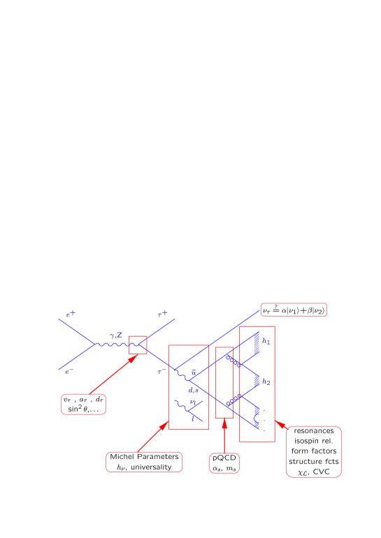
Figure 1: Selected physics topics which can be studied in $\tau$-lepton production and decay.

Recent higher-order calculations of the interdependence between the strange quark mass and the decay rate into Cabibbo suppressed channels are another important topic of Sect.3. Predictions for exclusive decays will be covered in Sect.4. This includes the technique of structure functions, predictions for form factors based on chiral dynamics, the inclusion of resonances, and constraints from CVC and isospin relations. Tau decays in combination with isospin have been used to measure the pion form factor which in turn is an important ingredient for the calculation of the anomalous magnetic moment of the muon and the electromagnetic coupling at the scale $M_{Z}$. The validity of this approach and its limitations will also be addressed in Sect.4. A selection from the many speculations on physics beyond the Standard Model will be presented in Sect.5. This includes tests for CP violation and a few new suggestions for lepton number violating decays.

The properties of the tau neutrino, in particular its mass and mixing, have received considerable attention after the observation of mixing in atmospheric neutrino studies. This topical subject will be discussed in a different section of this meeting and is therefore not included in the present review.

2 Weak Couplings

2.1 Charged Current Interactions

2.1.1 Lepton Universality in Tau Decays

Universality of weak interactions is one of the cornerstones of the present theoretical framework. Deviations could arise from additional gauge interactions which are sensitive to lepton species, thus providing a clue to the origin of the triplicate nature of the fermion spectrum, one of the mysteries of the present theory. Alternatively one might attribute a deviation from universality to mass dependent interactions, mediated for example by Higgs exchange in fairly straightforward extensions of the Standard Model.

The different tests of universality as discussed below are sensitive to different new phenomena. They should therefore be pursued as important measurements in their own right, and not simply be judged and compared on the basis of one ”figure of merit”.

i) $\tau\to\nu\pi$

The classical test of lepton universality dating back to the “pre-tau-era” is based on the comparison between the decay rates of the pion into electron and muon respectively. In lowest order this ratio is simply given by the electron and muon masses, a simple first year’s textbook calculation. A precise prediction must include radiative corrections (Fig.2) due to virtual photon exchange and real emission

$$R_{e/\mu}=\frac{\Gamma(\pi\to e\nu)}{\Gamma(\pi\to\mu\nu)}$$

$$=\frac{m_{e}^{2}}{m_{\mu}^{2}}\left(\frac{m_{\pi}^{2}-m_{e}^{2}}{m_{\pi}^{2}-m_{\mu}^{2}}\right)^{2}\left(1+\delta R_{e/\mu}\right).$$ (1)

      + + …

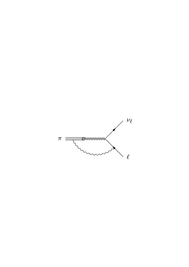
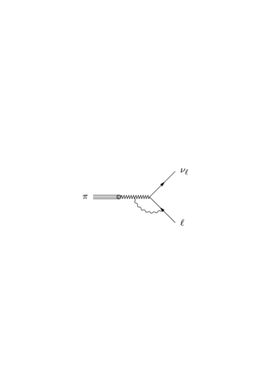
+ real emission

Figure 2: Radiative corrections affecting the pion decay.

Short distance corrections cancel in $R_{e/\mu}$ since it is the same effective Hamiltonian which governs both numerator and dominator. The dominant $m_{\ell}$ dependent correction,

$$R_{e/\mu}=\frac{3\alpha}{\pi}\ln\frac{m_{e}}{m_{\mu}}+...=-3.72\%$$ (2)

comes remarkably close to a more refined prediction including renormalization group improvement plus an estimate of the dominant logarithms from hadronic effects [1]

$$\delta R_{e/\mu}=-(3.76\pm 0.04)\%.$$ (3)

A more refined treatment [2] including a detailed modeling of hadronic form factors leads to

$$\delta R_{e/\mu}=-(3.74\pm 0.01)\%,$$ (4)

well consistent with the earlier result. The reduced theoretical uncertainty can again be traced to the long distance aspect of hadronic interactions.

The final prediction and the measurement are well consistent:

$$R^{\rm theory}_{e/\mu}=(1.2356\pm 0.0001)\cdot 10^{-4},$$ (5)

$$R^{\rm exp}_{e/\mu}=(1.230\pm 0.004)\cdot 10^{-4}.$$ (6)

Universality in this reaction is thus verified at a level of $3\cdot 10^{-3}$ and further progress is possible by improving the experimental precision.

The small uncertainty of the theoretical prediction is a natural consequence of the low momenta probed in this calculation, with $m_{\pi}$ far below $m_{\rho}$, the typical scale relevant for hadronic form factors. The situation is drastically different for tau decays. In lowest order the ratio

$$R_{\tau/\pi}=\frac{\Gamma(\tau\to\pi\nu)}{\Gamma(\pi\to\mu\nu)}$$

$$=\frac{m_{\tau}^{3}}{2m_{\pi}m_{\mu}^{2}}\left(\frac{1-m_{\pi}^{2}/m_{\tau}^{2}}{1-m_{\mu}^{2}/m_{\pi}^{2}}\right)^{2}\left(1+\delta R_{\tau/\pi}\right)$$ (7)

is again fixed by the masses of the leptons and the pion. The radiative corrections collected in $\delta R_{\tau/\pi}$ can again be predicted in leading logarithmic approximation [3]

$$1+\delta R_{\tau/\pi}=\frac{1+2\frac{\alpha}{\pi}\ln m_{Z}/m_{\tau}}{1+\frac{3}{2}\frac{\alpha}{\pi}\ln m_{Z}/m_{\pi}+\frac{1}{2}\frac{\alpha}{\pi}\ln m_{Z}/m_{\rho}}.$$ (8)

The short distance piece as given by the $\ln m_{Z}$ terms cancels again in the ratio, the remainder depends critically on the guess for the low energy cutoff. The choice as given in Eq.(8) leads to

$$\delta R_{\tau/\pi}=-0.96\%$$ (9)

with an uncertainty estimated in [3] to be $\pm 0.5\%$. A detailed explicit calculation based on a careful separation between long and short distance contributions predicts [2]

$$\delta R_{\tau/\pi}=\left(0.16^{~{}~{}+0.09}_{~{}~{}-0.14}\right)\%$$ (10)

The difference between these two results is entirely due to the more detailed treatment of long distance phenomena. The important lesson to be drawn from this comparison is that estimates of long distance effects for exclusive channels may well fail at the level of $1\%$. This uncertainty of around $1\%$ might also set the scale for predictions of $\Gamma(\tau\to\pi^{-}\pi^{0}\nu)$ based on CVC and isospin symmetry.

The prediction for decays into $\pi$ and similarly into $K$ is well consistent with the experimental result

$$B_{\pi+K}=(11.79\pm 0.12)\%.$$ (11)

The lifetime $\tau_{\tau}=290.8\pm 0.6~{}{\rm fs}$ which has to be used in this comparison as additional input is derived from the direct measurement $\tau_{\tau}=290.5\pm 1.0~{}{\rm fs}$ and the indirect result of $291.0\pm 0.7~{}{\rm fs}$ which is obtained from the leptonic branching ratios $B_{e}=17.81\pm 0.06$% and $B_{\mu}=17.36\pm 0.06$%. The test of universality, ${\rm Exp/Th}=1.013\pm 0.010$, is thus only a factor three less precise than the universality test in pion decay.

It is interesting to see that experiments with their accuracy of one percent are already able to discriminate between the theoretical predictions Eq.(9) and Eq.(10). The former, based on leading logarithm considerations only, disagrees by more than two standard deviations, the latter is consistent with the measurements. Future, improved measurements of $\tau\to\nu\pi$ will therefore be critical tests of our understanding of radiative corrections, with important implications for the validity of isospin symmetry and CVC in the prediction of $\tau\to\nu\pi^{-}\pi^{0}$ from $e^{+}e^{-}$ data discussed below (Sect. 4).

Although the present result for the mode $\tau\to\nu K$ with a branching ratio $0.71\pm 0.05$% is not yet competitive it should be emphasized that this channel is particularly interesting. It connects quarks and leptons of the second and third generation, respectively. It is particularly sensitive to exotic mass dependent effects such as charged Higgs exchange and its rate is predicted with an accuracy better than one percent.

ii)  Leptonic decays

The rates of two of the three purely leptonic decays can be calculated without theoretical ambiguity if the third one has been measured. Conventionally one chooses the muon decay rate for normalization. The electromagnetic corrections are finite and given separately in the implicit definition of $G_{F}$

$$\Gamma_{\mu}=\frac{G_{F}^{2}m_{\mu}^{5}}{192\pi^{3}}\left(1+\frac{3m_{\mu}^{2}}{5m_{W}^{2}}\right)f(\frac{m_{\mu}^{2}}{m_{W}^{2}})\left(1+\delta_{\rm QED}\right),$$

$$f(x)=1-8x+8x^{3}-x^{4}-12x^{2}\ln x$$ (12)

$$\delta_{\rm QED}=\left(\frac{\alpha\left(m_{\mu}\right)}{\pi}\right)\left(\frac{25}{8}-\frac{\pi^{2}}{2}\right)+\left(\frac{\alpha}{\pi}\right)^{2}6.743.$$

The ${\cal O}(\alpha)$ term in $\delta_{QED}$ has been calculated nearly forty years ago [4], the second term of order $\alpha^{2}$ was evaluated only recently [5].

Two independent tests of universality are thus accessible: the comparison of electronic and muonic decay rates of the $\tau$, and the comparison between one of the tau decay rates and $\Gamma_{\mu}$.

Electron-muon universality is best tested in the ratio $B_{\mu}/B_{e}$. The experimental result, expressed in terms of the ratio of couplings [6]

$$\frac{g_{\mu}}{g_{e}}=1.0015\pm 0.0025.$$ (13)

comes close in precision to the one achieved in pion decay $(1.0023\pm 0.0016)$. Higgs exchange amplitudes could in particular be enhanced in $\tau\to\mu\nu\nu$ and thus lead to observable differences in $B_{e}/B_{\mu}$ (Fig.3). In pion decays they would be practically absent.

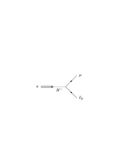
Figure 3: Amplitudes mediated by Higgs exchange.

The relative reduction of the rate in the two Higgs doublet model $-2m_{\mu}^{2}({\rm tan}\beta/m_{H})^{2}$ leads to an interesting limit on $m_{H}/{\rm tan}\beta$ in the range around or above $1$ GeV [7, 8], nearly comparable in strength to those from $b\to s\gamma$, $B\to\tau\nu$, and $Z\to b\bar{b}$. Additionally, even stronger limits have been deduced from the decay spectra, the Michel parameters, to be discussed below.

The ratio $B_{\mu}/B_{e}$ thus leads to a test of electron-muon universality. The comparison between the leptonic decay rate of the tau and the muon is in contrast sensitive to new physics phenomena connected specifically with the tau lepton. One example [9] is based on enhanced Higgs boson induced vertex corrections, which leads to a relative reduction of the rate

$$\frac{\delta\Gamma}{\Gamma}=\frac{G_{F}m_{\tau}^{2}}{16\pi^{2}}\;2\sqrt{2}\;{\rm tan}^{2}\beta\;{\cal F}\left(m_{H_{i}},\alpha_{\rm mix}\right),$$ (14)

where ${\rm tan}\beta$ is given by the ratio of the two vacuum expectation values and $\alpha_{\rm mix}$ parameterizes the mixing in the Higgs sector. Depending on the precise values of these parameters the reduction of the rate might reach a few per mille. This is indicated in Fig.4 for the specific choice $m_{H_{1}}=m_{H_{2}}=m_{H_{3}}=m_{H}$ labeling the curves, ${\rm tan}\beta=70$, and the charged Higgs mass varying between $50$ and $1000$ GeV.

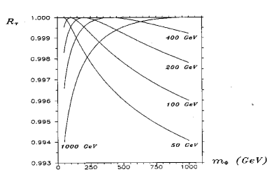
Figure 4: The ratio $1+\delta\Gamma/\Gamma$ versus the mass of the charged Higgs boson for $m_{H_{1}}=m_{H_{2}}=m_{H_{4}}=$ $40-400$ GeV and ${\rm tan}\beta=70$ [9].

Larger mass splittings typically lead to larger deviations. Present experiments with their sensitivity of a few permille [6]

$$\frac{g_{\tau}}{g_{\mu}}=1.0001\pm 0.0026$$ (15)

start to approach this interesting region.

2.1.2 Lepton Spectra, Michel Parameters, and Neutrino Helicity

i) Leptonic decays

Much of the techniques of measuring and analyzing the lepton spectrum in tau decays has been derived from the corresponding muon decay experiments. Starting from the local four fermion interaction

$${\cal M}=\frac{4G_{F}}{\sqrt{2}}\sum g_{i}\left(\bar{l}_{\rm L,R}\Gamma^{N}\nu_{l}\right)\left(\bar{\nu}_{\tau}\Gamma_{N}\tau_{\rm L,R}\right)$$ (16)

and exploiting either the “natural” polarization of $\tau$’s from $Z$ decays or the “induced” polarization from $\tau^{+}\tau^{-}$ decay correlations the four parameters $\rho,\eta,\xi$ and $\delta$ are determined consistent with the expectations from V-A interaction $3/4$, $0$, $1$ and $3/4$. The parameter $\eta$ in particular is sensitive to righthanded couplings; its measurement can be used to set interesting bounds on amplitudes induced through charged Higgs exchange [7, 8] quite comparable to those derived from the rate.

Recently the local ansatz Eq.(16) has been questioned, and a generalization including momentum dependent vertices has been introduced [10]. Starting from a coupling of the form

$${\cal A}=\frac{g}{\sqrt{2}}\bar{\tau}\left[\gamma_{\mu}+\frac{i}{2m_{\tau}}\sigma_{\mu\nu}Q^{\nu}\left(\kappa-i\tilde{\kappa}\gamma_{5}\right)\right]\nu_{\rm L}W^{\mu}$$ (17)

with $Q=P_{\tau}-P_{\nu}$ , one obtains modifications of the distributions in leptonic and semileptonic decays which are not covered by the Michel parameters. A limit on the anomalous coupling $\kappa$ obtained this way is easily converted into a limit on the compositeness scale $\Lambda=m_{\tau}/\kappa$, and experiments are getting close to interesting bounds in the range $\Lambda\sim 100$ GeV. This topic is closely related to the discussion of nonlocal neutral current interactions in Sect.2B.

ii) Semileptonic decays and neutrino helicity

Semileptonic decays offer two distinctly different methods to determine the relative magnitude of vector vs. axial amplitude in the $\tau\nu W$ coupling. Given a nonvanishing tau polarisation, the angular distribution of hadrons relative to the direction of the polarization is a direct measure of

$$h_{\nu}=\frac{2g_{V}g_{A}}{g_{v}^{2}+g_{A}^{2}},$$ (18)

with $h_{\nu}=-1$ in the V-A theory. For the pion decay for example one obtains, for example:

$$dN=\frac{1}{2}\left(1-h_{\nu}\cos\theta\right){\rm d}cos\theta.$$ (19)

For more complicated multi-meson final states the coefficient accompanying $h_{\nu}$ is smaller than one, if the hadronic final state is summed. Full analyzing power is recovered by looking into suitable angular distributions as discussed below. An alternative determination [11] of $h_{\nu}$, applicable in particular for unpolarized taus, is provided by decays into three (or more) mesons. In this case one can discriminate between hadronic states with helicity $-1$, zero or $+1$ and thus infer the neutrino helicity from the analysis of parity violating (!) angular distributions of the mesons (Fig.5).

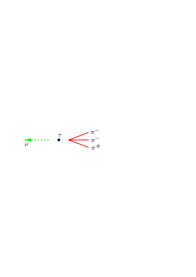
Figure 5: Three pion mode as a tool for
the measurement of the neutrino helicity.

As mentioned above, the analyzing power of two- or three-meson states in a spin one configuration is reduced by a factor $(m_{\tau}^{2}-2Q^{2})/(m_{\tau}^{2}+2Q^{2})$ which is typically around $0.5$ for two pions ($Q^{2}\approx m_{\rho}^{2}$) and close to zero for three pions $Q^{2}\approx m_{a_{1}}^{2}$. Full analyzing power of one, equal to the single pion decay, is recovered if the information on all meson momenta is retained. Starting from the decay amplitude

$${\cal M}=\frac{G_{F}}{\sqrt{2}}\bar{u}(\nu)\gamma^{\alpha}(1-\gamma_{5})u(\tau)J_{\alpha}$$ (20)

with $J_{\alpha}=\langle{\rm had}|V-A|0\rangle$ one obtains

$${\rm d}\Gamma=\frac{G_{F}^{2}}{2m}\left(\omega-{\bf H}{\bf S}\right){\rm d}PS.$$ (21)

For the single pion decay ${\bf H}/\omega=h_{\nu}{\bf n}_{\pi}$. In general ${\bf H}$ and $\omega$ are constructed from a bilinear combination of the hadronic current dependent on all meson momenta. As shown in [11, 12]

$$|{\bf H}/\omega|=1.$$ (22)

This observation is also one of the important ingredients of the Monte Carlo program TAUOLA [13], which is currently used to simulate tau decays. It has furthermore been used [14] for a simplified analysis of the tau polarization in terms of one “optimal variable”. The complete kinematic information is not immediately available in these events since the momenta of the two neutrinos from the decay of $\tau^{+}$ and $\tau^{-}$ respectively are not determined and one is left with a twofold ambiguity, even in double hadronic events. This leads to a reduction of the analyzing power for two and three meson decays. However, as shown in [15] the measurement of the tracks close to the production point with vertex detectors allows to resolve the ambiguity. Specifically, it is the direction of the vector ${\bf d}_{\rm min}$ which characterizes the distance between the tracks of $\pi^{+}$ and $\pi^{-}$ and which provides the missing piece of information for events where both taus decay into one pion each. The situation for more complicated modes is discussed in [16]

Only recently, with significant advance in the vertex detectors this technique has been applied, providing a factor two improvement compared to the result without reconstruction of the full kinematics [17].

2.2 Neutral Current Couplings

$Z$ decays into tau pairs provide an extremely powerful tool for the analysis of neutral current couplings. This has been made possible by the large event rates collected by the four LEP detectors and the inclusion of most of the tau decay modes in the analysis. At present these measurements compete with those from the SLD experiment based on longitudinally polarized beams, thus providing an important test of lepton universality in the neutral current sector and an accurate independent determination of the weak mixing angle. A first important test is obtained from a comparison of the rate [18]

$$R_{e}=20.757\pm 0.056;$$

$$R_{\mu}=20.783\pm 0.037;$$

$$R_{\tau}=20.823\pm 0.056,$$ (23)

which confirms lepton universality of neutral currents at a level comparable to the charged current result.

The $\tau$ polarization as function of the production angle $\theta$ depends on both electron and tau couplings:

$$P_{\tau}(\cos\theta)=-\frac{A_{\tau}(1+\cos^{2}\theta)+2A_{e}\cos\theta}{(1+\cos^{2}\theta)+2A_{\tau}A_{e}\cos\theta}$$ (24)

and the asymmetry coefficients

$$A_{l}=\frac{2(1-4\sin^{2}\theta_{W})}{1+(1-4\sin^{2}\theta_{W})}$$ (25)

are extremely sensitive to the effective weak mixing angle $\sin^{2}\theta_{W}$:

$$\delta A_{l}\approx 8\delta\sin^{2}\theta_{W}.$$ (26)

Table 1: Preliminary $A_{e}$ and $A_{\tau}$ results from ALEPH Collaboration with statistical and systematic uncertainties for the $1990-1995$ data based on the $\tau$ direction method. From [19].

Channel	$A_{\tau}(\%)$	$A_{e}(\%)$
hadron	$15.49\pm 1.01\pm 0.66$	$17.36\pm 1.35\pm 0.13$
rho	$13.71\pm 0.79\pm 0.57$	$15.04\pm 1.06\pm 0.078$
$a_{1}(3h)$	$15.01\pm 1.55\pm 1.30$	$15.78\pm 2.07\pm 0.40$
$a_{1}(h2\pi^{0})$	$15.94\pm 1.73\pm 1.7$	$12.65\pm 2.31\pm 0.41$
electron	$14.98\pm 2.18\pm 0,82$	$16.96\pm 2.92\pm 0.15$
muon	$14.45\pm 2.13\pm 1.06$	$12.05\pm 2.78\pm 0.24$
acol.	$13.34\pm 3.83\pm 1.8$	$19.41\pm 5.02\pm 0.24$
combi.	$14.61\pm 0.53\pm 0.37$	$15.52\pm 0.71\pm 0.09$

Table 2: Summary on $A_{\tau}$ and $A_{e}$ measurements at LEP. The first error is statistical and the second is systematic (from Ref. [19]).

Exp.	$A_{\tau}(\%)$	$A_{e}(\%)$
ALEPH	$14.52\pm 0.55\pm 0.27$	$15.05\pm 0.69\pm 0.10$
DELPHI	$13.81\pm 0.79\pm 0.67$	$13.53\pm 1.16\pm 0.33$
L3	$14.76\pm 0.88\pm 0.62$	$16.78\pm 1.27\pm 0.30$
$OPAL$	$13.4\pm 0.9\pm 1$	$12.9\pm 1.4\pm 0.5$

The conceptually simplest method to determine $P_{\tau}$ is based on the decay rate into a single pion Eq.(19). However, despite their large event rates the LEP experiments are still limited by the statistical error. Therefore it is important to use the maximum number of decay channels and exploit the full multidimensional distribution of the two [20, 11, 21] and three [11, 22, 14] pion decay mode. The importance of exploiting as many channels as possible becomes evident from Table 1, the improvement from combining the four LEP experiments is shown in Table 2. On the one had this result can be used for a test of universality:

$$\frac{A_{e}}{A_{\tau}}=1.03\pm 0.07,$$ (27)

on the other hand $A_{e}$ and $A_{\tau}$ can be combined to

$$A_{l}=(14.52\pm 0.34)\%.$$ (28)

Converted to a measurement of the effective weak mixing angle

$$\sin^{2}\theta_{W}=0.23176\pm 0.00043,$$ (29)

the result competes well with the measurement of SLD with longitudinally polarized beams [23]

$$\sin^{2}\theta_{W}=0.23110\pm 0.00029,$$ (30)

and is evidently an important ingredient in the combined LEP and SLD Standard Model fit which gives [24]

$$\sin^{2}\theta_{W}=0.23155\pm 0.00019.$$ (31)

The result from $\tau$ polarization alone is about a factor five more accurate than anticipated in the original plans for physics at LEP where an accuracy $\delta\sin^{2}\theta_{W}\leq 0.002$ was considered a reasonable goal [25].

2.3 Electric and Magnetic Dipole Moments

As a member of the third family with a mass drastically larger than the one of the electron or muon the tau lepton is ideally suited for speculations about anomalous couplings to the photon as well as the $Z$ boson. The effects of the electric or anomalous magnetic moments or their weak analogues increase with the energy, hence $Z$ decays are particularly suited for these investigations. Constraints on the weak couplings are derived from the decay rate or from $CP$ violating correlations in the decay $Z\to\tau^{+}\tau^{-}$ [26]. By searching for an excess of hard noncollinear photons in the radiative final state $\tau^{+}\tau^{-}\gamma$ of the $Z$ boson decays give also access to anomalous electromagnetic couplings.

Table 3: Limits on the electromagnetic and weak dipole moments of $\tau$ (from Ref. [27])

	$\gamma\tau\bar{\tau}$	$Z\tau\bar{\tau}$
$a_{\tau}$	$-0.05<a_{\tau}<0.06$	$\begin{array}[]{l}\Re=(0.0\pm 1.6\pm 2.3)10^{-3}\\ \Im=(-1.0\pm 3.6\pm 4.3)10^{-3}\end{array}$
$\begin{array}[]{c}d_{\tau}\\ \!\!\![10^{-16}\mbox{e~{}cm}]\!\!\!\end{array}$	$-3<d_{\tau}<3$	$|d_{\tau}|\leq 0.1$

Table 4: Limits on anomalous dipole moments of electron and muon.

	$e$	$\mu$
$|a-a_{Th}|\,[\mu_{B}]$	$\leq 10^{-11}$	$\leq 10^{-8}$
$d[e\,\mbox{cm}]$	$(0.18\pm 0.16)10^{-26}$	$(3.7\pm 3.4)10^{-19}$

The present experimental limits as listed in Table 3 are by many orders of magnitude less restrictive than these from low energy precision measurements of Table 4.

However, general considerations suggest dramatic enhancement of anomalous couplings with the lepton mass; at least proportional to $m_{l}^{2}$, eventually even $m_{l}^{4}$. In particular in the latter case studies of the tau lepton could open the window to completely novel phenomena.

3 Inclusive Decays, Perturbative QCD, and Sum Rules

3.1 Inclusive Decays and the Strong Coupling Constant

The total $\tau$ decay rate into hadrons has become one of the key elements in the measurements of the strong coupling constants. The ratio $R_{\tau}$ can be expressed in terms of $\Pi^{[1]}$ and $\Pi^{[2]}$ which arise from the tensorial decomposition of the correlator of the V-A current

$$R_{\tau}=\frac{\Gamma(\tau\to\nu+{\rm hadrons})}{\Gamma(\tau\to e\nu\bar{\nu})}=6\pi i\int\limits_{|s|=m_{\tau}^{2}}\frac{{\rm d}s}{m_{\tau}^{2}}$$

$$\times\left(1-s/m_{\tau}\right)^{2}\left[\Pi^{[2]}(s)-\frac{2}{m_{\tau}^{2}}\Pi^{[1]}(s)\right]$$ (32)

with

$$i\int{\rm d}xe^{iqx}\langle 0|T[j_{\mu}^{V-A}(x)j_{\nu}^{V-A}(0)]|0\rangle=$$

$$g_{\mu\nu}\Pi^{[1]}+q_{\mu}q_{\nu}\Pi^{[2]}.$$ (33)

The contour integral receives contributions from the region of (relatively) large $|s|\sim m_{\tau}^{2}$ only, and $\Pi^{[1]}$ as well as $\Pi^{[2]}$ can be calculated in perturbative QCD. Their absorptive parts are available up to order $\alpha^{3}_{s}$. As a consequence of the present ignorance of $c_{4}$, the coefficient of the $\alpha^{4}_{s}$ term, and the large value of $\alpha_{s}$ at the scale $m_{\tau}$ different – at present equivalent – prescriptions for the evaluation lead to significantly different results for $\alpha_{s}$ at $m_{\tau}$ and correspondingly at $M_{z}$ [28]. Once ”educated guesses” for $c_{4}$, based on dominant terms in the perturbative series are implemented, the spread in $\alpha_{s}$ decreases significantly [29].

Recent measurements (see eg. [30, 28] and references therein) of the differential rate ${\rm d}\Gamma/{\rm d}s$ where $s$ denotes the mass of the hadronic system have led to a large number of consistency tests, strengthening the confidence in this precision measurement of $\alpha_{s}$. Moments $R_{\tau}^{kl}$ are defined by introducing additional weight functions $(1-s/m_{\tau}^{2})^{k}(s/m_{\tau})^{l}$ which can be measured [28, 30] and at the same time calculated in pQCD [31].

The separation of vector and axial contributions to the spectral function is fairly simple for final states with pions, $\eta$ and $\eta\prime$ only and thus of well-defined $G$ parity. However, additional theoretical input is needed for the $K\bar{K}\pi$ channel which has contributions from both $J^{P}=1^{+}$ and $1^{-}$. In fact, recent experimental results [32] seem to confirm theoretical predictions [33, 34] of axial dominance.

The analysis of moments of $R_{\tau}^{V}(s)$ and $R_{\tau}^{A}(s)$ separately leads to an improved determination of the vacuum condensates [30, 28], the weighted integrals of the difference

$$I_{i}(s_{0})=\frac{1}{4\pi^{2}}\int\limits_{s_{m}in}^{s_{0}}{\rm d}sf_{i}(s)\left(R_{V}(s)-R_{A}(s)\right)$$ (34)

are particularly sensitive to nonperturbative aspects. Experimental results are shown in Fig.6 for four choices, corresponding to four different sum rules

$$f_{1}(s)=1\Rightarrow$$

$$I_{1}=f_{\pi}^{2}~{}\left({\rm first~{}Weinberg}\right)$$ (35)

$$f_{1}(s)=s\Rightarrow$$

$$I_{2}=0~{}\left({\rm second~{}Weinberg}\right)$$ (36)

$$f_{3}(s)=\frac{1}{s}\Rightarrow$$

$$I_{3}=f_{\pi}^{2}\frac{r_{\pi}^{2}}{3}-F_{A},~{}\left({\rm Das,Matur,Okubo}\right)$$ (37)

$$f_{4}(s)=s\ln\frac{s}{\lambda^{2}}\Rightarrow$$

$$I_{4}=-\frac{4\pi}{3\alpha}f_{\pi}^{2}\left(m_{\pi^{+}}^{2}-m_{\pi^{0}}^{2}\right)$$ (38)

and compared to the respective theoretical prediction.

Figure 6: Experimental results for four different sum rules, Eqs.(35-38). (From [28], see also [30])

The evolution of $a=\alpha_{s}/\pi$ from the low scale $m_{\tau}$ up to $M_{Z}$ is essential for any meaningful comparison of results obtained at vastly different energies. Three ingredients are crucial for any renormalization group analysis, the $\beta$ function

$$\frac{{\rm d}\ln a}{{\rm d}\ln\mu^{2}}=-a\left(\beta_{0}+\beta_{1}a+\beta_{2}a^{2}+\beta_{3}a^{3}\right)$$ (39)

the anomalous mass dimension $\gamma$

$$\frac{{\rm d}\ln\bar{m}}{{\rm d}\ln\mu^{2}}=-a\left(\gamma_{0}+\gamma_{1}a+\gamma_{2}a^{2}+\gamma_{3}a^{3}\right)$$ (40)

and the relation between the couplings $a_{n}$ and $a_{n+1}$ which are valid for the theories with n and n+1 effective quark species respectively

$$a_{n+1}(m_{n+1}^{2})=a_{n}(m_{n+1}^{2})\left(1+c_{2}a^{2}+c_{3}a^{3}\right).$$ (41)

Important progress has been achieved during the past two years in the calculation of all three relations: the four-loop term of the $\beta$ function $\beta_{3}$ has been evaluated with considerable effort and heavy machinery of algebraic programs [35], similarly the corresponding four-loop term $\gamma_{3}$ of the anomalous mass dimension [36] and, last not least, the coefficient $c_{3}$ of the matching relation [37]. Fig.7 demonstrates as a characteristic example the dependence of $\alpha_{s}^{(5)}(M_{Z})$ on the choice of the matching point $\mu^{5}$ for the transition between QCD with four and five flavors respectively. Phenomenological studies, based on [35, 36, 37] can also be found in [38].

Figure 7: $\mu^{(5)}$ dependence of $\alpha_{s}^{(5)}(M_{z})$ calculated from $\alpha_{s}^{(4)}(m_{\tau})=0.36$ and $m_{b}=4.7$ GeV using decoupling relations at one (dotted), two (dashed), three (dot-dashed) and four (solid) loop (from [37]).

3.2 Cabibbo Suppressed Decays and the Strange Quark Mass

Tau decays into final states with strangeness proceed at the fundamental level through the transition of the virtual $W$ to $s$ plus $\bar{u}$ quarks and are thus affected by the relatively large strange quark mass. After separating off the suppression through the mixing angle $\sin^{2}\theta_{C}$ the remaining reduction of the rate in comparison to the light quark $d$ plus $\bar{u}$ configuration can be attributed to strange quark mass $m_{s}$. Two important consequences are related to $m_{s}\neq 0$: the divergence of both vector and axial correlator is different from zero:

$$q_{\mu}q_{\nu}\Pi^{VA}_{\mu\nu}=m_{s}^{2}\Pi^{S,P}+m_{s}\left(\langle\bar{s}s\rangle\pm\langle\bar{u}u\rangle\right),$$ (42)

where $\Pi^{S,P}$ is related to the scalar correlator, which is available [39] in order $\alpha^{3}_{s}$ up to the constant term. Eq.(42) leads in particular to the production of final states with spin zero and $q^{2}\neq 0$. However, also the rate for the $J=1$ configuration, or of suitably chosen moments of the spectral function are significantly affected. The correlator for vector and axial currents

$$g_{\mu\nu}\Pi^{[1]}+q_{\mu}q_{\nu}\Pi^{[2]}.$$ (43)

can always be expanded in $m_{s}^{2}/q^{2}$ and the subsequent discussion is restricted to the leading quadratic mass term. The perturbative results can thus be cast in the following form:

$$\Pi^{[1]}={\rm massless~{}result}+\frac{3}{8\pi^{2}}m_{s}^{2}\left[l_{q}+a(...)+\right.$$

$$\left.a^{2}(...)+a^{3}\left(l_{q}^{4}+...+l_{q}+k_{3}^{(1)}\right)\right],$$ (44)

$$\Pi^{[2]}={\rm massless~{}result}-\frac{3m_{s}^{2}}{4\pi^{2}q^{2}}\left[1+a(...)+\right.$$

$$\left.a^{2}(...)+a^{3}\left(l_{q}^{3}+...+l_{q}+k_{3}^{(2)}\right)\right]$$ (45)

with $a=\alpha_{s}/\pi$ and $l_{q}=\ln q^{2}/\mu^{2}$. The constants $k_{3}^{[1,2]}$ are presently unknown. While $k_{3}^{[1]}$ is irrelevant for the evaluation of the quadratic mass terms in the integral Eq.(32), the constant $k_{3}^{[2]}$ contributes to the result, a consequence of the additional factor $1/q^{2}$. Higher moments, with their additional factor $s$ in the integrand can be calculated in fixed order pQCD consistently up to order $\alpha^{3}_{s}$.

As stated above, the two independent quantities $\Pi^{[1]}$ and $\Pi^{[2]}$ which enter the integral for $R_{\tau}$ carry independent information in the case $m_{s}\neq 0$. It is therefore of interest to separately consider spin zero and spin one contributions to $R_{\tau}$. To obtain the spin zero part $R^{J=0}_{\tau}$ one has to replace the expression in $\Pi^{[2]}-2\Pi^{[1]}/m_{\tau}^{2}$ by $\Pi^{(0)}(s)-\Pi^{[1]}(0)/s$. The first term $\Pi^{(0)}$ vanishes in the limit $m_{s}\to 0$ within perturbation theory, in the second term the factor $\Pi^{[1]}(0)$ is clearly a nonperturbative object which for the $d\bar{u}$ final states describes the pion contribution. This term disappears for moments with $l\geq 1$. Moments of $R^{J=0}_{\tau}$ with $l\geq 1$ are thus a direct measure of the strange quark mass.

It is therefore of interest to calculate the $m_{s}$ dependence of the rate [40, 41], of moments of the spectral function [42, 43], and furthermore of the corresponding quantities for the spin separated objects [43].

$$\delta^{kl}=b_{0}\frac{m_{s}^{2}(m_{\tau})}{m_{\tau}^{2}}\left(1+b_{1}a+b_{2}a^{2}+b_{3}a^{3}\right)=$$

$$\hat{b}_{0}\frac{m_{s}^{2}(1{\rm GeV})}{m_{\tau}^{2}}\left(1+\hat{b}_{1}a+...\right),~{}~{}~{}k,l\geq 0$$ (46)

The second choice of the scale has also been tried [43] in order to slightly reduce the surprisingly large coefficients. However, the reduction is only marginal and the subsequent discussion will be for $\mu=m_{\tau}$ only. For the total rate one finds

$$\delta^{00}=-8\frac{m_{s}^{2}}{m_{\tau}^{2}}\left(1+5.33a+46a^{2}+248a^{3}+\right.$$

$$\left.+248a^{3}+0.75k_{3}^{[2]}a^{3}\right)$$

$$=-8\frac{m_{s}^{2}}{m_{\tau}^{2}}\left(1+0.567+0.520+0.341\pm 0.148\right)$$

$$=-8\frac{m_{s}^{2}}{m_{\tau}^{2}}\left(2.4\pm 0.5\right)$$ (47)

where $a=\alpha_{s}/\pi=0.106$ has been adopted. The error estimate is based on the assumption of geometric growth of the coefficients $k^{[2]}_{i}$ in Eq.(45). A slight improvement of the “convergence” is observed for the so-called contour improved prediction, which has been studied for the massless case in [44, 31, 45]. In this case the integral along the large circle in the complex plane with $|s|=m_{\tau}^{2}$ is evaluated numerically, with $\alpha_{s}(s)$ calculated numerically from the renormalization group with the $\beta$ function up to the four-loop coefficient. In this case one finds

$$\delta^{00}=-8\frac{m_{s}^{2}}{m_{\tau}^{2}}\left(1.44+0.389+0.349+\right.$$

$$\left.0.0867\pm 0.234\right)=-8\frac{m_{s}^{2}}{m_{\tau}^{2}}\left(2.26\pm 0.32\right)$$ (48)

The strong growth of the series can be traced to the longitudinal piece of the correlator. The apparent convergence is more promising in the case of the spin one part alone. For the lowest moment that can be evaluated in perturbation theory one finds, for example

$$\delta^{01}|_{J=1}=-5\frac{m_{s}^{2}}{m_{\tau}^{2}}\left(1.37+0.271+0.182+0.163\right)$$

$$=-5\frac{m_{s}^{2}}{m_{\tau}^{2}}\left(2.0\pm 0.2\right).$$ (49)

Coefficients of the higher moments with and without spin separation, can be found in [43].

At the time of this workshop, the experimental analysis has been performed for the total rate only [46, 47]. The (unimportant) $m_{s}$ dependent terms of dimension $4$ and $6$ are available in order $\alpha^{2}_{s}$ and $\alpha_{s}$ respectively. Applying these new theoretical results to the experimental analysis of [46, 47] one obtains the result

$$m_{s}(1{\rm GeV})=\left(200\pm 40_{\rm exp}\pm 30_{\rm th}\right)~{}~{}{\rm MeV},$$ (50)

which is in fair agreement with different, independent evaluations. The theoretical error estimate should be considered for the moment as a rough guess only. First steps towards the separation of $J=0$ and $J=1$ as well as the analysis of moments can be found in [48].

4 Exclusive Decays

4.1 Form Factors and Structure Functions

The determination of form factors in exclusive decays is not only required for a precise test of theoretical predictions. The separation of vector and axial–vector amplitudes and their respective spin zero and one contributions is mandatory for a number of improved phenomenological studies like the determination of $\alpha_{s}$ and nonperturbative vacuum condensates based on moments of vector and axial spectral functions separately, or the unambiguous separation of vector contributions (in particular in the $KK\pi$ channels) for $\alpha_{QED}(M_{Z})$. Just like the search for CP violation (discussed below) or the measurement of $g_{V}^{\tau}/g_{A}^{\tau}$ through parity violation in hadronic decays, this can be performed with the help of a combined analysis of angular and energy distributions of the hadrons, even without reconstruction of the $\tau$-restframe.

In the three (two) meson case, the most general ansatz for the hadronic matrix element of the quark current, $J^{\mu}(q_{1},q_{2}(,q_{3}))\equiv\langle h_{1}(q_{1})h_{2}(q_{2})(h_{3}(q_{3}))|V^{\mu}(0)-A^{\mu}(0)|0\rangle$, is characterized by four (two) complex form factors $F_{i}$, which are in general functions of $s_{ij}\equiv(q_{i}+q_{j})^{2}$ and $Q^{2}$ ($Q^{\mu}\equiv\sum_{i}q_{i}^{\mu}$):

$$J^{\mu}(q_{1},q_{2})\!\!\!=\!\!\!T^{\mu\nu}\,(q_{1}-q_{2})_{\nu}\,F+Q^{\mu}\,F_{S}\,,$$ (51)

$$J^{\mu}(q_{1},q_{2},q_{3})\!\!\!=\!\!\!T^{\mu\nu}\left[\,(q_{1}-q_{3})_{\nu}\,F_{1}\,+\right.$$

$$\left.\,(q_{2}-q_{3})_{\nu}\,F_{2}\,\right]+\,\,i\,\epsilon^{\mu\alpha\beta\gamma}q_{1\,\alpha}q_{2\,\beta}q_{3\,\gamma}\,F_{3}+$$

$$Q^{\mu}\,F_{4}\,.$$

$T^{\mu\nu}=g^{\mu\nu}-(Q^{\mu}Q^{\nu})/Q^{2}$ denotes a transverse projector. The form factors $F_{1}$ and $F_{2}$ originate from the $J^{P}=1^{+}$ axial–vector hadronic current, and $F_{3}$ ($F$) from the $J^{P}=1^{-}$ vector current; they correspond to a hadronic system in a spin one state, whereas $F_{4}$ ($F_{S}$) are due to the $J=0$ part of the axial–vector (vector) current matrix element. These form factors contain the full dynamics of the hadronic decay. For a two–pion final state, $h_{1}h_{2}=\pi^{-}\pi^{0}$, $F_{S}\equiv 0$ in the isospin symmetry limit ($m_{u}=m_{d}$). In the three pion case, $h_{1}h_{2}h_{3}=\pi^{-}\pi^{-}\pi^{+}$ or $\pi^{0}\pi^{0}\pi^{-}$, Bose symmetry implies $F_{2}(Q^{2},s_{23},s_{13})=F_{1}(Q^{2},s_{13},s_{23})$; $G$–parity conservation requires $F_{3}\equiv 0$ for $m_{u}=m_{d}$, and $F_{4}$ vanishes when $m_{u}=m_{d}=0$.

In experimental analyses, the four(two) complex form factors in Eq.(51) appear as sixteen (four) real “structure” functions $W_{X}$, which are defined from hadronic tensor $H^{\mu\nu}=J^{\mu}J^{\nu}$ in the hadronic rest frame [22]. The contributions of the different $F_{i}$ to $W_{X}$ are summarized in Table 5. After integration over the unobserved neutrino direction, the differential decay rate in the hadronic rest frame is given in the two-meson case by [22, 49]

$${\rm d}\Gamma(\tau^{-}\to 2h\nu_{\tau})=\{\bar{L}_{B}W_{B}+\bar{L}_{SA}W_{SA}+$$

$$\bar{L}_{SF}W_{SF}+\bar{L}_{SG}W_{SG}\}$$

$$\times\frac{G_{F}^{2}}{2m_{\tau}}\sin^{2}\theta_{c}\frac{1}{(4\pi)^{3}}\frac{(m_{\tau}^{2}-Q^{2})^{2}}{m_{\tau}^{2}}|{\bf q_{1}}|\frac{{\rm d}Q^{2}}{\sqrt{Q^{2}}}$$

$$\times\frac{{\rm d}\cos\theta}{2}\frac{{\rm d}\alpha}{2\pi}\frac{{\rm d}\cos\beta}{2}.$$ (52)

The functions $\bar{L}_{X}$ depend on the angles and energies of the hadrons only [22, 49]. The hadronic structure function $W_{X}$ in the two meson case depend only on $Q^{2}$ and the form factors $F$ and $F_{S}$ of the hadronic current. Similarly, the differential decay rate in the three meson case is given by [22]:

$${\rm d}\Gamma=\frac{G_{F}^{2}}{4m_{\tau}}\left(\begin{array}[]{c}\cos\theta_{c}^{2}\\ \sin\theta_{c}^{2}\end{array}\right)\sum\limits_{X}\bar{L}_{X}W_{X}{\rm d}PS^{(4)}.$$ (53)

The sum in Eq.(53) runs (in general) over $16$ hadronic structure functions $W_{X}$, which correspond to $16$ density matrix elements for a hadronic system in a spin one and spin zero state (nine of them originate from a pure spin one state and the remaining originate from a pure spin zero state or from interference terms between spin zero and spin one, see Table 5). These structure functions contain the dynamics of the hadronic decay and depend only on the form factors $F_{i}$. Note that $W_{A}$, $W_{B}$ and $W_{SA}$ alone determine ${\rm d}\Gamma/{\rm d}Q^{2}$ through

$$\frac{{\rm d}\Gamma(\tau\to h_{1}h_{2}h_{3}\nu_{\tau})}{{\rm d}Q^{2}}\propto\frac{(m_{\tau}^{2}-Q^{2})^{2}}{Q^{4}}$$

$$\times\int{\rm d}s_{1}{\rm d}s_{2}\left\{(1+\frac{Q^{2}}{m_{\tau}^{2}})\frac{W_{A}+W_{B}}{6}+\frac{W_{SA}}{2}\right\}.$$

(Almost) all structure functions can be determined by studying angular distributions of the hadronic system, for details see [22]. This method allows to analyze separately the contribution from $J^{P}=0^{+},0^{-},1^{+}$ and $1^{-}$ in a model independent way (see Table 5.)

In the differential decay distribution, the four (two) complex form factors appear as sixteen (four) real “structure functions” $W_{X}$, which are defined from the hadronic tensor $H^{\mu\nu}=J^{\mu}J^{\nu*}$ in the hadronic rest frame [22]. For the precise definitions of $W_{X}$, we refer the reader to Ref. [22]. The contributions of the different $F_{i}$ to $W_{X}$ are summarized in Table 5. Almost all structure functions can be determined by studying angular distributions of the hadronic system, which allows to analyze separately the contributions from $J^{P}=0^{+},0^{-},1^{+}$ and $1^{-}$ in a model–independent way.

Table 5: Structure functions for exclusive $\tau$ decays

$$\begin{array}[]{|c|c|c|c|}\hline\cr&\vrule\lx@intercol\hfil H^{\mu}\longrightarrow\hfil\lx@intercol\vrule\lx@intercol\\ H^{\nu*}\downarrow&J^{P}=1^{+}&J^{P}=1^{-}&J=0\\ \hline\cr\\[-8.53581pt] J^{P}=1^{+}&{\bf W_{A}}&&\\ &W_{C}W_{D}W_{E}&&\\ \hline\cr\\[-8.53581pt] J^{P}=1^{-}&W_{F}W_{G}&{\bf W_{B}}&\\ &W_{H}W_{I}&&\\ \hline\cr\\[-8.53581pt] J=0&W_{SB}W_{SC}&W_{SF}W_{SG}&{\bf W_{SA}}\\ &W_{SD}W_{SG}&&\\ \hline\cr\hline\cr\\[-17.07164pt] &&\vrule\lx@intercol\hfil\underbrace{\hskip 64.58313pt}_{\displaystyle h_{1}h_{2}}\hfil\lx@intercol\vrule\lx@intercol\\ \hline\cr\\[-17.07164pt] &\vrule\lx@intercol\hfil\underbrace{\hskip 129.16626pt}_{\displaystyle h_{1}h_{2}h_{3}}\hfil\lx@intercol\vrule\lx@intercol\\ \hline\cr\end{array}$$

4.2 Chiral Dynamics

Chiral Lagrangians allow for a prediction of the formfactors in the limit of small momenta. This approach is particularly useful for final states with a low number, say up to three or four pions, which can still be treated as massless Goldstone bosons [50].

In lowest order of Chiral Perturbation Theory (CPT) the formfactors are constants and the polynomial dependence of the amplitude is essentially fixed by the Lorentz structure of the amplitude which in turn is imposed by the quantum numbers of the currents and the charge and multiplicity of the pions. The same approach is also applicable for final states with kaons or $\eta$ mesons, although their treatment as massless Goldstone bosons and the assumption of small momenta becomes more dubious in these cases.

Figure 8: Differential decay rate for $\tau\to 2\pi\nu_{\tau}$: Predictions by CHPT at $O(p^{2})$ (dashed), at $O(p^{4})$ (dashed-dotted), at $O(p^{6})$ (solid), and from a vector meson dominance model (dotted), compared with exp. data from CLEO (dots with error bars) (from Ref. [51]).

The validity of CPT can be extended to larger momentum transfer by including one and even two-loop corrections [51]. For the pion formfactor shown in Fig.8 one observes a stronger upward curvature –similar to the expectation from vector dominance, where the lowest order chiral amplitude is simply augmented by the $\rho$ meson propagator $M^{2}/(M^{2}-Q^{2}-i\Gamma M)$ or its more refined variants with the proper $Q^{2}$ dependent width.

A more elaborated approach along the same lines has been presented recently [52, 53], which tries to combine CPT, constraints from analyticity and VDM to arrive at an improved description of the data over a wide energy range. The amplitudes, describing the decay to $\nu_{\tau}$ plus three pions ($\pi^{-}\pi^{-}\pi^{+}$ or $\pi^{-}\pi^{0}\pi^{0}$) have been calculated in CPT in Born approximation [50]and including one loop corrections [51]. The lowest order prediction , even including $a_{1}$ and $\rho$ mesons through vector dominance, leads to identical predictions for both charge configurations. Inclusion of chiral loops, however, leads to a remarkable differences between the amplitude for the two cases, which is in particular reflected in a difference even of the sign of the structure function $w_{D}$ for small momenta [51].

4.3 Resonances

The kinematical region of soft mesons, in particular pions, is accessible to the rigorous approach of CPT. The major fraction of final states is, however, concentrated at intermediate momenta, a region dominated by a multitude of resonances. For two pions the amplitude is well described by $\rho$ (plus $\rho^{\prime}$, etc.) dominance, with one out of many successful parameterizations given for example in [54]. In this type of model the normalization of the amplitude is deduced from the low energy limit, the structure of the amplitude from the masses and widths of the resonances. The generalization of this approach for the three pion case [50, 54, 55] describes successfully angular distributions, energy spectra and distributions in the Dalitz plot, which are conventionally encoded in the structure functions (see e.g. Ref.[56]).

Final states with strangeness lead to significantly more involved substructure of the resonances. The pseudoscalar resonance in the configuration $\bar{K}^{0}\pi^{-}\pi^{0}$ can have subresonances in the $(\bar{K}^{0}\pi^{-})=\bar{K}^{*-}$, in the $(\bar{K}^{0}\pi^{0})=\bar{K}^{*0}$ or the $\pi^{-}\pi^{0}=\rho^{-}$ system. With $G$ parity being irrelevant in this mode, both vector and axial vector current contribute, which allows for a nonvanishing formfactor $F_{4}$ (see Eq.(51)). Furthermore, with $m_{s}\neq 0$, the currents are no longer conserved, which allows for a small $J^{P}=0^{-}$ amplitude $F_{3}\neq 0$. The formfactors are again conveniently calculated in the chiral limit, the predicted total rate and the mass distributions depend crucially on the parameters of the resonances, their masses and widths which are often poorly determined and must be treated as free parameters. A typical example can be found in [33, 34]. In these papers it is shown that the branching ratio for the decay into $K^{-}\pi^{-}\pi^{+}$ decreases from the originally predicted [57] $0.77\%$ to $0.45\%$ if both the widths of $K_{1}(1400)$ and $K_{1}(1270)$ are increased from the PDG values of $174$ MeV and $90$ MeV respectively to $250$ MeV. This lower result is in acceptable agreement with the current world average [58] of $0.304\pm 0.074$, in particular since no refined fit of the input parameters on the basis of differential distributions has been performed.

4.4 Isospin and CVC

Important constraints on relations among amplitudes and decay rates into seemingly different channels can be derived using isospin symmetry (or, to lesser extent $SU(3)$ symmetry). In addition, one may use isospin and the hypothesis of a conserved vector current (CVC) to relate rates for hadrons produced in $\tau$ decays and in electron positron annihilation. The technique of partitions and symmetry classes, originally developed for proton-antiproton annihilation at low energies [59] has been extensively applied to $\tau$ decays [60, 61, 21]. The two partial rates into four pions $\Gamma(--+0)$ and $\Gamma(-000)$ are determined by the two channels for electron-positron annihilation into four pions and vice versa, for six pions on the other hand only upper and lower limits can be derived. By the same kind of reasoning also final states with kaons can be interrelated. For example [62]

$$\Gamma(K^{-}\pi^{+}\pi^{-}) = \frac{1}{2}\Gamma(\bar{K}^{0}\pi^{-}\pi^{0})+2\Gamma(k^{-}\pi^{0}\pi^{0})$$

$$2\Gamma(K^{0}K^{-}\pi^{0}) \leq \Gamma(K^{0}\bar{K}^{0}\pi^{-})=\Gamma(K^{+}K^{-}\pi^{-}),$$

nicely consistent with recent experimental results [32].

Up to this point only relations among decay rates have been considered. In addition one may, in some cases, also exploit relations among amplitudes for different charge conjugations. Defining, for example, for the three pion state

$$\langle pi_{1}^{0}\pi_{2}^{0}\pi^{-}|J^{\mu}|0\rangle=J^{\mu}(p_{1},p_{2},p^{-})+J^{\mu}(p_{2},p_{1},p^{-}),$$ (54)

one predicts

$$\langle\pi_{1}^{-}\pi_{2}^{-}\pi^{+}|J^{\mu}|0\rangle=J^{\mu}(p^{+},p_{1},p_{2})+$$ (55)

$$J^{\mu}(p^{+},p_{2},p_{1})+J^{\mu}(p_{1},p^{+},p_{2})+J^{\mu}(p_{2},p^{+},p_{1}).$$

Only in the special case that the function $J$ is antisymmetric with respect to the second and third variable the predictions for the amplitude of $(0,0,-)$ and $-,-,+$ configurations coincide. In general, however, differences are possible, in particular if there is a marked resonance in the isospin zero configuration.

Similarly, one obtains relations between amplitude of the four-pion final states. Given

$$\langle\pi^{+}\pi^{-}\pi_{1}^{0}\pi_{2}^{0}|J^{\mu}|0\rangle=J^{\mu}(p^{+},p^{-},p_{1},p_{2})$$ (56)

one predicts for $e^{+}e^{-}\to 4\pi$

$$\langle\pi^{+}\pi^{+}\pi^{-}\pi^{-}|J^{\mu}|0\rangle=J^{\mu}(p_{1}^{+},p_{1}^{-},p_{2}^{+},p_{2}^{-})+$$

$$J^{\mu}(p_{2}^{+},p_{1}^{-},p_{1}^{+},p_{2}^{-})+J^{\mu}(p_{1}^{+},p_{2}^{-},p_{2}^{+},p_{1}^{-})+$$

$$J^{\mu}(p_{2}^{+},p_{2}^{-},p_{1}^{+},p_{1}^{-})$$ (57)

and for $\tau\to 4\pi\nu$

$$\langle\pi^{-}\pi^{0}\pi^{0}\pi^{0}|J^{\mu}|0\rangle=J^{\mu}(p^{-},p_{1},p_{2},p_{3})+$$

$$J^{\mu}(p^{-},p_{2},p_{1},p_{3})+J^{\mu}(p^{-},p_{3},p_{1},p_{2})$$

$$\langle\pi^{-}\pi^{-}\pi^{+}\pi^{0}|J^{\mu}|0\rangle=J^{\mu}(p_{1},p^{0},p^{+},p_{2})+$$

$$J^{\mu}(p_{2},p^{0},p^{+},p_{2})$$

which connects at the same time $\tau$ decays and electron positron annihilation.

Analogous results are derived for final states with kaons. Given the amplitude for the transitions to $\pi^{-}\pi^{0}\bar{K}^{0}$ and $\pi^{0}\pi^{0}K^{-}$

$$\langle\pi^{-}\pi^{0}\bar{K}^{0}|J_{\mu}|0\rangle=J_{\mu}^{I=1}(q_{-},q_{0},q_{K}),$$ (58)

$$\langle\pi^{0}\pi^{0}K^{-}|J_{\mu}|0\rangle=J_{\mu}^{I=0}(q_{1},q_{2},q_{K}),$$ (59)

which leads necessarily to the two pions in the $I=1$ and $I=0$ configurations. The amplitudes are odd under $q_{-}\leftrightarrow q_{0}$ (even under $q_{1}\leftrightarrow q_{2}$) and one obtains:

$$\langle\pi^{+}\pi^{-}\bar{K}^{-}|J_{\mu}|0\rangle=$$ (60)

$$J_{\mu}^{I=0}(q_{+},q_{-},q_{K})-\frac{1}{\sqrt{2}}J_{\mu}^{I=1}(q_{+},q_{-},q_{K}).$$

4.5 Hadronic Vacuum Polarization from $\tau$ Decays

The hadronic vacuum polarization is of central importance for the evaluation and interpretation of various precision observables. This applies in particular to the fine structure constant at high energies and the anomalous magnetic moment of the muon. Both are strongly influenced by low energy contributions to the famous $R$ ratio. In the low energy region, it is dominated by the two pion state, with its amplitude given by pion form factor.

Originally, the decay $\tau\to\nu\pi^{-}\pi^{0}$ was predicted from the pion form factor as measured in electron positron annihilation. However, with the excellent normalization in $\tau$ decays, $\delta\Gamma/\Gamma(\tau\to\nu\pi^{-}\pi^{0})=6\cdot 10^{-3}$, significant improvement could be obtained and the experimental error of the analysis of $a_{\mu}$ [63] is largely dominated by $\tau$ data

$$a_{\mu}|_{\pi^{+}\pi^{-}}10^{10}=\left\{\begin{array}[]{cc}495.86\pm 12.46&e^{+}e^{-}\\ 500.81\pm 6.03&{\rm incl.}\tau\end{array}\right.$$ (61)

However, the transformation from $\tau$ to $e^{+}e^{-}$ data

$$\frac{{\rm d}\Gamma(\tau\to\nu\pi^{-}\pi^{0})}{{\rm d}s}\propto S_{ew}\sigma(e^{+}e^{-}\to\pi^{+}\pi^{-})$$ (62)

is subject to some theoretical uncertainties which have to be scrutinized. The short distance electroweak corrections, collected in

$$S_{ew}=1.0194\approx 1+\frac{\alpha}{\pi}\ln\frac{M_{Z}^{2}}{m_{\tau}^{2}}$$ (63)

are derived from the inclusive rate. Large distance corrections are not included and could be channel dependent. For the cutoff scale, a number of choices, for example $m_{\tau},m_{\rho}$ or $m_{\pi}$ are available.

The theoretical uncertainty has been estimated in [3] around $0.5\%$. However, already the difference between the qualitative evaluation of $\Gamma(\tau\to\nu\pi^{-})$ in [3] and the detailed investigation in [2] amounts to $1.1\%$. This could well be considered as a realistic estimate of theoretical uncertainties from long distance correction effects as long as radiative corrections are based on inclusive rates only. (New preliminary from CMD-2 experiment in Novosibirsk [64] indicate a deviation of more than $3\%$. These large differences would prevent the use of the $\tau$ data for precision measurements of the form factor.) In addition there is the problem of separating the vector and axial contributions in the $K\bar{K}\pi$ channel in $\tau$ decays which can be solved, at least in principle, by using the technique of structure functions described in Sect.4.1. At this point it may be worthwhile to emphasize an important difference between the hadronic contributions to $a_{\mu}$ and $\alpha(M_{Z})$. The former is largely dominated by very low energy data, the latter receives contributions from the full energy region up to $M_{Z}$, with a weight $dQ^{2}/Q^{2}$. This has prompted theory driven analyses [65, 66, 67, 68, 69] which employ the $\tau$ and $e^{+}e^{-}$ data at low energies, perturbative QCD for energies above $1.8$ GeV and away from the charm and bottom thresholds. An important ingredient in this analysis are theoretical results for the $R$ ratio in order $\alpha_{s}^{2}$ and $\alpha_{s}^{3}$ including quark mass effects [70, 71, 72].

The relative size of various contributions to $\Delta\alpha(M_{Z})|_{\rm had}$ is listed in Table 6, a compilation of recent results on $\Delta\alpha(M_{z})|_{\rm had}$ from different authors is shown in Table 7.

Table 6: Contributions to $\Delta\alpha^{(5)}_{\rm had}(M_{Z}^{2})$ from different energy regions. From Ref. [66].

Input	energy region	$\Delta\alpha^{(5)}\times 10^{4}$
low energy data [65]	$2m_{\pi}-1.8$ GeV	$56.90\pm 1.10$
narrow charmonium resonances	$J/\Psi,\Psi(2S),\Psi(3770)$	$9.24\pm 0.74$
“normalized” data	$3.7-5.0$ GeV	$15.67\pm 0.34$
$\Upsilon$ resonances	$\Upsilon(1S)-\Upsilon(11.019)$	$1.17\pm 0.09$
interpolation of $b\bar{b}$	$11.075-11.2$	$0.03\pm 0.03$
pQCD (and QED)	$1.8-\infty$	$194.45\pm 0.96$
	total	$277.45\pm 1.68$

Although $\tau$ data and pQCD have lead to significant improvements, independent confirmation from electron positron colliders is highly desirable. The low energy region, being of prime importance for the muon anomalous magnetic moment, will be exploited by VEPP-2M and DAPHNE, intermediate energies up to $5$ GeV at BES2. Improved measurement at CESR or the $B$-factories could further strengthen our confidence in pQCD at the relatively high energy of $10$ GeV.

The $\phi$-factory DAPHNE and the $B$-factories plan to operate primarily at their designed energy around $1$ GeV and $10$ GeV. Using radiative events with tagged photon, one could well explore a large energy region, with $\sqrt{Q^{2}}$ varying from the two pion threshold up to $\sqrt{s}$.

The differential cross section

$$s\frac{{\rm d}\sigma}{{\rm d}Q^{2}{\rm d}\cos\theta}=\frac{\alpha}{2\pi}\sigma(Q^{2})\frac{1}{1-\cos^{2}\theta_{\gamma}}$$

$$\times\left((1+\cos^{2}\theta_{\gamma})\underbrace{\frac{(s-Q^{2})}{s}}_{\sim 1}+\underbrace{\frac{4Q^{2}}{s-Q^{2}}}_{\ll 1}\right)$$ (64)

is proportional to $\sigma(Q^{2})$, the cross section for the $e^{+}e^{-}$ annihilation into corresponding hadronic state at lower energies. The factor $1/(1-\cos^{2}\theta_{\gamma})$ leads to predominance of initial state radiation versus final state radiation for small photon angles. The $Q^{2}$ dependence of the last factor is fairly flat in the region $Q^{2}\ll s$. Since $\sigma(Q^{2})$ is integrated with a flat weight (again for $Q^{2}\ll M_{z}^{2}$)

$$\Delta\alpha_{\rm had}(M_{z}^{2})\sim\int{\rm d}Q^{2}\sigma(Q^{2})\left[\frac{M_{z}^{2}}{(M_{z}^{2}-Q^{2})}\right]$$ (65)

the photon energy resolution is not necessary crucial for the analysis. The detailed analysis, based on a Monte Carlo generator [73] demonstrates that initial and final state radiation can be reasonably well separated, if proper cuts on pion and photon angles are imposed.

Table 7: Comparison of different evaluations of $\Delta\alpha^{(5)}_{\rm had}(M_{Z}^{2})$. (${}^{*}\Delta\alpha_{\rm top}(M_{Z}^{2})$ subtracted.) From Re.[66]

$\Delta\alpha^{(5)}_{\rm had}(M_{Z}^{2})\times 10^{4}$	Reference
$273.2\pm 4.2$	[74], Martin et al. ‘95
$280\pm 7$	[75], Eidelman et al. ‘95
$280\pm 7$	[76], Burkhardt et al. ‘95
$275.2\pm 4.6$	[77], Swartz ‘96
$281.7\pm 6.2$	[78], Alemany et al. ‘97
$278.4\pm 2.6^{*}$	[65], Davier et al. ‘97
$277.5\pm 1.7$	[66], Kühn et al. ‘98

5 Beyond the Standard Model

5.1 CP Violation in Hadronic $\tau$ Decays

CP violation has been experimentally observed only in the $K$ meson system. The effect can be explained by a nontrivial complex phase in the CKM flavour mixing matrix. However, the fundamental origin of CP violation is still unknown. In particular the CP properties of the third fermion family are largely unexplored. Production and decay of $\tau$ leptons might offer a particularly clean laboratory to study these effects. CP violation which could arise in a framework outside the conventional mechanism could be observed [16] in semileptonic $\tau$ decays. The structure function formalism Sect.4.1 allows for a systematic analysis of possible CP violation effects in the two and three meson channels. Special emphasize is put on the $\Delta S=1$ transitions $\tau\to K\pi\nu_{\tau}$, where possible CP violating signals from multi Higgs boson models would be signaled by a nonvanishing difference between the structure function $W_{SF}(\tau^{-}\to(K\pi)^{-}\nu_{\tau})$ and its charge conjugate. Such a measurement is possible for unpolarized single $\tau$’s without reconstruction of the $\tau$ rest frame and without polarized incident $e^{+}e^{-}$ beams. This CP violation requires both non-vanishing hadronic phases and $CP$ violating phases in the Hamiltonian. The hadronic phases arise from the interference of complex Breit-Wigner propagators, whereas the CP violating phases could arise from an exotic charged Higgs boson. An additional independent test of CP violation in the two meson case is possible, but would require the knowledge of the full kinematics and $\tau$ polarization (or correlation studies).

Transitions from the vacuum to pseudoscalar mesons $h_{1}$ and $h_{2}$ are induced through vector current and scalar currents only. The general amplitude for the $\Delta S=1$ decay (where $h_{1}=K$ and $h_{2}=\pi$)

$$\tau^{-}(l,s)\to nu(l^{\prime},s^{\prime})+h_{1}(q_{1},m_{1})+h_{2}(q_{2},m_{2}),$$ (66)

thus can be written as

$${\cal M}=\sin\theta_{c}\frac{G_{F}}{\sqrt{2}}\bar{u}(l^{\prime},s^{\prime})\gamma_{\alpha}(1-\gamma_{5})u(l,s)$$

$$\times\left[(q_{1}-q_{2})_{\beta}T^{\alpha\beta}F+Q^{\alpha}\hat{F}_{S}\right]$$ (67)

with

$$\hat{F}_{S}=F_{S}+\frac{\eta_{S}}{m_{\tau}}F_{H}.$$ (68)

In Eq.(67) $s$ denotes the polarization four-vector of the $\tau$ lepton. The complex parameter $\eta_{S}$ in Eq.(68) transforms like

$$\eta_{S}\to\eta_{S}^{*}$$ (69)

and thus allows for the parameterization of possible $CP$ violation.

$W_{SF}$ can be measured in $e^{+}e^{-}$ annihilation experiments through the study of single unpolarized $\tau$ decays, even if the $\tau$ rest frame cannot be reconstructed [16]. This differs from earlier studies where either polarized beams and reconstruction of the full kinematics [79] or correlated fully reconstructed $\tau^{-}$ and $\tau^{+}$ decays were required [80]. The determination of $W_{SG}$, however, requires the knowledge of the full $\tau$ kinematics and $\tau$ polarization [16] (eventually to be substituted through correlation studies) which is possible with the help of vertex detectors. The corresponding distributions in this latter case are similar to the correlations proposed in [79, 80].

The crucial observation is that one can measure the following CP-violating differences:

$$\Delta W_{SF} = \frac{1}{2}\left(W_{SF}[\tau^{-}]-W_{SF}[\tau^{+}]\right),$$

$$\Delta W_{SG} = \frac{1}{2}\left(W_{SG}[\tau^{-}]-W_{SG}[\tau^{+}]\right).$$ (70)

One obtains

$$\Delta W_{SF}=4\sqrt{Q^{2}}|{\bf q}_{1}|\frac{1}{m_{\tau}}{\rm Im}(FF_{H}^{*}){\rm Im}[\eta_{S}].$$ (71)

In essence the measurement of $\Delta W_{SF}$ analyses the difference in the correlated energy distribution of the mesons $h_{1}$ and $h_{2}$ from $\tau^{+}$ and $\tau^{-}$ decay in the laboratory. A nonvanishing $\Delta W_{SF}$ requires nontrivial hadronic phases (in addition to CP violating phases $\eta_{S}$) in the form factors $F$ and $F_{H}$. Such hadronic phases in $F(F_{H})$ originate in the $K\pi\nu_{\tau}$ decay mode from complex Breit-Wigner propagators for the $K^{*}(K_{0}^{*})$ resonance.

Once the $\tau$ rest frame is known and a preferred direction of polarization exists (eventually through the use of correlations between $\tau^{+}$ and $\tau^{-}$ decays) one may also determine

$$\Delta W_{SG}=4\sqrt{Q^{2}}|{\bf q}_{1}|\frac{1}{m_{\tau}}{\rm Re}(FF_{H}^{*}){\rm Im}[\eta_{S}].$$ (72)

The sensitivity to CP violating effects in $\Delta W_{SF}$ and $\Delta W_{SG}$ can be fairly different depending on the hadronic phases. First steps have been undertaken by the CLEO collaboration to perform an experimental analysis along these lines [81].

The structure function formalism [22] allows also for a systematic analysis of possible CP–violation effects in the three meson case [82]. The $K\pi\pi$ and $KK\pi$ decay modes with nonvanishing vector and axial–vector current are of particular importance for the detection of possible CP violation originating from exotic intermediate vector bosons. This would be signaled by a nonvanishing difference between the structure functions $W_{X}(\tau^{-})$ and $W_{X}(\tau^{+})$ with $X\in\,\{F,G,H,I\}$. A difference in the structure functions with $X\in\,\{SB,SC,SD,SE,SF,SG\}$ can again be induced through a CP violating scalar exchange. CP violation in the three pion channel has been also discussed in [83] and in the $K\pi\pi$ and $KK\pi$ channels in [84], where the latter analysis is based on the “$T-$odd” correlations in [22] and the vector–meson–dominance parameterizations in [85].

5.2 “Forbidden” Decays

A large variety of decay modes which are strictly forbidden in the Standard Model with massless neutrinos has been searched experimentally. They could violate lepton family number, lepton number or baryon number, and upper limits of a few $10^{-6}$ have been reached [86].

Heavy Dirac or Majorana type neutrinos, natural ingredients in Grand Unified Theories, would in fact induce the corresponding “Dirac type” ($\tau^{-}\to l^{-}+...$) or “Majorana type ” ($\tau^{-}\to l^{+}+...$) decays through virtual corrections. The detailed theoretical analysis performed for final states with one-meson [87] and two-mesons [88] channels show that branching ratios around $10^{-6}$ are reasonable targets for a dedicated search program.

6 Acknowledgments

Many thanks to Toni Pich and Alberto Ruitz for an enjoyable and productive workshop. This paper would have never been completed without the TeXnical help of K. Melnikov.

I benefited greatly from instructive discussions with K. Chetyrkin, M. Davier, A. Hoecker, C. Geweniger, A. Pivovarov, A. Stahl, M. Steinhauser and N. Wermes on various theoretical and experimental aspects of $\tau$ physics.

References

- [1] W.J. Marciano and A. Sirlin, Phys. Rev. Lett. 71 (1993) 3629.
- [2] R. Decker and M. Finkemeier, Nucl. Phys. B438 (1995) 17.
- [3] W.J. Marciano and A. Sirlin, Phys. Rev. Lett. 61 (1988) 1815.
- [4] T. Kinoshita and A. Sirlin, Phys. Rev. 113 (1959), 1652; S.H. Berman, Phys. Rev. 112 (1958) 267.
- [5] T. van Ritbergen and R.G. Stuart, hep-ph/9808283.
- [6] G. Passaleva, talk presented at ICHEP 98, Vancouver, July 1998.
- [7] A. Stahl and H. Voss, Zeit. f. Phys. C74 (1997) 73.
- [8] A. Stahl, these proceedings.
- [9] R.J. Guth, A.H. Hoang and J.H. Kühn, Phys. Lett. B285 (1992) 75.
- [10] M.T. Dova, T. Swain, L. Taylor, hep-ph/9712384.
- [11] J.H. Kühn and F. Wagner, Nucl. Phys. B136 (1984) 16.
- [12] J.H. Kühn, Phys. Rev. D52 (1995) 3128.
- [13] S. Jadach, J.H. Kühn and Z. Was, Comp. Phys. Comm. 64 (1991) 275.
- [14] M. Davier, L. Duflot, F. le Diberder and A. Rouge, Phys. Lett. B306 (1993) 411.
- [15] J.H. Kühn, Phys. Lett. B313 (1993), 458.
- [16] J.H. Kühn and E. Mirkes, Phys. Lett. B398 (1997) 407
- [17] ALEPH collaboration, Contribution to the ICHEP98, Vancouver 1998, ALEPH 98-073; M.Wunsch, these proceedings.
- [18] The LEP Collaborations, the LEP Electroweak Working Group and the SLD Heavy Flavour Group, CERN-PPE 97-154.
- [19] R. Alemany, these proceedings.
- [20] P. Tsai, Phys. Rev. D4 (1971) (1971), 28.
- [21] A. Rouge, Workshop on Tau Lepton Physics, Orsay 1990, Edition Frontiers (1991) pg. 213.
- [22] J.H. Kühn and E. Mirkes, Zeit. f. Physik C56 (1992), 661; erratum ibid. C67 (1995), 364; Phys. Lett. B286 (1992), 281.
- [23] K. Baird, presented at ICHEP 98, Vancouver, July 1998.
- [24] D. Karlen, presented at ICHEP 98, Vancouver, July 1998.
- [25] G. Altarelly, in Physics at LEP, CERN86-02.
-
[26]
H. Wermes, Nucl. Phys. B55C
(Proc. Suppl.) (1997) 313 and references therein;
J. Vidal et al., these proceedings. - [27] P. Garcia-Abia, talk presented at ICHEP-98, Vancover 1998; see also A. Zalite, these proceedings; T. Barklow, these proceedings.
- [28] S. Menke, these proceedings
- [29] C.J. Maxwell, these proceedings.
- [30] A. Hoecker, these proceedings
- [31] F. Le Diberder and A. Pich, Phys. Lett. B286 (1992) 147.
- [32] S. Chen, these proceedings.
- [33] M. Finkemeier, J.H. Kühn and E. Mirkes, Nucl. Phys. 55C (Proc. Suppl.) (1997) 169.
- [34] J.H. Kühn, E. Mirkes and J. Willibald, Proc. Int. Conf. on High Energy Physics, Jerusalem, Israel, 1997, hep-ph/9712263.
- [35] S.A. Larin, T. van Ritbergen and J. Vermaseren, Phys. Lett. B400 (1997), 379.
-
[36]
K.G. Chetyrkin, Phys. Lett. B404 (1997), 161;
J. A. M. Vermaseren, T. van Ritbergen and S.A. Larin, Phys. Lett. B405 (1997) 327. - [37] K.G. Chetyrkin, B.A. Kniehl and M. Steinhauser, Phys. Rev. Lett. 79 (1997) 2184; Nucl. Phys. B510 (1998) 61.
- [38] G. Rodrigo, A. Pich and A. Santamaria, Phys. Lett. B424 (1998) 367.
- [39] K.G. Chetyrkin, Phys. Lett. B390 (1997) 309.
- [40] K.G. Chetyrkin and A. Kwiatkowsky, Zeit. f. Physik C59 (1993), 525.
- [41] K. Maltman, Phys. Rev. D58 (1998), 93015
- [42] J. Prades, A. Pich, Journ. of High Energy Physics 06, (1998) 13.
- [43] K.G. Chetyrkin, J.H. Kühn and A.A. Pivovarov, Nucl. Phys. B533 (1998) 473.
-
[44]
A.A. Pivovarov, Sov. J. Nucl. Phys. 54 (1991) 676;
Z. Phys. C53 (1992) 461; Nuovo Cim. 105A (1992) 813. - [45] F. Le Diberder and A. Pich, Phys. Lett. B289 (1992) 165.
- [46] M.Davier, Nucl. Phys. C55 (Proc. Suppl.) (1997) 395.
- [47] S. Chen, Nucl. Phys. C64 (Proc. Suppl.) (1998) 265.
- [48] S. Chen, M. Davier and A. Hoecker, these proceedings.
- [49] M. Finkemeier and E. Mirkes, Z. f. Phys. C72 (1996) 619.
- [50] R. Fischer, J. Wess and F. Wagner, Zeit. f. Physik C3 (1980) 313.
-
[51]
G. Colanglo, M. Finkemeier and R. Urech, Phys. Rev. D54
(1996) 4403;
G. Colangelo et al., Nucl. Phys. B (Proc. Suppl.) 55C (1997) 325. - [52] F. Guerrero and A. Pich, Phys. Lett. B412 (1997), 382.
- [53] F. Guerrero, Phys. Rev. D57 (1998), 4136.
- [54] J.H. Kühn, A. Santamaria, Zeit. f. Phys. C48 (1990) 445.
- [55] A. Pich, in SLAC report-343, pg. 416.
- [56] OPAL-Coll., K. Ackerstaff et al., Zeit. f Phys. C75 (1997) 593.
- [57] M. Finkemeier and E. Mirkes, Zeit. f. Phys. C69 (1996) 243.
- [58] B.K. Heltsey, these proceedings.
- [59] A. Pais, Ann. Phys. 9 (1960) 548, Ann. Phys. 22 (1963) 274.
- [60] F.J. Gilman and S.H. Rhie, Phys. Rev. D31 (1985) 1066.
- [61] R.J. Sobie, Zeit. f. Phys. C69 (1995) 99.
- [62] A. Rouge, Zeit. f. Phys. 70 (1996), 65; Eur. Phys. J. C4 (1998), 265.
- [63] R. Alemany, M. Davier, A. Hoecker, Eur. Phys. J. C2 (1998) 123.
- [64] S.I. Eidelman, these proceedings.
- [65] A. Hoecker and M. Davier, Phys. Lett. B419 (1998) 419.
- [66] J.H. Kühn and M. Steinhauser, Phys. Lett. B437 (1998), 425.
- [67] A. Hoecker and M. Davier, Phys. Lett. B435 (1998) 427.
- [68] J. Erler, hep-ph/9803453.
- [69] S. Groote et al., hep-ph/9802374.
- [70] K.G. Chetyrkin, J.H. Kühn, M. Steinhauser and T. Teubner, Eur. Phys. J. C2 (1998) 137.
- [71] K.G. Chetyrkin, J.H. Kühn and M. Steinhauser, Nucl. Phys. B482 (1996), 213.
- [72] A.H. Hoang, J.H. Kühn and T. Teubner, Nucl. Phys. B452 (1995), 173.
- [73] S. Alsmayer, J.H. Kühn, K. Melnikov, in preparation.
- [74] A.D. Martin and D. Zeppenfeld, Phys. Lett. B 345 (1995) 558.
- [75] S. Eidelman and F. Jegerlehner, Z. Phys. C67 (1995) 585.
- [76] H. Burkhardt and B. Pietrzyk, Phys. Lett. B 356 (1995) 389.
- [77] M.L. Swartz, Phys. Rev. D 53 (1996) 5268.
- [78] R. Alemany, M. Davier and A. Höcker, Eur. Phys. J. C 2 (1998) 123.
- [79] Y.S. Tsai, Phys. Rev. D51 (1995) 3172.
- [80] C.A. Nelson et al., Phys. Rev. D50 (1994) 4544, and references therein.
- [81] K. Erklund, these proceedings.
- [82] M. Finkemeier and E. Mirkes, Proc. Workshop on the Tau/Charm Factory (Argonne, 1995), ed. J. Repond, AIP Conf. Proc. No. 349 (New York, 1996) p. 119 [hep-ph/9508312].
- [83] S. Choi, K. Hagiwara and M. Tanabashi, Phys. Rev. D52 (1995) 1614.
- [84] U. Kilian, J. Körner, K .Schilcher and Y. Wu, Z. Phys. C62 (1994) 413.
- [85] R. Decker, E. Mirkes, R. Sauer and Z. Was, Z. Phys. C58 445 (1993).
- [86] Particle Data Group, 1998.
- [87] A. Ilakovac, B.A. Kniehl and A. Pilaftsis, Phys. Rev. D52 (1995) 3993.
- [88] A. Ilakovac, Phys. Rev. D54 (1996) 5653.