UMN-TH-1728/98

TPI-MINN-98/23

hep-ph/9811444

November 1998

GENERALIZED LIMITS TO THE NUMBER OF LIGHT PARTICLE DEGREES OF FREEDOM FROM BIG BANG NUCLEOSYNTHESIS

Keith A. Olive

University of Minnesota, School of Physics and Astronomy

Theoretical Physics Institute

116 Church St SE, Minneapolis, MN 55455

David Thomas

University of Chicago, Astronomy & Astrophysics Center

5640 S Ellis Ave, Chicago, IL 60637

Abstract

We compute the big bang nucleosynthesis limit on the number of light neutrino degrees of freedom in a model-independent likelihood analysis based on the abundances of ⁴He and ⁷Li. We use the two-dimensional likelihood functions to simultaneously constrain the baryon-to-photon ratio and the number of light neutrinos for a range of ⁴He abundances $Y_{p}$ = 0.225 – 0.250, as well as a range in primordial ⁷Li abundances from (1.6 to 4.1) $\times 10^{-10}$. For (⁷Li/H)${}_{p}=1.6\times 10^{-10}$, as can be inferred from the ⁷Li data from Population II halo stars, the upper limit to $N_{\nu}$ based on the current best estimate of the primordial ⁴He abundance of $Y_{p}=0.238$, is $N_{\nu}<4.3$ and varies from $N_{\nu}<3.3$ (at 95% C.L.) when $Y_{p}=0.225$ to $N_{\nu}<5.3$ when $Y_{p}=0.250$. If ⁷Li is depleted in these stars the upper limit to $N_{\nu}$ is relaxed. Taking (⁷Li/H)${}_{p}=4.1\times 10^{-10}$, the limit varies from $N_{\nu}<3.9$ when $Y_{p}=0.225$ to $N_{\nu}\mathrel{\mathchoice{\lower 3.6pt\vbox{\halign{$\mathsurround=0pt\displaystyle\hfil#\hfil$\cr<\crcr\sim\crcr}}}{\lower 3.6pt\vbox{\halign{$\mathsurround=0pt\textstyle\hfil#\hfil$\cr<\crcr\sim\crcr}}}{\lower 3.6pt\vbox{\halign{$\mathsurround=0pt\scriptstyle\hfil#\hfil$\cr<\crcr\sim\crcr}}}{\lower 3.6pt\vbox{\halign{$\mathsurround=0pt\scriptscriptstyle\hfil#\hfil$\cr<\crcr\sim\crcr}}}}6$ when $Y_{p}=0.250$. We also consider the consequences on the upper limit to $N_{\nu}$ if recent observations of deuterium in high-redshift quasar absorption-line systems are confirmed.

1 Introduction

One of the most important limits on particle properties is the limit on the number of light particle degrees of freedom at the the time of big bang nucleosynthesis (BBN) [1]. This is commonly computed as a limit on the number of light neutrino flavors, $N_{\nu}$. Recently, we [2] used a model-independent likelihood method (see also [3, 4]) to simultaneously constrain the value of the one true parameter in standard BBN, the baryon-to-photon ratio $\eta$, together with $N_{\nu}$. For similar approaches, see [5]. In that work [2], we based our results on the best estimate of the observationally determined abundance of ⁴He, $Y_{p}=0.234\pm 0.002\pm 0.005$ from [6], and of ⁷Li, ⁷Li/H $=(1.6\pm 0.1)\times 10^{-10}$, from [7]. While these determinations can still be considered good ones today, there is often discussion of higher abundance for ⁴He as perhaps indicated by the data of [8] and higher abundances of ⁷Li due to the effects of stellar depletion (see e.g. [9]). Rather than be forced to continually update the limit on $N_{\nu}$ as the observational situation evolves, we generalize our previous work here and compute the upper limit on $N_{\nu}$ for a wide range of possible observed abundances of ⁴He and ⁷Li. Because the determinations of D/H in quasar absorption system has not dramatically improved, we can only comment on the implications of either the high or low D/H measurements.

One of the major obstacles in testing BBN using the observed abundances of the light element isotopes rests on our ability to infer from these observations a primordial abundance. Because ⁴He, in extragalactic HII regions, and ⁷Li, in the atmospheres of old halo dwarf stars, are both measured in very low metallicity systems (down to 1/50th solar for ⁴He and 1/1000th solar for ⁷Li), very little modeling in the way of galactic chemical evolution is required to extract a primordial abundance for these isotopes. Of course systematic uncertainties, such as underlying stellar absorption, in determining the ⁴He abundance and the effects of stellar depletion of ⁷Li lead to uncertainties in the primordial abundances of these isotopes, and it is for that reason we are re-examining the limits to $N_{\nu}$. Nevertheless, the problems in extracting a primordial ⁴He and ⁷Li abundance pale in comparison with those for D and ³He, both of which are subject to considerable uncertainties not only tied to the observations, but to galactic chemical evolution. In fact, ³He also suffers from serious uncertainties concerning its fate in low mass stars [10]. ³He is both produced and destroyed in stars making the connection to BBN very difficult.

Deuterium is totally destroyed in the star formation process. As such, the present or solar abundance of D/H is highly dependent on the details of a chemical evolution model, and in particular the galactic star formation rate. Unfortunately, it is very difficult at the present time to gain insight on the primordial abundance of D/H from chemical evolution given present and solar abundances since reasonably successful models of chemical evolution can be constructed for primordial D/H values which differ by nearly an order of magnitude [11].

Of course much of the recent excitement surrounding deuterium concerns the observation of D/H in quasar absorption systems [14]-[17]. If a single value for the D/H abundance in these systems could be established, then one could avoid all of the complications concerning D/H and chemical evolution, and because of the steep monotonic dependence of D/H on $\eta$, a good measurement of D/H would alone be sufficient to determine the value of $\eta$ (since D/H is nearly independent of $N_{\nu}$). In this case, the data from ⁴He and ⁷Li would be most valuable as a consistency test on BBN and in the case of ⁴He, to set limits on particle properties. In the analysis that follows, we will discuss the consequences of the validity of either the high or low D/H determinations.

Using a likelihood analysis based on ⁴He and ⁷Li [4], a probable range for the baryon-to-photon ratio, $\eta$ was determined. The ⁴He likelihood distribution has a single peak due to the monotonic dependence of ⁴He on $\eta$. However, because the dependence on $\eta$ is relatively flat, particularly at higher values of $Y_{p}$, this peak may be very broad, yielding little information on $\eta$ alone. On the other hand, because ⁷Li is not monotonic in $\eta$, the BBN prediction has a minimum at $\eta_{10}\simeq 3$ ($\eta_{10}=10^{10}\eta$) and as a result, for an observationally determined value of ⁷Li above the minimum, the ⁷Li likelihood distribution will show two peaks. The total likelihood distribution based on ⁴He and ⁷Li is simply the product of the two individual distributions. In [4], the best fit value for $\eta_{10}$ based on the quoted observational abundances was found to be 1.8 with a 95% CL range

$$1.4<\eta_{10}<4.3$$ (1)

when restricting the analysis to the standard model, including $N_{\nu}=3$. In determining (1) systematic errors were treated as Gaussian distributed. When D/H from quasar absorption systems (those showing a high value for D/H [14, 16]) is included in the analysis this range is cut to $1.50<\eta_{10}<2.55$.

In [2], the maximum likelihood analysis of [3, 4] which utilized a likelihood function ${\cal L}(\eta)$ for fixed $N_{\nu}=3$ was generalized to allow for variability in $N_{\nu}$. There a more general likelihood function ${\cal L}(\eta,N_{\nu})$ was applied to the current best estimates of the primordial ⁴He and ⁷Li abundances. Based on the analysis in [6], we chose $\hbox{$Y_{\rm p}$}=0.234\pm 0.002\rm(stat.)\pm 0.005(syst.)$ as well as the lower value $\hbox{$Y_{\rm p}$}=0.230\pm 0.003\rm(stat.)\pm 0.005(syst.)$ based on a low metallicity subset of the data. Using these values of $Y_{\rm p}$ along with the value (Li/H)${}_{p}=(1.6\pm 0.07)\times 10^{-10}$ from [7], we found peak likelihood values $\eta_{10}=1.8$ and $N_{\nu}=3.0$ with a 95% CL range of $1.6\leq N_{\nu}\leq 4.0,1.3\leq\eta_{10}\leq 5.0$ for the higher ⁴He value and similar results for the lower one. More recent data from Izotov and Thuan [19] seems to indicate a still higher value for $Y_{\rm p}$, and for this reason as well as wishing to be independent of the “current” best estimate of the abundances, we derive our results for a wide range of possible values for $Y_{p}$ and (Li/H)_p which will account for the possibility of stellar depletion for the latter [9]. Finally, in [2], we considered only the effect of the high D/H value from quasar absorption systems. Since there was virtually no overlap between the likelihood functions based on the low D/H value and the other two elements, there was little point in using that value in our analysis. Since then, the low D/H value has been raised somewhat, and that together with our present consideration of higher $Y_{\rm p}$ and (Li/H)_p values makes the exercise worth while.

In this paper, we follow the approach of [2] – [4] in constraining the theory on the basis of the ⁴He and ⁷Li data and to a lesser extent D/H, by constructing a likelihood function ${\cal L}(\eta,N_{\nu})$. We discuss the current status of the data in section 2, and indicate what range of values for the primordial abundances we consider. In section 3, we display the likelihood functions we use. As this was discussed in more detail in [2, 4], we will be brief here. Our results are given in section 4, and we draw conclusions in section 5.

2 Observational Data

Data pertinent to the primordial ⁴He abundance is obtained from observations of extragalactic HII regions. These regions have low metallicities (as low as 1/50th solar), and thus are presumably more primitive than similar regions in our own Galaxy. The ⁴He abundance used to extract a primordial value spans roughly an order of magnitude in metallicity (e.g. O/H). Furthermore, since there have been a considerable number of such systems observed with metallicities significantly below solar, modeling plays a relatively unimportant role in obtaining the primordial abundance of ⁴He (see e.g. [20]).

The ⁴He data based on observations in [21, 8] were discussed in detail in [6]. There are over 70 such regions observed with metallicities ranging from about 2–30% of solar metallicity. This data led to the determination of a primordial ⁴He abundance of $\hbox{$Y_{\rm p}$}=0.234\pm 0.002\rm(stat.)\pm 0.005(syst.)$ used in [2]. That the statistical error is small is due to the large number of regions observed and to the fact that the ⁴He abundance in these regions is found to be very well correlated to metallicity. In fact, as can be understood from the remarks which follow, the primordial ⁴He abundance is dominated by systematic rather than statistical uncertainties.

The compilation in [6] included the data of [8]. Although this data is found to be consistent with other data on a point by point basis, taken alone, it would imply a somewhat higher primordial ⁴He abundance. Furthermore, the resulting value of $Y_{\rm p}$ depends on the method of data analysis. When only ⁴He data is used to self-consistently determine the ⁴He abundance (as opposed to using other data such as oxygen and sulphur to determine the parameters which characterize the HII region and are needed to convert an observation of a ⁴He line strength into an abundance), a value of $Y_{\rm p}$ as high as $0.244\pm 0.002$ can be found [8].

The problem concerning ⁴He has been accentuated recently with new data from Izotov and Thuan [19]. The enlarged data set from [21, 19] was considered in [20]. The new resulting value for $Y_{\rm p}$ is

$$\hbox{$Y_{\rm p}$}=0.238\pm 0.002\rm(stat.)\pm 0.005(syst.)$$ (2)

The new data taken alone gives $\hbox{$Y_{\rm p}$}=0.2444\pm 0.0015$ when using the method based on a set of 5 helium recombination lines to determine all of the H II region parameters. By more conventional methods, the same data gives $\hbox{$Y_{\rm p}$}=0.239\pm 0.002$. As one can see, the ⁴He data is clearly dominated by systematic uncertainties.

There has been considerably less variability in the ⁷Li data over the last several years. The ⁷Li abundance is determined by the observation of Li in the atmospheres of old halo dwarf stars as a function of metallicity (in practice, the Fe abundance). The abundance used in [2] from the work in [7] continues to lead to the best estimate of the ⁷Li abundance in the so called Spite plateau

$$y_{7}\equiv\frac{\hbox{${}^{7}$Li}}{\rm H}=(1.6\pm 0.07)\times 10^{-10}$$ (3)

where the error is statistical, again due to the large number of stars observed. If we employ the basic chemical evolution conclusion that metals increase linearly with time, we may infer this value to be indicative of the primordial Li abundance.

In [2], we noted that there are considerable systematic uncertainties in the plateau abundance. It is often questioned as to whether the Pop II stars have preserved their initial abundance of Li. While the detection of the more fragile isotope ⁶Li in two of these stars may argue against a strong depletion of ⁷Li [22, 9], it is difficult to exclude depletion of the order of a factor of two. Therefore it seems appropriate to allow for a wider range in ⁷Li abundances in our likelihood analysis than was done in [2].

There has been some, albeit small, change in the D/H data from quasar absorption systems. Although the re-observation of the high D/H in [23] has been withdrawn, the original measurements [14] of this object still stand at the high value. More recently, a different system at the relatively low redshift of $z=0.7$ was observed to yield a similar high value [16]

$$y_{2}\equiv{\rm D/H}=(2\pm 0.5)\times 10^{-4}.$$ (4)

The low values of D/H in other such systems reported in [15] have since been refined to show slightly higher D/H values [17]

$$y_{2}\equiv{\rm D/H}=(3.4\pm 0.3)\times 10^{-5}.$$ (5)

Though this value is still significantly lower than the high D/H value quoted above, the low value is now high enough that it contains sufficient overlap with the ranges of the other light elements considered to warrant its inclusion in our analysis.

3 Likelihood Functions

Monte Carlo and likelihood analyses have been discussed at great length in the context of BBN [24, 25, 26, 27, 28, 29, 3, 4, 2]. Since our likelihood analysis follows that of [4] and [2], we will be very brief here. The likelihood function for ⁴He, $L_{4}(N_{\nu},\eta)$ is determined from a convolution of a theory function

$$L_{\rm 4,Theory}(Y,N_{\nu},\eta)={1\over\sqrt{2\pi}\sigma_{Y}(N_{\nu},\eta)}\exp{\left({-(Y-\hbox{$Y_{\rm p}$}(N_{\nu},\eta))^{2}\over 2\sigma_{Y}^{2}(N_{\nu},\eta)}\right)}$$ (6)

(where $\hbox{$Y_{\rm p}$}(N_{\nu},\eta)$ and $\sigma_{Y}(N_{\nu},\eta)$ represent the results of the theoretical calculation) and an observational function

$$L_{\rm 4,Obs}(Y)={1\over\sqrt{2\pi}\sigma_{Y0}}\exp{\left({-(Y-Y_{0})^{2}\over 2\sigma_{Y0}^{2}}\right)}$$ (7)

where $Y_{0}$ and $\sigma_{Y0}$ characterize the observed distribution and are taken from Eqs. (2) and (3). The full likelihood function for ⁴He is then given by

$$L_{4}(N_{\nu},\eta)=\int dY\,L_{\rm 4,Theory}(Y,N_{\nu},\eta)L_{\rm 4,Obs}(Y)$$ (8)

which can be integrated (assuming Gaussian errors as we have done) to give

$$L_{4}(N_{\nu},\eta)={1\over\sqrt{2\pi(\sigma_{Y}^{2}(N_{\nu},\eta)+\sigma_{Y0}^{2})}}\exp\left({-(\hbox{$Y_{\rm p}$}(N_{\nu},\eta)-Y_{0})^{2}\over 2(\sigma_{Y}^{2}(N_{\nu},\eta)+\sigma_{Y0}^{2})}\right)$$ (9)

The likelihood functions for ⁷Li and D are constructed in a similar manner. The quantities of interest in constraining the $N_{\nu}$—$\eta$ plane are the combined likelihood functions

$$L_{47}=L_{4}\times L_{7}$$ (10)

and

$$L_{247}=L_{2}\times L_{47}.$$ (11)

Contours of constant $L_{47}$ (or $L_{247}$ when we include D in the analysis) represent equally likely points in the $N_{\nu}$–$\eta$ plane. Calculating the contour containing 95% of the volume under the $L_{47}$ surface gives us the 95% likelihood region. From these contours we can then read off ranges of $N_{\nu}$ and $\eta$.

4 Results

Using the abundances in eqs (2,3) and adding the systematic errors to the statistical errors in quadrature we have a maximum likelihood distribution, $L_{47}$, which is shown in Figure 1a. This is very similar to our previous result based on the slightly lower value of $Y_{\rm p}$. As one can see, $L_{47}$ is double peaked. This is due to the minimum in the predicted lithium abundance as a function of $\eta$, as was discussed earlier. We also show in Figures 1b and 1c, the resulting likelihood distributions, $L_{247}$, when the high and low D/H values from Eqs. (4) and (5) are included.

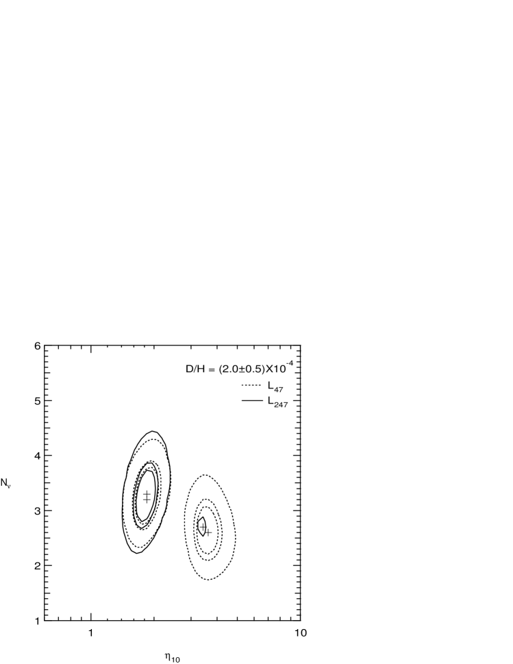
Figure 2: (a) 50%, 68% & 95% C.L. contours of $L_{47}$ and $L_{247}$ where observed abundances are given by eqs. (2, 3, and 4).

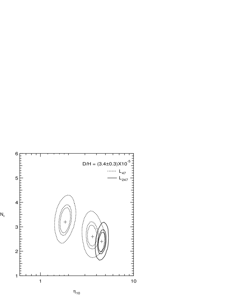
Figure 2: (b) 50%, 68% & 95% C.L. contours of $L_{47}$ and $L_{247}$ where observed abundances are given by eqs. (2, 3, and 5).

The peaks of the distribution as well as the allowed ranges of $\eta$ and $N_{\nu}$ are more easily discerned in the contour plots of Figure 2 which shows the 50%, 68% and 95% confidence level contours in $L_{47}$ and $L_{247}$. The crosses show the location of the peaks of the likelihood functions. Note that $L_{47}$ peaks at $N_{\nu}=3.2$, (up slightly from the case with $\hbox{$Y_{\rm p}$}=.234$) and $\eta_{10}=1.85$. The second peak of $L_{47}$ occurs at $N_{\nu}=2.6$, $\eta_{10}=3.6$. The 95% confidence level allows the following ranges in $\eta$ and $N_{\nu}$

$$1.7\leq N_{\nu}\leq 4.3$$

$$1.4\leq\eta_{10}\leq 4.9$$ (12)

These results differ only slight from those in [2].

Since $L_{2}$ picks out a small range of values of $\eta$, largely independent of $N_{\nu}$, its effect on $L_{247}$ is to eliminate one of the two peaks in $L_{47}$. With the high D/H value, $L_{247}$ peaks at the slightly higher value $N_{\nu}=3.3$, $\eta_{10}=1.85$. In this case the 95% contour gives the ranges

$$2.2\leq N_{\nu}\leq 4.4$$

$$1.4\leq\eta_{10}\leq 2.4$$ (13)

(Strictly speaking, $\eta_{10}$ can also be in the range 3.2—3.5, with $2.5\mathrel{\mathchoice{\lower 3.6pt\vbox{\halign{$\mathsurround=0pt\displaystyle\hfil#\hfil$\cr<\crcr\sim\crcr}}}{\lower 3.6pt\vbox{\halign{$\mathsurround=0pt\textstyle\hfil#\hfil$\cr<\crcr\sim\crcr}}}{\lower 3.6pt\vbox{\halign{$\mathsurround=0pt\scriptstyle\hfil#\hfil$\cr<\crcr\sim\crcr}}}{\lower 3.6pt\vbox{\halign{$\mathsurround=0pt\scriptscriptstyle\hfil#\hfil$\cr<\crcr\sim\crcr}}}}N_{\nu}\mathrel{\mathchoice{\lower 3.6pt\vbox{\halign{$\mathsurround=0pt\displaystyle\hfil#\hfil$\cr<\crcr\sim\crcr}}}{\lower 3.6pt\vbox{\halign{$\mathsurround=0pt\textstyle\hfil#\hfil$\cr<\crcr\sim\crcr}}}{\lower 3.6pt\vbox{\halign{$\mathsurround=0pt\scriptstyle\hfil#\hfil$\cr<\crcr\sim\crcr}}}{\lower 3.6pt\vbox{\halign{$\mathsurround=0pt\scriptscriptstyle\hfil#\hfil$\cr<\crcr\sim\crcr}}}}2.9$ as can be seen by the 95% contour in Figure 2a. However this “peak” is almost completely invisible in Figure 1b.) The 95% CL ranges in $N_{\nu}$ for both $L_{47}$ and $L_{247}$ include values below the canonical value $N_{\nu}=3$. Since one could argue that $N_{\nu}\geq 3$, we could use this condition as a Bayesian prior. This was done in [30] and in the present context in [2]. In the latter, the effect on the limit to $N_{\nu}$ was minor, and we do not repeat this analysis here.

In the case of low D/H, $L_{2}$ picks out a smaller value of $N_{\nu}=2.4$ and a larger value of $\eta=4.55$. The 95% CL upper limit is now $N_{\nu}<3.2$, and the range for $\eta$ is $3.9<\eta_{10}<5.4$. It is important to stress that with the increase in the determined value of D/H [17] in the low D/H systems, these abundances are now consistent with the standard model value of $N_{\nu}=3$ at the 2 $\sigma$ level.

Although we feel that the above set of values represents the current best choices for the observational parameters, our real goal in this paper is to generalize these results for a wide range of possible primordial abundances. To begin with, we will fix (Li/H)_p from Eq. (3), and allow $Y_{\rm p}$ to vary from 0.225 – 0.250. In Figure 3, the positions of the two peaks of the likelihood function, $L_{47}$, are shown as functions of $Y_{\rm p}$. The low-$\eta$ peak is shown by the dashed curve, while the high-$\eta$ peak is shown as dotted. The preferred value of $N_{\nu}=3$, corresponds to a peak of the likelihood function either at $\hbox{$Y_{\rm p}$}=0.234$ at low $\eta_{10}=1.8$ or at $\hbox{$Y_{\rm p}$}=0.243$ at $\eta_{10}=3.6$ (very close to the value of $Y_{\rm p}$ quoted in [19]). Since the peaks of the likelihood function are of comparable height, no useful statistical information can be extracted concerning the relative likelihood of the two peaks. The 95% CL upper limit to $N_{\nu}$ as a function of $Y_{\rm p}$ is shown by the solid curve, and over the range in $Y_{\rm p}$ considered varies from 3.3 – 5.3. The fact that the peak value of $N_{\nu}$ (and its upper limit) increases with $Y_{\rm p}$ is easy to understand. The BBN production of ⁴He increases with increasing $N_{\nu}$. Thus for fixed Li/H, or fixed $\eta$, raising $Y_{\rm p}$ must be compensated for by raising $N_{\nu}$ in order to avoid moving the peak likelihood to higher values of $\eta$ and therefore off of the ⁷Li peak.

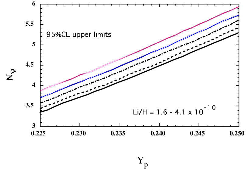
Figure 5: Summary of the upper limits to $N_{\nu}$ for (Li/H)${}_{p}=1.6,2.0,2.6,3.2,{\rm and}\ 4.1\times 10^{-10}$ as a function of $Y_{\rm p}$. The lowest curve corresponds to (Li/H)${}_{p}=1.6\times 10^{-10}$ and the limits on $N_{\nu}$ increase with (Li/H)_p.

In Figure 4, we show the corresponding results with (Li/H)${}_{p}=4.1\times 10^{-10}$. In this case, we must assume that lithium was depleted by a factor of $\sim 2.5$ or 0.4 dex, corresponding to the upper limit derived in [9]. The effect of assuming a higher value for the primordial abundance of Li/H is that the two peaks in the likelihood function are split apart. Now the value of $N_{\nu}=3$ occurs at $\hbox{$Y_{\rm p}$}=0.227$ at $\eta_{10}=1.1$ (a very low value) and at $\hbox{$Y_{\rm p}$}=0.248$ and $\eta_{10}=5.7$. The 95% CL upper limit on $N_{\nu}$ in this case can even extend up to 6 at $\hbox{$Y_{\rm p}$}=0.250$. In Figure 5, we show a compilation of the 95% CL upper limits to $N_{\nu}$ for different values of (Li/H)${}_{p}=1.6,2.0,2.6,3.2,{\rm and}~{}4.1\times 10^{-10}$. The upper limit to $N_{\nu}$ can be approximated by a fit to our results which can be expressed as

$$N_{\nu}\mathrel{\mathchoice{\lower 3.6pt\vbox{\halign{$\mathsurround=0pt\displaystyle\hfil#\hfil$\cr<\crcr\sim\crcr}}}{\lower 3.6pt\vbox{\halign{$\mathsurround=0pt\textstyle\hfil#\hfil$\cr<\crcr\sim\crcr}}}{\lower 3.6pt\vbox{\halign{$\mathsurround=0pt\scriptstyle\hfil#\hfil$\cr<\crcr\sim\crcr}}}{\lower 3.6pt\vbox{\halign{$\mathsurround=0pt\scriptscriptstyle\hfil#\hfil$\cr<\crcr\sim\crcr}}}}80\hbox{$Y_{\rm p}$}+2.5\times 10^{9}{\rm(Li/H)}_{p}-15.15$$ (14)

Finally we turn to the cases when D/H from quasar absorption systems are also considered in the analysis. For the high D/H given in Eq. (4), though there is formally still a high-$\eta$ peak, the value of the likelihood function $L_{247}$ there is so low that it barely falls within the 95% CL equal likelihood contour (see Figures 1b and 2a). Therefore we will ignore it here. In Figure 6, we show the peak value of $N_{\nu}$ and its upper limit for the two cases of (Li/H)${}_{p}=1.6$ and $4.1\times 10^{-10}$. These results differ only slightly from those shown in Figures 3 and 4. We note however, that overall the two values of Li/H do not give an equally good fit. For fixed D/H, the high value prefers a value of $\eta_{10}\simeq 1.8$ coinciding with the position of the low-$\eta$ peak for (Li/H)${}_{p}=1.6\times 10^{-10}$. At higher Li/H, the low-$\eta$ peak shifts to lower $\eta$ diminishing the overlap with D/H. In fact at (Li/H)${}_{p}\mathrel{\mathchoice{\lower 3.6pt\vbox{\halign{$\mathsurround=0pt\displaystyle\hfil#\hfil$\cr>\crcr\sim\crcr}}}{\lower 3.6pt\vbox{\halign{$\mathsurround=0pt\textstyle\hfil#\hfil$\cr>\crcr\sim\crcr}}}{\lower 3.6pt\vbox{\halign{$\mathsurround=0pt\scriptstyle\hfil#\hfil$\cr>\crcr\sim\crcr}}}{\lower 3.6pt\vbox{\halign{$\mathsurround=0pt\scriptscriptstyle\hfil#\hfil$\cr>\crcr\sim\crcr}}}}3.8\times 10^{-10}$, the likelihood function $L_{247}$ takes peak values which would lie outside the 95% CL contour of the case (Li/H)${}_{p}=1.6\times 10^{-10}$. The relative values of the likelihood function $L_{247}$, on the low-$\eta$ peak, for the five values of Li/H considered are shown in Figure 7. Contrary to our inability to statistically distinguish between the two peaks of $L_{47}$, the large variability in the values of $L_{247}$ shown in Figure 7 are statistically relevant. Thus, as claimed in [4], if the high D/H could be confirmed, one could set a strong limit on the amount of ⁷Li depletion in halo dwarf stars.

Since the low D/H value has come up somewhat, and since here we are considering the possibility for higher values of $Y_{\rm p}$ and (Li/H)_p, the statistical treatment of the low D/H case is warranted. In Figure 8, we show the peak value and 95% CL upper limit from $L_{247}$ when the low value of D/H is used from Eq. (5) with (Li/H)${}_{p}=1.6\times 10^{-10}$. The results are not significantly different in this case for the other choices of (Li/H)_p. In order to obtain $N_{\nu}=3$, one needs to go to ⁴He abundances as high as $\hbox{$Y_{\rm p}$}=0.247$ with respect to the peak of the likelihood function. However, for $Y_{p}>0.234$, the revised low value of D/H is compatible with ⁴He and ⁷Li at the 95% CL. The likelihood functions $L_{247}$ are shown in Figure 9 for completeness.

5 Conclusions

We have generalized the full two-dimensional (in $\eta$ and $N_{\nu}$) likelihood analysis based on big bang nucleosynthesis for a wide range of possible primordial abundances of ⁴He and ⁷Li. Allowing for full freedom in both the baryon-to-photon ratio, $\eta$, and the number of light particle degrees of freedom as characterized by the number of light, stable neutrinos, $N_{\nu}$, we have updated the allowed range in $\eta$ and $N_{\nu}$ based the higher value of $Y_{p}=0.238\pm 0.002\pm 0.005$ from [20] which includes the recent data in [19]. The likelihood analysis based on ⁴He and ⁷Li yields the 95% CL upper limits: $N_{\nu}\leq 4.3$ and $\eta_{10}\leq 4.9$. The result for $N_{\nu}$ is only slightly altered, $N_{\nu}\leq 4.4$, when the high values of D/H observed in certain quasar absorption systems [14, 16] are included in the analysis. In this case, the upper limit to $\eta_{10}$ is lowered to 2.4. Since the low values of D/H have been revised upward somewhat [15], they are now consistent with ⁴He and ⁷Li and $N_{\nu}=3$ at the 95% CL. We have also shown how our results for the upper limit to $N_{\nu}$ depend on the specific choice for the primordial abundance of ⁴He and ⁷Li. If we assume that the observational determination of ⁷Li in halo stars is a true indicator the primordial abundance of ⁷Li, then the upper limit to $N_{\nu}$ varies from 3.3 – 5.3 for $Y_{\rm p}$ in the range 0.225 – 0.250. If on the other hand, ⁷Li is depleted in halo stars by as much as a factor of 2.5, then the upper limit to $N_{\nu}$ could extend up to 6 at $\hbox{$Y_{\rm p}$}=0.250$.

Acknowledgments We note that this work was begun in collaboration with David Schramm. This work was supported in part by DOE grant DE-FG02-94ER40823 at Minnesota.

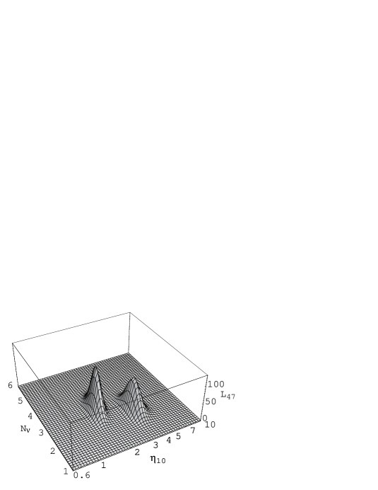
Figure 1: (a) $L_{47}(N_{\nu},\eta)$ for observed abundances given by eqs. (2 and 3).

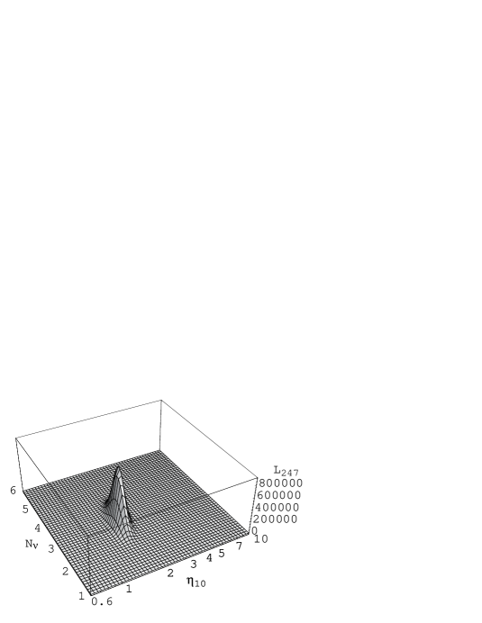
Figure 1: (b) $L_{247}(N_{\nu},\eta)$ for observed abundances given by eqs. (2, 3, and 4).

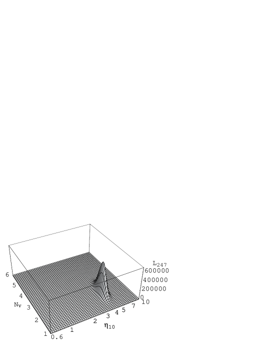
Figure 1: (c) $L_{247}(N_{\nu},\eta)$ for observed abundances given by eqs. (2, 3, and 5).

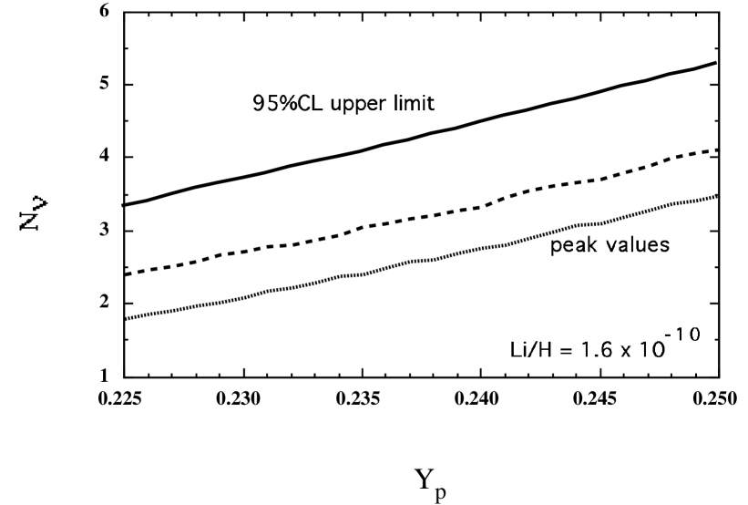
Figure 3: The position of the value of $N_{\nu}$ along the low-$\eta$ peak (dashed) and high-$\eta$ peak (dotted) of the likelihood function $L_{47}$ as function of $Y_{\rm p}$. The solid curve shows the 95% CL upper limit to $N_{\nu}$ as a function of $Y_{\rm p}$. The value of (Li/H)${}_{p}=1.6\times 10^{-10}$ has been fixed.

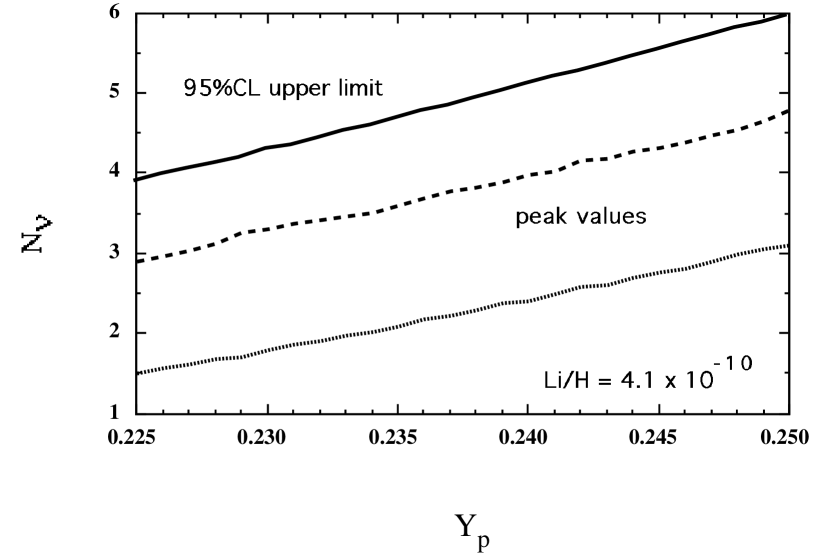
Figure 4: As in Figure 3 with (Li/H)${}_{p}=4.1\times 10^{-10}$.

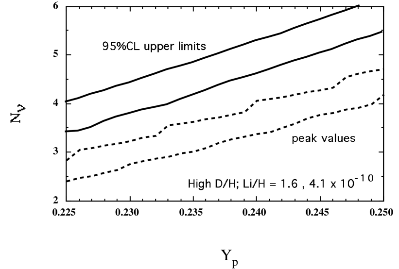
Figure 6: As in Figures 3 and 4 based on the likelihood function $L_{247}$ which includes high D/H from quasar absorption systems.

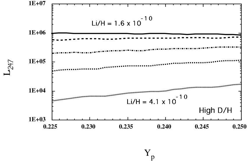
Figure 7: Relative values of the likelihood function $L_{247}$, on the low-$\eta$ peak, for the five choices of (Li/H)_p in Figure 5.

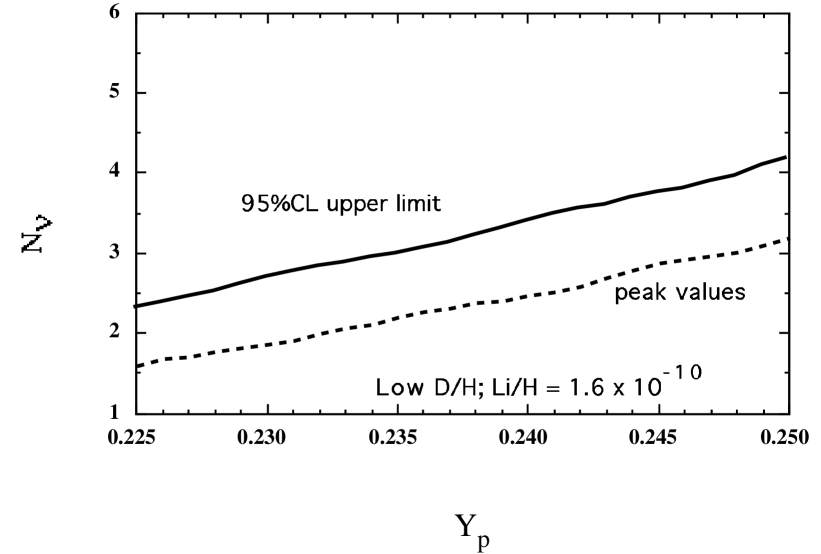
Figure 8: As in Figure 6 for low D/H from quasar absorption systems.

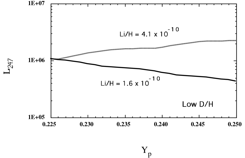
Figure 9: As in Figure 7 for low D/H from quasar absorption systems.

References

- [1] G. Steigman, D.N. Schramm, and J. Gunn, Phys. Lett. B66 (1977) 202.
- [2] K.A. Olive and D. Thomas, AstroPart. Phys. 7 (1997) 27.
- [3] B.D. Fields, and K.A. Olive, Phys. Lett. B368 (1996) 103.
- [4] B.D. Fields, K. Kainulainen, K.A. Olive, and D. Thomas, New Astr. 1 (1996) 77.
- [5] C.J. Copi, D.N. Schramm, and M.S. Turner, Phys. Rev. D55 (1997) 3389; N. Hata, G. Steigman, S. Bludman and P. Langacker, Phys. Rev. D55 (1997) 540.
- [6] K.A. Olive, E. Skillman, and G. Steigman, Ap.J. 483 (1997) 788.
- [7] P. Molaro, F. Primas, and P. Bonifacio, A.A. 295 (1995) L47; P. Bonifacio and P. Molaro, MNRAS, 285 (1997) 847.
- [8] Y.I. Izotov, T.X. Thuan, and V.A. Lipovetsky, Ap.J. 435 (1994) 647; Ap.J.S. 108 (1997) 1.
- [9] M.H. Pinsonneault, T.P. Walker, G. Steigman, and V.K. Naranyanan, Ap.J. (1998) submitted, astro-ph/9803073.
- [10] K.A. Olive, R.T. Rood, D.N. Schramm, J.W. Truran, and E. Vangioni-Flam, Ap.J. 444 (1995) 680; D. Galli, F. Palla, F. Ferrini, and U. Penco, Ap.J. 443 (1995) 536; D. Dearborn, G. Steigman, and M. Tosi, Ap.J. 465 (1996) 887; S.T. Scully, M. Cassé, K.A. Olive, D.N. Schramm, J. Truran, and E. Vangioni-Flam, Ap.J. 462 (1996) 960; K.A. Olive, S.T. Scully, D.N. Schramm, and J. Truran, Ap.J. 479 (1996) 752.
- [11] S. Scully, M. Cassé, K.A. Olive, E. Vangioni-Flam, Ap. J. 476 (1997) 521.
- [12] S.J. Lilly, O. Le Fevre, F. Hammer, and D. Crampton, Ap.J. 460 (1996) L1; P. Madau, H.C. Ferguson, M.E. Dickenson, M. Giavalisco, C.C. Steidel, and A. Fruchter, MNRAS 283 (1996) 1388; A.J. Connolly, A.S. Szalay, M. Dickenson, M.U. SubbaRao, and R.J. Brunner, Ap.J. 486 (1997) L11; M.J. Sawicki, H. Lin, and H.K.C. Yee, A.J. 113 (1997) 1.
- [13] M. Cassé, K.A. Olive, E. Vangioni-Flam, and J. Audouze, New Astronomy 3 (1998) 259.
- [14] R.F. Carswell, M. Rauch, R.J. Weymann, A.J. Cooke, and J.K. Webb, MNRAS 268 (1994) L1; A. Songaila, L.L. Cowie, C. Hogan, and M. Rugers, Nature 368 (1994) 599.
- [15] D. Tytler, X.-M. Fan, and S. Burles, Nature 381 (1996) 207; S. Burles and D. Tytler, Ap.J. 460 (1996) 584.
- [16] J.K. Webb, R.F. Carswell, K.M. Lanzetta, R. Ferlet, M. Lemoine, A. Vidal-Madjar, and D.V. Bowen, Nature 388 (1997) 250; D. Tytler et al., astro-ph/9810217 (1998).
- [17] S. Burles and D. Tytler, Ap.J. 499 (1998) 699; Ap.J. 507 (1998) 732.
- [18] C. Copi, K.A. Olive, and D.N. Schramm, Proc. Nat. Ac. Sci. 95 (1998) 2758, astro-ph/9606156.
- [19] Y.I. Izotov, and T.X. Thuan, ApJ, 500 (1998) 188.
- [20] B.D. Fields and K.A. Olive, Ap.J. 506 (1998) 177.
- [21] B.E.J. Pagel, E.A. Simonson, R.J. Terlevich and M. Edmunds, MNRAS 255 (1992) 325; E. Skillman, and R.C. Kennicut, ApJ, 411 (1993) 655; E. Skillman, R.J. Terlevich, R.C. Kennicutt, D.R. Garnett, and E. Terlevich, ApJ, 431(1994) 172.
- [22] G. Steigman, B. Fields, K.A. Olive, D.N. Schramm, and T.P. Walker, Ap.J. 415 (1993) L35; M. Lemoine, D.N. Schramm, J.W. Truran, and C.J. Copi, Ap.J. 478 (1997) 554; B.D. Fields and K.A. Olive, astro-ph/9811183, New Astronomy, in press (1998).
- [23] M. Rugers and C.J. Hogan, Ap.J. 459 (1996) L1.
- [24] L.M. Krauss and P. Romanelli, ApJ, 358 (1990) 47.
- [25] M. Smith, L. Kawano, and R.A. Malaney, Ap.J. Supp., 85 (1993) 219.
- [26] P.J. Kernan and L.M. Krauss, Phys. Rev. Lett. 72 (1994) 3309.
- [27] L.M. Krauss and P.J. Kernan, Phys. Lett. B347 (1995) 347.
- [28] N. Hata, R.J. Scherrer, G. Steigman, D. Thomas, and T.P. Walker, Ap.J., 458 (1996) 637.
- [29] N. Hata, R. J. Scherrer, G. Steigman, D. Thomas, T. P. Walker, S. Bludman and P. Langacker, Phys. Rev. Lett. 75 (1995) 3977.
- [30] K.A. Olive and G. Steigman, Phys. Lett. B354 (1995) 357.