DESY 98-136

Doubly Charged Higgsino Pair Production and Decays
in ${\bf e^{+}e^{-}}$ Collisions

M. Raidal and P.M. Zerwas

DESY, Deutsches Elektronen-Synchrotron, D–22603 Hamburg, Germany

In supersymmetric grand unified theories, light higgsino multiplets generally exist in addition to the familiar chargino/neutralino multiplets of the minimal supersymmetric extension of the Standard Model. The new multiplets may include doubly charged states $\tilde{\Delta}^{\pm\pm}$ and $\tilde{\delta}^{\pm\pm}$. We study the properties and the production channels of these novel higgsinos in $e^{+}e^{-}$ and $\gamma\gamma$ collisions, and investigate how their properties can be analyzed experimentally.

1. Synopsis

While the Standard Model (SM) has been extremely successful in interpreting nearly all experimental observations in the past three decades, there is increasing experimental evidence that the model should be embedded in a more comprehensive theory. The deficit of solar and atmospheric neutrino fluxes and indications for the existence of hot and cold components of dark matter point clearly to directions of physics beyond the Standard Model [1].

Strongly motivated by the observations of non–zero neutrino masses, the embedding of the SM in a left–right (LR) symmetric grand unified theory (GUT) like $SO(10)$ [2, 3] or $E_{6}$ [4] is a most attractive direction. In this approach, the chiral fermion fields of one generation are grouped together in a single multiplet of the fundamental representation, including the right–handed neutrino component.

The hierarchy problem, related to light fundamental scalars in the context of very high GUT scales, is partly solved, in a natural way, by extending the model to a supersymmetric (SUSY) theory. The non–trivial vacuum structure and the breaking of supersymmetry leads to interesting new phenomena. In SUSY GUT-s with intermediate left–right symmetry, novel light superfields can be present despite the very high scale of the left–right symmetry breaking [5, 6, 7]. The resulting low–energy theory is the $R$–parity conserving minimal supersymmetric standard model (MSSM), supplemented by light massive neutrinos which can be generated by the see–saw mechanism [8], and light remnants of the Higgs supermultiplets. If the scale for left–right symmetry breaking is chosen such as to generate the right order of neutrino masses, the new light states should have masses in the range of $\sim$ 100 GeV.

In this study we focus on one of the central predictions of this type of SUSY models in the light fermionic higgsino sector: light doubly charged $SU(2)_{L}\times U(1)_{Y}$ triplet components $\tilde{\Delta}^{++}$ and singlets $\tilde{\delta}^{++}$. We construct the effective low–energy model incorporating these new fields and define their interactions. The influence of the new particles on the unification of couplings is studied in the context of SUSY SO(10). Subsequently we work out the phenomenology of these particles at future $e^{+}e^{-}$ linear colliders, extending earlier work in Refs.[9, 10]:

$$e^{+}e^{-} \rightarrow \tilde{\Delta}^{++}\tilde{\Delta}^{--}$$ (1)

$$e^{+}e^{-} \rightarrow \tilde{\delta}^{++}\tilde{\delta}^{--}$$ (2)

We will discuss the production of the doubly charged higgsinos and their decay modes. Final–state correlations among the decay products, rooted in spin–spin correlations, can be exploited to measure the fundamental couplings of these particles [12]. $\gamma\gamma$ collisions which are particularly suited for the production of doubly charged particles will also be briefly commented.

The outline of the paper is as follows. After describing the general physics base in Section 2, the production of higgsinos will be presented in Section 3, followed by a discussion of the decay modes in the subsequent section. In Section 5, angular correlations will be exploited to determine the higgsino couplings.

2. Effective Low–Energy Theory

Grand unified theories which incorporate left–right symmetries, include the groups $SO(10)$ and $E_{6}$. If broken down to the Standard Model gauge group $SU(2)_{L}\times U(1)_{Y}$, effective theories based on intermediate $SU(2)_{L}\times SU(2)_{R}\times U(1)_{B-L}$ or other symmetries may be realized at a scale $M_{R}$. Embedding such models in supersymmetric theories can solve many of the problems of the MSSM: strong and weak CP problems; the conservation of $R$ parity [13]. These theories can also accommodate small neutrino masses through the see–saw mechanism in a natural way.

Several theoretical possibilities exist in SUSY LR models [14] which lead, after symmetry breaking, to vacua conserving the electric charge. (i) Either the LR breaking scale must be low, $M_{R}\mathrel{\vbox{\hbox{$<$}\nointerlineskip\hbox{$\sim$}}}M_{SUSY}$, and $R$–parity must be spontaneously broken at the same time [15]; or (ii) $B-L$ neutral triplets must be added; or (iii) non–renormalizable interactions must be introduced [5, 6]. The phenomenomena emerging from (i) have been studied in Ref.[16]. The scenario (ii) may lead to new light singly charged higgsinos. In this paper, we concentrate specifically on phenomena following from the third solution which involves doubly charged spin–1/2 particles.

This solution implies that the right–handed symmetry breaking scale is very high, $M_{R}\mathrel{\vbox{\hbox{$>$}\nointerlineskip\hbox{$\sim$}}}{\cal O}(10^{10}-10^{11}$ GeV). At such a scale effective higher-order operators originating from Planck scale physics may start playing a role. Since the scale $M_{R}$ sets the natural mass scale of the new particles, one may naïvely guess that all the new particles decouple from the low–mass spectrum. However, as a result of the vacuum structure, the decoupling is not complete in supersymmetric theories. (This was already noticed quite early in Ref.[17]). If the supersymmetry is unbroken, the symmetry leads to an ensemble of degenerate vacua corresponding to flat directions. The excitations associated with these flat directions are massless particles. If SUSY is broken, the $D$–flat directions are lifted and the theory picks one of the vacua; if $R$–parity is conserved and $M_{R}$ is sufficiently high [18], the vacuum conserves the electric charge [5, 6]. The previously massless excitations are transformed to states with masses of order $m\sim M^{2}_{R}/M_{PL}$, with $M_{PL}$ being the Planck scale. Besides the light neutrinos, the effective low–energy theory will include these light remnants in addition to the MSSM particle spectrum.

In this scenario the effective low–energy theory is defined by the MSSM with exact $R$–parity, supplemented by two left–handed triplet superfields $\Delta$ and $\bar{\Delta}$, and two right-handed singlet superfields $\delta$ and $\bar{\delta}$ with opposite $U(1)$ quantum numbers such as to cancel chiral anomalies. They are assigned the $SU(2)_{L}\times U(1)_{Y}$ quantum numbers

$$\Delta=\left(\begin{array}[]{cc}\Delta^{+}/\sqrt{2}&\Delta^{++}\\ \Delta^{0}&-\Delta^{+}/\sqrt{2}\end{array}\right)=(3,2) \bar{\Delta}=\left(\begin{array}[]{cc}\bar{\Delta}^{-}/\sqrt{2}&\bar{\Delta}^{0}\\ \bar{\Delta}^{--}&-\bar{\Delta}^{-}/\sqrt{2}\end{array}\right)=(3,-2)$$ (7)

and

$$\delta=\delta^{--}=(1,-4)\;\;\;\;\;\;\;\;\;\;\;\;\; \bar{\delta}=\bar{\delta}^{++}=(1,4)$$ (8)

These fields are the light remnants of the Higgs supermultiplets in the underlying GUT theory belonging to (3,1) and (1,3) representation of the intermediate $SU(2)_{L}\times SU(2)_{R}$ subgroup, respectively. The superpotential, apart from the non-renormalizable terms, may be written as

$$W=W_{MSSM}+W_{T}+W_{S}$$ (9)

where $W_{MSSM}$ is the superpotential of the MSSM [19] and the new terms $W_{T}$ and $W_{S}$ describing the triplet and singlet superfield interactions, respectively, are given by

$$W_{T} = M_{\Delta}\mbox{\rm Tr}\Delta\bar{\Delta}+if_{\Delta}L^{T}\tau_{2}\Delta L\,,$$

$$W_{S} = M_{\delta}\delta^{--}\bar{\delta}^{++}+f_{\delta}l^{c}l^{c}\delta^{--}$$ (10)

The doublet of left-handed leptons is denoted by $L$ and the singlet of the right-handed lepton by $l^{c}$ ($f_{\delta}=f_{\Delta}$ for strict LR symmetry at the relevant scale). Because of stringent constraints on lepton–flavor violation from the processes $l_{1}\to l_{2}\gamma,$ $l_{1}\to 3l_{2}$ and $\mu-e$ conversion in nuclei, the couplings $f$ are diagonal to a high degree of accuracy in family space [20]. The experimental bound from muonium-antimuonium conversion implies the constraint $f_{ee}f_{\mu\mu}\mathrel{\vbox{\hbox{$<$}\nointerlineskip\hbox{$\sim$}}}1.2\cdot 10^{-3}$ for the mass $M_{\Delta}=100$ GeV while no constraints can be set on the coupling $f_{\tau\tau}.$ This implies that light doubly charged particles with masses around 100 GeV cannot decay to electrons and muons at the same time.

Including new light supermultiplets (7,8) in the low–energy particle spectrum will influence the running of couplings and may dangerously spoil the unification of $\alpha_{1}=3/5\alpha_{Y},$ $\alpha_{2}$ and $\alpha_{3}=\alpha_{s}$ at the GUT scale [21], eventually jeopardizing the unification of the couplings, or worse, driving the unification point to a dangerously low scale for proton decay. The evolution of couplings to one–loop order is described by the solutions of the renormalization group equations,

$$\frac{1}{\alpha_{i}(M_{X})}=\frac{1}{\alpha_{i}(\mu)}+\frac{b_{i}}{2\pi}\ln\left(\frac{\mu}{M_{X}}\right)$$ (11)

where the beta functions $b_{i}$ depend on the particle content of the theory.

Figure 1: Running of the coupling constants assuming the intermediate Pati-Salam partial unification.

We shall exemplify a possible symmetry breaking path by assuming $SO(10)$ as grand unification group broken down to the SM symmetry in the Pati–Salam chain:

$$SO(10) \longrightarrow\!\!\!\!\!\!\!\!\!\!\!^{M_{U}} SU(4)\times SU(2)_{R}\times SU(2)_{L}$$ (12)

$$\longrightarrow\!\!\!\!\!\!\!\!\!\!^{M_{R}} SU(3)_{c}\times SU(2)_{L}\times U(1)_{Y}$$

$$\longrightarrow\!\!\!\!\!\!\!\!\!\!\!^{M_{W}} SU(3)_{c}\times U(1)_{em}$$

At the scale $M_{R}$ the couplings must satisfy the boundary conditions for Pati-Salam partial unification:

$$\alpha^{-1}_{3}(M_{R}) = \alpha^{-1}_{4}(M_{R})$$

$$\alpha^{-1}_{2}(M_{R}) \equiv \alpha^{-1}_{2L}(M_{R})=\alpha^{-1}_{2R}(M_{R})$$

$$\alpha^{-1}_{1}(M_{R}) = \frac{3}{5}\alpha^{-1}_{2}(M_{R})+\frac{2}{5}\alpha^{-1}_{3}(M_{R})$$ (13)

While the first two conditions are self–evident, the third condition follows from the breaking mechanism $R\times(B-L)\to Y.$ The partial unification scale is fixed by the third condition. The low energy particle spectrum at scales $M_{X}$ below $M_{R}$ is already specified in eq.(9). The corresponding SUSY beta functions $b_{i}$ are given by

$$b_{1} = 2N_{F}+\frac{3}{10}N_{D}+\frac{9}{5}N_{\Delta}+\frac{12}{5}N_{\delta}$$

$$b_{2L} = -6+2N_{F}+\frac{1}{2}N_{D}+2N_{\Delta}$$

$$b_{3} = -6+2N_{F}$$ (14)

where $N_{F}=3$ is the number of families, and $N_{D},$ $N_{\Delta}$ and $N_{\delta}$ are the numbers of doublet, triplet and singlet Higgs superfields, respectively; in the present example, $N_{D}=N_{\Delta}=N_{\delta}=2.$ The additional light Higgs superfields increase the slopes of $\alpha_{1}^{-1}$ and $\alpha_{2}^{-1},$ and they accelerate the running of the two couplings. Above $M_{R},$ the minimal $SU(2)_{L,R}$ superfield content is naturally assumed to consist of two doublets, and of two left–handed and two right–handed triplets [$\Delta/\bar{\Delta}$ and $\delta/\bar{\delta},$ respectively]. This spectrum implies for the beta functions $b_{2L,R}$

$$b_{2L}=b_{2R}=-6+2N_{F}+\frac{1}{2}N_{D}+2N_{\Delta,\delta}$$ (15)

$\alpha_{2L}^{-1}=\alpha_{2}^{-1}$ therefore evolves with $M_{X}$ without any break across the scale $M_{R}$, cf. Fig.1. Since the coupling $\alpha_{3}^{-1}$ becomes larger than $\alpha_{2}^{-1}$ near $M_{R}$, the asymptotically free color $SU(3)_{c}$ sector must transmute into an asymptotically non–free Pati–Salam $SU(4)$ sector at $M_{R}$ in order to evolve into a grand unification crossing point with $SU(2)_{L}\times SU(2)_{R}$ at a large scale $M_{U}\mathrel{\vbox{\hbox{$>$}\nointerlineskip\hbox{$\sim$}}}10^{16}$ GeV. This can be achieved by introducing $N_{10}$ ten-plet superfields, giving rise to the beta function

$$b_{4}=-12+2N_{g}+3N_{10}$$ (16)

Four such ten–plets are needed at least, in the present example, to reach a unification point below the Planck scale; with $N_{10}=4$ the $SO(10)$ unification point $M_{U}$ is located at a scale $M_{U}\sim 10^{16}$ GeV while the LR symmetry breaking scale is $M_{R}\sim 10^{10}$ GeV, given the standard low energy couplings at $M_{Z}.$

Even though this specific example may look somewhat baroque, as a result of the little motivated ten–plet spectrum, it demonstrates nevertheless that light Higgs superfields can be accommodated in grand–unification $SO(10)$ scenarios indeed.

The two–component mass terms for the doubly charged higgsinos are derived from the superpotential (10),

$${\cal L}_{mass}=-M_{\tilde{\Delta}}\tilde{\Delta}^{++}_{L}\tilde{\bar{\Delta}}^{--}_{L}-M_{\tilde{\delta}}\tilde{\delta}^{--}_{R}\tilde{\bar{\delta}}^{++}_{R}+h.c.$$ (17)

where the tilde denotes the fermionic component of the corresponding superfield in eq.(7). It follows from the above Lagrangean that the fermionic components of the two triplet (and singlet) superfields combine to form one four–component fermion Dirac field; $\tilde{\Delta}^{++}_{L}$ and $(\tilde{\bar{\Delta}}^{--}_{L})^{c}=\tilde{\bar{\Delta}}^{++}_{R}$ can be identified as left– and right–chiral components of one Dirac field $\tilde{\Delta}^{++}$ [$\tilde{\delta}$ correspondingly]. Therefore the left- and right-chirality components of the four–component fermions, $\tilde{\Delta}^{++}_{L,R}$ and $\tilde{\delta}^{++}_{L,R},$ carry the same $SU(2)_{L}$ iso–quantum numbers and they couple not only to the photon but also to the $Z$-boson in exactly the same way.

The gauge interactions of the new higgsinos are described by the usual Lagrangean

$${\cal L}=\overline{\tilde{\Delta}^{++}_{L}}i\!\!\not\!\!D\tilde{\Delta}^{++}_{L}+\overline{\tilde{\Delta}^{++}_{R}}i\!\!\not\!\!D\tilde{\Delta}^{++}_{R}+\overline{\tilde{\delta}^{++}_{L}}i\!\!\not\!\!D\tilde{\delta}^{++}_{L}+\overline{\tilde{\delta}^{++}_{R}}i\!\!\not\!\!D\tilde{\delta}^{++}_{R}$$ (18)

where the covariant derivative is given by $iD_{\mu}=i\partial_{\mu}+eQ_{\gamma}A_{\mu}+g_{Z}Q_{Z}Z_{\mu}$ with $g_{Z}=e/(s_{W}c_{W}).$ $Q_{\gamma}$ is the electric charge related to isospin $I_{3}$ and hypercharge $Y$ by the Gell–Mann–Nishijama relation $Q_{\gamma}=I_{3}+Y/2$ while the $Z$–charge follows from $Q_{Z}=I_{3}-s^{2}_{W}Q_{\gamma}$ with $s^{2}_{W}=1-c^{2}_{W}=\sin^{2}\theta_{W}$ being the weak mixing angle. Both left– and right–chiral components of $\tilde{\Delta}^{++}$ and $\tilde{\delta}^{++}$ carry the same isospin $I_{3}=+1$ and $I_{3}=0$, respectively. The electroweak gauge theory of these fields is of vector–like character.

The relevant Yukawa interactions for the doubly charged higgsinos are given by the four–component Lagrangean

$${\cal L}_{Y}=-2f_{\Delta}\bar{l}^{c}_{L}\tilde{\Delta}^{++}_{L}\tilde{\l}_{L}-2f_{\delta}\bar{l}^{c}_{R}\tilde{\delta}^{++}_{R}\tilde{\l}_{R}+h.c.$$ (19)

where the subscripts $L,R$ denote the chirality of the fermions and the type of the sleptons at the same time.

It is instructive to analyze also the chargino and neutralino sectors of the model in toto. Due to the two new triplets, three charginos are generated,

$$\psi^{+} = \left(-i\tilde{\omega}^{+},\tilde{h}_{2}^{+},\tilde{\Delta}^{+}\right)$$ (20)

$$\psi^{-} = \left(-i\tilde{\omega}^{-},\tilde{h}_{1}^{-},\tilde{\bar{\Delta}}^{-}\right)$$ (21)

and six two component neutralinos,

$$\psi^{0}=\left(-i\tilde{b}^{0},-i\tilde{\omega}_{3}^{0},\tilde{h}_{1}^{0},\tilde{h}_{2}^{0},\tilde{\Delta}^{0},\tilde{\bar{\Delta}}^{0}\right)$$ (22)

However, the new states do not mix with the MSSM states. Because there is no doublet-triplet mixing in the superpotential, the doublet higgsinos do not mix with the triplet higgsinos. Triplets can, in principle, mix with gauginos due to the gauge-matter interactions

$${\cal L}_{int}=ig_{a}\sqrt{2}T^{a}_{ij}\phi_{i}^{*}\tilde{\omega}^{a}\psi_{j}+h.c.$$ (23)

where $T^{a}$ are the gauge group generators. However, the gaugino-triplet higgsino mixing terms are proportional to the vacuum expectation value $v_{L}$ of the neutral left-handed triplet Higgs field $\Delta^{0}$ which is strongly constrained from the measurement of the $\rho$ parameter to be below 1 GeV. Therefore these mixing terms are negligible and the triplet higgsino decouples from the MSSM states. The only mass term for the triplet neutralino generated by the superpotential (10) is of the type $\Delta^{0}\bar{\Delta}^{0}$ which implies that the components form one neutral Dirac fermion while the MSSM neutralinos are in general Majorana states. As a result, the interactions of the triplet higgsinos are limited to the Yukawa interactions of the type eq.(19) and to the gauge interactions. They do not mix with the MSSM states and the properties of the genuine charginos and neutralinos in the MSSM are not modified.

3. Production of Doubly Charged Higgsinos

The matrix elements of the processes (1) and (2) can, quite generally, be expressed in terms of four bilinear charges [23, 12], classified according to the chiralities $\alpha,\beta=L,R$ of the associated lepton and higgsino currents,

$$T\left(e^{+}e^{-}\rightarrow\tilde{\Delta}^{++}\tilde{\Delta}^{--}\right)=\frac{e^{2}}{s}Q_{\alpha\beta}\left[\bar{v}(e^{+})\gamma_{\mu}P_{\alpha}u(e^{-})\right]\left[\bar{u}(\tilde{\Delta}^{++})\gamma^{\mu}P_{\beta}v(\tilde{\Delta}^{--})\right]$$ (24)

and analogously for the process $e^{+}e^{-}\rightarrow\tilde{\delta}^{++}\tilde{\delta}^{--}.$ In this notation $\tilde{\Delta}^{++},$ $\tilde{\delta}^{++}$ are defined as particles and $\tilde{\Delta}^{--},$ $\tilde{\delta}^{--}$ as antiparticles.

Figure 2: Feynmam graphs for the production of $\tilde{\Delta}^{++}\tilde{\Delta}^{--}$ pair. The same set of diagrams describes $\tilde{\delta}^{++}\tilde{\delta}^{--}$ pair production with $\tilde{e}_{L}\to\tilde{e}_{R}$.

The process $e^{+}e^{-}\rightarrow\tilde{\Delta}^{++}\tilde{\Delta}^{--}$ is built up by $s$–channel $\gamma$ and $Z$ exchanges, and $t$–channel $\tilde{e}_{L}$ exchange. The corresponding Feynman diagrams are depicted in Fig.2. After the appropriate Fierz transformation, also the $t$–channel amplitude can be cast in the form of eq.(24). The charges for the process (1) are given by

$$e^{+}e^{-}\rightarrow\tilde{\Delta}^{++}\tilde{\Delta}^{--}:\,\,\;\;\;\;Q_{LL} = 1+2\cot^{2}2\theta_{W}D_{Z}+2(f_{\Delta}^{2}/e^{2})D_{\tilde{e}_{L}}$$

$$Q_{LR} = 1+2\cot^{2}2\theta_{W}D_{Z}$$

$$Q_{RR} = Q_{RL}\;=\;1-(\cos 2\theta_{W}/\cos^{2}\theta_{W})D_{Z}$$ (25)

The first index in $Q_{\alpha\beta}$ refers to the chirality of the $e^{\pm}$ current, the second index to the chirality of the $\tilde{\Delta}^{\pm\pm}$ current. In the process (1) the $\tilde{e}_{L}$ exchange affects only the $LL$ chirality charge while all other amplitudes are built up by $\gamma$ and $Z$ exchanges. $D_{\tilde{e}}$ denotes the slepton propagator $D_{\tilde{e}}=s/(t-m_{\tilde{e}}^{2})$, and $D_{Z}$ the $Z$ propagator $D_{Z}=s/(s-m^{2}_{Z}+im_{Z}\Gamma_{Z})$; the non–zero $Z$ width can in general be neglected for the energies considered in the present analysis so that the charges are real.

Figure 3: The polarized cross sections for the pair production of doubly charged higgsinos $\tilde{\Delta}^{\pm\pm}$ and $\tilde{\delta}^{\pm\pm}$ as functions of the collision energy. The choice of the masses, the Yukawa couplings and the electron beam polarizations (L/R=-/+) are indicated in the figures.

In contrast to (1), the process (2) describes the production of a right-handed singlet. The $\tilde{\delta}^{++}$ coupling to the $Z$ boson is modified according to eq.(18) and the $t$–channel exchange graph in Fig.2 involves the right–chiral selectron $\tilde{e}_{R}.$ The corresponding charges for the process $e^{+}e^{-}\rightarrow\tilde{\delta}^{++}\tilde{\delta}^{--}$ are given by

$$e^{+}e^{-}\rightarrow\tilde{\delta}^{++}\tilde{\delta}^{--}:\;\;\;\;\;Q_{LL} = Q_{LR}\;=\;1-(\cos 2\theta_{W}/\cos^{2}\theta_{W})D_{Z}$$

$$Q_{RL} = 1+2\tan^{2}\theta_{W}D_{Z}$$

$$Q_{RR} = 1+2\tan^{2}\theta_{W}D_{Z}+2(f_{\delta}^{2}/e^{2})D_{\tilde{e}_{R}}$$ (26)

As predicted by the chirality of $\tilde{\delta}^{++}$, the non-photonic contribution from the $t$–channel $\tilde{e}_{R}$ exchange affects only the $RR$ chirality charge.

To derive a transparent form for cross sections and polarization vectors, the following quartic charges are generally introduced,

$$Q_{1}=\frac{1}{4}\left[|Q_{RR}|^{2}+|Q_{LL}|^{2}+|Q_{RL}|^{2}+|Q_{LR}|^{2}\right]$$

$$Q_{2}=\frac{1}{2}{\rm Re}\left[Q_{RR}Q^{*}_{RL}+Q_{LL}Q^{*}_{LR}\right]$$

$$Q_{3}=\frac{1}{4}\left[|Q_{RR}|^{2}+|Q_{LL}|^{2}-|Q_{RL}|^{2}-|Q_{LR}|^{2}\right]$$ (27)

and

$$Q^{\prime}_{1}=\frac{1}{4}\left[|Q_{RR}|^{2}+|Q_{RL}|^{2}-|Q_{LR}|^{2}-|Q_{LL}|^{2}\right]$$

$$Q^{\prime}_{2}=\frac{1}{2}{\rm Re}\left[Q_{RR}Q^{*}_{RL}-Q_{LL}Q^{*}_{LR}\right]$$

$$Q^{\prime}_{3}=\frac{1}{4}\left[|Q_{RR}|^{2}+|Q_{LR}|^{2}-|Q_{RL}|^{2}-|Q_{LL}|^{2}\right]$$ (28)

which describe the independent experimental observables.

The final state probability may be expanded in terms of the unpolarized cross section, the polarization vectors of $\tilde{\Delta}^{++}$ and $\tilde{\Delta}^{--}$, and the spin–spin correlation tensor. The $\tilde{\Delta}^{++}$ production angle, with respect to the electron flight–direction, will be denoted by $\Theta$. Defining the $\hat{z}$ axis by the $e^{-}$ momentum, the $\hat{x}$ axis in the production plane with $\hat{x}\cdot\vec{p}_{\tilde{\Delta}^{++}}>0,$ and $\hat{y}=\hat{z}\times\hat{x}$ in the rest frame of the charginos, cross section and spin–density matrices are defined as [24]:

$$\frac{{\rm d}\sigma}{{\rm d}\cos\Theta}(\lambda\lambda^{\prime};\bar{\lambda}\bar{\lambda}^{\prime})=$$ (29)

$${}\hskip 5.69046pt=\frac{{\rm d}\sigma}{{\rm d}\cos\Theta}\frac{1}{4}\bigg{[}(I)_{\lambda^{\prime}\lambda}(I)_{\bar{\lambda}\bar{\lambda}^{\prime}}+{\cal P}_{i}(\tau^{i})_{\lambda^{\prime}\lambda}(I)_{\bar{\lambda}\bar{\lambda}^{\prime}}+\bar{\cal P}_{i}(I)_{\lambda^{\prime}\lambda}(\tau^{i})_{\bar{\lambda}\bar{\lambda}^{\prime}}+{\cal Q}_{ij}(\tau^{i})_{\lambda^{\prime}\lambda}(\tau^{j})_{\bar{\lambda}\bar{\lambda}^{\prime}}\bigg{]}$$

where $\lambda(\lambda^{\prime})$ and $\bar{\lambda}(\bar{\lambda}^{\prime})=\pm 1$ are twice the helicities of $\tilde{\Delta}^{++}$ and $\tilde{\Delta}^{--},$ and ${\cal P}_{i},$ $\bar{\cal P}_{i}$ are the components of the polarization vectors of $\tilde{\Delta}^{++}$ and $\tilde{\Delta}^{--},$ respectively, with respect to the reference frame introduced above. The tensor ${\cal Q}_{ij}$ denotes the spin–spin correlation matrix of the $\tilde{\Delta}^{++}$ and $\tilde{\Delta}^{--}$ spins. The same decomposition can be formulated for the $\tilde{\delta}^{++}$ and $\tilde{\delta}^{--}$ pair.

Figure 4: The cross sections for the processes $e^{+}e^{-}\to\tilde{\Delta}^{++}\tilde{\Delta}^{--}$ and $e^{+}e^{-}\to\tilde{\delta}^{++}\tilde{\delta}^{--}$ for polarized beams as functions of the couplings $f_{\Delta}$ and $f_{\delta},$ respectively.

3.1 The production cross section

The cross sections of the processes (1) and (2) depend on the parameters of the underlying theory: on the masses of $\tilde{\Delta}^{++},$ $\tilde{\delta}^{++}$, on their couplings to the $Z$ boson, and also the strength and chirality of the $\tilde{\Delta}^{++}$ and $\tilde{\delta}^{++}$ couplings to electron–selectron pairs.

The unpolarized differential cross sections of the processes (1), (2) are given by

$$\frac{{\rm d}\sigma}{{\rm d}\cos\Theta}=\frac{\pi\alpha^{2}}{2s}\beta\left\{(1+\beta^{2}\cos^{2}\Theta)Q_{1}+(1-\beta^{2})Q_{2}+2\beta\cos\Theta Q_{3}\right\}$$ (30)

If the beams are polarized, the same universal form holds for the cross section. The quartic charges must be adjusted however by restricting the sum to either $Q_{R\ast}$ or $Q_{L\ast}$ terms for right– and left–handed electrons, respectively; moreover, a factor 1/4 accounting for the spin average must be replaced, e.g., by unity if the $e^{\pm}$ beams are both polarized.

Since the cross sections are proportional to $\beta,$ it is possible to carry out a very precise determination of the $\tilde{\Delta}^{++},$ $\tilde{\delta}^{++}$ masses at the production threshold [25] to an accuracy of $\sim$100 MeV. The threshold cross sections for the longitudinal electron beam polarizations are given by

$$\sigma_{R}(e^{+}e^{-}\rightarrow\tilde{\Delta}^{++}\tilde{\Delta}^{--}) = \frac{4\pi\alpha^{2}}{s}\beta\left[1-\left(\frac{\cos 2\theta_{W}}{\cos^{2}\theta_{W}}\right)\frac{s}{s-M_{Z}^{2}}\right]^{2}$$

$$\sigma_{L}(e^{+}e^{-}\rightarrow\tilde{\Delta}^{++}\tilde{\Delta}^{--}) = \frac{4\pi\alpha^{2}}{s}\beta\left[1+2\cot^{2}2\theta_{W}\frac{s}{s-M_{Z}^{2}}-\frac{f_{\Delta}^{2}}{e^{2}}\frac{4s}{s+4m^{2}_{\tilde{\l}_{L}}}\right]^{2}$$

$$\sigma_{R}(e^{+}e^{-}\rightarrow\tilde{\delta}^{++}\tilde{\delta}^{--}) = \frac{4\pi\alpha^{2}}{s}\beta\left[1+2\tan^{2}\theta_{W}\frac{s}{s-M_{Z}^{2}}-\frac{f_{\delta}^{2}}{e^{2}}\frac{4s}{s+4m^{2}_{\tilde{\l}_{R}}}\right]^{2}$$

$$\sigma_{L}(e^{+}e^{-}\rightarrow\tilde{\delta}^{++}\tilde{\delta}^{--}) = \frac{4\pi\alpha^{2}}{s}\beta\left[1-\left(\frac{\cos 2\theta_{W}}{\cos^{2}\theta_{W}}\right)\frac{s}{s-M_{Z}^{2}}\right]^{2}$$ (31)

The angular distributions are isotropic at the thresholds. The cross sections depend strongly on the beam polarization and on the nature of the doubly charged particle.

Figure 5: The normalized differential cross sections (unpolarized beams) for $e^{+}e^{-}\to\tilde{\Delta}^{++}\tilde{\Delta}^{--}$ and $e^{+}e^{-}\to\tilde{\delta}^{++}\tilde{\delta}^{--}$ for different values of the couplings $f.$

While the steep rise of the cross sections near the thresholds can be exploited to determine the masses very accurately, the charges and couplings of the particles can be measured at energies sufficiently above the thresholds. The relevant parameters are the isopin $I_{3}$ and the coupling $f$ between electron, selectron and higgsino. The sensitivity to these parameters is demonstrated in Figs.3 for a few examples.

Since $\tilde{\Delta}^{--}$ does not couple to right–handedly polarized electrons, $t$–channel selectron exchange does not contribute to $\sigma_{R}(\tilde{\Delta})$, and the cross section can be used to measure the isospin $I_{3}(\tilde{\Delta}^{++})=+1$. The same holds for $\sigma_{L}(\tilde{\delta})$ which determines $I_{3}(\tilde{\delta}^{++})=0$. The vector–character of the $\tilde{\Delta}$ and $\tilde{\delta}-Z$ interactions can be established experimentally by proving that the forward–backward asymmetries of $\tilde{\Delta}^{++}$ and $\tilde{\delta}^{++}$ vanish for right– and left–handedly polarized electron beams.

The mirror cross sections $\sigma_{L}(\tilde{\Delta})$ and $\sigma_{R}(\tilde{\delta})$ can subsequently be used to determine the $e\tilde{e}\tilde{\Delta}$ and $e\tilde{e}\tilde{\delta}$ couplings $f_{\Delta}$ and $f_{\delta}$. The $f$ dependence of $\sigma_{L}(\tilde{\Delta})$ and $\sigma_{R}(\tilde{\delta})$ is shown in Figs.4. The effect of the $t$–channel selectron exchange is very important for couplings of the same order as the electromagnetic coupling, $f\sim e\sim 1/3$. For a large range of the parameter values, the couplings $f$ can be derived from the measured cross section only up to a two–fold ambiguity. For large $f$ values, the solution is unique.

For asymptotic energies the contributions from $s$-channel $\gamma,Z$ exchange and $t$–channel $\tilde{e}_{L,R}$ exchange are of the same order:

$$\sigma_{R}(e^{+}e^{-}\rightarrow\tilde{\Delta}^{++}\tilde{\Delta}^{--}) \Rightarrow \frac{8\pi\alpha^{2}}{3s}\tan^{4}\theta_{W}$$

$$\sigma_{L}(e^{+}e^{-}\rightarrow\tilde{\Delta}^{++}\tilde{\Delta}^{--}) \Rightarrow \frac{8\pi\alpha^{2}}{3s}\left[\frac{1}{4}\left(\tan^{2}\theta_{W}+\cot^{2}\theta_{W}\right)^{2}\right.$$ (32)

$$\left.-\frac{3}{2}\frac{f_{\Delta}^{2}}{e^{2}}\left(\tan^{2}\theta_{W}+\cot^{2}\theta_{W}\right)+6\frac{f_{\Delta}^{4}}{e^{4}}\right]$$

and

$$\sigma_{R}(e^{+}e^{-}\rightarrow\tilde{\delta}^{++}\tilde{\delta}^{--}) \Rightarrow \frac{8\pi\alpha^{2}}{3s}\left[(1+2\tan^{2}\theta_{W})^{2}-3\frac{f_{\delta}^{2}}{e^{2}}(1+2\tan^{2}\theta_{W})+6\frac{f_{\delta}^{4}}{e^{4}}\right]$$

$$\sigma_{L}(e^{+}e^{-}\rightarrow\tilde{\delta}^{++}\tilde{\delta}^{--}) \Rightarrow \frac{8\pi\alpha^{2}}{3s}\tan^{4}\theta_{W}$$ (33)

Also the angular distributions, Fig.5, are sensitive to the $f$ values. However, due to two neutralinos escaping the detector, they cannot directly be used to resolve the ambiguity; the detailed discussion of the resolution is deferred to Section 5.

3.2 The polarization of doubly charged higgsinos

The polarization vector $\vec{\cal P}=({\cal P}_{T},{\cal P}_{N},{\cal P}_{L})$ is defined in the rest frame of the particles $\tilde{\Delta}^{++}$ and $\tilde{\delta}^{++}$. ${\cal P}_{L}$ denotes the component parallel to the flight direction in the c.m. frame, ${\cal P}_{T}$ the component in the production plane, and ${\cal P}_{N}$ the component normal to the production plane.

Figure 6: The longitudinal and transverse polarization components of $\tilde{\Delta}^{++}$ produced with unpolarized beams for different values of the coupling $f.$

The normal component can only be generated by complex production amplitudes. Without loss of generality the couplings $f$ can be chosen real. The non–zero width of the $Z$ boson and loop corrections generate non–trivial phases; however, the width effect is negligible for high energies and the effects due to radiative corrections are small. Neglecting the small $Z$–width and the loop corrections, the normal polarizations of $\tilde{\Delta}^{++},$ $\tilde{\delta}^{++}$ are vanishing.

Figure 7: The longitudinal and transverse polarization components of $\tilde{\delta}^{++}$ produced with unpolarized beams for different values of the couplings $f.$

In terms of the quartic charges the longitudinal and transverse components of the $\tilde{\Delta}^{++}$ polarization vector can be expressed as [12]

$${\cal P}_{L}=4\left\{(1+\beta^{2})\cos\Theta{Q^{\prime}}_{1}+(1-\beta^{2})\cos\Theta{Q^{\prime}}_{2}+(1+\cos^{2}\Theta)\beta{Q^{\prime}}_{3}\right\}/{\cal N}$$ (34)

$${\cal P}_{T}=-4\sqrt{1-\beta^{2}}\sin\Theta\left\{{Q^{\prime}}_{1}+{Q^{\prime}}_{2}+\beta\cos\Theta{Q^{\prime}}_{3}\right\}/{\cal N}$$ (35)

where

$${\cal N}=4\{(1+\beta^{2}\cos^{2}\Theta)Q_{1}+(1-\beta^{2})Q_{2}+2\beta\cos\Theta Q_{3}\}$$ (36)

Close to the production threshold, ${\cal P}_{L}$ and ${\cal P}_{R}$ are given by the same combination of quartic charges:

$${\cal P}_{L}\rightarrow\frac{{Q^{\prime}}_{1}+{Q^{\prime}}_{2}}{Q_{1}+Q_{2}}\cos\Theta\makebox[17.07164pt]{}\makebox{and}\makebox[17.07164pt]{}{\cal P}_{T}\rightarrow-\frac{{Q^{\prime}}_{1}+{Q^{\prime}}_{2}}{Q_{1}+Q_{2}}\sin\Theta$$ (37)

The values of the longitudinal polarization component ${\cal P}_{L}$ and the transverse component ${\cal P}_{T}$ of $\tilde{\Delta}^{++}$ and $\tilde{\delta}^{++},$ are shown in Figs.6 and 7, respectively. While the curves denoted by $a$ ($f=0$) in Fig.6 are characteristic for $\gamma$ and $Z$ exchange in production of chiral fermions, the polarization curves change substantially for non–zero $f$. The $\tilde{\Delta}^{++}$ and $\tilde{\delta}^{++}$ polarizations affect the decay distributions so that polarization effects can serve as one of the tools to resolve the two–fold ambiguity in the measurements of the couplings $f$.

3.3 Production of doubly charged higgsinos in $\gamma\gamma$ collisions

Figure 8: The production cross sections of the higgsinos $\tilde{\Delta}^{++},\tilde{\delta}^{++}$ in the $J_{z}=0$ and 2 channels, as well as the unpolarized cross section, in $\gamma\gamma$ collisions as a function of the invariant $\gamma\gamma$ collision energy for fixed higgsino mass $M_{\tilde{\Delta}^{++}}=200$ GeV.

The double electric charges render $\gamma\gamma$ collisions an interesting channel for the production of the higgsinos $\tilde{\Delta}^{++},\tilde{\delta}^{++}$:

$$\gamma\gamma\to\tilde{\Delta}^{++}\tilde{\Delta}^{--}\;\;\mbox{\rm and}\;\;\,\tilde{\delta}^{++}\tilde{\delta}^{--}$$ (38)

The cross section increases by a factor $2^{4}=16$ compared to the $\gamma\gamma$ production of singly charged fermions of the same mass. Moreover, for a given mass the theoretical prediction of the cross section is parameter-free. Quasi-monoenergetic $\gamma\gamma$ collisions can be generated by Compton back-scattering of laser light [26] if the conversion points and the collision point are slightly separated. The $\gamma\gamma$ cm energy amounts to a fraction 0.8 of the initial $e^{+}e^{-}$ cm energy.

For $J_{z}=0$ and $J_{z}=2$ $\gamma\gamma$ states, the production cross sections can be adapted from Ref.[27] by taking into account the double electric charge of higgsinos:

$$\sigma(\gamma_{\pm}\gamma_{\pm}\to\tilde{\Delta}^{++}\tilde{\Delta}^{--}) = \frac{32\pi\alpha^{2}}{s}\left[2\beta\left(1+\beta^{2}\right)+\left(1-\beta^{4}\right)\ln\frac{1+\beta}{1-\beta}\right]$$

$$\sigma(\gamma_{\pm}\gamma_{\mp}\to\tilde{\Delta}^{++}\tilde{\Delta}^{--}) = \frac{32\pi\alpha^{2}}{s}\left[-2\beta\left(5-\beta^{2}\right)+\left(5-\beta^{4}\right)\ln\frac{1+\beta}{1-\beta}\right]$$ (39)

adding up to the unpolarized cross section

$$\sigma(\gamma\gamma\to\tilde{\Delta}^{++}\tilde{\Delta}^{--}) = \frac{32\pi\alpha^{2}}{s}\left[2\beta\left(-2+\beta^{2}\right)+\left(3-\beta^{4}\right)\ln\frac{1+\beta}{1-\beta}\right]$$ (40)

$s$ is the photon–photon collision energy squared and $\beta=\sqrt{1-4M_{\tilde{\Delta}^{++}}^{2}/s}$ the velocity of the higgsinos. The angular distribution of the higgsinos in the $\gamma\gamma$ c.m. frame is given by

$$\frac{d\sigma}{d\cos\Theta}(\gamma\gamma\to\tilde{\Delta}^{++}\tilde{\Delta}^{--})=\frac{16\pi\alpha^{2}}{s}\left[-2+s(s+4M_{\tilde{\Delta}^{++}}^{2})D-4M_{\tilde{\Delta}^{++}}^{4}s^{2}D^{2}\right]$$ (41)

with $D^{-1}=(t-M^{2}_{\tilde{\Delta}^{++}})(u-M^{2}_{\tilde{\Delta}^{++}})$ and $t(u)-M^{2}_{\tilde{\Delta}^{++}}=s(1\mp\beta\cos\Theta)/2$ being the momentum transfer. The form of the cross section is the same for $\tilde{\delta}^{++}$ production.

Typical examples (see also Ref.[10]) are displayed in Fig.8. For asymptotic energies the $J_{z}=2$ channel is dominant, as well-known. For moderate energies however the role is reversed and $J_{z}=0$ is the leading channel. Near the threshold, the cross sections rise steeply proportional to the velocity $\beta$. As expected, with $\sigma_{max}\approx 25$ pb the cross sections are very large indeed, resulting in $2.5\times 10^{6}$ events at an integrated luminosity of 100 $fb^{-1}$, i.e. about one fifth of the $e^{+}e^{-}$ collider luminosity. This event rate allows to perform detailed analyses of the higgsino $\tilde{\Delta}^{++},\tilde{\delta}^{++}$ decays, which this way can solidly be based on a parameter-free production mechanism.

4. Doubly Charged Higgsino Decays

Since the doubly charged higgsinos are pure states and do not mix with other supersymmetric particles, their decays are given by interactions not affected by mixing. The possible two–body decays of $\tilde{\Delta}^{++}$ are

$$\tilde{\Delta}^{++}(p) \rightarrow \tilde{\l}^{+}_{L}(p_{1})\,l^{+}(p_{2})$$ (42)

and

$$\tilde{\Delta}^{++}(p) \rightarrow \tilde{\Delta}^{+}(p_{1})\,W^{+}(p_{2})$$ (43)

The first decay mode to a lepton–slepton pair is due to the Yukawa interaction (19), the second decay mode to a singly charged component of the triplet and the $W$ boson is due to the weak gauge interactions of the isotriplet. Because $\tilde{\delta}^{++}$ is an isosinglet, the only possible two–body decay mode is given by

$$\tilde{\delta}^{++}(p) \rightarrow \tilde{\l}^{+}_{R}(p_{1})\,l^{+}(p_{2})$$ (44)

Experimental constraints on the $\rho$ parameter imply that members of the same triplet should have masses close to each other. Therefore the decay (43), with two heavy particles in the final state, is most likely not allowed kinematically. In the following we assume that the only allowed two–body decay for $\tilde{\Delta}^{++}$ is the slepton–lepton decay mode. The two–body decay widths are given by

$$\Gamma=\frac{f_{\tilde{i}}^{2}}{8\pi}\frac{(M^{2}_{\tilde{i}}-m^{2}_{\tilde{l}})^{2}}{M^{3}_{\tilde{i}}}$$ (45)

for $\tilde{i}=\tilde{\Delta}^{++}$ and $\tilde{\delta}^{++}$. As shown in Fig.9, the widths are small for couplings $f$ of the size of the electromagnetic coupling. Denoting the angle between the polarization vector of the decaying higgsino by $\Theta$, the angular distribution is trivially given by

$$\frac{1}{\Gamma}\frac{d\Gamma}{d\cos\Theta}=\frac{3}{8}(1\pm\cos\Theta)^{2}$$ (46)

for left– and right–chiral $\tilde{\Delta}^{++}_{L}$ and $\tilde{\delta}^{++}_{R}$ decays since the scalar couplings flip the chiralities of the massless leptons.

Figure 9: The two–body decay width of $\tilde{\Delta}^{++}$ and $\tilde{\delta}^{++}$ versus mass.

The two–body decays (42) and (44) are kinematically allowed provided $M_{\tilde{\Delta}^{++}},$ $M_{\tilde{\delta}^{++}}\mathrel{\vbox{\hbox{$>$}\nointerlineskip\hbox{$\sim$}}}m_{\tilde{\l}}.$ However, $\tilde{\Delta}^{++}$ and $\tilde{\delta}^{++}$ can be very light, i.e., lighter than sleptons. In this case, three-body decays of the doubly charged higgsinos will occur. The possible decay channels are

$$\tilde{\Delta}^{++}(p) \rightarrow \tilde{\chi}^{0}(p_{1})\,l^{+}(p_{2})\,l^{+}(p_{3})$$ (47)

$$\tilde{\Delta}^{++}(p) \rightarrow \tilde{\chi}^{+}(p_{1})\,l^{+}(p_{2})\,\nu(p_{3})$$ (48)

$$\tilde{\Delta}^{++}(p) \rightarrow \tilde{\Delta}^{+}(p_{1})\,l^{+}(p_{2})\,\nu(p_{3})$$ (49)

for $\tilde{\Delta}^{++}$, and

$$\tilde{\delta}^{++}(p) \rightarrow \tilde{\chi}^{0}(p_{1})\,l^{+}(p_{2})\,l^{+}(p_{3})$$ (50)

$$\tilde{\delta}^{++}(p) \rightarrow \tilde{\chi}^{+}(p_{1})\,l^{+}(p_{2})\,\nu(p_{3})$$ (51)

for $\tilde{\delta}^{++}.$ The decays (47), (48) and the decays (50), (51) are mediated by virtual left- and right-sleptons, respectively, while the decay (49) is induced by the $W$ boson exchange. Assuming the neutralino $\tilde{\chi}^{0}_{1}$ to be the lightest supersymmetric particle, the kinematically most favorable decay modes are (47) and (50). In the following analysis we assume that the three–body decays (47) and (50), cf. Fig.10, are the only modes which are allowed kinematically.

Figure 10: Diagrams contributing to the three–body decay of $\tilde{\Delta}^{++}.$ Analogous diagrams with the intermediate $\tilde{\l}_{R}$ give rise to the decay of $\tilde{\delta}^{++}.$

The matrix elements of the three-body decays (47,50) consist of two terms corresponding to the two diagrams in Fig.10. These can be expressed as

$${\cal D}_{L,R} = \frac{4ef}{\sqrt{2}}\bigg{[}F^{1}_{L,R}\left[\bar{u}(l^{+}_{1})\,P_{L,R}\,u(++)\right]\left[\bar{u}(\tilde{\chi}^{0})\,P_{L,R}\,v(l^{+}_{2})\right]$$ (52)

$$+ F^{2}_{L,R}\left[\bar{u}(l^{+}_{2})\,P_{L,R}\,u(++)\right]\left[\bar{u}(\tilde{\chi}^{0})\,P_{L,R}\,v(l^{+}_{1})\right]\bigg{]}$$

with the form factors

$$F^{1}_{L}=\frac{\cot 2\theta_{W}N_{12}^{*}+N_{11}^{*}}{s_{1}-m^{2}_{\tilde{\l}_{L}}+im_{\tilde{\l}_{L}}\Gamma_{\tilde{\l}_{L}}}\,, F^{2}_{L}=\frac{\cot 2\theta_{W}N_{12}^{*}+N_{11}^{*}}{s_{3}-m^{2}_{\tilde{\l}_{L}}+im_{\tilde{\l}_{L}}\Gamma_{\tilde{\l}_{L}}}$$

$$F^{1}_{R}=\frac{\tan\theta_{W}N_{12}-N_{11}}{s_{1}-m^{2}_{\tilde{\l}_{R}}+im_{\tilde{\l}_{R}}\Gamma_{\tilde{\l}_{R}}}\,, F^{2}_{R}=\frac{\tan\theta_{W}N_{12}-N_{11}}{s_{3}-m^{2}_{\tilde{\l}_{R}}+im_{\tilde{\l}_{R}}\Gamma_{\tilde{\l}_{R}}}$$ (53)

The terms denoted with $L$ and $R$ correspond to the decays of $\tilde{\Delta}^{++}$ and $\tilde{\delta}^{++},$ respectively, and $N_{11},$ $N_{12}$ are the elements of the unitary matrix diagonalizing the neutralino mass matrix in the basis $\tilde{\gamma},$ $\tilde{Z},$ $\tilde{H}^{0}_{a},$ $\tilde{H}^{0}_{b}$ [19]. The Mandelstam variables $s_{1}$, $s_{2}$, $s_{3}$ in the form factors are defined in terms of the 4–momenta of the final state particles as $s_{1}=(p_{1}+p_{2})^{2},s_{2}=(p_{2}+p_{3})^{2}$ and $s_{3}=(p_{1}+p_{3})^{2}\,.$

Figure 11: The three-body decay width of $\tilde{\Delta}^{++}$ and the normalized angular distributions of the final state $\tilde{\chi}^{0}$ in the rest frame of the polarized $\tilde{\Delta}^{++}.$ Numerical values for the parameters are indicated in the figures.

The decay widths and distributions of $\tilde{\Delta}^{++},$ $\tilde{\delta}^{++}$ with polarization vector $\vec{\cal P}$ can be found from the following expression

$$\frac{d\Gamma(n)}{dPS} = \frac{4\pi\alpha f}{M}\bigg{\{}-(s_{1}-M^{2})(s_{1}-m_{\tilde{\chi}^{0}}^{2})|F^{1}_{L,R}|^{2}-(s_{3}-M^{2})(s_{3}-m_{\tilde{\chi}^{0}}^{2})|F^{2}_{L,R}|^{2}$$ (54)

$$+2(s_{1}s_{3}-M^{2}m^{2}_{\tilde{\chi}^{0}}){\rm Re}(F^{1}_{L,R}F^{2*}_{L,R})$$

$$+\eta_{L,R}2(n\cdot p_{2})M[(s_{1}-M^{2}){\rm Re}(F^{1}_{L,R}F^{2*}_{L,R})-(s_{3}-m_{\tilde{\chi}^{0}}^{2})|F^{2}_{L,R}|^{2}]$$

$$+\eta_{L,R}2(n\cdot p_{3})M[(s_{3}-M^{2}){\rm Re}(F^{1}_{L,R}F^{2*}_{L,R})-(s_{1}-m_{\tilde{\chi}^{0}}^{2})|F^{1}_{L,R}|^{2}]\bigg{\}}$$

where $n_{\mu}$ is the $\tilde{\Delta}^{++}$($\tilde{\delta}^{++}$) spin 4–vector and $dPS$ the phase–space element,

$$dPS=\frac{1}{(2\pi)^{5}}\frac{1}{32M^{2}}ds_{1}ds_{2}d\Omega_{1}^{*}d\phi^{*}_{ll}$$ (55)

$\Omega_{1}^{*}=(\theta^{*},\phi^{*})$ describes orientation of the neutralino in the rest frame of the doubly charged higgsino and $\phi^{*}_{ll}$ measures the rotation of the recoiling dilepton system about this axis. Again, $L$ and $R$ correspond to the decay of $\tilde{\Delta}^{++}$ and $\tilde{\delta}^{++},$ respectively, and $\eta_{L}=1,$ $\eta_{R}=-1.$ In Fig.11 the three–body decay width for $\tilde{\Delta}^{++}$ is shown as a function of the mass. In the numerical example, the neutralino mixing components are chosen as $N_{11}=0.94$ and $N_{12}=-0.32,$ corresponding to the MSSM parameters $\tan\beta=2,$ $M_{2}=78$ GeV and $\mu=-250$ GeV. For these parameters the mass of the lightest neutralino is $m_{\tilde{\chi}^{0}_{1}}=42$ GeV [29]. Because the amplitude (52) depends linearly on the combination of $N_{ij}$, cf. eq.(53), the dynamics of the three–body decays (47), (50) does not depend on the choice of these parameters: the distributions are the same for different parameter sets. The neutralino mixing parameters are assumed to be known from other collider experiments.

If the angular distribution in the $l^{+}l^{+}$ rest system is integrated out, the $\tilde{\Delta}^{++}$ and $\tilde{\delta}^{++}$ three–body decay final states are described by the energy and the polar angle of $\tilde{\chi}^{0}_{1},$ or equivalently by the energy and the polar angle of the $l^{+}l^{-}$ pair, which can be measured directly. In Fig.11 the normalized angular distribution of the final state $\tilde{\chi}^{0}$ in polarized $\tilde{\Delta}^{++}$ decays are illustrated in the rest frame of $\tilde{\Delta}^{++}.$ The distributions depend on the masses of the particles and they are opposite for different polarization states. For the same set of masses the distributions in the polarized decays of $\tilde{\delta}^{++}$ are identical to $\tilde{\Delta}^{++}$ yet with the opposite sign.

For the subsequent analysis of the angular correlations between the two doubly charged higgsinos in the processes (1), (2), it is convenient to determine the normalized spin–density matrix elements $\rho_{\lambda\lambda^{\prime}}\sim{\cal D}_{\lambda}{\cal D}^{*}_{\lambda^{\prime}}$ for the kinematical configuration described above. Choosing the $\tilde{\Delta}^{++}$ flight direction as quantization axis, the spin–density matrices are given by the expressions

$$\rho_{\lambda\lambda^{\prime}}=\frac{1}{2}\left(\begin{array}[]{cc}1+\kappa\cos\theta^{*}&\kappa\sin\theta^{*}{\rm e}^{i\phi^{*}}\\ \kappa\sin\theta^{*}{\rm e}^{-i\phi^{*}}&1-\kappa\cos\theta^{*}\end{array}\right)$$ (58)

$$\bar{\rho}_{\bar{\lambda}\bar{\lambda}^{\prime}}=\frac{1}{2}\left(\begin{array}[]{cc}1+\bar{\kappa}\cos\bar{\theta}^{*}&\bar{\kappa}\sin\bar{\theta}^{*}{\rm e}^{i\bar{\phi}^{*}}\\ \bar{\kappa}\sin\bar{\theta}^{*}{\rm e}^{-i\bar{\phi}^{*}}&1-\bar{\kappa}\cos\bar{\theta}^{*}\end{array}\right)$$ (61)

$\theta^{*}$ ($\bar{\theta}^{*}$) is the polar angle of the $l^{+}l^{+}$ ($l^{-}l^{-}$) system in the $\tilde{\Delta}^{++}$ ($\tilde{\Delta}^{--}$) rest frame with respect to the original flight direction in the laboratory frame, and $\phi^{*}$ ($\bar{\phi}^{*}$) is the corresponding azimuthal angle with respect to the production plane. The spin analysis–power $\kappa$, which measures the left–right asymmetry, depends on the particle masses and couplings involved in the decay, and on the Mandelstam variable $s_{2}$ which is a square of the invariant mass of the final–state $l^{+}l^{+}$ system. Neglecting small effects from non–zero widths, loops and CP–noninvariant phases, $\kappa$ (and $\bar{\kappa}$) is real.

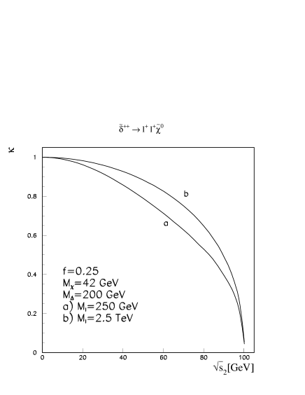
Figure 12: Values of the paramater $\kappa$ in the decays (47) and (50) as functions of the invariant mass of the final state $l^{+}l^{+}$ system for the masses indicated in the figure.

The paramater $\kappa$ in the decays (47) and (50) is shown in Fig.12 as a function of the invariant mass $\sqrt{s_{2}}$ of the final state $l^{+}l^{+}$ system. $\kappa$ is in general large over the whole range of the invariant mass and approaches zero only at the kinematical limit. If the virtual sleptons mediating the decay are very heavy (curve $b$ in Fig.12), the slepton propagators can be approximated by point propagators. In this case, the analytic expression for $\kappa$ in the $\tilde{\Delta}^{++}$ decay is particularly simple,

$$\kappa(s_{2})=\frac{\lambda\left[2(M_{\tilde{\Delta}^{++}}^{2}-m_{\tilde{\chi}^{0}}^{2})-s_{2}\right]}{\lambda^{2}+3s_{2}(M_{\tilde{\Delta}^{++}}^{2}+m_{\tilde{\chi}^{0}}^{2})-3(M_{\tilde{\Delta}^{++}}^{2}-m_{\tilde{\chi}^{0}}^{2})^{2}}$$ (62)

where $\lambda=[M_{\tilde{\Delta}^{++}}^{2}-(\sqrt{s_{2}}-m_{\tilde{\chi}^{0}}^{2})^{2}]^{1/2}[M_{\tilde{\Delta}^{++}}^{2}-(\sqrt{s_{2}}+m_{\tilde{\chi}^{0}}^{2})^{2}]^{1/2}.$ For the decay (50) of $\tilde{\delta}^{++}$ the parameter $\kappa$ has the opposite sign but the absolute value is numerically equal to the $\tilde{\Delta}^{++}$ decay.

4.2 Angular Correlations

The two–fold ambiguity in extracting the $\tilde{\Delta}^{++}$ and $\tilde{\delta}^{++}$ couplings from the total cross sections can be resolved by measurements of angular correlations which reflect the polarization states of the higgsinos in the production processes:

The analyses are complicated since the two invisible neutralinos in the final state do not allow for a complete reconstruction of the events. In particular, it is not possible to measure the $\tilde{\Delta}^{++},\tilde{\delta}^{++}$ production angle $\Theta$; this angle can be determined only up to a two–fold ambiguity which, however, becomes increasingly less effective with rising energy.

The final state distributions can be found by combining the polarized cross section with the polarized decay distributions. After integrating over the unobservable production angle $\Theta$ and the $(l^{+}l^{+})$ and $(l^{-}l^{-})$ invariant masses, the integrated cross section

$$\frac{{\rm d}^{4}\sigma\left[e^{+}e^{-}\rightarrow\tilde{\Delta}^{++}\tilde{\Delta}^{--}\rightarrow\tilde{\chi}^{0}_{1}\tilde{\chi}^{0}_{1}(l^{+}l^{+})(l^{-}l^{-})\right]}{{\rm d}\cos\theta^{*}{\rm d}\phi^{*}{\rm d}\cos\bar{\theta}^{*}{\rm d}\bar{\phi}^{*}}\hskip 28.45274pt$$

$$\hskip 11.38092pt=\frac{\alpha^{2}\beta}{128\pi s}{\rm Br}(\tilde{\Delta}^{++}\rightarrow\tilde{\chi}^{0}_{1}l^{+}l^{+}){\rm Br}(\tilde{\Delta}^{--}\rightarrow\tilde{\chi}^{0}_{1}l^{-}l^{-})\Sigma(\theta^{*},\phi^{*};\bar{\theta}^{*},\bar{\phi}^{*})\;\;\;\;\;\;\;\;\;\;\;\;\;\;\;\;\;\;\;\;\;$$ (63)

can be decomposed into sixteen independent angular parts. In addition to the unpolarized cross section, four angular distributions can be determined experimentally even though two neutralinos escape undetected:

$$\Sigma = \Sigma_{\rm unpol}+\cos\theta^{*}\kappa{\cal P}+\cos\bar{\theta}^{*}\bar{\kappa}\bar{\cal P}+\cos\theta^{*}\cos\bar{\theta}^{*}\kappa\bar{\kappa}{\cal Q}$$ (64)

$$+\sin\theta^{*}\sin\bar{\theta}^{*}\cos(\phi^{*}+\bar{\phi}^{*})\kappa\bar{\kappa}{\cal Y}+.....$$

The ellipsis denotes the remaining orthogonal angular distributions which cannot be measured. The polarizations ${\cal P}$ and $\bar{\cal P}=-{\cal P}$ have been expressed in terms of the generalized charges in eq.(34). Analogously,

Figure 13: Correlation functions ${\cal P},$ ${\cal Q}$ and ${\cal Y}$ normalized to $\Sigma_{\rm unpol}$ as functions of the collision energy for the processes $e^{+}e^{-}\rightarrow\tilde{\Delta}^{++}\tilde{\Delta}^{--}$ and $e^{+}e^{-}\rightarrow\tilde{\delta}^{++}\tilde{\delta}^{--}$.

the correlation functions ${\cal Q}$ and ${\cal Y}$ are defined by the charges in the following way:

$${\cal Q}=-4\int{\rm d}\cos\Theta\left[(\beta^{2}+\cos^{2}\Theta)Q_{1}+(1-\beta^{2})\cos^{2}\Theta Q_{2}+2\beta\cos\Theta Q_{3}\right]$$

$${\cal Y}=-2\int{\rm d}\cos\Theta(1-\beta^{2})\left[Q_{1}+Q_{2}\right]\sin^{2}\Theta$$ (65)

The energy dependence of the three correlation functions, ${\cal P},$ ${\cal Q}$ and ${\cal Y,}$ normalized to $\Sigma_{\rm unpol}$ is shown in Fig.13. For the both processes $e^{+}e^{-}\rightarrow\tilde{\Delta}^{++}\tilde{\Delta}^{--}$ and $e^{+}e^{-}\rightarrow\tilde{\delta}^{++}\tilde{\delta}^{--}$ they are smooth functions of the c.m. energy, quite different from zero for all values of the energy.

5. Observables of the Doubly Charged Higgsinos

5.1 Signals and Background

The final states of the doubly charged higgsino pair production processes (1), (2) and their subsequent decays (42), (44) or (47), (50) consist of four charged leptons $l_{1}^{+}l_{1}^{+}l_{2}^{-}l_{2}^{-}$ plus missing energy $\not\!\!E$. Because $\tilde{\Delta}^{++}$, $\tilde{\delta}^{++}$ carry two units of lepton number and two units of electric charge, the final state leptons with the same charge and flavor are associated with the same decaying particle:

$$e^{+}e^{-} \rightarrow \tilde{\Delta}^{++}\tilde{\Delta}^{--},\;\tilde{\delta}^{++}\tilde{\delta}^{--}$$ (66)

$$\rightarrow (l^{+}l^{+})(l^{-}l^{-})+\!\!\not\!\!E$$

The final–state observables of the signals are therefore clearly distinct from the background processes in which same–sign dileptons originate necessarily from decays of different particles.

Indeed, the main SM background is due to triple gauge–boson production: $e^{+}e^{-}\rightarrow\gamma^{*}W^{+}W^{-}\rightarrow l^{+}l^{-}l^{+}l^{-}+\!\!\not\!\!E$ etc. These processes are of higher order in the gauge couplings so that the cross sections are small and the backgrounds are under control. SUSY–induced backgrounds are generated by the production of heavy neutralinos that can decay into $\tilde{\chi}^{0}_{1}$ and a charged lepton pair: $e^{+}e^{-}\rightarrow\tilde{\chi}^{0}_{i}\tilde{\chi}^{0}_{j}\rightarrow l^{+}l^{-}l^{+}l^{-}+\!\!\not\!\!E$. Since, in both cases, the kinematical configurations of the background and signal events are very different from each other, the large number of events can be used to enrich the sample of signal events statistically by applying suitable cuts to disentangle signal from background effects.

Mass. The masses $M_{\tilde{\Delta}^{++}}$ and $M_{\tilde{\delta}^{++}}$ can be measured very precisely near the thresholds where the production cross sections $\sigma(e^{+}e^{-}\rightarrow\tilde{\Delta}^{++}\tilde{\Delta}^{--}/\tilde{\delta}^{++}\tilde{\delta}^{--})$ rise sharply with the velocities $\beta=\sqrt{1-4M^{2}_{\tilde{\Delta}^{++}}/s}$ and $\sqrt{1-4M^{2}_{\tilde{\delta}^{++}}/s}$, respectively. With beam parameters as anticipated for TESLA, a precision better than $\sim$ 100 MeV can be achieved by this method for an integrated luminosity of 50 fb^-1 [25].

Isospin. As evident from eq.(18), the isospin of the two states $\tilde{\Delta}^{++}$ and $\tilde{\delta}^{++}$ can be measured by using right– and left–handedly polarized electron beams. The two cross sections depend quadratically on the isospin,

$$\sigma(e^{+}e^{-}\rightarrow\tilde{\Delta}^{++}\tilde{\Delta}^{--})=\frac{4\pi\alpha^{2}}{s}\beta\left[\,1+c(s)I_{3}\,\right]^{2}$$ (67)

yet the root ambiguity can easily be resolved by carrying out the measurements at two different beam energies. The vector–character of the states can be proven by establishing the vanishing of forward–backward asymmetries.

Trilinear couplings $f$. Once the isospin components are determined, the couplings $f_{\tilde{\Delta}}$ and $f_{\tilde{\delta}}$ can be probed by measuring the cross sections in the mirror processes for right– and left–handedly polarized electron beams, respectively, cf. eqs.(25,26). The selectron masses are assumed to be known from the pair production of these particles. The measurements of the cross sections lead, in general, to a two–fold ambiguity in $f$. This ambiguity can be resolved in two ways. (i) If large enough variations in the cm energy are possible, measurements at two different energy points give rise to two independent equations for $f$ with only one common solution for both. (ii) The ambiguity can also be resolved by analyzing spin correlations. Since two invisible neutralinos are present in the final states after the decays of $\tilde{\Delta}$ and $\tilde{\delta}$, the kinematics of the $\tilde{\Delta}$ and $\tilde{\delta}$ states cannot be reconstructed completely. Nevertheless, the polar angles $\vartheta_{*}$ and the product of the transverse momentum vectors of the two $\tilde{\chi}^{0}_{1}$’s can be expressed by measured energies and laboratory angles,

$$\cos\theta^{*}=\frac{1}{\beta|\vec{p}^{*}|}\left(\frac{E}{\gamma}-E^{*}\right)\ \ {\rm and}\ \ \cos\bar{\theta}^{*}=\frac{1}{\beta|\vec{\bar{p}}^{*}|}\left(\frac{\bar{E}}{\gamma}-\bar{E}^{*}\right)$$

$$\sin\theta^{*}\sin\bar{\theta}^{*}\cos(\phi^{*}+\bar{\phi}^{*})=\frac{|\vec{p}||\vec{\bar{p}}|\cos\vartheta+\left(E-E^{*}/\gamma\right)\left(\bar{E}-\bar{E}^{*}/\gamma\right)}{\beta^{2}|\vec{p}^{*}||\vec{\bar{p}}^{*}|}$$ (68)

where $\gamma=\sqrt{s}/{2M_{\tilde{\Delta}^{++}}}$ etc.; $\vartheta$ is the angle between the momenta of the two lepton systems with opposite charges. As evident from eq.(64), the degree of polarizations ${\cal P}$ and $\bar{\cal P}$, and the spin correlations ${\cal Q}$ and ${\cal Y}$ can be measured directly despite the two neutralinos escaping detection.

The correlation functions come with the spin analysis–powers $\kappa$ and $\bar{\kappa}$ which depend on masses and couplings involving the neutralinos $\tilde{\chi}^{0}_{1}$. The $\kappa,\bar{\kappa}$ dependence however factorizes out of the correlation functions so that these parameters can be eliminated by taking appropriate ratios. As a result, two independent observables can be constructed from angular correlations, which can be measured directly in terms of laboratory momenta: ${\cal P}^{2}/{\cal Q}$ and ${\cal Y}/{\cal Q}$.

Figure 14: Contour lines from the measurements of $\sigma,$ ${\cal P}^{2}/{\cal Q}$ and ${\cal Y}/{\cal Q}$ determining the couplings $f$ and the weak isospin $I_{3}$ of the doubly charged higgsinos $\tilde{\Delta}^{++}$ and $\tilde{\delta}^{++}$. The common crossing point is indicated by the dot.

To demonstrate that the ambiguity can be resolved by measuring the spin correlations, we assume, in a Gedanken–experiment, a set of “measured observables”, i.e.unpolarized cross sections and correlation ratios; for illustration:

$\tilde{\Delta}^{++}$ :	$\sigma$ = 0.139 pb	${\cal P}^{2}/{\cal Q}$ = -2.81	${\cal Y}/{\cal Q}$ = 0.27
$\tilde{\delta}^{++}$ :	$\sigma$ = 0.093 pb	${\cal P}^{2}/{\cal Q}$ = -2.12	${\cal Y}/{\cal Q}$ = 0.23

The contour lines of these observables are shown in Figs.14 in the planes [$I_{3},f$], assuming the collision energy to be $\sqrt{s}=500$ GeV and higgsino and selectron masses $200$ GeV and 250 GeV, respectively. While the contours of $\sigma,{\cal P}^{2}/{\cal Q},{\cal Y}/{\cal Q}$ give pairwise rise to several intersections, the curves cross each other, all at the same time, only once. Moreover, this crossing point is the only solution that is consistent with integer/half–integer values of $I_{3}$, i.e. $I_{3}(\tilde{\Delta}^{++})=+1$ and $I_{3}(\tilde{\delta}^{++})=0$. Thus a unique solution for quantum numbers and couplings can be extracted from the measurements of (un)polarized cross sections, forward–backward asymmetries, and spin–spin correlations.

In the case of sufficiently light doubly charged higgsinos and relatively heavy selectrons, the cross sections and spin correlations can be exploited to determine the selectron masses. If the selectrons are too heavy to be pair produced, their masses can be estimated from their virtual contributions to the higgsino production processes. This is demonstrated for the “measured values” given above by the [$f,M_{\tilde{e}}$] contours in Figs.15. In these examples, the isospin quantum numbers are assumed to be pre–fixed in polarized–beam measurements.

Figure 15: Contour lines from the measurements of $\sigma,$ ${\cal P}^{2}/{\cal Q}$ and ${\cal Y}/{\cal Q}$ in the processes $e^{+}e^{-}\rightarrow\tilde{\Delta}^{++}\tilde{\Delta}^{--}$ and $e^{+}e^{-}\rightarrow\tilde{\delta}^{++}\tilde{\delta}^{--}.$ The common crossing point is indicated by the dot.

Acknowledgments

We are grateful to S. Ambrosanio, S.-Y. Choi, U. Sarkar, G. Senjanović, M. Spira and F. Vissani for helpful discussions and K. Huitu for useful comments. M.R. thanks the Humboldt Foundation for a grant and Prof. A. Wagner for the warm hospitality extended to him at DESY.

References

- [1] For recent reviews see, e.g., M. Takita, J. Conrad, M. Spiro, E. Kolb and R. Peccei, Proceedings ICHEP98, Vancouver 1998.
- [2] J.C. Pati and A. Salam, Phys. Rev. D10 (1974) 275: R.N. Mohapatra and J.C. Pati, Phys. Rev. D11 (1975) 566, 2558; G. Senjanović and R.N. Mohapatra, Phys. Rev. D12 (1975) 1502.
- [3] H. Fritzsch and P. Minkowski, Ann. Phys. 93 (1975) 193.
- [4] For a review, see J. Hewett and T. Rizzo, Phys. Rep. 183 (1989) 193.
- [5] C.S. Aulakh, K. Benakli and G. Senjanović, Phys. Rev. Lett. 79 (1997) 2188; C.S. Aulakh, A. Melfo and G. Senjanović, Phys. Rev. D57 (1998) 4174; Z. Chacko and R.N. Mohapatra, Phys. Rev. D58 (1998) 5001.
- [6] C.S. Aulakh, A. Melfo, A. Raśin and G. Senjanović, hep-ph/9712551.
- [7] Z. Chacko and R.N. Mohapatra, hep-ph/9802388.
- [8] M. Gell-Mann, P. Ramon and R. Slansky, in Supergravity, ed. P. van Niewenhuizen and D. Freedman (North-Holland, Amsterdam, 1979); T. Yanagida, in Proceedings of the Workshop on the Unified Theory and the Baryon Number in the Universe, ed. O. Sawada and A. Sugamoto (Tsukuba, 1979); R.N. Mohapatra and G. Senjanović, Phys. Rev. Lett. 44 (1980) 912.
- [9] K. Huitu, J. Maalampi and M. Raidal, Nucl. Phys. B420 (1994) 449, Phys. Lett. B328 (1994) 60.
- [10] B. Dutta and R.N. Mohapatra, hep-ph/9804277.
- [11] T. Rizzo, Phys. Rev. D25 (1982) 1355, Phys. Rev. D27 (1983) 657; M. Lusignoli and S. Petrarca, Phys. Lett. B226 (1989) 397; M.D. Swartz, Phys. Rev. D40 (1989) 1521; J.A. Grifols, A. Mendez and G.A. Schuler, Mod. Phys. Lett. A4 (1989) 1485; J.F. Gunion, J.A. Grifols, A. Mendez, B. Kayser and F. Olness, Phys. Rev. D40 (1989) 1546; J. Maalampi, A. Pietilä and M. Raidal, Phys. Rev. D48 (1993) 4467; N. Lepore et al., Phys. Rev. D50 (1994) 2031; E. Accomando and S. Petrarca, Phys. Lett. B323 (1994) 212; J.F. Gunion, Int. J. Mod. Phys. A11 (1996) 1551; J.F. Gunion, C. Loomis and K.T. Pitts, hep-ph/9610327; K. Huitu, J. Maalampi, A. Pietilä and M. Raidal, Nucl. Phys. B487 (1997) 27; G. Barenboim, K. Huitu, J. Maalampi and M. Raidal, Phys. Lett. B394 (1997) 132; F. Cuypers and M. Raidal, Nucl. Phys. B501 (1997) 3; M. Raidal, Phys. Rev. D57 (1998) 2013; S. Chakrabarti, D. Choudhuri, R.M. Godbole and B. Mukhopadhyaya, hep-ph/9804297.
- [12] S.-Y. Choi, A. Djouadi, H. Dreiner, J. Kalinowski and P.M. Zerwas, DESY 98-007 [hep-ph/9806279], Eur. Phys. J. C in press.
- [13] R. Kuchimanchi, Phys. Rev. Lett. 76 (1996) 3486; R.N. Mohapatra and A. Rasin, Phys. Rev. Lett. 76 (1996) 3490; R.N. Mohapatra, A. Rasin and G. Senjanović, Phys. Rev. Lett. 79 (1997) 4744. For a review see, e.g., R.N. Mohapatra, hep-ph/9801235.
- [14] For the early studies of SUSY left-right models, see M. Cvetic and J. Pati, Phys. Lett. B135 (1984) 57; Y. Ahn, Phys. Lett. B149 (1984) 337; R.M. Francis, M. Frank and C.S. Kalman, Phys. Rev. D43 (1991) 2369; R.M. Francis, C.S. Kalman and H.N. Saif, Z. Phys. C59 (1993) 655; K. Huitu, J. Maalampi and M. Raidal, Ref.[9].
- [15] R. Kuchimanchi and R.N. Mohapatra, Phys. Rev. D48 (1993) 4352; Phys. Rev. Lett. 75 (1995) 3989; K. Huitu and J. Maalampi, Phys. Lett. B344 (1995) 217.
- [16] K. Huitu, J. Maalampi and K. Puolamäki, hep-ph/9705406 and hep-ph/9708491.
- [17] C. Aulakh and R.N. Mohapatra, Phys. Rev. D28 (1983) 217; J. Maalampi amd J. Pulido, Nucl. Phys. B228 (1983) 242.
- [18] G. Beall, M. Bander and A. Soni, Phys. Rev. Lett. 48, (1982) 848; G. Barenboim, J. Bernabéu, J. Prades and M. Raidal, Phys. Rev. D 55, (1997) 4213.
- [19] For reviews of supersymmetry and the Minimal Supersymmetric Standard Model, see H. Nilles, Phys. Rep. 110 (1984) 1; H.E. Haber and G.L. Kane, Phys. Rep. 117 (1985) 75.
- [20] M. Raidal and A. Santamaria, Phys. Lett. B421 (1998) 250; and references therein.
- [21] H. Georgi, H. Quinn and S. Weinberg, Phys. Rev. Lett. 33 (1974) 451.
- [22] B. Brahmachari, U. Sarkar and K. Sridhar, Phys. Lett. B297 (1992) 105.
- [23] L.M. Sehgal and P.M. Zerwas, Nucl. Phys. B183 (1981) 417.
- [24] L. Michel and A.S. Wightman, Phys. Rev. 98 (1955) 1190; C. Bouchiat and L. Michel, Nucl. Phys. 5 (1958) 416; S.Y. Choi, Taeyeon Lee and H.S. Song, Phys. Rev. D40 (1989) 2477.
- [25] E. Accomando et al., Phys. Rep. 299 (1998) 1.
- [26] I. Ginzburg, G. Kotkin, V. Serbo and V. Telnov, Nucl. Inst. Methods 205 (1983) 47.
- [27] I. Watanabe et al., Report KEK-REPORT-97-17.
- [28] B. Dutta, R.N. Mohapatra and D.J. Muller, hep-ph/9810443.
- [29] G. Moortgat-Pick and H. Fraas, Report WUE-ITP-97-026 [hep-ph/9708481]; G. Moortgat-Pick, H. Fraas, A. Bartland, and W. Majerotto, Report WUE-ITP-98-012 [hep-ph/9804306].