Inherent Biases in the Ansatz Function Method used to Search for New Particles Decaying to Two-Jets in $\bar{p}p$ Collisions.

Abstract

Searches for new resonant phenomena on top of a continuum spectra need to make assumptions regarding the shape of the continuum spectra. The Ansatz function method used in previous searches for new particles decaying to dijets is investigated and found to have inherent biases that cause the 95$\%$ confidence limits on the signal cross-section to be miss-measured by up to 30 to 50$\%$.

Previous searches for hypothetical particles produced in proton–anti-proton collisions which decay to two-jets [1, 2, 3, 4] have utilized a procedure where the QCD inclusive two-jet mass spectrum is fitted as a linear combination of an ansatz function and a signal line shape to determine limits on the production cross section for various theoretical particles. The reliability of this procedure depends on the ability of the ansatz function to correctly model the mass spectrum of the continuum background. This paper describes a test of this procedure.

For this test the QCD inclusive two-jet mass spectrum resulting from $\bar{p}p$ collisions at $\sqrt{s}=1.8$ TeV was simulated using the Next–to–leading order (NLO) event generator jetrad [5] and the CTEQ4M [6] parton distribution function (pdf), a renormalization scale ($\mu$) of $0.5\mbox{$E_{T}^{\rm max}$}$ where $E_{T}^{\rm max}$ is the maximum jet transverse energy ($E_{T}$) of the event and a parton clustering algorithm. For the clustering algorithm, all partons within $1.3{\cal R}$ (${\cal R}=\sqrt{\eta^{2}+\phi^{2}}$) of one another were combined if they were also within ${\cal R}=0.7$ of their $E_{T}$ weighted $\eta$,$\phi$ centroid [7] where $\eta=-{\rm ln}[{\rm tan}(\theta/2)]$, $\theta$ is the polar angle relative to the proton beam and $\phi$ is the azimuthal angle. The $E_{T}$ of the jets are then smeared using typical collider jet resolutions [8]. The two-jet mass for each event was calculated using the two highest $E_{T}$ jets assuming that the jets are massless, using the relationship; $M^{2}=2\mbox{$E_{T}^{{\rm jet}1}$}\mbox{$E_{T}^{{\rm jet}2}$}[\cosh(\Delta\eta)-\cos(\Delta\phi)]$. The two leading $E_{T}$ were required to satisfy the requirements $\mbox{$\mid\!\eta_{\rm jet}\!\mid$}<1.0$, $\Delta\eta=\mid\!\eta_{1}-\eta_{2}\!\mid<1.6$, and $\mbox{$M$}>200$ GeV/c². The effects of statistical fluctuations in the prediction were removed by fitting to an ansatz function with the form:

$$A\cdot M^{-\alpha}\exp{\left[1-\left(\frac{M}{1800}\right)-\gamma\left(\frac{M}{1800}\right)^{2}-\delta\left(\frac{M}{1800}\right)^{3}\right]^{\beta}{\mathcal{P}}_{n}\left(\mbox{$M$}\right)}$$ (1)

where ${\mathcal{P}}_{n}\left(\mbox{$M$}\right)$ is a polynomial of degree $n$. The DØ Collaboration has demonstrated [9] that this simulation is a good representation of its measured Dijet Mass Spectrum.

To correctly model the statistical fluctuations typical of collider data samples, one hundred mass spectra were generated in 10 GeV/c² mass bins by smearing the spectrum obtained above with the Poisson fluctuations expected for the cross-section given by the simulation per bin times the luminosity for that bin. Four different mass regions, each with a different luminosity, were used to mimic data taking conditions, 0.5 pb^-1 for $200<\mbox{$M$}\leq 270$ GeV/c²; 5. pb^-1 for $270<\mbox{$M$}\leq 370$ GeV/c²; 50. pb^-1 for $370<\mbox{$M$}\leq 500$ GeV/c²; and 100. pb^-1 for $\mbox{$M$}>500$ GeV/c² . An example of one of the randomly generated spectra and the source distribution are shown in Fig. 1.

Three different ansatz functions will be investigated. The first is

$$F_{i}=\int_{M_{\mbox{\rm min}}}^{M_{\mbox{\rm max}}}A\left({\mbox{$M$}\over 100}\right)^{-\alpha}\left(1-{\mbox{$M$}\over 1800}\right)^{-\beta}d\mbox{$M$}.$$ (2)

where A is the normalization parameter and $\alpha$ and $\beta$ are fit parameters. Two additional ansatz functions were investigated. The first (equation 3) was used by the CDF collaboration [4] and the second (equation 5) by the UA2 collaboration [1, 2]:

$$F_{i} = \int_{M_{\mbox{\rm min}}}^{M_{\mbox{\rm max}}}A\left({\mbox{$M$}\over 100}\right)^{-\alpha}\left[1-{\mbox{$M$}\over 1800}+\gamma\left({\mbox{$M$}\over 1800}\right)^{2}\right]^{-\beta}d\mbox{$M$},$$ (3)

$$F_{i} = \int_{M_{\mbox{\rm min}}}^{M_{\mbox{\rm max}}}A\left({\mbox{$M$}\over 100}\right)^{-\alpha}\exp{\left[-\beta\left({\mbox{$M$}\over 100}\right)-\gamma\left({\mbox{$M$}\over 100}\right)^{2}\right]}d\mbox{$M$}.$$ (5)

The ansatz functions were all fitted to the 100 simulated spectra using a binned maximum likelihood method and the minuit [10] package. The resulting average $\chi^{2}$ for the fits is 59 for 52 data bins. The residuals ([data - fit]/fit) for each of the fits are depicted in Fig. 2. These residuals show that the ansatz functions do represent the mass spectra well with no obvious biases.

The 100 simulated spectra were then fitted with a linear combination of the ansatz function and a signal line shape,

$$F_{i}=\left[\int_{M_{\mbox{\rm min}}}^{M_{\mbox{\rm max}}}A\left({\mbox{$M$}\over 100}\right)^{-\alpha}\left(1-{\mbox{$M$}\over 1800}\right)^{-\beta}d\mbox{$M$}\right]+N_{X}S_{i}(M_{\mbox{$q^{\ast}$}}).$$ (6)

where $N_{\rm X}$ is the number of signal events expected from a hypothetical particle for the total luminosity and $S_{i}(\mbox{$q^{\ast}$})$ is the fraction of signal events in a given mass bin $i$ for a given signal mass. For this analysis the signal line shape is given by that of an excited quark ($q^{\ast}$) [11] which decays to a quark and a gluon ($\mbox{$q^{\ast}$}\rightarrow qg$). The coupling parameters of the excited quark theory were set equal to one ($f=f^{\prime}=f_{s}=1.0$) and the compositeness scale was set equal to the mass of the excited quark ($\Lambda^{\ast}=M_{\mbox{$q^{\ast}$}}$). The $q^{\ast}$ were simulated with masses from 200 to 975 GeV/² at 25 GeV/c² intervals using the pythia [12] event generator. The resulting particle jets were smeared with the assumed jet resolutions. Each $q^{\ast}$ sample contains fifty thousand events . Examples of $q^{\ast}$ mass spectra are shown in Fig 1.

For each of the one hundred background spectra the signal size $N_{\rm X}$ and its error $\Delta N_{\rm X}$ was determined for each of the $q^{\ast}$ masses generated. The average values of $N_{\rm X}$ ($\overline{N_{\rm X}}$) and $\Delta N_{\rm X}$ ($\overline{\Delta N_{\rm X}}$) were then calculated by fitting the distribution of $N_{\rm X}$ values obtained from the 100 spectra to a Gaussian distribution (see Fig. 3). $\overline{N_{\rm X}}$ is given by the central value of the Gaussian and $\overline{\Delta N_{\rm X}}$ is given by the width of the Gaussian.

The 95$\%$ confidence limit (CL) on the excited quark production cross section was then determined by assuming that the probability density as a function of cross section is given by a Gaussian with a center $\overline{N_{\rm X}}/{\cal{L}}$ and width $\overline{\Delta N_{\rm X}}/{\cal{L}}$. The $95\%$ CL on the cross section ($\sigma_{\mbox{\rm 95\%}}$) is then given by the value of the cross section such that $95\%$ of the physical part (i.e. the cross section is greater than zero) of the probability density function is below this value.

Since the spectra being fitted are derived from a NLO QCD calculation, the value of $\overline{N_{\rm X}}$ should be consistent with zero. Any deviation is the result of an inherent bias in the ansatz method. Figure 4 shows the fitted $\overline{N_{\rm X}}$ versus dijet mass. The error on $\overline{N_{\rm X}}$ is taken to be $\overline{\Delta N_{\rm X}}/\sqrt{99}$, and it is clear that there are systematic biases in the value of $\overline{N_{\rm X}}$ as a function of signal ($q^{\ast}$) mass.

If there were no bias in the ansatz fitting method the $95\%$ CL on the production cross section would be given by $1.96\times\overline{\Delta N_{\rm X}}$. A measure of the bias in the ansatz is the the difference between $\sigma_{\mbox{\rm 95\%}}$ and $1.96\times\overline{\Delta N_{\rm X}}$:

$$\mbox{Bias}={{\sigma_{\mbox{\rm 95\%}}-(1.96\times\overline{\Delta N_{\rm X}})}\over{1.96\times\overline{\Delta N_{\rm X}}}}$$ (7)

The resulting biases are given in Table I and are depicted in Figure 5 (solid circles). The plot clearly shows that the resulting $95\%$ CL on the production cross section can be miss-measured by up to $\pm 50\%$.

To see if these biases are caused by the specific choice of ansatz function, the two other possibilities were examined (equation 3 and 5). The bias values for these ansatz functions are given in Table II and are plotted in Fig. 5. It is clear that all three of the ansatz functions investigated produce a large bias in the resulting $95\%$ CL on the cross-section of up to 50$\%$. For a large range of mass values all of the ansatz functions produce biases of the same sign and approximate value and in some cases none of the limits will include the true 95$\%$ CL on the cross section. As limits are being set on new particle it is important to note that for a significant number of the mass values investigated the ansatz function method underestimates the $95\%$ CL.

The bias in the ansatz function method is caused by the changing slope of the dijet mass spectrum and the presence of a parameterized signal function. This signal function gives the ansatz function a flex point at which it can adapt to the changing slope of the data. The signal line shape fills a gap between the ansatz and the data producing a low $\chi^{2}$ fit. Therefore the requirement that the ansatz function fits the data with a small $\chi^{2}$ is not sufficient to show that the method is unbiased. It is also necessary to show that the method does not find a nonexistent signal.

The systematic uncertainties reported in previous searches [1, 2, 3, 4] are 50 to 300$\%$ depending on mass of the hypothetical particle. Hence, the limits reported by these searches will not be significantly degraded by this additional uncertainty. The bias in the method will prevent significant reduction of the systematic uncertainties in the future. The alternative to using an ansatz function to represent the background in these searches is a theoretical prediction (for example jetrad). Currently the uncertainties in these predictions are 30–40$\%$ [13] due to choice of renormalization scale and pdf. The effect of this uncertainty will have to be included in any future searches (this uncertainty can be reduced by improvements in the accuracy of pdf’s and theoretical calculations).

In conclusion it has been shown that the ansatz method of searching for new particles has an inherent bias in the method and this bias has to be accounted for when placing limits on the production cross-sections of new particle production.

I thank my colleagues on the DØ experiment for their helpful comments, suggestions and discussions. This work was supported in part by the Department of Energy under grant DE-FG02-91ER40684 at Northwestern University.

TABLE I.: The $95\%$ Confidence Limits obtained as a function of the mass of the $q^{\ast}$. Presented are the limits calculated from the fit using $\overline{N_{\rm X}}$ and $\overline{\Delta N_{\rm X}}$, the limit calculated using $1.96\times\overline{\Delta N_{\rm X}}$ and the bias.

$q^{\ast}$	Width		Fit		Bias	$q^{\ast}$	Width		Fit		Bias
Mass	Limit		Limit			Mass	Limit		Limit
	$1.96\times\overline{\Delta N_{\rm X}}$		$\sigma_{\mbox{\rm 95\%}}$				$1.96\times\overline{\Delta N_{\rm X}}$		$\sigma_{\mbox{\rm 95\%}}$
(GeV/c2)	($pb$)		($pb$)		($\%$)	(GeV/c2)	($pb$)		($pb$)		($\%$)
$200.$	$1.80$×10	2	$1.99$×10	2	$10.$	$225.$	$2.98$×10	2	$3.35$×10	2	$12.$
$250.$	$3.11$×10	2	$3.22$×10	2	$4.$	$275.$	$8.88$×10	1	$8.35$×10	1	$-6.$
$300.$	$7.64$×10	1	$6.82$×10	1	$-11.$	$325.$	$6.00$×10	1	$4.53$×10	1	$-24.$
$350.$	$4.73$×10	1	$3.85$×10	1	$-18.$	$375.$	$2.59$×10	1	$2.33$×10	1	$-10.$
$400.$	$1.38$×10	1	$1.11$×10	1	$-19.$	$425.$	$9.92$×10	0	$8.78$×10	0	$-12.$
$450.$	$9.27$×10	0	$8.82$×10	0	$-5.$	$475.$	$6.92$×10	0	$7.51$×10	0	$8.$
$500.$	$5.69$×10	0	$7.01$×10	0	$23.$	$525.$	$3.60$×10	0	$4.70$×10	0	$30.$
$550.$	$3.07$×10	0	$4.07$×10	0	$32.$	$575.$	$2.51$×10	0	$3.59$×10	0	$43.$
$600.$	$1.84$×10	0	$2.86$×10	0	$56.$	$625.$	$2.16$×10	0	$2.88$×10	0	$34.$
$650.$	$1.74$×10	0	$2.36$×10	0	$35.$	$675.$	$1.28$×10	0	$1.59$×10	0	$24.$
$700.$	$1.09$×10	0	$1.26$×10	0	$15.$	$725.$	$0.83$×10	0	$0.79$×10	0	$-5.$
$750.$	$0.76$×10	0	$0.51$×10	0	$-34.$	$775.$	$0.65$×10	0	$0.29$×10	0	$-55.$
$800.$	$0.47$×10	0	$0.17$×10	0	$-64.$	$825.$	$0.38$×10	0	$0.16$×10	0	$-57.$
$850.$	$0.41$×10	0	$0.26$×10	0	$-36.$	$875.$	$0.34$×10	0	$0.26$×10	0	$-25.$
$900.$	$0.30$×10	0	$0.25$×10	0	$-16.$	$925.$	$0.41$×10	0	$0.37$×10	0	$-10.$
$950.$	$0.24$×10	0	$0.22$×10	0	$-9.$	$975.$	$0.24$×10	0	$0.23$×10	0	$-5.$

TABLE II.: The Biases for all three ansatz functions investigated. (Equation 2, Equation 3 and Equation 5 )

$q^{\ast}$	Bias			$q^{\ast}$	Bias
Mass	Equation 2	Equation 3	Equation 5	Mass	Equation 2	Equation 3	Equation 5
(GeV/c2)	($\%$)	($\%$)	($\%$)	(GeV/c2)	($\%$)	($\%$)	($\%$)
$200.$	$10.$	$4.$	$-2.$	$225.$	$12.$	$44.$	$34.$
$250.$	$4.$	$47.$	$36.$	$275.$	$-6.$	$12.$	$24.$
$300.$	$-11.$	$-14.$	$-1.$	$325.$	$-24.$	$-19.$	$-6.$
$350.$	$-18.$	$-5.$	$5.$	$375.$	$-10.$	$21.$	$22.$
$400.$	$-19.$	$8.$	$12.$	$425.$	$-12.$	$-13.$	$-14.$
$450.$	$-5.$	$-24.$	$-30.$	$475.$	$8.$	$-17.$	$-24.$
$500.$	$23.$	$12.$	$-2.$	$525.$	$30.$	$35.$	$18.$
$550.$	$32.$	$36.$	$22.$	$575.$	$43.$	$29.$	$28.$
$600.$	$56.$	$30.$	$21.$	$625.$	$34.$	$16.$	$15.$
$650.$	$35.$	$8.$	$27.$	$675.$	$24.$	$-2.$	$18.$
$700.$	$15.$	$-10.$	$18.$	$725.$	$-5.$	$-25.$	$4.$
$750.$	$-34.$	$-28.$	$-4.$	$775.$	$-55.$	$-33.$	$-2.$
$800.$	$-64.$	$-32.$	$0.$	$825.$	$-57.$	$-37.$	$-11.$
$850.$	$-36.$	$-38.$	$-12.$	$875.$	$-25.$	$-35.$	$-9.$
$900.$	$-16.$	$-24.$	$-20.$	$925.$	$-10.$	$-14.$	$-16.$
$950.$	$-9.$	$4.$	$-18.$	$975.$	$-5.$	$13.$	$-17.$

FIG. 1.: The QCD Dijet Mass Spectrum produced by the jetrad program (solid line) and one of the randomly generated spectra (solid circles). Note: That the randomly generated spectra has been corrected so that all points have the same apparent luminosity. Also shown are the simulated $q^{\ast}$ at masses of 300, 500 and 700 GeV/c² (dash–dot lines).

FIG. 2.: The values of the residuals ([data - fit]/fit) for each of ansatz functions fitted to the data with no signal function. The solid circles (a) show the results of the fits using the ansatz of equation 2, the open squares (b) show the results for Equation 3, and the open triangles show the results for Equation 5.

FIG. 3.: The distribution of the values of $N_{\rm X}$ obtained when the 100 simulated mass spectra are fitted with the ansatz function (Equation 2) and a 500 GeV/² $q^{\ast}$.

FIG. 4.: The values of $\overline{N_{\rm X}}$ (solid circles), the uncertainty of $\overline{N_{\rm X}}$=$\overline{\Delta N_{\rm X}}/\sqrt{99}$ (solid error bars) and $\overline{\Delta N_{\rm X}}$ (dotted error bars) obtained from fitting the simulated dijet mass spectra with Equation 2.

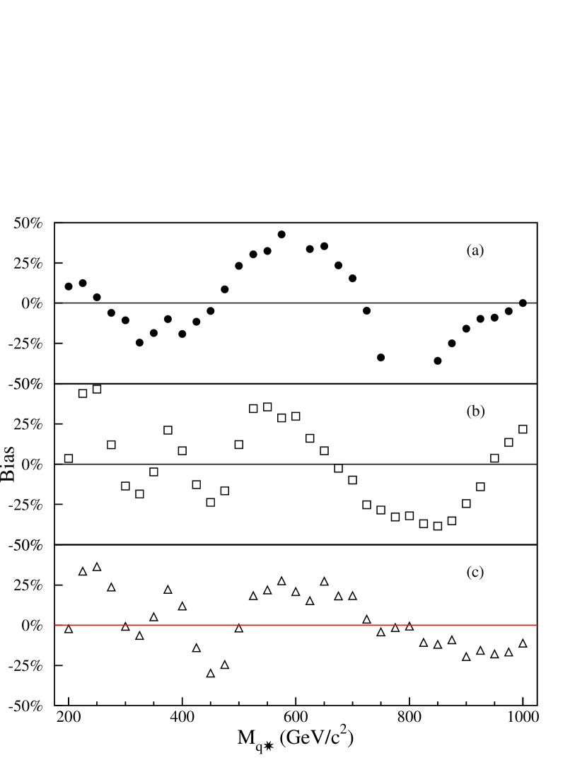
FIG. 5.: The Bias in the ansatz function method. The solid circles (a) show the bias due to ansatz of Equation 2, the open squares (b) show the bias due to the ansatz of Equation 3 and the open triangles (c) show the bias due to the ansatz of Equation 5.

REFERENCES

- [1] J. Alitti et al. (UA2 Collaboration), Zeit. Phys. C 49, 17 1991.
- [2] J. Alitti et al. (UA2 Collaboration), Nucl. Phys. B400, 3 (1993).
- [3] F. Abe et al. (CDF Collaboration), Phys. Rev. Lett. 74, 3538 (1995), hep-ex/9501001.
- [4] F. Abe et al. (CDF Collaboration), Phys. Rev. D 55, (1997), hep-ex/9702004.
- [5] W.T. Giele, E.W.N. Glover and D.A. Kosower, Nucl. Phys. B403, 633 (1993).
- [6] H.L. Lai et al., Phys. Rev. D 55, 1280 (1997), hep-ph/9606399.
- [7] B. Abbott et al. (for the DØ Collaboration), Fermilab-Pub-97/242-E.
- [8] M. Bhattacharjee, et al., DØ Internal Note 2887, Jet Energy Resolution, ( May 22, 1996)
- [9] B. Abbott et al. (DØ Collaboration), hep-ex/9807014, submitted to Phys. Rev. Lett.
-
[10]
F. James, CERN Program Library Entry D506 (unpublished),
http://wwwinfo.cern.ch/asdoc/minuit_html3/minmain.html.
minuit version 96.a was used. - [11] U. Baur, M. Spira and P.M. Zerwas, Phys. Rev. D 42, 815 (1990).
- [12] T. Sjöstrand, Computer Physics Commun. 82, 74 (1994). pythia version 5.7 was used.
- [13] B. Abbott, et al., hep-ph/9801285, Eur. Phys. J. C 5 687 (1998).