DTP/98/26

DESY/98/68

June 1998

Final state photon production at LEP
A. Gehrmann–De Ridder^a and E. W. N. Glover^{b a} DESY, Theory Group, D-22603 Hamburg, Germany

^b Department of Physics, University of Durham, Durham DH1 3LE, England

We present a detailed study of photon production in hadronic events in electron-positron annihilation at LEP energies. We show that estimates of the inclusive photon spectrum using the quark-to-photon fragmentation function determined using the ALEPH ‘photon’ + 1 jet data agree well with the observations of the OPAL collaboration. This agreement shows that the photon fragmentation function determined in this way can be used for inclusive observables. We also compare next-to-leading order and beyond leading logarithm predictions obtained using the numerically resummed solutions of the fragmentation function evolution equation of Bourhis, Fontannaz and Guillet and Glück, Reya and Vogt with the data. Moreover, in order to check the general behaviour of the fragmentation function, we consider an analytic series expansion in the strong coupling. We find that the parameterizations are inaccurate at large $x$ values. While the OPAL data is in broad agreement with estimates based on any of these approaches, the ALEPH data prefers the resummed BFG parameterization. Finally, there is some ambiguity as to whether the fragmentation function is treated as ${\cal O}(\alpha)$ or ${\cal O}(\alpha/\alpha_{s})$. We show that at present this ambiguity affects mainly the prediction for the ‘photon’ + 1 jet rate at large $z$.

1 Introduction

The production of hard photons in hadronic processes provides an important testing ground for QCD. For example, direct photon production in $p\bar{p}$ collisions is used to extract information on the gluon content of the proton, while the presence of photons in the final state represents an important background source in many searches for new physics. A good understanding of direct photon production within the context of the Standard model is therefore essential.

Photons produced in hadronic collisions can have two possible origins: the direct radiation of a photon off a primary quark and the fragmentation of a parton $i$ into a photon carrying a sizeable fraction $x$, of the parton energy. While the former direct process constitutes a short-distance effect and can be calculated within the framework of the Standard Model, the latter is primarily a long distance process. It is described by the process-independent parton-to-photon fragmentation function $D_{i\to\gamma}(x,\mu_{F})$, which cannot be calculated using perturbative methods but which must be determined from experimental data. The evolution of $D_{i\to\gamma}(x,\mu_{F})$ with the factorization scale $\mu_{F}$ can however be determined by perturbative QCD.

The most promising environment for a determination of the quark-to-photon fragmentation function $D_{q\to\gamma}(x,\mu_{F})$ is the study of photon production in electron-positron annihilation into hadrons. Such measurements have been recently presented by the ALEPH [1] and OPAL [2] collaborations at CERN. Both measurements differ not only in the experimental observable studied to determine the quark-to-photon fragmentation function, but also in the theoretical framework used to match direct and fragmentation contributions onto each other. This makes a comparison of both experiments difficult, and has also given rise to the speculation that the ALEPH and OPAL analyzes do not probe the same quantity [2, 3].

The analysis performed by ALEPH is based on the study of two jet events in which one of the jets contains a highly energetic photon. Correspondingly, the fraction of the jet momentum carried by the photon within the ‘photon’ jet, $z$, is greater than $0.7$. These events were defined by the application of the Durham jet clustering algorithm [4] to both hadronic and electromagnetic clusters. A comparison between the observed rate and the $\cal{\cal O}(\alpha)$ [1, 5] or ${\cal O}(\alpha\alpha_{s})$ [6] theoretical estimates yielded a first determination of the quark-to-photon fragmentation function accurate at leading and next-to-leading order. The theoretical basis on which the measurement of the ‘photon’ + 1 jet rate relies, is an explicit counting of powers of the strong coupling $\alpha_{s}$ in both the direct and the fragmentation contributions, and where no resummation of $\ln\mu_{F}^{2}$ is performed. We shall refer to this theoretical framework as the fixed order approach.

More recently, the OPAL collaboration has measured the inclusive photon distribution for final state photons with energies as small as 10 GeV. This corresponds to the photon carrying a fraction of the beam momentum, $x_{\gamma}$, to be as low as 0.2. They have compared their results with the model-dependent predictions of [3, 7] and found a reasonable agreement in both cases. These model predictions are based on a resummation of the logarithms of the factorization scale $\mu_{F}$ and naturally associate an inverse power of $\alpha_{s}$ with all fragmentation contributions. This resummation procedure is the conventional approach.

Although, the quark-to-photon fragmentation function is a purely non perturbative object, its evolution with the factorization scale can be described within perturbative QCD. In the fixed order approach, a byproduct of the perturbative calculation of the photon production cross section is an evolution equation which is accurate at a given order. This has been presented in some detail in [6], and we recall the main features in Section 2. In the conventional approach adopted by [3, 7] though, the quark-to-photon fragmentation function satisfies the well-known DGLAP [8] all order evolution equation and, as in the fixed order approach, this solution has a non-perturbative ingredient which can only be measured. We discuss the main steps in the formal derivation of this solution in the conventional formalism in Section 3.

A priori, it may indeed not be entirely clear that the fragmentation function extracted from a measurement of the ‘photon’ + 1 jet rate and the fragmentation function arising in the inclusive cross section are the same. In fact, the variables used in the definitions of these rates, $z$ for the photon rate and $x_{\gamma}$ for the inclusive rate are generally not equal to each other. As explained in Section 2, these variables coincide however in the purely ‘collinear’ region where the genuine non-perturbative effects arise so we can clarify this issue and affirm that these two fragmentation functions are indeed equal to each other. Information gained about the quark-to-photon fragmentation function from the analysis of one observable can (and ought to) be used to predict other photon cross sections.

So far the ALEPH collaboration have compared their data with the theoretical predictions obtained in a fixed order formalism while the OPAL collaboration have concentrated on the theoretical predictions from the conventional framework. However, because the fragmentation functions are universal, it is possible to evaluate the ‘photon’ + 1 jet rate and the inclusive rate obtained in either theoretical framework and to compare these predictions with either the ALEPH or the OPAL data. To perform such a comparison, and to see if the data prefers one approach, is the purpose of this paper.

More precisely the paper is organized as follows. In Section 2, we discuss how the quark-to-photon fragmentation function and the one-photon production cross section are determined in a fixed order approach and present the results obtained for the inclusive rate in this approach. In Section 3, we describe how the quark-to-photon fragmentation function is determined in a conventional approach. In particular we describe how the leading-logarithmic (LL) and beyond-leading logarithmic (BLL) solutions are determined and compare their numerical parameterizations with analytically expanded expressions of the quark-to-photon fragmentation function. Section 4 contains a detailed presentation of four possible different approaches to evaluate the one-photon production cross sections, one of these being closely related to the fixed order approach described in Section 2. The possible definitions of the non-perturbative input in either the schemes adopted by Glück, Reya and Vogt (GRV) in [7] or by Bourhis, Fontannaz and Guillet (BFG) in [3], are also discussed in this context. Moreover we study the behaviour of the parameterizations given in [3, 7] in the large $x$ region. In Section 5, we present results obtained following any of these four approaches and using either the GRV or BFG schemes for the inclusive and ‘photon’ + 1 jet cross sections and compare them with the OPAL and ALEPH data. Finally, Section 6 contains our conclusions.

2 Inclusive photon production in the fixed order approach

Let us first consider the general structure of the single photon production cross section, fully differential in all quantities,

$${\rm d}\sigma={\rm d}\hat{\sigma}_{\gamma}\;+\;\sum_{a}{\rm d}\hat{\sigma}_{a}\otimes D^{B}_{a\to\gamma}.$$ (2.1)

In this equation which is valid for any single photon production cross section there are two contributions. First ‘prompt’ photon production arises when the photon is produced directly in the hard interaction. Second, the longer distance fragmentation process occurs when one of the partons produced in the hard interaction fragments into a photon and transfers a fraction of the parent parton momentum to the photon. Each type of parton, $a$, contributes according to the process independent parton-to-photon fragmentation functions $D_{a\to\gamma}$ and the sum runs over all partons. At the order we are interested in, the gluon fragmentation functions will generally be small and can be neglected, as explained below. The sum therefore runs over all active quark and antiquark flavours. Moreover, by charge conjugation, quark and antiquark fragmentation functions are equal.

The individual terms in eq. (2.1) may be divergent and are denoted by hatted quantities. However, through the introduction of a factorization scale $\mu_{F}$, these terms can be reorganized and the physical cross section can be written in terms of finite (but factorization scale dependent) quantities,

$${\rm d}\sigma={\rm d}\sigma_{\gamma}(\mu_{F})\;+\;\sum_{a}{\rm d}\sigma_{a}\otimes D_{a\to\gamma}(\mu_{F}).$$ (2.2)

These two process specific contributions will be defined differently for the ‘photon’ + 1 jet and inclusive photon cross sections. Furthermore, as we shall see in Section 4 these will be defined differently depending which approach is used to evaluate these photon production cross sections.

We are primarily interested in the expression of the inclusive photon production evaluated at fixed order up to ${\cal O}(\alpha\alpha_{s})$. In this context, the hard cross sections as well as the non-perturbative fragmentation functions have to be considered at most up to ${\cal O}(\alpha\alpha_{s})$. Although the fragmentation functions are non-perturbative, we can nominally assign a power of coupling constants, based on counting the couplings necessary to radiate a photon. Since the photon couples directly to the quark, $D_{q\to\gamma}$ is naively of ${\cal O}(\alpha)$ while the gluon can only couple to the photon via a quark and $D_{g\to\gamma}$ can be considered to be of ${\cal O}(\alpha\alpha_{s})$. This simplistic argument is supported by models of the fragmentation function [3, 7] which suggest that gluon fragmentation is a much smaller effect than quark fragmentation. In $e^{+}e^{-}$ annihilation, the production of gluons is suppressed by a power of $\alpha_{s}$ compared to the production of quarks. As a result, the contribution from gluon fragmentation is of ${\cal O}(\alpha\alpha_{s}^{2})$ and should be neglected in a consistent evaluation of this rate at fixed order up to ${\cal O}(\alpha\alpha_{s})$.

In this fixed order approach the inclusive photon production cross section can be expressed as a function of the fraction of the beam energy carried by the photon $x_{\gamma}=2E_{\gamma}/\sqrt{s}$. At ${\cal O}(\alpha)$ it takes the following form,

$$\frac{1}{\sigma_{0}}\frac{{\rm d}\sigma^{LO}}{{\rm d}x_{\gamma}}=\sum_{q=1}^{2N_{F}}\;\left(\left(\frac{\alpha e_{q}^{2}}{2\pi}\right)C^{(0)}_{\gamma}(x_{\gamma},\mu_{F})\,+\;D_{q\to\gamma}(x_{\gamma},\mu_{F})\right),$$ (2.3)

while at ${\cal O}(\alpha\alpha_{s})$ it is given by,

$$\frac{1}{\sigma_{0}}\frac{{\rm d}\sigma^{NLO}}{{\rm d}x_{\gamma}}=\frac{1}{\sigma_{0}}\frac{{\rm d}\sigma^{LO}}{{\rm d}x_{\gamma}}+\left(\frac{\alpha_{s}}{2\pi}\right)\sum_{q=1}^{2N_{F}}\left(\left(\frac{\alpha e_{q}^{2}}{2\pi}\right)C^{(1)}_{\gamma}(x_{\gamma},\mu_{F})+C_{q}^{(0)}\otimes D_{q\to\gamma}(x_{\gamma},\mu_{F})\right).$$ (2.4)

Here, $\sigma_{0}$ is the two-particle cross section, $N_{F}$ stands for the number of flavours. We have moreover represented the convolution in a compact way,

$$\int^{1}_{x}\frac{dt}{t}A(t)B\left(\frac{x}{t}\right)=A\otimes B(x).$$ (2.5)

Figure 1: Parton level subprocesses contributing to single photon production at ${\cal O}(\alpha\alpha_{s})$.

The hard scattering coefficient functions $C_{i}^{(n)}$ appearing in these equations are defined as follows. $C^{(0)}_{\gamma}$ is the coefficient function corresponding to the lowest order process $e^{+}e^{-}\to q\bar{q}\gamma$. It is defined after the leading quark-photon singularity has been subtracted and factorized in the bare quark-to-photon fragmentation function. In the $\overline{MS}$ scheme it is given by [9],

$$C^{(0)}_{\gamma}(x_{\gamma},\mu_{F})=P^{(0)}_{q\to\gamma}(x_{\gamma})\,\ln\left(\frac{s(1-x_{\gamma})x_{\gamma}^{2}}{\mu_{F}^{2}}\right),$$ (2.6)

where $P^{(0)}_{q\to\gamma}(x)$ is the $\epsilon\to 0$ part of the the lowest order splitting function in $(4-2\epsilon)$-dimensions [8],

$$P_{q\to\gamma}(x)=\frac{1+(1-x)^{2}-\epsilon x^{2}}{x}.$$ (2.7)

The (finite) next-to-leading order coefficient function $C^{(1)}_{\gamma}$ can be obtained numerically after the next-to-leading quark-photon singularity has been subtracted. More precisely, $C^{(1)}_{\gamma}$ is obtained after summing all contributions which are independent of $D_{q\to\gamma}(x_{\gamma},\mu_{F})$ arising from the Feynman diagrams depicted in Fig. 1 together. A detailed description of the evaluation of $C^{(1)}_{\gamma}$ in the case of the ‘photon’ + 1 jet cross section has been given in [10]. The next-to-leading coefficient function appropriate for the inclusive photon production can moreover be straightforwardly obtained from the next-to-leading order coefficient function relevant for the ‘photon’ + 1 jet cross section by integrating the jet-specific variables over the complete phase space.

The coefficient function $C_{q}^{(0)}$ is the finite part associated with the sum of real and virtual gluon contributions to the process $e^{+}e^{-}\to q\bar{q}$. It is straightforward to evaluate, and can be found for example in [9],

$$C_{q}^{(0)}(x) = C_{F}\left[\left\{\frac{1+x^{2}}{(1-x)_{+}}+\frac{3}{2}\delta(1-x)\right\}\ln\left(\frac{s}{\mu_{F}^{2}}\right)\,+\,\left(\frac{2}{3}\pi^{2}-\frac{9}{2}\right)\delta(1-x)\right.$$ (2.8)

$$\left.+2\ln\left(x\frac{1+x^{2}}{1-x}\right)\,+\,(1+x^{2})\left(\frac{\ln(1-x)}{1-x}\right)_{+}-\frac{3}{2}\left(\frac{1}{1-x}\right)_{+}-\frac{3}{2}x+\frac{5}{2}\right],$$

where $C_{F}$ the Casimir operator is given by, $C_{F}=(N^{2}-1)/2N$. This color factor is also implicitly included in the next-to-leading order coefficient functions $C^{(1)}_{\gamma}$ defined above.

As motivated in [6], within the fixed order approach the process-independent quark-to-photon fragmentation function $D_{q\to\gamma}(x,\mu_{F})$ appearing in eq. (2.3) and eq. (2.4) respectively at leading and next-to-leading order, satisfies an exact (up to the order under consideration) evolution equation. At next-to-leading order (${\cal O}(\alpha\alpha_{s})$) this equation reads,

$$\frac{\partial D_{q\to\gamma}(x,\mu_{F})}{\partial\ln(\mu_{F}^{2})}=\left(\frac{\alpha e_{q}^{2}}{2\pi}\right)P^{(0)}_{q\to\gamma}(x)\,+\,\left(\frac{\alpha e_{q}^{2}}{2\pi}\right)\left(\frac{\alpha_{s}}{2\pi}\right)P^{(1)}_{q\to\gamma}(x)+\left(\frac{\alpha_{s}}{2\pi}\right)P^{(0)}_{q\to q}\otimes D_{q\to\gamma}(x,\mu_{F}).$$ (2.9)

$P^{(0)}_{q\to q}$ and $P^{(1)}_{q\to\gamma}$ are respectively the lowest order quark-to-quark and the next-to-leading order quark-to-photon universal splitting functions [8, 11, 12],

$$P^{(0)}_{q\to q}(x) = C_{F}\left[\frac{1+x^{2}}{(1-x)_{+}}+\frac{3}{2}\delta(1-x)\right],$$ (2.10)

$$P^{(1)}_{q\to\gamma}(x) = C_{F}\left[-\frac{1}{2}+\frac{9}{2}x+\left(-8+\frac{1}{2}x\right)\ln x+2x\ln(1-x)+\left(1-\frac{1}{2}x\right)\ln^{2}x\right.$$ (2.11)

$$\left.+\left(\ln^{2}(1-x)+4\ln x\ln(1-x)+8{\rm Li}_{2}(1-x)-\frac{4}{3}\pi^{2}\right)P^{(0)}_{q\to\gamma}(x)\right].$$

The quark-to-photon fragmentation function satisfying the evolution equation reads,

$$D_{q\to\gamma}^{(NLO)}(x,\mu_{F}) = D_{q\to\gamma}^{np}(x,\mu_{0})+\left(\frac{\alpha e_{q}^{2}}{2\pi}\right)\ln\left(\frac{\mu^{2}_{F}}{\mu_{0}^{2}}\right)P^{(0)}_{q\to\gamma}(x)$$ (2.12)

$$+ \left(\frac{\alpha e_{q}^{2}}{2\pi}\right)\left(\frac{\alpha_{s}}{2\pi}\right)\ln\left(\frac{\mu^{2}_{F}}{\mu_{0}^{2}}\right)P^{(1)}_{q\to\gamma}(x)$$

$$+ \frac{1}{2}\left(\frac{\alpha e_{q}^{2}}{2\pi}\right)\left(\frac{\alpha_{s}}{2\pi}\right)\ln^{2}\left(\frac{\mu^{2}_{F}}{\mu_{0}^{2}}\right)P^{(0)}_{q\to q}\otimes P^{(0)}_{q\to\gamma}(x)$$

$$+ \left(\frac{\alpha_{s}}{2\pi}\right)\ln\left(\frac{\mu^{2}_{F}}{\mu_{0}^{2}}\right)P^{(0)}_{q\to q}\otimes D_{q\to\gamma}^{np}(x,\mu_{0}).$$

This solution has some interesting properties. First, it is exact at the order of the calculation i.e. ${\cal O}(\alpha\alpha_{s})$, and yields no terms of higher orders. The inclusive rate with this solution implemented is therefore independent of the choice of the factorization scale $\mu_{F}$. The exact lowest order (${\cal O}(\alpha)$) evolution equation and its solution $D_{q\to\gamma}^{(LO)}(x,\mu_{F})$ are naturally contained in eq. (2.9) and eq. (2.12) respectively; they can be obtained by dropping all terms proportional to $\alpha_{s}$ in these equations.

In eq. (2.12), all a priori unknown non-perturbative contributions associated with the fragmentation function are contained in $D_{q\to\gamma}^{np}(x,\mu_{0})$ which has to be determined from the data. This non-perturbative input has been extracted from the ALEPH ‘photon’ + 1 jet data [1] for $y_{\rm cut}=0.06$ and $z>0.7$. At lowest order, we have [1],

$$D_{q\to\gamma}^{np(LO)}(x,\mu_{0})=\left(\frac{\alpha e_{q}^{2}}{2\pi}\right)\left(-P^{(0)}_{q\to\gamma}(x)\ln(1-x)^{2}-13.26\right),$$ (2.13)

with $\mu_{0}=0.14$ GeV while at next-to-leading order [6],

$$D_{q\to\gamma}^{np(NLO)}(x,\mu_{0})=\left(\frac{\alpha e_{q}^{2}}{2\pi}\right)\left(-P^{(0)}_{q\to\gamma}(x)\ln(1-x)^{2}\;+\,20.8\,(1-x)-11.07\right),$$ (2.14)

where $\mu_{0}=0.64$ GeV and for $\alpha_{s}(M_{Z})=0.124$.

However, in the ‘photon’ + 1 jet data, the process independent fragmentation function is extracted as a function of $z$, the fraction of the ‘photon’ jet momentum carried by the photon. This is in general different from the variable relevant for the inclusive rate which is $x_{\gamma}$, the fraction of the beam momentum carried by the photon. To see this, let us consider the lowest order process $e^{+}e^{-}\to q\bar{q}\gamma$, where the photon is emitted by the quark. For this process the two variables $x_{\gamma}$ and $z$ are defined as follows,

$$x_{\gamma}=\frac{2E_{\gamma}}{\sqrt{s}}=1-y_{q\bar{q}}=y_{q\gamma}+y_{\bar{q}\gamma},\hskip 28.45274ptz=\frac{E_{\gamma}}{E_{\gamma}+E_{q}}=\frac{y_{q\gamma}+y_{\bar{q}\gamma}}{1+y_{q\gamma}}$$ (2.15)

where $E_{\gamma}$ and $E_{q}$ are respectively the energies carried by the photon and the quark in the event and the dimensionless invariants $y_{ij}=(p_{i}+p_{j})^{2}/s$. Over most of phase space, the two variables are clearly different and results derived for the ‘photon’ + 1 jet cross section should in principle not be transferable to the inclusive rate. However, the non perturbative fragmentation effects are associated with the emission of a photon collinear to the quark and arise in the boundary region of the phase space where $y_{q\gamma}\to 0$. This is precisely where the definition of the two variables $z$ and $x_{\gamma}$ coincide. Furthermore, the collinear photon and quark region of the inclusive three parton phase space, is the same as the collinear phase space restricted to the ‘photon’ jet region, so that the contribution to the inclusive rate or to ‘photon’ + 1 jet rate from the collinear region is the same [3, 5],

$$\frac{1}{\sigma_{0}}\frac{{\rm d}\sigma^{col}}{{\rm d}x}=\left(\frac{\alpha e_{q}^{2}}{2\pi}\right)\left(P^{(0)}_{q\to\gamma}(x)\ln\left((1-x)x\right)+x\right)\equiv C_{\gamma}^{(col)}(x)$$ (2.16)

where $x$ can stand either for $x_{\gamma}$ or for $z$. As a consequence, the quark-to-photon fragmentation function obtained in the context of the calculation of the ‘photon’ + 1 jet rate is process independent, and can be used directly to estimate the inclusive photon rate. This statement is in contrast with claims made in the literature [2, 3].

Figure 2: The inclusive photon energy distribution normalized to the hadronic cross section as measured by the OPAL collaboration compared with the LO (${\cal O}(\alpha)$) and NLO (${\cal O}(\alpha\alpha_{s})$) calculations including the quark-to-photon fragmentation function determined at the appropriate order from the ALEPH ‘photon’ + 1 jet data.

We therefore show our predictions for the inclusive photon energy distribution at both ${\cal O}(\alpha)$ and ${\cal O}(\alpha\alpha_{s})$ in Fig. 2 using the fragmentation function extracted from the ‘photon’ + 1 jet data. For comparison we also show the measurements of the OPAL Collaboration [2]. We note that OPAL was able to identify photons with energies as little as 10 GeV, corresponding to $x_{\gamma}>0.2$. We see good agreement with the data for both the leading and next-to-leading order theoretical predictions. It is also apparent that the next-to-leading order corrections to the inclusive rate are of reasonable size indicating that the results obtained following this fixed order approach are perturbatively stable. The agreement between our predictions and the OPAL data is quite remarkable for another reason. The phase space relevant for the OPAL data by far exceeds that used to determine the fragmentation function from the ALEPH ‘photon’ + 1 jet data. Let us quantify this statement by examining the size of the different contributions entering in the inclusive rate at lowest order.

Figure 3: The ${\cal O}(\alpha)$ inclusive photon energy spectrum (solid) broken down into photon + $1$ jet (dashed) and photon + $2$ jet (short-dashed) contributions for $z>0.2$ and for $y_{\rm cut}=0.06$.

At lowest order, at most three jets can be formed with one of them being denoted as ‘photon’ jet if it contains a photon. To define ‘photon’ + $n$ jet configurations, we use the Durham algorithm [4]. Fig. 3 shows the relative importance for the inclusive rate of the ‘photon’ + 1 jet and ‘photon’ + 2 jet cross sections for $z>0.2$ with $y_{\rm cut}=0.06$. The dominant contribution comes from ‘photon’ + 1 jet events, precisely those used to determine the fragmentation function. However, the ALEPH data used in the fit lies entirely above $E_{\gamma}=32$ GeV (corresponding to $z>0.7$), and the inclusive photon rate for smaller $E_{\gamma}$ should be viewed as a prediction within the fixed order approach. At the very least, the good agreement with the inclusive photon data provides some vindication for the functional form of the fragmentation function used in fitting the high $z$ ALEPH data.

Figure 4: The ${\cal O}(\alpha)$ inclusive photon energy spectrum calculated using the range of uncertainty on $\mu_{0}$ obtained from the ALEPH fit to the ‘photon’ + 1 jet data at ${\cal O}(\alpha)$.

In order to quantify the uncertainty of our theoretical prediction for the inclusive rate, we have reevaluated it for the two extreme values allowed for $\mu_{0}$ as determined by ALEPH [1],

$$\mu_{0}=0.14^{+0.30}_{-0.09}$$ (2.17)

The results of this calculation together with the inclusive rate for $\mu_{0}$ being equal to its central value are depicted in Fig. 4. From this figure it appears clearly that the inclusive rate is sensitive to the choice of the initial scale $\mu_{0}$ but also that the present OPAL data are too poor to enable us to reduce the range of uncertainty of $\mu_{0}$.

The OPAL Collaboration has compared their results with the estimates of [3, 7, 13]. They find reasonable agreement when the factorization scale $\mu_{F}$ is chosen to be equal to $M_{Z}$, although the present data were unable to discriminate between the models. In the following sections of this paper, we shall describe the different ways with which these results were obtained in some detail. As we will see, a common feature of all these model estimates is the resummation of leading $(\alpha_{s}^{n}\ln^{n+1}\mu_{F}^{2})$ and subleading $(\alpha_{s}^{n}\ln^{n}\mu_{F}^{2})$ logarithms of the mass factorization scale $\mu_{F}$ to all orders in the strong coupling constant. A priori therefore, it might seem surprising that the inclusive rate obtained in a fixed order approach as described in this section and as depicted in Fig. 2 and the inclusive rate evaluated in a fundamentally different approach where the $\ln(\mu_{F}^{2})$ are resummed [2], yield equally good predictions for this rate when compared to the OPAL data. In the remainder of this paper, we shall examine more closely these two different approaches and one of the major aims of this study will be to understand why these two different formalisms yield similar results for the inclusive rate.

3 The conventional determination of $D_{q\to\gamma}(x,\mu_{F})$

In the first part of this section we shall describe how the quark-to-photon fragmentation function is obtained in the so-called conventional approach. In particular we shall describe how the leading logarithmic (LL) and beyond-leading logarithmic (BLL) fragmentation functions are defined within this approach. Analytic expansions of these functions will be given in the second part of this section.

3.1 The conventional approach

In the conventional approach, the parton-to-photon fragmentation function $D_{i\to\gamma}$ satisfies an all order inhomogeneous evolution equation [8]

$$\frac{\partial D_{i\to\gamma}(x,\mu_{F}^{2})}{\partial\ln(\mu_{F}^{2})}=\left(\frac{\alpha e_{i}^{2}}{2\pi}\right)K_{i\gamma}+P_{ij}\otimes D_{j\to\gamma}$$ (3.1)

where $K_{i\gamma}(x,\mu_{F}^{2})$ and $P_{ij}(x,\mu_{F}^{2})$ are respectively the generalized photon-parton and purely partonic kernels. Usually, these equations can be diagonalized in terms of the singlet and non-singlet quark fragmentation functions as well as the gluon fragmentation function. In the following, we shall discuss the global features of the solutions of these evolution equations and perform an expansion in powers of $\alpha_{s}$ of these solutions. For this purpose, several simplifications can be consistently made.

As we already mentioned previously, it turns out that the gluon-to-photon fragmentation function is by orders of magnitude smaller than the quark-to-photon fragmentation functions. As can be seen in Fig. 9, the inclusion of contributions involving the gluon-to-photon fragmentation function in the evaluation of the photon production cross sections leads only to negligible changes in the result, particularly at large $x$. It is therefore legitimate when first examining the evolution equations to ignore it and we will do so throughout this section. A further simplification is made by ignoring the possible transitions between different quark flavours, which yield a small contribution to $\alpha^{2}_{s}P^{(1)}_{q\to q}$. As a direct consequence of these considerations, the flavour singlet and non-singlet quark-to-photon fragmentation functions become equal to a unique fragmentation function $D_{q\to\gamma}$ which satisfies an evolution equation given by,

$$\frac{\partial D_{q\to\gamma}(x,\mu_{F}^{2})}{\partial\ln(\mu_{F}^{2})}=\left(\frac{\alpha e_{q}^{2}}{2\pi}\right)P_{q\gamma}+P_{qq}\otimes D_{q\to\gamma}.$$ (3.2)

The generalized splitting functions $P_{i\gamma}$ and $P_{ij}$ have a perturbative expansion in the strong coupling $\alpha_{s}(\mu_{F}^{2})$. Explicit forms for the leading and next-to-leading splitting functions appearing in these expansions can be found in [11]. In particular,

$$P_{q\gamma}(x,\mu_{F}^{2}) = P^{(0)}_{q\to\gamma}(x)+\left(\frac{\alpha_{s}}{2\pi}\right)P^{(1)}_{q\to\gamma}(x)+\cdots,$$

$$P_{qq}(x,\mu_{F}^{2}) = \left(\frac{\alpha_{s}}{2\pi}\right)P^{(0)}_{q\to q}(x)+\cdots,$$ (3.3)

with $P^{(0)}_{q\to\gamma}$, $P^{(1)}_{q\to\gamma}$ and $P^{(0)}_{q\to q}$ being the leading and next-to-leading order quark-to-photon and the leading order quark-to-quark splitting functions encountered in Section 2. The resulting evolution eq. (3.2) has a similar form to the next-to-leading order evolution valid in the fixed order approach, eq. (2.9). However, unlike in eq. (2.9), the strong coupling $\alpha_{s}$ is now a function of the factorization scale. As usual, the running of the strong coupling, $\alpha_{s}$, is determined by the beta function [14],

$$\frac{\partial\alpha_{s}}{\partial\ln(\mu_{F}^{2})}=-\alpha_{s}^{2}\frac{\beta_{0}}{2\pi}\left(1+\beta_{1}\frac{\alpha_{s}}{2\pi}+\cdots\right),$$ (3.4)

where $\beta_{0}=(33-2N_{f})/6$ and $\beta_{1}=(306-38N_{f})/6\beta_{0}$.

As in our fixed order approach, the full solution of the inhomogeneous evolution equation is given by the sum of two contributions; a pointlike (or perturbative) part $D_{q\to\gamma}^{pl}$ which is a solution of the inhomogeneous equation (3.2) and a hadronic (or non-perturbative) part $D_{q\to\gamma}^{had}$ which is the solution of the corresponding homogeneous equation.

Approximate solutions of the evolution equations are commonly obtained as follows [3, 7]. First an analytic solution in moment space is obtained in the leading logarithm (LL) or beyond leading logarithm (BLL) approximations. These are then inverted numerically to give the fragmentation function in $x$-space. At LL only terms of the form $(\alpha_{s}^{n}\ln^{n+1}\mu_{F}^{2})$ are kept while at BLL both leading $(\alpha_{s}^{n}\ln^{n+1}\mu_{F}^{2})$ and subleading $(\alpha_{s}^{n}\ln^{n}\mu_{F}^{2})$ logarithms of the mass factorization scale $\mu_{F}$ are resummed to all orders in the strong coupling $\alpha_{s}$. The strong coupling itself is obtained by integrating eq. (3.4) and retaining only the first term in the LL case, while keeping both terms at BLL. We shall examine two approximate solutions of the evolution equation (3.2) more closely below.

3.1.1 The pointlike part of $D_{q\to\gamma}$

Let us first concentrate on the pointlike part of the fragmentation function. The moments of the fragmentation function are defined as,

$$D_{q\to\gamma}(n,\mu_{F})=\int_{0}^{1}{\rm d}zz^{n-1}D_{q\to\gamma}(z,\mu_{F}).$$ (3.5)

In moment space, the leading logarithmic solution takes the form [3, 15],

$$D_{q\to\gamma}^{pl,LL}(n,\mu_{F})=\left(\frac{\alpha e_{q}^{2}}{2\pi}\right)\frac{2\pi}{\alpha_{s}(\mu_{F}^{2})}\,a(n)\left[1-\left(\frac{\alpha_{s}(\mu_{F}^{2})}{\alpha_{s}(\mu_{0}^{2})}\right)^{1-\frac{P^{(0)}_{q\to q}(n)}{\beta_{0}}}\right]$$ (3.6)

while the beyond leading logarithmic solution reads [3, 15],

$$D_{q\to\gamma}^{pl,BLL}(n,\mu_{F}) = \left(\frac{\alpha e_{q}^{2}}{2\pi}\right)\left\{\left[\frac{2\pi}{\alpha_{s}(\mu_{F}^{2})}\,a(n)\,+\,b^{\prime}(n)\right]\;\left[1-\left(\frac{\alpha_{s}(\mu_{F}^{2})}{\alpha_{s}(\mu_{0}^{2})}\right)^{1-\frac{P^{(0)}_{q\to q}(n)}{\beta_{0}}}\right]\right.$$ (3.7)

$$\left.+b(n)\left[1-\left(\frac{\alpha_{s}(\mu_{F}^{2})}{\alpha_{s}(\mu_{0}^{2})}\right)^{-\frac{P^{(0)}_{q\to q}(n)}{\beta_{0}}}\right]\right\},$$

with $P^{(0)}_{q\to q}(n)$ denoting the moments of the leading order quark-to-quark splitting function.

Independently of the precise definitions of the functions $a$, $b$ and $b^{\prime}$ which we will come to next, both LL and BLL solutions have an asymptotic behaviour given by,

$$D_{q\to\gamma}^{asympt}(n,\mu_{F})=\left(\frac{\alpha e_{q}^{2}}{2\pi}\right)\frac{2\pi}{\alpha_{s}(\mu_{F}^{2})}\,a(n).$$ (3.8)

This asymptotic form lends support to the common assumption that the quark-to-photon fragmentation function $D_{q\to\gamma}$ is ${\cal O}\left(\alpha/\alpha_{s}\right)$. This assumption is in contrast with that adopted in the fixed order approach (cf. Section 2) where the quark-to-photon fragmentation function is ${\cal O}(\alpha)$. It can lead to significant differences in the respective expressions of the one-photon production cross sections. We shall study these discrepancies more closely in Section 4.

The functions $a$, $b^{\prime}$ and $b$ are functions of the leading and next-to-leading quark-to-quark and quark-to-photon splitting functions in moment space. They are given by [3, 15],

$$a(n) = \frac{1}{1-\frac{P^{(0)}_{q\to q}(n)}{\beta_{0}}}\,\frac{P^{(0)}_{q\to\gamma}(n)}{\beta_{0}}$$

$$b^{\prime}(n) = -\frac{2}{\beta_{0}}\left[P^{(1)}_{q\to q}(n)-\beta_{1}P^{(0)}_{q\to q}(n)\right]a(n)$$

$$b(n) = -\frac{1}{P^{(1)}_{q\to q}(n)}\left[P^{(1)}_{q\to\gamma}(n)-\beta_{1}P^{(0)}_{q\to\gamma}(n)+\frac{P^{(0)}_{q\to\gamma}(n)}{\beta_{0}}\left(P^{(1)}_{q\to q}(n)-\beta_{1}P^{(0)}_{q\to q}(n)\right)\right].$$ (3.9)

Here $P_{a\to b}^{(m)}(n)$ denote the moments of the $m$th order $a\to b$ splitting functions. They can be found in [7].

We will explicitly use these definitions in Sec. 3.2 to estimate the difference between the numerical LL and BLL solutions in $x$-space obtained by inverting eqs. (3.6) and (3.7) [3, 7] and analytic expressions obtained making a Taylor expansion in $\alpha_{s}$ of these LL and BLL solutions.

3.1.2 The hadronic part of $D_{q\to\gamma}$

The hadronic part of the quark-to-photon fragmentation function is a solution of the homogeneous evolution equation (eq. (3.2) with $P_{q\gamma}=0$). As for the solution of the inhomogeneous evolution equation, we can obtain solutions in the LL and BLL approximations defined above. In moment space we have,

$$D_{q\to\gamma}^{had,LL}(n,\mu_{F})=\left[\left(\frac{\alpha_{s}(\mu_{F}^{2})}{\alpha_{s}(\mu_{0}^{2})}\right)^{-\frac{P^{(0)}_{q\to q}(n)}{\beta_{0}}}\right]\;D_{q\to\gamma}^{had,LL}(n,\mu_{0})\;+\;{\cal O}(\alpha_{s})$$ (3.10)

and [15],

$$D_{q\to\gamma}^{had,BLL}(n,\mu_{F}) = \left[\left(\frac{\alpha_{s}(\mu_{F}^{2})}{\alpha_{s}(\mu_{0}^{2})}\right)^{-\frac{P^{(0)}_{q\to q}(n)}{\beta_{0}}}\right]\;D_{q\to\gamma}^{had,BLL}(n,\mu_{0})$$

$$\times\left\{1-\frac{\alpha_{s}(\mu_{F}^{2})-\alpha_{s}(\mu_{0}^{2})}{2\pi\beta_{0}}\,\left(P^{(1)}_{q\to q}(n)-\beta_{1}P^{(0)}_{q\to q}(n)\right)\right\}\,+\,{\cal O}(\alpha_{s}^{2}).$$

To obtain the pointlike LL and BLL solutions of evolution equations (eqs. (3.6) and (3.7)), in any case, one needs to specify the non-perturbative input $D_{q\to\gamma}^{np}(n,\mu_{0})$, which in both the conventional [3, 7] and fixed order approaches [6] is proportional to $\alpha$. Once this initial fragmentation function is chosen, within the conventional approach there are two different ways adopted in the literature to define the complete fragmentation function.

One way is to consider the complete solution in a given approximation to be obtained as the sum of the pointlike and hadronic solutions within that approximation. In particular, the full BLL solution is obtained by adding the BLL pointlike and hadronic parts together. In this approach, which is adopted by Glück, Reya and Vogt (GRV) in [7] the full solution can be obtained by iteration. However, when solving the evolution equation in moment space, one inevitably includes terms which are beyond the order considered (as can be seen in eqs. (3.10) and (LABEL:eq:dhadbll)). When the inversion into $x$-space is performed, one obtains spurious terms which can lead to significant contributions and have to be systematically omitted [7].

An alternative way to construct the full BLL fragmentation function, adopted by Bourhis, Fontannaz and Guillet (BFG) in [3], is to associate the BLL pointlike part with the LL hadronic part. From eq. (2.12), it appears that the treatment of the hadronic part of the fragmentation function in this second conventional approach is conceptually closer to its treatment in the fixed order approach.

At this stage it is important to mention that, in either of the two conventional approaches used to determine the quark-to-photon fragmentation function $D_{q\to\gamma}(x,\mu_{F})$ described above, the hadronic input associated with the LL pointlike part turns out to be negligible and can be described by a VMD model [3, 7]. However, the hadronic input associated with the BLL pointlike part is sizeable and cannot be purely described by such a model anymore. We will come back to this important point and to the possible forms of this hadronic input in some detail in Section 4.

3.2 Analytic expansion of $D^{pl}_{q\to\gamma}(x,\mu_{F})$

In this subsection we shall concentrate on the pointlike part of the fragmentation function and more precisely on obtaining an analytic expression for it by making a series expansion in $\alpha_{s}$. As already mentioned, the LL and BLL resummed expressions in $x$-space of the pointlike fragmentation function can be obtained by inverting numerically eqs. (3.6) and (3.7). Approximations of these resummed solutions in $x$-space can however be obtained analytically. First, one expands the expressions for the resummed fragmentation functions in moment space as a series in $\alpha_{s}$, up to a given order. The truncated series can then easily be inverted analytically to yield an approximate expression for $D_{q\to\gamma}^{pl}$ in $x$-space. These expanded expressions of the pointlike quark-to-photon fragmentation function can then be compared with the LL and BLL resummed expressions of $D_{q\to\gamma}^{pl}$ which are only known numerically.

More precisely, an analytic expansion (up to ${\cal O}(\alpha\alpha_{s})$) of the LL expression for the fragmentation function is obtained as follows. First, the LL expression for $\alpha_{s}(\mu_{0}^{2})$ truncated at order $\alpha^{3}_{s}$ reads,

$$\alpha_{s}^{(LL)}(\mu_{0}^{2}) = \alpha_{s}(\mu_{F}^{2})\left[1-\left(\frac{\alpha_{s}(\mu_{F}^{2})\beta_{0}}{2\pi}\right)\ln\left(\frac{\mu_{F}^{2}}{\mu_{0}^{2}}\right)\right]^{-1}$$

$$= \alpha_{s}(\mu_{F}^{2})\left[1+\left(\frac{\alpha_{s}(\mu_{F}^{2})\beta_{0}}{2\pi}\right)\ln\left(\frac{\mu_{F}^{2}}{\mu_{0}^{2}}\right)+\left(\frac{\alpha_{s}(\mu_{F}^{2})\beta_{0}}{2\pi}\right)^{2}\ln^{2}\left(\frac{\mu_{F}^{2}}{\mu_{0}^{2}}\right)\right]+O(\alpha^{3}_{s}).$$

Inserting this expression into eq. (3.6) and expanding in series up to order $\alpha_{s}(\mu_{F}^{2})$ one obtains,

$$D_{q\to\gamma}^{pl,LL(exp.)}(n,\mu_{F}) = \left(\frac{\alpha e_{q}^{2}}{2\pi}\right)\ln\left(\frac{\mu^{2}_{F}}{\mu_{0}^{2}}\right)P^{(0)}_{q\to\gamma}(n)+\frac{1}{2}\left(\frac{\alpha e_{q}^{2}}{2\pi}\right)\left(\frac{\alpha_{s}}{2\pi}\right)\ln^{2}\left(\frac{\mu^{2}_{F}}{\mu_{0}^{2}}\right)P^{(0)}_{q\to q}(n)P^{(0)}_{q\to\gamma}(n)$$ (3.13)

$$+O(\alpha^{2}_{s}),$$

which can be trivially inverted to yield the expansion of the LL pointlike fragmentation function in $x$-space,

$$D_{q\to\gamma}^{pl,LL(exp.)}(x,\mu_{F}) \equiv \left(\frac{\alpha e_{q}^{2}}{2\pi}\right)\ln\left(\frac{\mu^{2}_{F}}{\mu_{0}^{2}}\right)P^{(0)}_{q\to\gamma}(x)+\frac{1}{2}\left(\frac{\alpha e_{q}^{2}}{2\pi}\right)\left(\frac{\alpha_{s}}{2\pi}\right)\ln^{2}\left(\frac{\mu^{2}_{F}}{\mu_{0}^{2}}\right)P^{(0)}_{q\to q}\otimes P^{(0)}_{q\to\gamma}(x)$$ (3.14)

$$+O(\alpha^{2}_{s}).$$

Similarly, an expansion (up to ${\cal O}(\alpha\alpha_{s})$) of the BLL pointlike fragmentation function is obtained by considering the BLL expression of $\alpha_{s}(\mu_{0}^{2})$, i.e. the expression obtained retaining the term proportional to $\beta_{1}$, which reads,

$$\alpha_{s}^{(BLL)}(\mu_{0}^{2}) = \alpha_{s}(\mu_{F}^{2})\left[1-\left(\frac{\alpha_{s}(\mu_{F}^{2})\beta_{0}}{2\pi}\right)\left\{\ln\left(\frac{\mu_{F}^{2}}{\mu_{0}^{2}}\right)+\left(\frac{\alpha_{s}(\mu_{F}^{2})\beta_{1}}{2\pi}\right)\,\ln\left(\frac{\mu_{F}^{2}}{\mu_{0}^{2}}\right)\right\}\right]^{-1}$$ (3.15)

$$= \alpha_{s}(\mu_{F}^{2})\left[1+\left(\frac{\alpha_{s}(\mu_{F}^{2})\beta_{0}}{2\pi}\right)\left\{\ln\left(\frac{\mu_{F}^{2}}{\mu_{0}^{2}}\right)+\left(\frac{\alpha_{s}(\mu_{F}^{2})\beta_{1}}{2\pi}\right)\ln\left(\frac{\mu_{F}^{2}}{\mu_{0}^{2}}\right)\right.\right.$$

$$\left.\left.\qquad\qquad\;+\left(\frac{\alpha_{s}(\mu_{F}^{2})\beta_{0}}{2\pi}\right)\ln^{2}\left(\frac{\mu_{F}^{2}}{\mu_{0}^{2}}\right)\right\}\right]\,+O(\alpha^{3}_{s}).$$

Inserting it into the resummed expression of the BLL fragmentation function given in eq. (3.7), the expanded expression of the BLL pointlike fragmentation function in $x$-space thus reads,

$$D_{q\to\gamma}^{pl,BLL(exp.)}(x,\mu_{F})\equiv D_{q\to\gamma}^{pl,LL(exp.)}(x,\mu_{F})+\left(\frac{\alpha e_{q}^{2}}{2\pi}\right)\left(\frac{\alpha_{s}}{2\pi}\right)\ln\left(\frac{\mu^{2}_{F}}{\mu_{0}^{2}}\right)P^{(1)}_{q\to\gamma}(x)+O(\alpha^{2}_{s}).$$ (3.16)

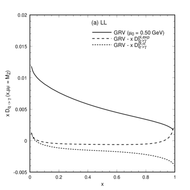
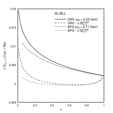
Figure 5: The pointlike quark-to-photon fragmentation function for the up-quark evaluated at $\mu_{F}=M_{Z}$ at (a) LL and (b) BLL. In each case, we show the numerical resummed prediction as well as the difference with the corresponding fixed order expansions given in eqs. (3.14) and (3.16). The hadronic scale is (a) $\mu_{0}=0.50$ GeV for LL GRV and (b) $\mu_{0}=0.55$ GeV for BLL GRV and $\mu_{0}=0.71$ GeV for BLL BFG. In (a) the difference between the LL GRV result and the leading term in the perturbative expansion eq. (3.17) is shown short-dashed.

The expanded expressions for the pointlike part of the quark-to-photon fragmentation function can now be compared directly with the numerical solutions of the LL and BLL resummed expressions for the pointlike fragmentation function for a fixed value of $\mu_{F}$ and over the whole $x$ range. These comparisons are shown in Fig. 5 using the parameterization of the LL and BLL fragmentation functions given by Glück, Reya and Vogt (GRV) in [7] and the BLL parameterization given by Bourhis, Fontannaz and Guillet (BFG) in [3]. In each case, we show the fragmentation function for the up-quark multiplied by the momentum fraction $x$. The other flavours have a similar behaviour. To compare the series expanded fragmentation function with the resummed expression, we also show the differences between the resummed and the expanded solutions given in eqs. (3.14) and (3.16) for the appropriate choices of $\mu_{F}$ and $\mu_{0}$. That is $\mu_{0}=0.50$ GeV for LL GRV, $\mu_{0}=0.55$ GeV for BLL GRV and $\mu_{0}=0.71$ GeV for BLL BFG. In all cases we choose $\mu_{F}=M_{Z}$. As a further comparison, in Fig. 5(a) we also show the difference between the resummed LL fragmentation function and the ${\cal O}(\alpha)$ term of the series expansion,

$$D_{q\to\gamma}^{pl,\alpha}(x,\mu_{F}^{2})=\left(\frac{\alpha e_{q}^{2}}{2\pi}\right)P^{(0)}_{q\to\gamma}\ln\left(\frac{\mu_{F}^{2}}{\mu_{0}^{2}}\right).$$ (3.17)

Inspection of Fig. 5(a) suggests that $D_{q\to\gamma}^{pl,\alpha}$ which is the only term present in the lowest order solution obtained in the fixed order approach is insufficient to correctly reproduce the behaviour of the LL resummed expression. On the other hand, we see that in the region $0.2<x<0.9$ the expanded expression of the fragmentation function is remarkably close to the resummed expression for both LL and BLL pointlike solutions and in the BLL case for the both parameterizations (GRV or BFG). For small $x$, $x<0.2$, there are possible large logarithms of $x$ in addition to contributions from the gluon fragmentation function that are not treated correctly in the expanded result. At large $x$, $x>0.9$, there is also a significant difference between the two approaches. This discrepancy could be a sign that large resummation effects are present. Or it could indicate that the presently available parameterizations for the resummed fragmentation functions are not accurate at large $x$ and particularly for $x>0.95$. In fact, this discrepancy can be traced back to the presence of logarithms of $(1-x)$ that are explicit in the expanded result. These logarithms should also be present in the numerical resummed results. However, the parameterizations are necessarily obtained by inverting only a finite number of moments and it is a well known problem to describe a logarithmic behaviour with a polynomial expansion.

As the resummed fragmentation functions were obtained after the $\ln(\mu_{F}^{2})$ had been resummed, the general agreement with the unsummed and expanded fragmentation functions leads us to question the necessity of such a resummation at LEP energies. Moreover, this agreement in the BLL case has another important consequence. As can be seen from eq. (3.16) the expanded expression for the BLL pointlike quark-to-photon-fragmentation function is also equal to the expression of the next-to-leading perturbative fragmentation function obtained in the fixed order approach as given in eq. (2.12), where the hadronic input is neglected, $D_{q\to\gamma}^{np}(x,\mu_{0})=0$. It is therefore instructive to implement the expanded expression for the quark-to-photon fragmentation function in the evaluation of observable one photon cross sections at LEP energies. Indeed, doing so will enable us to compare the results for these cross sections obtained in different approaches and to isolate easier the differences between them, a task to which we will now turn in Section 4.

4 The cross section in the different approaches compared

We are finally interested in comparing the inclusive and ‘photon’ + 1 jet cross sections evaluated in the two essentially different approaches, at fixed order and following the conventional approach. In Section 2, we have described how the fragmentation function and the one-photon cross section are defined in the fixed order approach, while in Section 3 the derivation of the LL and BLL expressions of the fragmentation function has been discussed. These resummed expressions were determined within the conventional approach, as approximations of the solution of an all-order evolution equation (3.2). By making a Taylor expansion in the strong coupling, analytic expressions for the LL and BLL pointlike solutions were also considered in Section 3.2. Nothing however has been said so far concerning the expressions for the single photon production cross section within this conventional formalism. We shall fulfill this task in this section.

In the following, we shall consider four different classes of expressions for the one-photon production cross section. These classes will be defined depending on whether the resummed (LL or BLL) expressions of the quark-to-photon fragmentation function or the expanded expression of the fragmentation function as given by eq. (3.16) are used in the cross section. Secondly these classes will be determined depending on whether the direct contributions to the cross section are evaluated as a perturbative series in $\alpha_{s}$ up to ${\cal O}(\alpha_{s})$, or whether these direct contributions are evaluated by using a conventional power counting, associating the powers of $\alpha_{s}$ and the powers of $\ln\mu^{2}_{F}$ together. The results obtained for the inclusive and ‘photon’ + 1 jet cross sections following any of these four approaches to evaluate the one-photon production cross section will be compared to the OPAL and ALEPH data in the forthcoming section.

As we will see, in the category of approaches using the expanded expression of the quark-to-photon fragmentation function in the cross section, the specification of the input function $D_{q\to\gamma}^{np}(x,\mu_{0})$ in a given factorization scheme is an important and subtle point which is treated differently by GRV in [7] and by Bourhis, Fontannaz and Guillet BFG in [3]. We shall describe the determination of this input fragmentation function according to either of these two groups in some detail in the second part of this section.

4.1 Approaches using the resummed $D_{q\to\gamma}(x,\mu_{F})$

4.1.1 Direct contributions evaluated at fixed order in $\alpha_{s}$

Let us first concentrate on the expression of the one-photon production cross section in the $\overline{{\rm MS}}$ factorization scheme obtained using the LL or BLL resummed expressions of the quark-to-photon fragmentation function while keeping the direct hard scattering terms building the cross section at fixed order in the strong coupling constant $\alpha_{s}$ up to ${\cal O}(\alpha\alpha_{s})$. In this case the cross section takes the same form as in the fixed order approach described in Section 2, and is described by eq. (2.3) (with $x_{\gamma}$ replaced by $x$) at ${\cal O}(\alpha)$ and by eq. (2.4) at ${\cal O}(\alpha\alpha_{s})$. Rather than the fitted forms (eqs. (2.13) and (2.14)), at ${\cal O}(\alpha)$ the LL fragmentation function should be considered in eq. (2.3), while at ${\cal O}(\alpha\alpha_{s})$ the BLL fragmentation function needs to be taken into account in eq. (2.4). Provided, the solution of the all order evolution equation can be accurately determined, the cross section evaluated following this approach is theoretically preferred as it is the most complete: It includes all direct terms up to order $\alpha\alpha_{s}$ and all fragmentation contributions proportional to $(\alpha_{s}^{n}\ln^{n}\mu_{F}^{2})$ and $(\alpha_{s}^{n}\ln^{n+1}\mu_{F}^{2})$ at all orders.

In order to evaluate either of the single photon production rates according to this prescription, we simply need to replace the fragmentation functions defined at fixed order appearing in these leading and next-to-leading cross sections by the resummed LL or BLL fragmentation functions and leave the remaining terms in the cross sections unchanged. Consequently, by following this approach one is in principle able to test the universality of the LL and BLL fragmentation functions, in particular when these functions are employed to evaluate the ‘photon’ + 1 jet rate, an observable which was not used to determine these functions.

4.1.2 Direct contributions conventionally evaluated

Second, let us consider the expression of the cross section in the $\overline{{\rm MS}}$ scheme arising when one uses the resummed LL or BLL fragmentation functions but when one considers the direct terms of the single photon production cross section evaluated with the conventional power counting. These terms are obtained by keeping only the leading or beyond leading logarithmic terms of the factorization scale $\mu_{F}$ up to a given order in $\alpha_{s}$. As it is commonly done [3, 7], we shall follow this prescription, which defines the conventional approach to obtain the LL and BLL cross sections, and only retain terms proportional to $(\alpha_{s}^{n}\ln^{n+1}\mu_{F}^{2})$ at LL and terms of the form $(\alpha_{s}^{n}\ln^{n+1}\mu_{F}^{2})$ and $(\alpha_{s}^{n}\ln^{n}\mu_{F}^{2})$ in the BLL expression of the cross section.

Remembering furthermore that in this conventional approach, an inverse power of $\alpha_{s}$ is associated with the quark-to-photon fragmentation function as in eq. (3.8), the LL and BLL expressions of the cross section are simply,

$$\frac{1}{\sigma_{0}}\frac{{\rm d}\sigma^{LL}}{{\rm d}x} = \sum_{q=1}^{2N_{f}}\;D_{q\to\gamma}(x,\mu_{F}),$$

$$\frac{1}{\sigma_{0}}\frac{{\rm d}\sigma^{BLL}}{{\rm d}x} = \sum_{q=1}^{2N_{f}}\;\left(D_{q\to\gamma}(x,\mu_{F})\,+\left(\frac{\alpha_{s}}{2\pi}\right)C_{q}^{(0)}\otimes D_{q\to\gamma}(x,\mu_{F})+\left(\frac{\alpha e_{q}^{2}}{2\pi}\right)C^{(0)}_{\gamma}(x,\mu_{F})\right).$$ (4.1)

As already mentioned before, due to the different power of $\alpha_{s}$ associated with the fragmentation function in this approach and in the fixed order approach, the terms present in these two equations and in the corresponding fixed order equations ((2.3) and (2.4)) differ substantially. As explained at length in [6], this conventional procedure of associating an inverse power of $\alpha_{s}$ with the fragmentation function is clearly appropriate when the logarithms of the factorization scale $\mu_{F}$ are the only potentially large logarithms but is theoretically less consistent when different classes of large logarithms can occur as in the ‘photon’ + 1 jet cross section.

4.2 Approaches using the expanded $D_{q\to\gamma}(x,\mu_{F})$

In this subsection, we shall consider the formulations of the cross section obtained using the expanded (up to ${\cal O}(\alpha\alpha_{s})$) expressions of the pointlike and hadronic part of the fragmentation function $D_{q\to\gamma}(x,\mu_{F})$. In particular, we will consider the pointlike part of the fragmentation function given by the expanded expression of the resummed form for the BLL pointlike fragmentation function discussed in Section 3.2 and defined in eq. (3.16). An expanded expression of the hadronic part will be given below. Finally, we shall implement the expanded expression obtained for the sum of pointlike and hadronic parts of the fragmentation function in the NLO and BLL formulations of the cross section given by eqs.(2.4) and (4.1) respectively.

4.2.1 Possible definitions of $D_{q\to\gamma}^{np}(x,\mu_{0})$

In order to obtain a definite prediction for the cross section using either the GRV or BFG models of the quark-to-photon fragmentation function, we need to know how the hadronic part of the fragmentation function behaves and in particular we need to know how the input function $D_{q\to\gamma}^{np}(x,\mu_{0})$ is defined. Since within this context we have an expanded (up to ${\cal O}(\alpha\alpha_{s})$) form for the pointlike part of the fragmentation function, we here choose to consider also an expanded expression (up to ${\cal O}(\alpha\alpha_{s})$) for the hadronic part of this function, given by,

$$D_{q\to\gamma}^{had,(exp.)}(x,\mu_{F})=D_{q\to\gamma}^{np}(x,\mu_{0})+\left(\frac{\alpha_{s}}{2\pi}\right)\ln\left(\frac{\mu^{2}_{F}}{\mu_{0}^{2}}\right)P^{(0)}_{q\to q}\otimes D_{q\to\gamma}^{np}(x,\mu_{0})+{\cal O}(\alpha\alpha_{s}^{2}).$$ (4.2)

This expression is obtained by expanding eq. (LABEL:eq:dhadbll) and takes exactly the same form as the non-perturbative part of the fragmentation function defined in the fixed order approach described in Section 2. Recall that in the fixed order approach, the input fragmentation function $D_{q\to\gamma}^{np}(x,\mu_{0})$ present as a boundary condition in eq. (4.2) was determined at each order by comparing the fixed order ‘photon’ +1 jet cross section with the ALEPH data, with leading order and next-to-leading order expressions given in equations (2.13) and (2.14) respectively. Note also that the fitted input fragmentation function determined within this fixed order context is clearly non-negligible at any order in $\alpha_{s}$.

In the approaches of GRV or BFG , the treatment of the input fragmentation function $D_{q\to\gamma}^{np}(x,\mu_{0})$ is quite different. At LL both GRV and BFG agree that $D_{q\to\gamma}^{np}(x,\mu_{0})$ is negligible and can be described by a vector meson dominance model (VMD) as explained in [3] and [7] respectively. However at BLL and in the $\overline{{\rm MS}}$ scheme, the input fragmentation function cannot be negligible due to the presence of the direct term $C_{\gamma}^{(0)}$ (see eqs. (2.3), (2.4) or (4.1)) and cannot be described by a VMD input alone. Indeed, $C_{\gamma}^{(0)}$ diverges as $x\to 1$ and would drive the cross section to unacceptable negative values if a VMD input alone is considered for the input fragmentation function. Note that the requirement that the cross section is positive led the authors in [5, 6] to consider a term proportional to $P^{(0)}_{q\to\gamma}\ln(1-x)^{2}$ in the expression of $D_{q\to\gamma}^{np}(x,\mu_{0})$. To summarize the discussion, in any resummed or fixed order approach, as soon as the direct term $C_{\gamma}^{(0)}$ enters the cross section, as it does in the $\overline{{\rm MS}}$ factorization scheme, the input fragmentation function $D_{q\to\gamma}^{np}(x,\mu_{0})$ must compensate the large $x$ behaviour of $C_{\gamma}^{(0)}$.

So far all the formulae given for the cross section were given in the $\overline{{\rm MS}}$ factorization scheme. It is well known however, that the direct and fragmentation contributions are not unequivocally defined. For instance in a different factorization scheme, $S$ a part of $C_{\gamma}^{(0)}$ (direct term) $\Delta C_{\gamma}^{(0)}\mid_{S}$ can be absorbed in the fragmentation function yielding new functions $D_{q\to\gamma}(x,\mu_{F})\mid_{S}$ and $C_{\gamma}^{(0)}\mid_{S}(x,\mu_{F})$, so that,

$$D_{q\to\gamma}(x,\mu_{F})\mid_{S}=D_{q\to\gamma}(x,\mu_{F})\mid_{\overline{{\rm MS}}}+\left(\frac{\alpha e_{q}^{2}}{2\pi}\right)\Delta C_{\gamma}^{(0)}\mid_{S}(x)$$ (4.3)

and,

$$C_{\gamma}^{(0)}\mid_{S}(x,\mu_{F})=C_{\gamma}^{(0)}\mid_{\overline{{\rm MS}}}(x,\mu_{F})-\Delta C_{\gamma}^{(0)}\mid_{S}(x).$$ (4.4)

In fact only the combination of both direct and fragmentation contributions present in the physical cross section is factorization scheme invariant. The approaches adopted by GRV or BFG use this factorization scheme ambiguity to determine $D_{q\to\gamma}^{np}(x,\mu_{0})$, albeit in a slightly different way.

The GRV group choose to work within a factorization scheme (called $DIS_{\gamma}$) in which the fragmentation input $D_{q\to\gamma}^{np}(x,\mu_{0})$ at both LL and BLL is simply given by a VMD contribution and is therefore negligible. Essentially, within this new scheme the troublesome part of the direct contribution $C_{\gamma}^{(0)}$ appearing in eq. (4.1) is removed by absorbing it into the definition of the quark-to-photon fragmentation function $D_{q\to\gamma}(x,\mu_{F})$. More precisely, in this scheme we have,

$$\Delta C_{\gamma}^{(0)}\mid_{DIS_{\gamma}}(x)=P^{(0)}_{q\to\gamma}(x)\ln\left((1-x)x^{2}\right)-2\left(\frac{1-x}{x}\right),$$ (4.5)

and,

$$D_{q\to\gamma}^{np}(x,\mu_{0})\mid_{DIS_{\gamma}}=D_{q\to\gamma}^{np}(x,\mu_{0})\mid_{\overline{{\rm MS}}}+\;\left(\frac{\alpha e_{q}^{2}}{2\pi}\right)\Delta C_{\gamma}^{(0)}\mid_{DIS_{\gamma}}(x)\sim D_{q\to\gamma}^{VMD}.$$ (4.6)

This transformation holds for any quark flavour. Within this scheme, the direct term $C_{\gamma}^{(0)}\mid_{DIS_{\gamma}}$ is regular as $x\to 1$. The evolution equation of the quark-to-photon fragmentation function in the $S$-scheme is modified as well,

$$P^{(1)}_{q\to\gamma}\mid_{S}=P^{(1)}_{q\to\gamma}\mid_{\overline{{\rm MS}}}\;-\,\left(\frac{\alpha e_{q}^{2}}{2\pi}\right)\Delta C_{\gamma}^{(0)}\mid_{S}\otimes P^{(0)}_{q\to q}.$$ (4.7)

Invoking a perturbative stability argument, this group considers the evolution equation in the $DIS_{\gamma}$-scheme, solves this equation in that scheme and then since the $\overline{{\rm MS}}$-scheme is traditionally preferred in the evaluation of cross sections at higher orders, transforms back their results to the $\overline{{\rm MS}}$-scheme according to eq. (4.3). For illustration, the GRV up-quark fragmentation function at $\mu_{F}=M_{Z}$ and in both the $DIS_{\gamma}$ and $\overline{{\rm MS}}$ factorization schemes is shown in Fig. 6.

Note that, to obtain the results in the $DIS_{\gamma}$ scheme, we have added a term proportional to $\Delta C_{\gamma}^{(0)}\mid_{DIS_{\gamma}}(x)$ to the $\overline{{\rm MS}}$ fragmentation function provided numerically by GRV. We see that the difference between the full and pointlike fragmentation functions due only to the VMD input is small in either scheme, and particularly at large $x$. Furthermore, we see that although the fragmentation function in one scheme may be well behaved as $x\to 1$, in a different scheme, it will diverge as $\ln(1-x)$. Surprisingly, it appears well behaved in the $\overline{{\rm MS}}$-scheme rather than the specially constructed $DIS_{\gamma}$ scheme. As discussed earlier, this is due to an inaccuracy in the numerical resummed results produced by inverting only a finite number of moments. If the large $x$ region is treated correctly, the $DIS_{\gamma}$ fragmentation function should be well behaved while the $\overline{{\rm MS}}$ fragmentation function will exhibit a logarithmic enhancement.

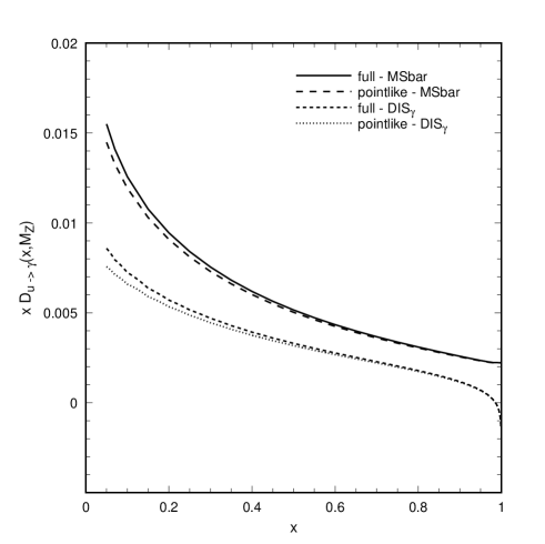
Figure 6: The GRV up quark-to-photon fragmentation function $xD_{u\to\gamma}(x,\mu_{F})$ evaluated $\mu_{F}=M_{Z}$. The full (pointlike) fragmentation function is shown as a solid (dashed) line in the $\overline{{\rm MS}}$-scheme and as a short-dashed (dotted) line in the $DIS_{\gamma}$-scheme (see text).

In order to be able to implement an expanded form for the complete quark-to-photon fragmentation function in the BLL and NLO $(\overline{{\rm MS}})$ expressions of the cross section given by eqs. (2.4), (4.1) we need to know such a form in that scheme. The sum of the expanded expressions for the pointlike and hadronic parts of the fragmentation function given in eqs. (3.16) and (4.2) in the $\overline{{\rm MS}}$-scheme reads,

$$D_{q\to\gamma}^{(exp.)}\mid_{\overline{{\rm MS}}}(x,\mu_{F})=D_{q\to\gamma}^{pl,(exp.)}\mid_{\overline{{\rm MS}}}(x,\mu_{F})+D_{q\to\gamma}^{had,(exp.)}\mid_{\overline{{\rm MS}}}(x,\mu_{F}).$$ (4.8)

Rewriting the hadronic input in the $DIS_{\gamma}$ scheme yields,

$$D_{q\to\gamma}^{(exp.)}\mid_{\overline{{\rm MS}}}(x,\mu_{F}) = D_{q\to\gamma}^{pl,(exp.)}\mid_{\overline{{\rm MS}}}(x,\mu_{F})$$ (4.9)

$$- \left(\frac{\alpha e_{q}^{2}}{2\pi}\right)\Delta C_{\gamma}^{(0)}\mid_{DIS_{\gamma}}(x)$$

$$- \left(\frac{\alpha e_{q}^{2}}{2\pi}\right)\left(\frac{\alpha_{s}}{2\pi}\right)\ln\left(\frac{\mu^{2}_{F}}{\mu_{0}^{2}}\right)P^{(0)}_{q\to q}\otimes\Delta C_{\gamma}^{(0)}\mid_{DIS_{\gamma}}(x)$$

$$+ D_{q\to\gamma}^{np}\mid_{DIS_{\gamma}}(x,\mu_{0})$$

$$+ \left(\frac{\alpha_{s}}{2\pi}\right)\ln\left(\frac{\mu^{2}_{F}}{\mu_{0}^{2}}\right)P^{(0)}_{q\to q}\otimes D_{q\to\gamma}^{np}\mid_{DIS_{\gamma}}(x,\mu_{0}).$$

The last two lines of this equation are proportional to the VMD input, $D_{q\to\gamma}^{np}\mid_{DIS_{\gamma}}(x,\mu_{0})$, which is negligible [7], and can be neglected. Note that, an equivalent way to obtain this expression, with the model-dependent input $D_{q\to\gamma}^{np}\mid_{DIS_{\gamma}}(x,\mu_{0})$ neglected, is to consider $D_{q\to\gamma}^{np}(x,\mu_{0})\mid_{\overline{{\rm MS}}}$ to be given simply by $-\Delta C_{\gamma}^{(0)}\mid_{DIS_{\gamma}}$.

4.2.2 Direct contributions evaluated conventionally

The expression for the BLL single-photon production cross section in the $\overline{{\rm MS}}$-scheme obtained using a conventional power counting of the direct terms and using the expanded expression of the fragmentation function given in eq. (4.9) (with $D_{q\to\gamma}^{np}\mid_{DIS_{\gamma}}(x,\mu_{0})=0$) then reads,

$$\frac{1}{\sigma_{0}}\frac{{\rm d}\sigma^{BLL(exp.)}}{{\rm d}x} = \sum_{q=1}^{2N_{f}}\left(-\left(\frac{\alpha e_{q}^{2}}{2\pi}\right)\Delta C_{\gamma}^{(0)}\mid_{DIS_{\gamma}}-\left(\frac{\alpha e_{q}^{2}}{2\pi}\right)\left(\frac{\alpha_{s}}{2\pi}\right)\ln\left(\frac{\mu^{2}_{F}}{\mu_{0}^{2}}\right)P^{(0)}_{q\to q}\otimes\Delta C_{\gamma}^{(0)}\mid_{DIS_{\gamma}}(x)\right.$$ (4.10)

$$+\left(\frac{\alpha e_{q}^{2}}{2\pi}\right)\ln\left(\frac{\mu^{2}_{F}}{\mu_{0}^{2}}\right)P^{(0)}_{q\to\gamma}(x)+\left(\frac{\alpha e_{q}^{2}}{2\pi}\right)\left(\frac{\alpha e_{q}^{2}}{2\pi}\right)\ln\left(\frac{\mu^{2}_{F}}{\mu_{0}^{2}}\right)P^{(1)}_{q\to\gamma}(x)$$

$$+\frac{1}{2}\left(\frac{\alpha e_{q}^{2}}{2\pi}\right)\left(\frac{\alpha_{s}}{2\pi}\right)\ln^{2}\left(\frac{\mu^{2}_{F}}{\mu_{0}^{2}}\right)P^{(0)}_{q\to q}\otimes P^{(0)}_{q\to\gamma}(x)$$

$$\left.+\left(\frac{\alpha e_{q}^{2}}{2\pi}\right)\left(\frac{\alpha_{s}}{2\pi}\right)\ln\left(\frac{\mu^{2}_{F}}{\mu_{0}^{2}}\right)C_{q}^{(0)}\otimes P^{(0)}_{q\to\gamma}(x)+\left(\frac{\alpha e_{q}^{2}}{2\pi}\right)C^{(0)}_{\gamma}(x,\mu_{F})\right).$$

where we have only retained terms proportional to $\alpha_{s}^{0}$, $(\alpha_{s}^{0}\ln\mu_{F}^{2})$, $(\alpha_{s}^{1}\ln\mu_{F}^{2})$ and $(\alpha_{s}^{1}\ln^{2}\mu_{F}^{2})$.

4.2.3 Direct contributions evaluated at fixed order in $\alpha_{s}$

The corresponding next-to-leading order expression for the cross section can however not be directly obtained by implementing the expanded quark-to-photon fragmentation function of eq. (4.9) in the next-to-leading order $\overline{{MS}}$ cross section given in eq. (2.4). We need to consider a further modification to the direct term present in eq. (2.4) which is generated by the transformation of the non-perturbative input from the $\overline{{MS}}$-scheme to the $DIS_{\gamma}$-scheme, eq. (4.6). With this change, the term proportional to $C_{q}^{(0)}\otimes D_{q\to\gamma}(x,\mu_{F})$ in eq. (4.1) becomes,

$$+\left(\frac{\alpha e_{q}^{2}}{2\pi}\right)\left(\frac{\alpha_{s}}{2\pi}\right)C_{q}^{(0)}\otimes\left[P^{(0)}_{q\to\gamma}(x)\ln\left(\frac{\mu^{2}_{F}}{\mu_{0}^{2}}\right)+D_{q\to\gamma}^{np}\mid_{DIS_{\gamma}}(x,\mu_{0})-\Delta C_{\gamma}^{(0)}\mid_{DIS_{\gamma}}\right].$$

Here, the term proportional to $C_{q}^{(0)}\otimes\Delta C_{\gamma}^{(0)}$ is genuinely of ${\cal O}(\alpha_{s})$ and unlike the term proportional to $P^{(0)}_{q\to\gamma}$ could be ignored in the conventional BLL approach discussed above. However, for a consistent treatment at fixed NLO, it must be retained, so that, in the $\overline{{MS}}$-scheme,

$$\frac{1}{\sigma_{0}}\frac{{\rm d}\sigma^{NLO(exp.)}}{{\rm d}x}=\frac{1}{\sigma_{0}}\frac{{\rm d}\sigma^{BLL(exp.)}}{{\rm d}x}+\left(\frac{\alpha e_{q}^{2}}{2\pi}\right)\left(\frac{\alpha_{s}}{2\pi}\right)C_{\gamma}^{(1)}-\left(\frac{\alpha e_{q}^{2}}{2\pi}\right)\left(\frac{\alpha_{s}}{2\pi}\right)C_{q}\otimes\Delta C_{\gamma}^{(0)}\mid_{DIS_{\gamma}}.$$ (4.11)

Here, we clearly see which terms differ between the BLL and NLO cross sections when using an expanded expression for the fragmentation function. Another way to understand the origin of this additional term is gained by considering the expressions of the next-to-leading order cross section ${\rm d}{\sigma}^{NLO}$ in both $\overline{{\rm MS}}$ and $DIS_{\gamma}$-schemes. The requirement that these two quantities are equal, dictates that,

$$\left(\frac{\alpha e_{q}^{2}}{2\pi}\right)\left(\frac{\alpha_{s}}{2\pi}\right)C_{\gamma}^{(1)}+\left(\frac{\alpha_{s}}{2\pi}\right)C_{q}\otimes D_{q\to\gamma}(x,\mu_{F})$$

has to be invariant under the scheme transformation. Equivalently we have,

$$C_{\gamma}^{(1)}\mid_{DIS_{\gamma}}=C_{\gamma}^{(1)}\mid_{\overline{{\rm MS}}}-C_{q}\otimes\Delta C_{\gamma}^{(0)}\mid_{DIS_{\gamma}}.$$ (4.12)

Let us now turn to the approach followed by BFG to determine $D_{q\to\gamma}(x,\mu_{F})$. Unlike the GRV group they consider the evolution of the quark-to-photon fragmentation function directly in the $\overline{{\rm MS}}$-scheme with a non-perturbative input given by,

$$D_{q\to\gamma}^{np}\mid_{\overline{{\rm MS}}}(x,\mu_{0})\equiv D_{q\to\gamma}^{VMD}(x,\mu_{0})-C_{\gamma}^{(col)}(x),$$ (4.13)

where $D_{q\to\gamma}^{VMD}$ is fixed by a vector dominance model and is negligible. Effectively, the input is $-C_{\gamma}^{(col)}$, the collinear part of the direct term $C_{\gamma}^{(0)}$ which is defined in eq. (2.16) and again diverges logarithmically as $x\to 1$.

As mentioned before, the GRV group uses the same input and the same evolution equation for each quark flavour as we do in the fixed order approach. Unlike in our fixed order approach, where all 5 flavours are treated massless, the GRV group considers the masses of charm and bottom quarks ($m_{c}=1.5$ GeV and $m_{b}=4.5~{}$GeV) and let the evolution equations of the heavy flavour fragmentation functions start at the appropriate mass thresholds [7]. In other words, for the charm-to-photon and the bottom-to-photon fragmentation function, they select $\mu_{0}=m_{c},m_{b}$ respectively. The BFG group also considers the charm and bottom quarks to be massive. However, in their approach, the input distribution given in eq. (4.13) is valid only for light quarks and the heavy quark input is treated slightly differently as explained in [3]. For most applications though, (such as single photon production at LEP energies) we are far from the quark mass thresholds and the massless evolution of the charm and bottom fragmentation functions is a good approximation. For this reason we will not go into the details of the treatment of heavy quarks in the BFG approach and merely refer the reader to the original work [3].

For reference, we show the full and pointlike up-quark fragmentation functions in Fig. 7 at $\mu_{F}=M_{Z}$. Here, the difference between the curves is not due to $D_{q\to\gamma}^{VMD}$ alone, but depends on the combination, $D_{q\to\gamma}^{VMD}(x,\mu_{0})-C_{\gamma}^{(col)}(x)$. This should engender a significant difference at large $x$, but, because of the difficulty of obtaining accurate parameterizations at large $x$ numerically, this has been obscured.

Figure 7: The BFG up quark-to-photon fragmentation function $xD_{u\to\gamma}(x,\mu_{F})$ evaluated at $\mu_{F}=M_{Z}$. The full (pointlike) fragmentation function is shown as a solid (dashed) line in the $\overline{{\rm MS}}$-scheme.

The analogues of the BLL and NLO expanded expressions of the single photon production cross section following the BFG approach (at least for the light quark) are obtained by replacing $\Delta C_{\gamma}^{(0)}\mid_{DIS_{\gamma}}$ by $C_{\gamma}^{(col)}$ in eqs. (4.10) and (4.11). A similar transformation accompanied by replacing $D_{q\to\gamma}^{np}(x,\mu_{0})\mid_{DIS_{\gamma}}$ by $D_{q\to\gamma}^{VMD}(x,\mu_{0})$ in eq. (4.9) yields an expression for the $\overline{{\rm MS}}$ quark-to-photon fragmentation function in the BFG approach. Finally, note that the only difference between the expression of the NLO single photon production cross section obtained following the fixed order approach with the BFG non-perturbative input given in eq. (4.13) and that obtained in the fixed order approach as described in Section 2 is the different non-perturbative input which in our approach is determined by the ALEPH data, see eq. (2.14).

4.3 Summary

The different strategies for evaluating the single photon cross section described in this section can be summarized as follows;

• Resummed fragmentation function obtained numerically together with explicit power counting of the coupling constants, as described in sec. 4.1.1 and at NLO by eq. (2.4)).

• Resummed fragmentation function with conventional power counting, i.e. associating an inverse power of $\alpha_{s}$ with $D_{q\to\gamma}$. See sec. 4.1.2 and eq. (4.1) for the BLL result.

• Fragmentation function expanded as a series in $\alpha_{s}$ (given in eq. (4.9) and with the non-perturbative input $D_{q\to\gamma}^{np}\mid_{DIS_{\gamma}}(x,\mu_{0})$ neglected) together with conventional power counting, i.e. associating an inverse power of $\alpha_{s}$ with each power of $\ln\mu_{F}^{2}$. See sec. 4.2.2 and eq. (4.10).

• Expanded fragmentation function together with explicit power counting of the coupling constants, as described in sec. 4.2.3 and eq. (4.11).

Provided the resummed solution of the all order evolution equation can be accurately determined, the approach using this solution and the direct terms evaluated at fixed order (approach I) represents the theoretically preferred approach. The approach evaluating the direct terms at fixed order and using an expanded and thereby approximate expression of the fragmentation function has however important advantages. It enables an analytic determination of the fragmentation function and yields factorization scale independent results for the photon production cross section evaluated at a given order in $\alpha_{s}$. Furthermore, the implementation of the non-perturbative quark-to-photon fragmentation function which was fitted to the ALEPH ‘photon’ + 1 jet in the fixed order expressions of the ‘isolated’ and inclusive rate yielded perturbative stable predictions [6] which agreed well with the ALEPH and OPAL data.

In the next section we shall see how the theoretical predictions obtained following any of these approaches and using the GRV or BFG schemes compare with the OPAL and ALEPH data. For definiteness, in approaches I and II we will use either the parameterization of the pointlike fragmentation function of the GRV group or the sum of pointlike and hadronic parts (set I) of the BFG group. In approaches III and IV, we will consider eq. (4.9) with the VMD input $D_{q\to\gamma}^{np}\mid_{DIS_{\gamma}}(x,\mu_{0})$ set to zero to describe the evolution equations for all active flavours in the GRV case, and the same equation with $\Delta C_{\gamma}^{(0)}\mid_{DIS_{\gamma}}$ replaced by $C_{\gamma}^{(col)}$ in the BFG case. As a result, in these approaches and in either of the two schemes all quark flavours satisfy a massless evolution equation. Finally, the light flavours start their evolution at $\mu_{0}=0.55$ GeV and at $\mu_{0}=0.71$ GeV respectively in the GRV or in the BFG schemes, while the heavy $c$ and $b$ quark fragmentation functions start to evolve at $\mu_{0}=m_{c}$ and $\mu_{0}=m_{b}$ respectively.

5 Results

In the previous sections we have completed a detailed comparison of the two fundamentally different approaches (fixed order and conventional) for computing photon cross sections. We have described how both the cross sections and fragmentation functions are defined in these two formalisms and in Section 4 we have given expressions for the cross section obtained using an expanded expression for the quark-to-photon fragmentation function $D_{q\to\gamma}(x,\mu_{F})$. We have now collected all necessary ingredients to be able to evaluate the single photon production cross section in any of the four approaches summarized in Section 4.3 and could perform this task while defining the non-perturbative input according to either of the GRV or BFG groups. We shall apply these calculations to compute both the inclusive cross section and the ‘photon’ + 1 jet rate and make comparisons with the OPAL and ALEPH data in the second part of this section.

Before turning to the cross sections, we first compare the analytic expanded expression of the quark-to-photon fragmentation function given by eq. (4.9) with the numerically resummed BLL results for both GRV and BFG prescriptions. This is shown in Fig. 8 for the up-quark. Note that in addition to fixing the non-VMD input, $\Delta C_{\gamma}^{(0)}\mid_{S}$ differently in the two schemes, the hadronic scale is also different, $\mu_{0}=0.55$ GeV for BLL GRV and $\mu_{0}=0.71$ GeV for BLL BFG. There are two ranges of interest, $0.2<x<0.95$ which is relevant for the inclusive photon data from OPAL and $0.7<x<1$ appropriate for the ALEPH ‘photon’ + 1 jet data.

We see that, except in the very high $x$ region, the various fragmentation functions generally agree well with each other in shape and magnitude. As discussed earlier, at large $x$, there are significant disagreements which are mainly due to deficiencies in the numerical parameterizations. We therefore expect, that predictions for the inclusive photon cross sections (which run over a wide range of $x$) will be largely in agreement, while significant differences may be apparent in the ‘photon’ + 1 jet estimates which focus on the large $x$ region.

We also see that the expanded fragmentation functions defined according to the BFG and GRV prescriptions are quite different. This is in part due to the different choice of hadronic scale, but mainly due to the fact that the non-VMD BFG input is more negative than that for GRV. As can be seen from eq. (4.9) and the definitions of $\Delta C_{\gamma}^{(0)}\mid_{DIS_{\gamma}}$ and $C_{\gamma}^{(col)}$, then for the same hadronic scale,

$$D_{q\to\gamma}^{(exp.)GRV}\mid_{\overline{{\rm MS}}}(x,\mu_{F})-D_{q\to\gamma}^{(exp.)BFG}\mid_{\overline{{\rm MS}}}(x,\mu_{F})>0.$$ (5.1)

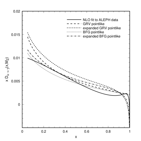
Figure 8: The quark-to-photon fragmentation function $xD_{u\to\gamma}(x,\mu_{F})$ evaluated at $\mu_{F}=M_{Z}$ in the $(\overline{{\rm MS}})$-scheme. The NLO fit from the ALEPH ‘photon’ + 1 jet data is shown as solid line. The pointlike GRV (BFG) parameterization is shown dashed (dotted) while the expanded result of eq. (4.9) is shown short-dashed (dot-dashed).

5.1 The inclusive cross sections

In this subsection we collect the results obtained evaluating the inclusive one-photon production cross sections following any of the four approaches described in Section 4.

So far, we have ignored the gluon-to-photon fragmentation function throughout. To illustrate the tiny role the gluon-to-photon fragmentation plays in a physical cross section, Fig. 9 shows the BLL prediction for the inclusive rate for the pointlike GRV parameterization both with and without the gluon-to-photon fragmentation contribution. To make the small difference manifest, we have multiplied the gluon-to-photon fragmentation contribution by a factor of 100. We see that at large $E_{\gamma}$, even when multiplied by a factor of 100, the gluon fragmentation contribution is entirely negligible. At lower energies, the gluon fragmentation reduces the cross section by at most 5% at $E_{\gamma}\sim 10$ GeV. Similar results are also obtained at LL. In the following we shall therefore ignore the gluon-to-photon fragmentation contribution to the photon production cross section.

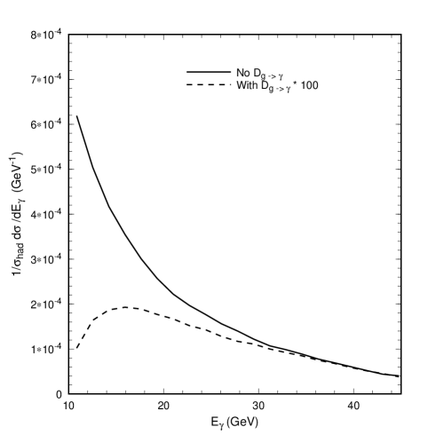
Figure 9: The BLL prediction for the inclusive rate evaluated at $\mu_{F}=M_{Z}$ using the pointlike GRV parameterization with the gluon-to-photon fragmentation function ignored (solid) and multiplied by 100 (dashed). The experimental data is taken from [2].

5.1.1 Perturbative stability and $\mu_{F}$-dependence

The results obtained using the GRV parameterization together with conventional power counting at LL and BLL (i.e. approach II) are shown in Fig. 10. The upper/lower curves correspond to varying the factorization scale in the range $2M_{Z}/0.5M_{Z}$. We see that the LL and BLL predictions are similar and thus appear to be perturbatively stable. Furthermore, the factorization scale dependence is significantly reduced in going from LL to BLL.

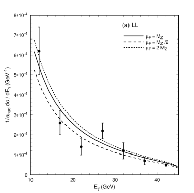
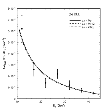
Figure 10: The (a) LL and (b) BLL predictions for the inclusive photon rate using the pointlike GRV parameterization and conventional power counting. The solid lines show the prediction for $\mu_{F}=M_{Z}$, while the short-dashed (long-dashed) lines show the expected rate for $\mu_{F}=2M_{Z}~{}(0.5M_{Z}$). The experimental data is taken from [2].

Let us see what happens when the inclusive rate is evaluated in approach I, i.e. using the resummed LL and BLL fragmentation function but with the direct contributions evaluated at fixed order. This is shown in Fig. 11 at LO and NLO for the same three choices of the factorization scale as in Fig. 10. In this case, it appears that we can draw the same conclusion regarding the $\mu_{F}$ dependence, it is reduced in going from LO to NLO. However, the LO and NLO results appear to be significantly different over the whole range of $E_{\gamma}$. This difference is caused by the presence of the direct term $C_{\gamma}^{(0)}$ in the LO and NLO expressions of the cross section (see eq. (2.3) and (2.4)). The failure to describe the inclusive data with the LL resummed fragmentation function and with the direct contributions evaluated at lowest order in the expression of the cross section indicate that the direct and fragmentation contributions are not properly matched to each other when the cross section is evaluated in this way.

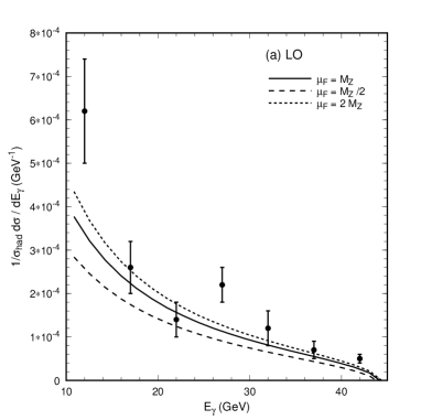
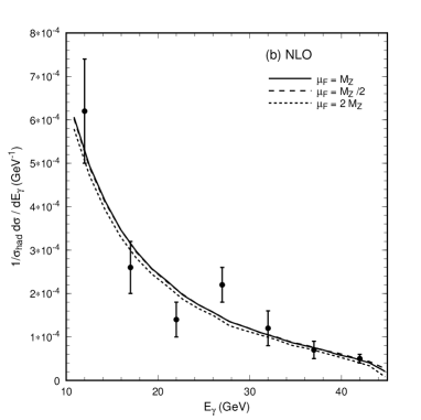
Figure 11: The (a) LO and (b) NLO predictions for the inclusive photon rate using the pointlike GRV parameterization and explicit power counting. The solid lines show the prediction for $\mu_{F}=M_{Z}$, while the short-dashed (long-dashed) lines show the expected rate for $\mu_{F}=2M_{Z}~{}(0.5M_{Z}$). The experimental data is taken from [2].

5.1.2 Comparison of results

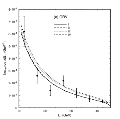
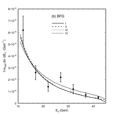
Figure 12: The inclusive photon spectrum estimated from the four approaches discussed in sec. 4 using (a) the GRV and (b) the BFG parameterizations. The experimental data is taken from [2].

Fig. 12 shows the (NLO or BLL) inclusive cross section obtained using each of the four approaches described in Section 4 for $\mu_{F}=M_{Z}$. We show the predictions using both the GRV and BFG schemes while considering in each case the definitions of the fragmentation function given in Section 4. The various approaches give predictions which have a similar shape and lie in a common band which is well contained within the experimental error bars over the whole $x$ range of the OPAL data. The agreement between the predictions is largely due to the similarity between the fragmentation functions as shown in Fig. 8 but also because the leading direct term $C_{\gamma}^{(0)}$ is included in each approach. We note that the cross section obtained using the expanded expression for the fragmentation function (III and IV) lies by an almost constant amount above the prediction obtained using the resummed fragmentation functions (I and II) over the whole $x$ range of interest. However, given the size of the experimental errors, all four predictions appear to describe the OPAL data equally well.

5.2 The ‘photon’ + 1 jet rates

Let us now present the results obtained for the ‘photon’ + 1 jet rate. In the following, we focus on one particular value of the jet clustering parameter $y_{\rm cut}$, $y_{\rm cut}=0.1$. We note that in the range of interest for the ALEPH data, $0.7<z<1$ the difference between the results obtained using the pointlike quark-to-photon fragmentation functions alone or the full fragmentation function (i.e. sum of pointlike and and hadronic parts) is small. Furthermore, the gluon-to-photon fragmentation plays an entirely negligible role.

5.2.1 Perturbative stability and $\mu_{F}$ dependence

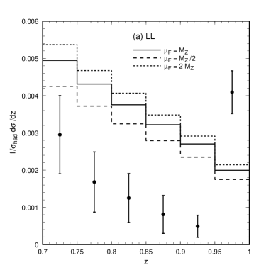
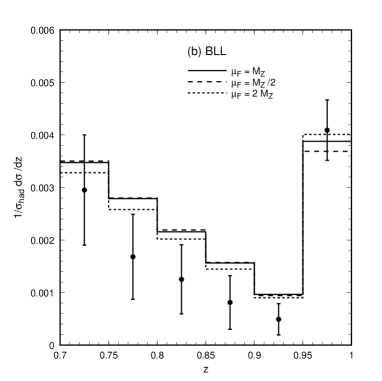
Figure 13: The (a) LL and (b) BLL predictions for the ‘photon’ + 1 jet rate using the pointlike GRV parameterization and conventional power counting. The solid lines show the prediction for $\mu_{F}=M_{Z}$, while the short-dashed (long-dashed) lines show the expected rate for $\mu_{F}=2M_{Z}~{}(0.5M_{Z}$). The experimental data is taken from [1].

Predictions for the ‘photon’ + 1 jet rate using the pointlike GRV parameterization together with conventional power counting at LL and BLL (i.e. approach II) are shown in Fig. 13. We vary the factorization scale over a factor of 2 of the central scale $\mu_{F}=M_{Z}$, and, as before, the factorization scale dependence is significantly reduced in going from LL to BLL. However, the difference between the LL and BLL results is sizeable and the shape completely different. In particular, the BLL prediction does match the shape of the data quite well.

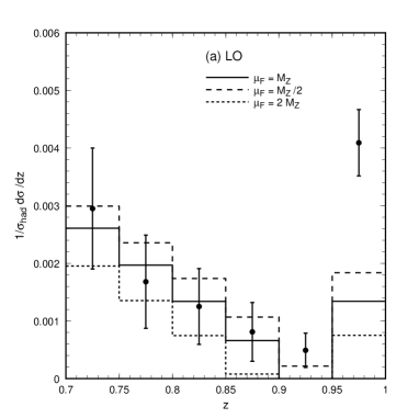
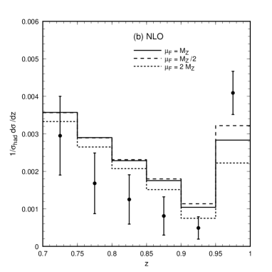
Figure 14: The (a) LO and (b) NLO predictions for the ‘photon’ + 1 jet rate using the pointlike GRV parameterization and conventional power counting. The solid lines show the prediction for $\mu_{F}=M_{Z}$, while the short-dashed (long-dashed) lines show the expected rate for $\mu_{F}=2M_{Z}~{}(0.5M_{Z}$). The experimental data is taken from [1].

Let us now analyze what happens if one considers the resummed expression for the GRV fragmentation function in an expression of the cross section where the direct terms are evaluated at fixed order in $\alpha_{s}$ (i.e. approach I). Fig. 14 shows the LO and NLO ‘photon’ + 1 jet predictions for the same three values of the factorization scale $\mu_{F}$. As can be seen by comparing the leading and next-to-leading order results, the factorization scale dependence is significantly reduced. We also see that the shapes of the curves displayed at leading and next-to-leading order are not dramatically changed. This could be viewed as an indication that the results obtained in this approach are perturbatively stable. For $\mu_{F}=M_{Z}$ we find that, the lowest order prediction appears to be slightly below the data while the next-to-leading order result lies above the data.

5.2.2 Comparison of results

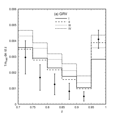
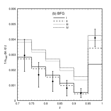
Figure 15: The ‘photon’ + 1 jet rate estimated from the four approaches discussed in sec. 4 using (a) the GRV (b) the BFG inputs. The experimental data is taken from [1].

Fig. 15 shows the (NLO or BLL) ‘photon’ + 1 jet rates obtained using each of the four approaches described in Section 4 for $\mu_{F}=M_{Z}$, with the fragmentation functions used in each approach as defined in Section 4. Ignoring the large $z$ region where we have reason to doubt the accuracy of the parameterizations in methods I and II, we see that the BFG predictions lie systematically below that obtained using the GRV parameterization and go through the experimental data points. As discussed earlier, this difference is due to both the choice of hadronic scale and the non-VMD input. The BFG input is smaller and the ‘photon’ + 1 jet data clearly selects this choice. Notice however, that the BFG parameterization for the fragmentation function unlike that of the GRV group was proposed well after the ALEPH data were released. As in the inclusive photon rate, predictions involving the expanded fragmentation function (approaches III and IV) always lie above the corresponding approach using the resummed fragmentation function (I and II). Again, the data clearly prefers the resummed fragmentation function. However, the shape of the predictions obtained with an expanded fragmentation function indicates that adding a negative constant to them would describe the data very well.

6 Conclusions

In this paper we have made a detailed study of photon production in hadronic events in electron-positron annihilation at LEP energies. First, we have used the fixed order approach of [5, 6, 10] to estimate the inclusive photon spectrum and to compare it with the recent OPAL data [2]. Here, the fragmentation function is determined at large $x$ ($x>0.7$) by the ALEPH ‘photon’ + 1 jet data [1] and is an exact solution of the evolution equation without resummation of logarithms of the factorization scale. As such, the prediction is scale independent and, surprisingly, agrees well with the OPAL data which corresponds to $x$ values as small as 0.2. This is a powerful indication that the fragmentation function fitted to the ALEPH data is process independent and can be used to predict photon cross sections in other processes.

Alternative methods to compute inclusive photon cross sections rely on numerically solving the evolution equations with some non-perturbative input. This input has two pieces, a small vector meson dominance contribution together with a perturbative counterterm. Different parameterizations deal with this ambiguity in different ways. We have examined the choices made by the BFG and GRV groups and used them to compute both the inclusive photon and ‘photon’ + 1 jet rates. To check the general behaviour of the fragmentation function, we have made an analytic series expansion in the strong coupling. As a result, we find that the large $x$ behaviour of the fragmentation functions is not well reproduced by the parameterizations, the main problem being to describe a logarithmic behaviour with a polynomial.

An additional subtlety is that although the fragmentation function appears to be ${\cal O}(\alpha)$, inspection of the evolution equation suggests a logarithmic growth with $\mu_{F}$, and in many analyzes, it is ascribed a nominal power of $\alpha/\alpha_{s}$. Constructing the cross section at some particular order depends on this assignment and different terms will contribute. This was discussed at length in Section 4. In addition, the gluon-to-photon fragmentation function is naively of ${\cal O}(\alpha\alpha_{s})$ and is expected to be much smaller than the quark contribution. This is indeed the case for physical cross sections in electron-positron annihilation where gluon production is suppressed, and we ignore the gluon fragmentation function contribution throughout.

In order to better isolate the differences between the expressions of the cross section evaluated in a fixed order or in a conventional formalism, we have considered four ways of constructing the cross section for each parameterization; considering $D_{q\to\gamma}$ to be ${\cal O}(\alpha)$ or ${\cal O}(\alpha/\alpha_{s})$ together with either the resummed or expanded solution of the evolution equation. Provided the resummed solution of the all order evolution equation can be accurately determined, the approach using this solution and the direct terms evaluated at fixed order (approach I) represents the theoretically preferred approach. However, in Section 4 we pointed out that the approach evaluating the direct terms at fixed order and using an expanded expression of the fragmentation function has some important advantages, such as eliminating the factorization scale dependence and having an analytic form.

Predictions using these four approaches and either the GRV or BFG schemes were compared with the experimental data in Section 5. Reassuringly, in all cases, the NLO or BLL predictions are significantly less sensitive to the choice of factorization scale than the LO or LL predictions. We will therefore confine our comments to comparisons of the NLO or BLL predictions with the data. We note that estimates using the expanded fragmentation function systematically lie above those using the resummed fragmentation function.

Unfortunately, photons can be confused with neutral pions. Consequently, the measured photon cross section can only be obtained after a very large experimental background subtraction has been performed. As a result, the experimental errors are quite large. In particular, the OPAL inclusive photon data is unable to discriminate between any of the approaches or parameterizations used to predict the cross section at NLO or BLL. On the other hand, the ALEPH data does discriminate amongst the models, and, apart from the very high $z$ region where the parameterization is suspect, prefers the BFG fragmentation function. Estimates based on either the expanded fragmentation function in both GRV or BFG schemes or the GRV parameterization for the resummed fragmentation function give results that are systematically larger than the data allows. Nevertheless, the predictions based on the resummed BFG parameterization, with explicit power counting ($D_{q\to\gamma}$ of ${\cal O}(\alpha)$) or conventional power counting ($D_{q\to\gamma}$ of ${\cal O}(\alpha/\alpha_{s})$), agree well with the data but are too similar to be discriminated between.

To summarize, we have shown how the inclusive and ‘photon’ + 1 jet data from LEP can be described by either the fragmentation function fitted to the ALEPH data or by the BFG solution of the evolution equation. In the latter case, the agreement needs however to be restricted to $z$-values below 0.95. We expect that this good agreement can be taken across to a variety of processes involving quarks and photons, such as prompt photon production at hadron colliders and the photon pair cross section at LHC. This may be of assistance in determining both the gluon content of the proton at moderate $x$ values as well as in detecting a Standard Model Higgs-boson of intermediate mass via its two photon decay at the LHC.

References

- [1] ALEPH collaboration: D. Buskulic et al., Z. Phys. C69 (1996) 365.
- [2] OPAL Collaboration: K. Ackerstaff et al., Eur. Phys. J. C2 (1998) 39.
- [3] L. Bourhis, M. Fontannaz and J.Ph. Guillet, Eur. Phys. J. C2 (1998) 529.
- [4] Yu. L. Dokshitzer, Contribution to the Workshop on Jets at LEP and HERA, J. Phys. G17 (1991) 1441.
- [5] E.W.N. Glover and A.G. Morgan, Z. Phys. C62 (1994) 311.
- [6] A. Gehrmann–De Ridder, T. Gehrmann and E.W.N. Glover, Phys. Lett. B414 (1997) 354.
- [7] M. Glück, E. Reya and A. Vogt, Phys. Rev. D48 (1993) 116.
- [8] G. Altarelli and G. Parisi, Nucl. Phys. B126 (1977) 298.
- [9] Z. Kunszt and Z. Trócsányi, Nucl. Phys. B394 (1993) 139.
- [10] A. Gehrmann–De Ridder and E.W.N. Glover Nucl. Phys. B517 (1998) 269.
-
[11]
G. Curci, W. Furmanski and R. Petronzio, Nucl. Phys. B175 (1980) 27;
W. Furmanski and R. Petronzio, Phys. Lett. 97B (1980) 437. - [12] P.J. Rijken and W.L. van Neerven, Nucl. Phys. B487 (1997) 233.
- [13] J. F. Owens, Rev. Mod. Phys. 59 (1987) 465.
- [14] D.J. Gross and F. Wilczek, Phys. Rev. Lett 30 (1973) 1342; H.D. Politzer, Phys. Rev. Lett 30 (1973) 1346; W.E. Caswell, Phys. Rev. Lett 33 (1974) 244.
- [15] M. Glück, E. Reya and A. Vogt, Phys. Rev. D45 (1992) 3986.