Abstract

In the context of the Minimal Supersymmetric extension of the Standard Model, I discuss the effects of relatively light top and bottom scalar quarks on the main production mechanism of the lightest SUSY neutral Higgs boson $h$ at the LHC, the gluon–gluon fusion mechanism $gg\rightarrow h$, and on the most promising discovery channel, the two–photon decay mode $h\rightarrow\gamma\gamma$. In some areas of the parameter space, the top and bottom squark contributions can strongly reduce the production cross section times the branching ratio.

1. Introduction

In the Minimal Supersymmetric extension of the Standard Model (MSSM) [1], the electroweak symmetry is broken with two Higgs–doublet fields, leading to the existence of five physical states [2]: two CP–even Higgs bosons $h$ and $H$, a CP–odd Higgs boson $A$ and two charged Higgs particles $H^{\pm}$. In the theoretically well motivated models, such as Supergravity models, the MSSM Higgs sector is in the so called decoupling regime [3] for most of the SUSY parameter space allowed by present data constraints [4]: the heavy CP–even, the CP–odd and the charged Higgs bosons are rather heavy and almost degenerate in mass, while the lightest neutral CP–even Higgs particle reaches its maximal allowed mass value $M_{h}\raisebox{-3.69899pt}{~{}\shortstack{$<$ \\ [-0.07cm] $\sim$}}~{}$ 80–130 GeV [5] depending on the SUSY parameters. In this scenario, the $h$ boson has almost the same properties as the SM Higgs boson [and a lower bound on its mass, $M_{h}\raisebox{-3.69899pt}{~{}\shortstack{$>$ \\ [-0.07cm] $\sim$}}~{}88$ GeV, is set [4] by the negative LEPII searches] and would be the sole Higgs particle accessible at the LHC.

At the CERN Large Hadron Collider (LHC), the most promising channel [6] for detecting the Standard Model (SM) Higgs boson $H^{0}$ in the mass range below $\raisebox{-3.69899pt}{~{}\shortstack{$<$ \\ [-0.07cm] $\sim$}}~{}150$ GeV, is the rare decay into two photons [7] $H^{0}\rightarrow\gamma\gamma$, with the Higgs particle dominantly produced via the top quark loop mediated gluon–gluon fusion mechanism [8, 9] $gg\rightarrow H^{0}$. [Two other channels can also be used in this mass range [6]: the production in association with a $W$ boson, or with top quark pairs with $t\rightarrow bW$; although the cross sections are smaller compared to the $gg\rightarrow H^{0}$ case, the backgrounds are also small if one requires a lepton from the decaying $W$ bosons as an additional tag, leading to a cleaner signal.] The two LHC collaborations expect to detect the narrow $\gamma\gamma$ peak in the intermediate Higgs mass range, 80 GeV $\raisebox{-3.69899pt}{~{}\shortstack{$<$ \\ [-0.07cm] $\sim$}}~{}M_{H^{0}}\raisebox{-3.69899pt}{~{}\shortstack{$<$ \\ [-0.07cm] $\sim$}}~{}150$ GeV for the CMS collaboration and 100 GeV $\raisebox{-3.69899pt}{~{}\shortstack{$<$ \\ [-0.07cm] $\sim$}}~{}M_{H^{0}}\raisebox{-3.69899pt}{~{}\shortstack{$<$ \\ [-0.07cm] $\sim$}}~{}140$ GeV for the ATLAS collaboration, with an integrated luminosity $\int{\cal L}\sim 100$ fb^-1 corresponding to one year LHC high–luminosity running [10].

In the Standard Model, the Higgs–gluon–gluon vertex is mediated by heavy quark [mainly top and to a lesser extent bottom quark] loops, while the rare decay into two–photons is mediated by $W$–boson and heavy fermion loops, with the $W$–boson contribution being largely dominating. In the MSSM however, additional contributions are provided by SUSY particles: squark loops in the case of the $hgg$ vertex, and charged Higgs boson, sfermion and chargino loops in the case of the $h\rightarrow\gamma\gamma$ decay. In the latter case [11], the contributions of $H^{\pm}$ bosons, sleptons and the scalar partners of the light quarks, and to a lesser extent charginos, are small given the experimental bounds on the masses of these particles [4] [the contribution of chargino loops can exceed the 10% level for masses close to 100 GeV, but becomes smaller with higher masses]. Only the contributions of relatively light scalar top quarks, and to a lesser extent bottom squarks, can alter significantly the loop induced $hgg$ and $h\gamma\gamma$ vertices.

In this note, I discuss the effects of the scalar $\tilde{t}$ and $\tilde{b}$ quark loops on the cross section for the production process $gg\rightarrow h$ at the LHC and the decay mode $h\rightarrow\gamma\gamma$. I will mainly focus on the case of the $h$ boson in the decoupling regime. I will also briefly discuss the case of the heavy CP–even and CP–odd Higgs production in the gluon–fusion mechanism.

2. Physical Set–Up

As mentioned previously, $\tilde{t}$ and $\tilde{b}$ loops can affect significantly the $hgg$ and $h\gamma\gamma$ vertices, and the reason is twofold: the lightest $\tilde{t}$ and $\tilde{b}$ squarks can be relatively light, and their couplings to the $h$ boson strongly enhanced.

The current eigenstates, $\tilde{q}_{L}$ and $\tilde{q}_{R}$, mix to give the mass eigenstates $\tilde{q}_{1}$ and $\tilde{q}_{2}$ which are obtained by diagonalizing the following mass matrices

$${\cal M}^{2}_{\tilde{q}}=\left(\begin{array}[]{cc}m_{\tilde{q}_{L}}^{2}+m_{q}^{2}+D_{L}^{q}&m_{q}\,\tilde{A}_{q}\\ m_{q}\tilde{A}_{q}&m_{\tilde{q}_{R}}^{2}+m_{q}^{2}+D_{R}^{q}\end{array}\right)$$ (1)

where the off–diagonal entries are $\tilde{A}_{t}=A_{t}-\mu/\mbox{tg}\beta$ and $\tilde{A}_{b}=A_{b}-\mu\mbox{tg}\beta$, with $\mbox{tg}\beta$ the ratio of the vacuum expectation values of the two–Higgs fields which break the electroweak symmetry, and $A_{q}$ and $\mu$ the soft–SUSY breaking trilinear squark coupling and Higgs mass parameter, respectively. $m_{\tilde{q}_{L}}$ and $m_{\tilde{q}_{R}}$ are the left– and right–handed soft–SUSY breaking scalar quark masses which, in models with universal scalar masses at the GUT scale, are approximately equal to the common squark mass $m_{\tilde{q}}$. The $D$ terms, in units of $M_{Z}^{2}\cos 2\beta$ are given in terms of the electric charge and the weak isospin of the squark by: $D_{L}^{q}=I^{3}_{q}-e_{q}\sin^{2}\theta_{W}$ and $D_{R}^{q}=e_{q}\sin^{2}\theta_{W}$.

In the case of the top squark, the mixing angle $\theta_{\tilde{t}}$ is proportional to $m_{t}\tilde{A}_{t}$ and can be very large, leading to a scalar top quark $\tilde{t}_{1}$ much lighter than the $t$–quark and all other scalar quarks. In this case, the lightest top squark will not decouple from the $h\gamma\gamma$ and $hgg$ amplitudes. For large values of $\mbox{tg}\beta\sim m_{t}/m_{b}$, the mixing in the $\tilde{b}$ sector can also be important, leading to a relatively light $\tilde{b}_{1}$ squark. The experimental limits on the squark masses from negative LEPII and Tevatron searches are [4]: $m_{\tilde{t}_{1}},m_{\tilde{b}_{1}}\raisebox{-3.69899pt}{~{}\shortstack{$>$ \\ [-0.07cm] $\sim$}}~{}75$ when squark mixing is included [the bound on $m_{\tilde{b}_{1}}$ from the Tevatron does not hold in the case of large mixing] and for the other approximately degenerate squarks, $m_{\tilde{q}}\raisebox{-3.69899pt}{~{}\shortstack{$>$ \\ [-0.07cm] $\sim$}}~{}230$ GeV.

Normalized to $2M_{Z}^{2}(\sqrt{2}G_{F})^{1/2}$, the couplings of top and bottom squark pairs to the $h$ boson read in the decoupling regime,

$$g_{h\tilde{q}_{1}\tilde{q}_{1}} = -\cos 2\beta\left[I_{q}^{3}\cos^{2}\theta_{\tilde{q}}-e_{q}\sin^{2}\theta_{W}\cos 2\theta_{\tilde{q}}\right]-\frac{m_{q}^{2}}{M_{Z}^{2}}+\frac{1}{2}\sin 2\theta_{\tilde{q}}\frac{m_{q}\tilde{A}_{q}}{M_{Z}^{2}}$$

$$g_{h\tilde{q}_{2}\tilde{q}_{2}} = -\cos 2\beta\left[I_{q}^{3}\sin^{2}\theta_{\tilde{q}}-e_{q}\sin^{2}\theta_{W}\cos 2\theta_{\tilde{q}}\right]-\frac{m_{q}^{2}}{M_{Z}^{2}}-\frac{1}{2}\sin 2\theta_{\tilde{q}}\frac{m_{q}\tilde{A}_{q}}{M_{Z}^{2}}$$ (2)

and involve components which are proportional to $\tilde{A}_{q}$. In the case of stop squarks, for large values of the parameter $\tilde{A}_{t}$ which incidentally make the $\tilde{t}$ mixing angle maximal, $|\sin 2\theta_{\tilde{t}}|\simeq 1$, the latter terms can strongly enhance the $g_{h\tilde{t}_{1}\tilde{t}_{1}}$ coupling and make it larger than the top quark coupling of the $h$ boson, $g_{htt}\propto m_{t}/M_{Z}$. This component and the $m_{t}^{2}/M_{Z}^{2}$ component of the coupling would result in a contribution to the $hgg$ and $h\gamma\gamma$ vertices that is comparable or even larger than the top quark contribution. Here again, the $h\tilde{b}_{1}\tilde{b}_{1}$ couplings can also be very strongly enhanced for large $\mbox{tg}\beta$ values, and could alter significantly the $hgg$ and $h\gamma\gamma$ vertices.

In this note, both the low and large $\mbox{tg}\beta$ cases will be discussed, and for illustration the values $\mbox{tg}\beta\sim 2.5$ and $\mbox{tg}\beta\sim 50$ will be used. However, the analysis applies for any $\mbox{tg}\beta$ if, as it will be the case, $\tilde{A}_{q}$ is used as the input parameter [since the $\mbox{tg}\beta$ dependence is hidden in $\tilde{A}_{q}$]. The only difference, when using different $\mbox{tg}\beta$ values, would be the different value of the lightest $h$ boson mass that is obtained in the decoupling limit.

The expression of the partial width for the decay $h\rightarrow gg$, including only the contributions of the top/bottom quarks and their spin-zero partners, is given by

$$\Gamma(h\rightarrow gg)=\frac{G_{F}\alpha^{2}_{s}M_{h}^{3}}{64\sqrt{2}\pi^{3}}\left|\,\sum_{Q}A_{Q}(\tau_{Q})+\sum_{\tilde{Q}}g_{h\tilde{Q}\tilde{Q}}\,\frac{M_{Z}^{2}}{m_{\tilde{Q}}^{2}}\,A_{\tilde{Q}}(\tau_{\tilde{Q}})\,\right|^{2}$$ (3)

where the scaling variable $\tau_{i}$ is defined as $\tau_{i}=M_{h}^{2}/4m_{i}^{2}$ with $m_{i}$ the mass of the loop particle, and the amplitudes $A_{i}$ are

$$A_{Q}(\tau) = -2[\tau+(\tau-1)f(\tau)]/\tau^{2}$$

$$A_{\tilde{Q}}(\tau) = [\tau-f(\tau)]/\tau^{2}$$ (4)

with the function $f(\tau)$ defined by

$$f(\tau)=\left\{\begin{array}[]{ll}{\rm arcsin}^{2}\sqrt{\tau}&\tau\leq 1\\ -\frac{1}{4}\left[\log\frac{1+\sqrt{1-\tau^{-1}}}{1-\sqrt{1-\tau^{-1}}}-i\pi\right]^{2}&\tau>1\end{array}\right.$$ (5)

In the SM, the main contribution comes from the top quark for which one can take the limit $A_{Q}\rightarrow-4/3$. In the case of squarks, only $\tilde{t}$ and $\tilde{b}$ contribute, and below the particle threshold $M_{h}<2m_{\tilde{Q}}$, the amplitudes $A_{\tilde{Q}}$ are real and reach the value $A_{\tilde{Q}}\rightarrow-1/3$ for heavy loop masses. The sum of the contributions of the scalar partners of the first and second generation quarks is zero.

The cross section for $h$ production in the $gg$–fusion mechanism $\sigma(gg\rightarrow h$) is directly proportional to the gluonic decay width $\Gamma(h\rightarrow gg)$. The latter cross section is affected by large QCD radiative corrections [9]; however the corrections are practically the same for quark and squark loops, and since only deviations compared to the SM case will be considered here, they drop out in the ratios. The partial width for the decay $h\rightarrow\gamma\gamma$ can be found e.g. in Ref. [11]. The QCD corrections are small in the case of the $h\rightarrow\gamma\gamma$ decay and can be neglected. The $\gamma\gamma$ and $gg$ decay widths of the $h$ boson are evaluated numerically with the help of an adapted version of the program HDECAY [13].

3. Numerical Results

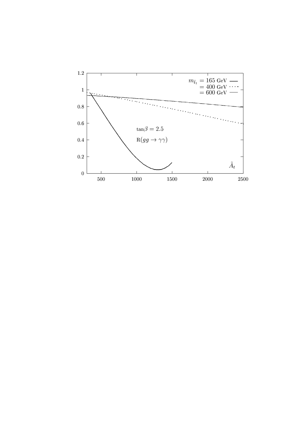
Figure 2: SUSY loop effects on R$(gg\rightarrow\gamma\gamma)$ as a function of $\tilde{A}_{t}$ for $\mbox{tg}\beta=2.5$ and $m_{\tilde{t}_{1}}=165,400$ and 600 GeV.

Figs. 1–3 show the deviations from their SM values of the partial decay widths of the $h$ boson into two photons and two gluons as well as their product which gives the cross section times branching ratio $\sigma(gg\rightarrow h\rightarrow\gamma\gamma)$. The quantities $R$ are defined as the partial widths including the SUSY loop contributions [all charged SUSY particles for $h\rightarrow\gamma\gamma$ and squark loops for $h\rightarrow gg$] normalized to the partial decay widths without the SUSY contributions, which in the decoupling limit correspond to the SM contributions: $R=\Gamma_{\rm MSSM}/\Gamma_{\rm SM}$.

Since, as discussed previously, the main SUSY contribution for small values of $\mbox{tg}\beta$ are due to $\tilde{t}$ loops, the loop contributions are shown in Figs. 1–2 as a function of $\tilde{A}_{t}$ for $\mbox{tg}\beta=2.5$ and the values $m_{\tilde{t}_{1}}=200$ GeV (Fig. 1) and $m_{\tilde{t}_{1}}=165,400$ and 600 GeV (Fig. 2) for the $\tilde{t}_{1}$ mass [which then fixes the parameters $m_{\tilde{t}_{L}}\simeq m_{\tilde{t}_{R}}\simeq m_{\tilde{q}}$]. The other parameters are chosen as $M_{2}=-\mu=250$ and 500 GeV for the scenarii $m_{\tilde{t}_{1}}\leq 200$ GeV and $>200$ GeV respectively; the choice of these two different values is motivated by the requirement that the lightest neutralino must be lighter than $\tilde{t}_{1}$ in each scenario.

Concentrating first on the case $m_{\tilde{t}_{1}}=200$ GeV, for small values of $\tilde{A}_{t}$ there is no mixing in the stop sector and the dominant component of the $h\tilde{t}\tilde{t}$ couplings, eq. (2), is the one proportional to $m_{t}^{2}/M_{Z}^{2}$ [here, both $\tilde{t}_{1}$ and $\tilde{t}_{2}$ contribute since their masses and couplings to $h$ are almost the same]. The sign of this component, compared to the $ht\bar{t}$ coupling, is such that the top and stop contributions interfere constructively in the $hgg$ and $h\gamma\gamma$ amplitudes. This leads to an enhancement of the $h\rightarrow gg$ decay width up to $60\%$ in the MSSM. However, the $h\rightarrow\gamma\gamma$ decay width is dominated by the $W$ amplitude which interferes destructively with the top and stop quark amplitudes [there is also a small contribution from chargino loops in this scenario since the $\chi_{1}^{+}$ mass is $\simeq 230$ GeV] and the $\tilde{t}$ contributions reduce the $h\rightarrow\gamma\gamma$ decay width by an amount up to $-20\%$. The product R($gg\rightarrow\gamma\gamma$) in the MSSM is then enhanced by a factor $\sim 1.2$ in this case.

With increasing $\tilde{A}_{t}$, the two components of the $h\tilde{t}_{1}\tilde{t}_{1}$ coupling [which have opposite sign because $\sin 2\theta_{\tilde{t}}\propto m_{t}\tilde{A}_{t}$ in eq. (2)] interfere destructively and partly cancel each other, resulting in a rather small stop contribution. For a value $\tilde{A}_{t}\sim 400$ GeV, $g_{h\tilde{t}_{1}\tilde{t}_{1}}\sim 0$ and the $\tilde{t}_{1}$ contributions to the $hgg$ and $h\gamma\gamma$ amplitudes vanish [here, $\tilde{t}_{2}$ is too heavy to contribute]. For larger values of $\tilde{A}_{t}$, the second component of the $h\tilde{t}_{1}\tilde{t}_{1}$ coupling becomes the most important one, and the $\tilde{t}_{1}$ loop contribution [$\tilde{t}_{2}$ is too heavy to contribute] interferes destructively with the one of the top quark. This leads to an enhancement of R$(h\rightarrow\gamma\gamma)$ and a reduction of R$(gg\rightarrow h)$. However, the reduction of the latter is much stronger than the enhancement of the former [recall that the $W$ contribution in the $h\rightarrow\gamma\gamma$ decay is much larger than the top contribution] and the product R($gg\rightarrow\gamma\gamma$) decreases with increasing $\tilde{A}_{t}$. For $\tilde{A}_{t}$ values of about 1.5 TeV, the signal for $gg\rightarrow h\rightarrow\gamma\gamma$ in the MSSM is smaller by a factor of $\sim 5$ compared to the SM case.

Fig. 2 shows the deviation R$(gg\rightarrow\gamma\gamma)$ with the same parameters as in Fig. 1 but with different $\tilde{t}_{1}$ masses, $m_{\tilde{t}_{1}}=165,400$ and 600 GeV, and to ensure an LSP lighter than $\tilde{t}_{1}$, with $M_{2}=-\mu=500$ GeV for $m_{\tilde{t}_{1}}\geq 400$ GeV. For larger masses, the top squark contribution $\propto 1/m_{\tilde{t}_{1}}^{2}$, will be smaller than in the previous case. In the no–mixing case, the enhancement (reduction) of the $hgg(h\gamma\gamma)$ amplitude is only of the order of 10% for $m_{\tilde{t}_{1}}\simeq 400$ GeV, and leads to an almost constant cross section times branching ratio for the $gg\rightarrow h\rightarrow\gamma\gamma$ process compared to the SM case. Again the stop contribution vanishes for some intermediate value of $\tilde{A}_{t}$, and then increases again in absolute value for larger $\tilde{A}_{t}$. However, for $m_{\tilde{t}_{1}}\simeq 400$ GeV, the effect is less striking compared to the case of $m_{\tilde{t}_{1}}=200$ GeV, since here $\sigma(gg\rightarrow h)\times{\rm BR}(h\rightarrow\gamma\gamma$) drops by less than a factor of 2, even for extreme values of $\tilde{A}_{t}\sim 2.5$ TeV. As expected, the effect of the top squark loops will become less important if the $\tilde{t}_{1}$ mass is increased further to 600 GeV for instance. In contrast, if the stop mass is reduced to $m_{\tilde{t}_{1}}\simeq 165$ GeV, the drop in R$(gg\rightarrow\gamma\gamma)$ will be even more important: for $\tilde{A}_{t}\sim 1.5$ TeV, the $gg\rightarrow\gamma\gamma$ cross section times branching ratio including stop loops is an order of magnitude smaller than in the SM. For $\tilde{A}_{t}\sim 1.3$ TeV, the stop amplitude almost cancels completely the top and bottom quark amplitudes; the non–zero value of R$(gg\rightarrow\gamma\gamma)$ is then due to the imaginary part of the bottom quark contribution.

Note that $M_{h}$ varies with $\tilde{A}_{t}$, and no constraint on $M_{h}$ has been set in Figs. 1–2. Requiring $M_{h}\raisebox{-3.69899pt}{~{}\shortstack{$>$ \\ [-0.07cm] $\sim$}}~{}90$ GeV, the lower range $\tilde{A}_{t}\raisebox{-3.69899pt}{~{}\shortstack{$<$ \\ [-0.07cm] $\sim$}}~{}350$ GeV and the upper ranges $\tilde{A}_{t}\raisebox{-3.69899pt}{~{}\shortstack{$>$ \\ [-0.07cm] $\sim$}}~{}1.5(2.3)$ TeV for $m_{\tilde{t}_{1}}=200(400)$ GeV for instance, are ruled out. [This is due to the fact that the maximal value of $M_{h}$ for a given $\mbox{tg}\beta$ and a common scalar mass $m_{\tilde{q}}$, which here is fixed in terms of $m_{\tilde{t}_{1}},\mbox{tg}\beta$ and $\tilde{A}_{t}$, the $h$ boson mass increases with increasing $\tilde{A}_{t}$ and reaches a maximal value for $\tilde{A}_{t}\simeq\sqrt{6}m_{\tilde{q}}$; when $\tilde{A}_{t}$ exceeds this value, the maximal value of the $h$ boson mass will start decreasing.] This means that the scenario where R$(gg\rightarrow\gamma\gamma)>1$, which occurs only for small values of $\tilde{A}_{t}\raisebox{-3.69899pt}{~{}\shortstack{$<$ \\ [-0.07cm] $\sim$}}~{}300$ GeV for $m_{\tilde{t}_{1}}=200$ GeV is ruled out for $M_{h}\raisebox{-3.69899pt}{~{}\shortstack{$>$ \\ [-0.07cm] $\sim$}}~{}90$ GeV. Therefore, if this constraint is implemented, the cross section times branching ratio for the $gg\rightarrow\gamma\gamma$ process in the MSSM will always be smaller than in the SM case, making more delicate the search for the $h$ boson at the LHC with this process.

Let me turn now to the case of $\mbox{tg}\beta\gg 1$, where the off–diagonal entry in the $\tilde{b}$ mass matrix will play a major role. For instance, choosing moderate values for the universal trilinear coupling $A\equiv A_{t}=A_{b}$ and the common soft–SUSY breaking scalar mass, a large value of the parameter $\mu$ [which is then multiplied by $\mbox{tg}\beta$] will make the off–diagonal entry very large, leading to a sizeable splitting between the two sbottom masses with $m_{\tilde{b}_{1}}$ possibly rather small, and a large $g_{h\tilde{b}_{1}\tilde{b}_{1}}$ coupling which could generate large $\tilde{b}_{1}$ loop contributions to the $hgg$ and $h\gamma\gamma$ vertices. This is shown in Fig. 3, where the effect of the $\tilde{t}$ and $\tilde{b}$ loops [for $h\rightarrow\gamma\gamma$ a small contribution is also coming from chargino loops] on the quantities R$(h\rightarrow\gamma\gamma)$ and R$(gg\rightarrow h\rightarrow\gamma\gamma)$ is displayed as a function of $\mu$ [with $\mu<0$] for $\mbox{tg}\beta=50$. The values $m_{\tilde{b}_{1}}=200$ GeV and $M_{2}=300$ GeV have been chosen. The thick and thin curves correspond to the two choices $A\equiv\tilde{A}_{t}=\tilde{A}_{b}=0$ and 0.5 TeV, respectively.

The effects of SUSY loops on the $h\rightarrow\gamma\gamma$ decay width is relatively small, barely exceeding the level of 10%. In turn, the deviations of the R$(h\rightarrow gg)$ and thus R$(gg\rightarrow h\rightarrow\gamma\gamma$) observables from unity are substantial for large values of $|\mu|$, exceeding a factor of 2 for $|\mu|\sim 800$ GeV. For this $|\mu|$ value and above, only the $\tilde{b}$ contribution is sizeable: the $\tilde{t}_{1}$ is either too heavy, or its couplings to the $h$ boson small [this explains why the two curves for $A=0$ and 0.5 TeV are almost the same]. For lower $\mu$ values, the difference between the two curves is due to the $\tilde{t}_{1}$ contribution. Thus the effect of sbottom loops on the observable R$(gg\rightarrow\gamma\gamma$) can be sizeable for large values of $|\mu|$. For extreme values, $|\mu|\simeq 1.2$ TeV [for larger values of $|\mu|$ the $h$ boson mass becomes smaller than $90$ GeV], the $gg\rightarrow\gamma\gamma$ cross section in the MSSM can be suppressed compared to the SM case by a factor of 5. Of course, if the $\tilde{b}_{1}$ mass is increased (reduced) the effect becomes less (more) striking.

Finally, a remark on the situation where the decoupling limit is not yet reached is in order. In this case the $hWW$ and $htt$ couplings are smaller than in the SM, and both the $gg\rightarrow h$ cross section and $h\rightarrow\gamma\gamma$ widths are suppressed compared to the SM case, even in the absence of the squark loops. Including light $\tilde{t}$ squark contributions will further decrease the amplitudes in the case of large $\tilde{A}_{t}$ as shown in Fig. 4 for $\mbox{tg}\beta=2.5$ and $M_{A}=200$ GeV. For large values of $\mbox{tg}\beta$, the $hgg$ amplitude can be enhanced by the $b$–loop contribution, but the $h\rightarrow\gamma\gamma$ branching ratio is strongly suppressed due to the absence of the $W$–loop and the increase of the total decay width $\propto m_{b}^{2}\tan^{2}\beta$. In the case of the heavy CP–even Higgs boson $H$, squark loop contributions to the cross section $gg\rightarrow H$ can be even larger since because of the larger value of $M_{H}$, more room will be left for the $\tilde{t}$ and $\tilde{b}$ squarks before they decouple form the $Hgg$ amplitude. In addition, for $M_{H}$ values above the squark pair threshold, the decays $H\rightarrow\tilde{t}_{1}\tilde{t}_{1}$ or $H\rightarrow\tilde{b}_{1}\tilde{b}_{1}$ will be kinematically allowed and could have large branching ratios, therefore suppressing the other decay modes including the $H\rightarrow\gamma\gamma$ channel. For the pseudoscalar Higgs boson, however, squark loops will not have drastic effects on the production cross section $\sigma(gg\rightarrow A)$: because of CP–invariance, the $A$ boson couples only to $\tilde{t}_{1}\tilde{t}_{2}$ or $\tilde{b}_{1}\tilde{b}_{2}$ pairs while the gluon coupling to different squarks is absent; the $Agg$ amplitude, therefore, cannot be built at lowest order by scalar quark loops.

4. Conclusions

I discussed the effects of $\tilde{t}$ and $\tilde{b}$ squarks on the main production mechanism of the lightest neutral SUSY Higgs boson $h$ at the LHC, $gg\rightarrow h$, and on the important decay channel $h\rightarrow\gamma\gamma$ in the context of the MSSM. If the off–diagonal entries in the $\tilde{t}$ and $\tilde{b}$ mass matrices are large, the eigenstates $\tilde{t}_{1}$ and $\tilde{b}_{1}$ can be rather light and at the same time their couplings to the $h$ boson strongly enhanced. The cross section times branching ratio $\sigma(gg\rightarrow h)\times{\rm BR}(h\rightarrow\gamma\gamma)$ can be then much smaller than in the SM, even in the decoupling regime, $M_{A}\gg M_{Z}$, where the $h$–boson has SM–like couplings to fermions and gauge bosons. Far from this decoupling limit, the cross section times branching ratio is further reduced in general due to the additional suppression of the $ht\bar{t}$ and $hWW$ couplings.

Acknoweldgements:
I thank Daniel Denegri and Francois Richard for stimulating and fruitful discussions.

Figure 1: SUSY loop effects on R$(h\rightarrow\gamma\gamma)$, R$(gg\rightarrow h)$ and their product R$(gg\rightarrow\gamma\gamma)$ as a function of $\tilde{A}_{t}$ for $\mbox{tg}\beta=2.5$ and $m_{\tilde{t}_{1}}=200$ GeV; $M_{2}=-\mu=250$ GeV.

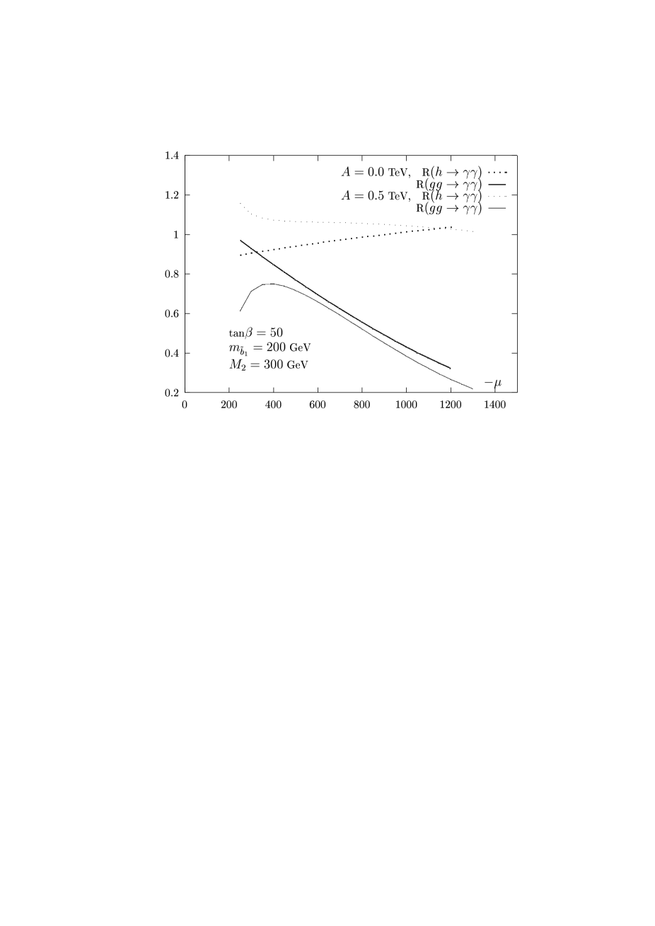
Figure 3: SUSY loop effects on R$(h\rightarrow\gamma\gamma)$ and R$(gg\rightarrow h\rightarrow\gamma\gamma)$ as a function of $-\mu$ for $\mbox{tg}\beta=50$ and $m_{\tilde{b}_{1}}=200$ GeV and $A\equiv\tilde{A}_{t}=\tilde{A}_{b}=0(0.5)$ TeV for the thick (thin) curves.

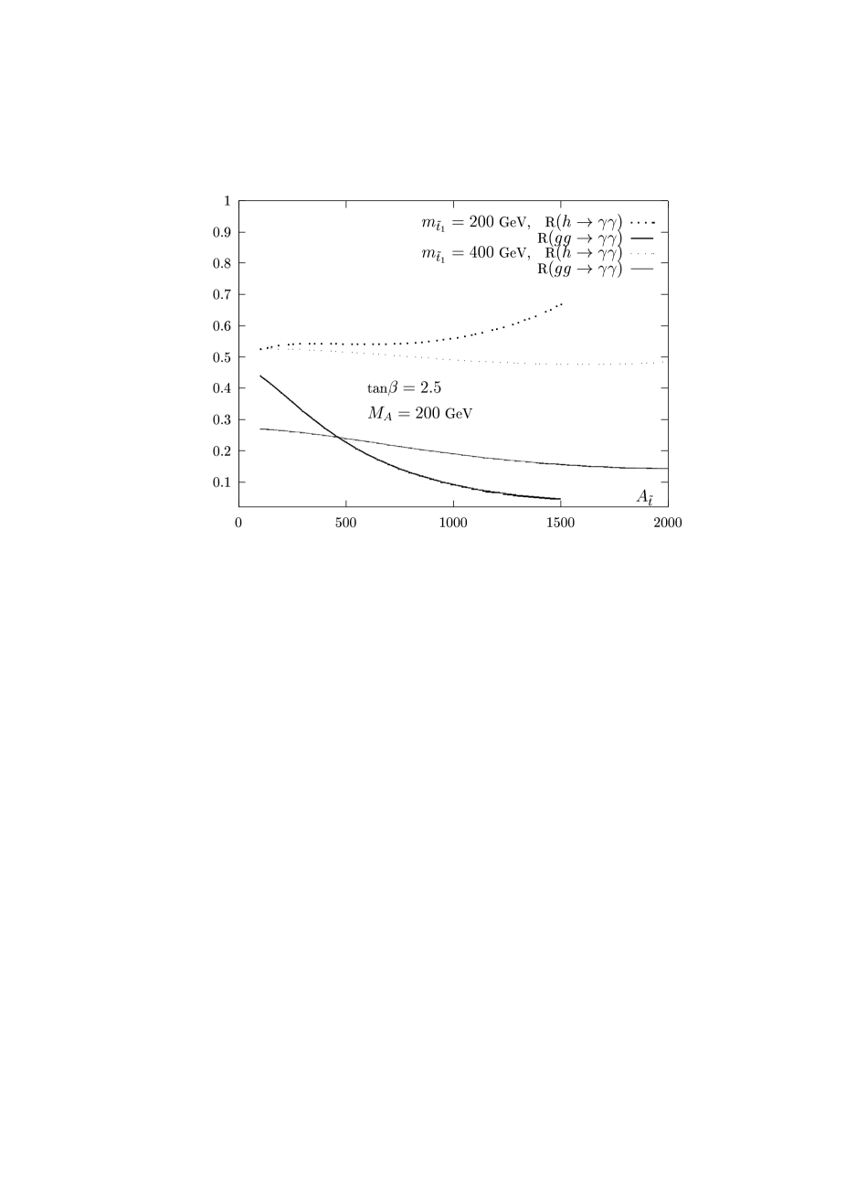
Figure 4: SUSY loop effects on R$(h\rightarrow\gamma\gamma)$ and R$(gg\rightarrow h\rightarrow\gamma\gamma)$ as a function of $\tilde{A}_{t}$ for $\mbox{tg}\beta=2.5,M_{A}=200$ GeV and two values $m_{\tilde{t}_{1}}=200$ and 400 GeV.

References

- [1] For reviews see: P. Fayet and S. Ferrara, Phys. Rep. 32 (1997) 249; H.P. Nilles, Phys. Rep. 110, 1 (1984); H.E. Haber and G.L. Kane, Phys. Rep. 117, 75 (1985).
- [2] For a review, see: J.F. Gunion, H.E. Haber, G.L. Kane and S. Dawson, “The Higgs Hunters Guide”, Addison–Wesley, Reading 1990.
- [3] H.E. Haber, CERN-TH/95-109 and hep-ph/9505240.
- [4] Particle Data Group, Phys. Rev. D54, 1 (1996); for a recent collection of data, see P. Janot, CEFIPRA Indo–French meeting, Mumbai 1997.
- [5] Y. Okada, M. Yamaguchi and T. Yanagida, Prog. Theor. Phys. 85 (1991) 1; H. Haber and R. Hempfling, Phys. Rev. Lett. 66 (1991) 1815; J. Ellis, G. Ridolfi and F. Zwirner, Phys. Lett. 257B (1991) 83; R. Barbieri, F. Caravaglios and M. Frigeni, Phys. Lett. 258B (1991) 167; M. Carena, M. Quiros and C.E.M. Wagner, Nucl. Phys. B461 (1996) 407; H. Haber, R. Hempfling and A. Hoang, Z. Phys. C75 (1997) 539.
- [6] For a recent review on Higgs physics at the LHC, see e.g.: J.F. Gunion et al., hep-ph/9602238, Proceedings of the Snowmass 96 Workshop.
- [7] J. Ellis, M. Gaillard and D. Nanopoulos, Nucl. Phys. B106 (1976) 292; A. I. Vainshtein et al., Sov. J. Nucl. Phys. 30 (1979) 711; J.F. Gunion and H.E. Haber, Phys. Rev. D48 (1993) 5109; G. L. Kane, G. D. Kribs, S. P. Martin and J. D. Wells, Phys. Rev. D53 (1996) 213; B. Kileng, P. Osland and P.N. Pandita, Z. Phys. C71 (1996) 87.
- [8] H. Georgi et al., Phys. Rev. Lett. 40 (1978) 692.
- [9] A. Djouadi, M. Spira and P.M. Zerwas, Phys. Lett. B264 (1991) 440; S. Dawson, Nucl. Phys. B359 (1991) 283; M. Spira et al., Nucl. Phys. B453 (1995) 17; S. Dawson, A. Djouadi and M. Spira, Phys. Rev. Lett. 77 (1996) 16.
- [10] ATLAS Collaboration, Technical Proposal, Report CERN–LHCC 94–43; CMS Collaboration, Technical Proposal, Report CERN–LHCC 94–38.
- [11] A. Djouadi, V. Driesen, W. Hollik and J.I. Illana, Eur. Phys. J. C1 (1998) 149.
- [12] M. Drees, M. Guchait and P. Roy, Phys. Rev. Lett. 80 (1998) 2047.
- [13] A. Djouadi, J. Kalinowski and M. Spira, Comput. Phys. Commun. 108 (1998) 56.
- [14] See for instance, G. Altarelli, hep-ph/9611239.
- [15] A. Djouadi, J.L. Kneur and G. Moultaka, Phys. Rev. Lett. 80 (1998) 1830.