Next-to-leading order calculation of four-jet observables in electron-positron annihilation

Abstract

The production of four jets in electron-positron annihilation allows for measuring the strong coupling and the underlying group structure of the strong interaction simultaneously. This requires next-to-leading order perturbative prediction for four-jet observables. In this paper we describe the theoretical formalism of such a calculation with sufficient details. We use the dipole method to construct a Monte Carlo program that can be used for calculating any four-jet observable at the next-to-leading order accuracy. As new results, we present the next-to-leading order prediction for the thrust minor, $y_{4}$ and C parameter (at C $\geq$ 0.75) four-jet shape variables and the four-jet rates with the Cambridge jet clustering algorithm.

]

I Introduction

Electron-positron annihilation into hadrons is the cleanest process to test Quantum Chromodynamics (QCD) [1] in high energy elementary particle reactions. In this process the initial state is completely known and there is a lot of quantities, for instance the total cross section and jet related correlations, that depend on the long distance properties of the theory very little. These quantities can be calculated in perturbative QCD as a function of a single parameter, the strong coupling. For this reason the various QCD tests at electron-positron colliders [2, 3, 4, 5, 6, 7] can be regarded as experiments for determining ${\alpha_{s}}$.

The other ingredient of QCD, that is in principle free, is the underlying gauge group. Although by now nobody questions that QCD is based upon SU(3) gauge theory, the “full” measurement of QCD, that is the simultaneous measurement of the strong coupling and the eigenvalues of the quadratic Casimirs of the underlying gauge theory, the $C_{F}$ and $C_{A}$ color charges, is not a purely academic exercise. The possible existence of light gluinos [8] influences both the value of ${\alpha_{s}}$ and the measured value of the color charges (or, assuming SU(3)_c, the value of the light fermionic degrees of freedom ${N_{\rm f}}$). Thus the only consistent framework to check whether the data favor or exclude the additional degrees of freedom is a simultaneous fit of these parameters to data.

In principle any observable depends on these basic parameters. The sensitivity of a given observable on the color charges however, is influenced by the fact that in perturbation theory the three gluon coupling appears at tree level first for four-jet final states. In the total cross section and for three-jet like quantities the adjoint color charge appears only in the radiative corrections. Therefore, four-jet observables seem to be the best candidates to measure the color factors. Indeed, during the first phase of operation of the Large Electron Positron Collider (LEP) four-jet events were primarily used for measuring $C_{F}$ and $C_{A}$ [9].These measurements however, were not complete in the sense mentioned above. The lack of knowledge about the perturbative prediction for four-jet observables at O($\alpha_{s}^{3}$) prevented the experimental collaborations from fixing the absolute normalization of the perturbative prediction, therefore, ${\alpha_{s}}$ could not be measured using the same observables.

Recently the next-to-leading order corrections to various four-jet observables have been calculated [10, 11, 12, 13, 14, 15, 16]. In this article we give sufficient details of our work [13, 14, 15] and present several new results for next-to-leading order predictions of four-jet observables that were not published before. The important development that made possible these calculations was that the one-loop amplitudes for the relevant QCD subprocesses, i.e. for $e^{+}e^{-}\to$ 4 partons, became available. In Refs. [17, 18] Campbell, Glover and Miller introduced FORTRAN programs that calculate the next-to-leading order squared matrix elements of the $e^{+}e^{-}\to\gamma^{*}\to{\bar{q}}q{\bar{Q}}Q$ and ${\bar{q}}qgg$ processes. In Refs. [19, 20] Bern, Dixon, Kosower and Wienzierl gave analytic formulas for the helicity amplitudes of the same processes with the $e^{+}e^{-}\to Z^{0}\to$ 4 partons channel included as well. For the sake of completeness, in our work we use the amplitudes of Refs. [20] for the loop corrections. Although the tree-level helicity amplitudes for the $e^{+}e^{-}\to$ 5 partons subprocesses had been known [21], we calculated them anew and present the results in this article in terms of Weyl spinors conforming with the notation used for describing the one-loop helicity amplitudes [20]. We also present the previously unpublished color linked helicity dependent Born matrix elements for the $e^{+}e^{-}\to$ 4 partons processes, which are needed also for the next-to-leading order calculation of the three-jet production in deep inelastic scattering and for vector boson plus two-jet production in hadron collisions.

In Sec. II we give details of the analytical and numerical calculation and describe how we parametrise our results. In Sec. III we present the complete O($\alpha_{s}^{3}$) predictions for the four-jet rates using the Durham algorithm [22] and the Cambridge algorithm proposed recently [23] and make a comparison of these algorithms from the perturbation theory point of view. We show the next-to-leading order results for the shape variables thrust minor and $y_{4}$ often used in experimental analyses and for the C parameter distribution at C $\geq$ 0.75. Sec. IV contains our conclusions. We present analytic results for the four- and five-parton tree-level helicity amplitudes in Appendix A, and perform the color summation in Appendix B.

II Details of the calculation

A Cancellation of infrared divergences

It is well-known that the next-to-leading order correction is a sum of two integrals,

$$\sigma^{\rm NLO}\equiv\int{\rm d}\sigma^{\rm NLO}=\int_{5}{\rm d}\sigma^{\rm R}+\int_{4}{\rm d}\sigma^{\rm V}\>,$$ (1)

where ${\rm d}\sigma^{\rm R}$ is an exclusive cross section of five partons in the final state:

$$\int_{5}{\rm d}\sigma^{\rm R}=\int{\rm d}\Gamma^{(5)}<|{\cal M}_{5}^{\rm tree}|^{2}>J_{5}\>,$$ (2)

and ${\rm d}\sigma^{\rm V}$ is the one-loop correction to the process with four partons in the final state:

$$\int_{4}{\rm d}\sigma^{\rm V}=\int{\rm d}\Gamma^{(4)}<|{\cal M}_{4}^{\rm 1-loop}|^{2}>J_{4}\>,$$ (3)

— the real and virtual corrections. Although we specify our formulas to the case of four-jet calculation, one can use the formulas of this section to obtain the $m$-jet cross section by simply changing 4 (5) to $m\;(m+1)$.

The two integrals on the right-hand side of Eq. (1) are separately divergent in $d=4$ dimensions, but their sum is finite provided the jet function $J_{n}$ defines an infrared safe quantity, which formally means that

$$J_{5}\to J_{4}$$ (4)

in any case, where the five-parton and the four-parton configurations are kinematically degenerate. The presence of singularities means that the separate pieces have to be regularized, and the divergences have to be cancelled. We use dimensional regularization in $d=4-2{\varepsilon}$ dimensions [24], in which case the divergences are replaced by double and single poles in ${\varepsilon}$. We assume that ultraviolet renormalization of all Green functions to one-loop order has been carried out, so the poles are of infrared origin. In order to obtain the finite sum, we use a slightly modified version of the dipole method of Catani and Seymour [25] that exposes the cancellation of the infrared singularities directly at the integrand level.

The reason for modifying the original dipole formalism is numerical. The essence of the dipole method is to define a single subtraction term ${\rm d}\sigma^{\rm A}$ — the dipole subtraction —, that reguralizes the real correction in all of its singular (soft and collinear) limits. Thus, the two singular integrals in Eq. (1) are substituted by two finite ones:

$$\sigma^{\rm NLO}=\int_{5}{\rm d}\sigma_{5}^{\rm NLO}+\int_{4}{\rm d}\sigma_{4}^{\rm NLO}\>,$$ (5)

where

$$\int_{5}{\rm d}\sigma_{5}^{\rm NLO}=\int_{5}\left[{\rm d}\sigma^{\rm R}-{\rm d}\sigma^{\rm A}\right]$$ (6)

and

$$\int_{4}{\rm d}\sigma_{4}^{\rm NLO}=\int_{4}\left[{\rm d}\sigma^{\rm V}+\int_{1}{\rm d}\sigma^{\rm A}\right]$$ (7)

There are many ways to define the subtraction term, but all must lead to the same finite next-to-leading order correction. Since the virtual correction is not positive definite, then depending on the size of the subtraction term it may happen that either ${\rm d}\sigma_{5}^{\rm NLO}$ or ${\rm d}\sigma_{4}^{\rm NLO}$ is not positive definite. From numerical point of view the best situation is when both are positive definite, so that numerical cancellation of terms with opposite sign does not occur. We define the subtraction term as a function of a parameter $\alpha\in(0,1]$ which essentially controls the region of the five-parton phase space over which the subtraction is non-zero such that $\alpha=1$ means the full dipole subtraction (see subsection II.B). By tuning the value of $\alpha$, we can achieve that we add two positive definite integrals for almost all values of the observable to obtain the full correction. We use an $\alpha\simeq 0.1$, which is advantageous also for saving CPU time: The large number of dipole terms and their somewhat complicated analytic structure makes the evaluation of the subtraction term rather time consuming. Constraining the phase space over which the subtraction is zero we can speed up the program.

In spite that the five-parton integral in Eq. (6) is finite, we introduce a very small cutoff in the phase space around the singular regions. Such a cutoff does not alter the value of the integral, but helps avoiding the cancellation of very large numbers that could lead to arbitrary values close to the singularity due to the finite machine precision. This cutoff is useful, but is also dangerous: if the subtraction is not correct, the five-parton integral becomes finite, but incorrect. The third advantage of using the parameter $\alpha$ is that such errors can be spotted by varying the value of $\alpha$ and checking whether the full correction is independent of this parameter.

B Dipole formulas for final state singularities

In this subsection we recall those dipole factorization formulas that are relevant to our calculation. We do this only to the extent that we can define the simple modification to the original formalism and the explicit cross section formulas of our calculation unambiguously. For further details we refer to the original work of Catani and Seymour [25].

In the dipole method the subtraction term is a sum of several dipole terms,

$$\int_{5}{\rm d}\sigma^{\rm A}=\sum_{k\neq i,j}\int\!{\rm d}\Gamma^{(5)}\,{\cal D}_{ij,k}\,J_{4}\>,$$ (8)

where the dipole ${\cal D}_{ij,k}$ is a function of the final state momenta $p_{l}$ and is given by

$${\cal D}_{ij,k}(p_{1},\ldots,p_{5})=-\frac{1}{2p_{i}\cdot p_{j}}$$ (9)

$$\;\times{}_{4}\langle{\ldots,{\widetilde{ij}},\ldots,{\widetilde{k}},\ldots}|\,\frac{{{\mbox{\boldmath$T$}}}_{k}\cdot{{\mbox{\boldmath$T$}}}_{ij}}{{{\mbox{\boldmath$T$}}}_{ij}^{2}}\;{{\mbox{\boldmath$V$}}}_{ij,k}\,|{\ldots,{\widetilde{ij}},\ldots,{\widetilde{k}},\ldots}\rangle_{4}\>.$$ (10)

In Eq. (9) $|{\ldots,{\widetilde{ij}},\ldots,{\widetilde{k}},\ldots}\rangle_{4}$ is a vector in color + helicity space defining the four-parton amplitude obtained from the original five-parton Born amplitude by replacing $a)$ the partons $i$ and $j$ with a single parton ${\widetilde{ij}}$ (the emitter) and $b)$ the parton $k$ with the parton $\widetilde{k}$ (the spectator). The momenta of the spectator and the emitter are given in terms of a dimensionless variable

$$y_{ij,k}=\frac{p_{i}p_{j}}{p_{i}p_{j}+p_{j}p_{k}+p_{k}p_{i}}\>,$$ (11)

as

$${\widetilde{p}}_{k}^{\mu}=\frac{1}{1-y_{ij,k}}\,p_{k}^{\mu}\>,\quad{\widetilde{p}}_{ij}^{\mu}=p_{i}^{\mu}+p_{j}^{\mu}-\frac{y_{ij,k}}{1-y_{ij,k}}\,p_{k}^{\mu}\>.$$ (12)

${{\mbox{\boldmath$T$}}}_{k}$ and ${{\mbox{\boldmath$T$}}}_{ij}$ are the color charges of the spectator and the emitter. These color charges are defined by their action onto the color space: If particle $i$ emits a gluon with color index $c$ then the color-charge operator ${{\mbox{\boldmath$T$}}}_{i}$ has the following matrix element in color space

$$\langle{c_{1},\ldots,c_{i},\ldots,c_{4},c}|{{\mbox{\boldmath$T$}}}_{i}|{b_{1},\ldots,b_{i},\ldots,b_{4}}\rangle=$$ (13)

$$\qquad\qquad\delta_{c_{1}b_{1}}\ldots T_{c_{i}b_{i}}^{c}\ldots\delta_{c_{4}b_{4}}\>,$$ (14)

where $T_{c_{i}b_{i}}^{c}\equiv F_{c_{i}b_{i}}^{c}=-{\rm i}f_{cc_{i}b_{i}}$ (color-charge matrix in the adjoint representation) if the emitting particle $i$ is a gluon and $T_{c_{i}b_{i}}^{c}\equiv t^{c}_{c_{i}b_{i}}$ (color-charge matrix in the fundamental representation) if the emitting particle $i$ is a quark (in the case of an antiquark emitter $T_{c_{i}b_{i}}^{c}\equiv{\bar{t}}^{c}_{c_{i}b_{i}}=-t^{c}_{b_{i}c_{i}}$).

In Eq. (9) the splitting matrices, ${{\mbox{\boldmath$V$}}}_{ij,k}$ are matrices in the helicity space of the emitter. They depend on the kinematic variables $y_{ij,k}$ and

$${\tilde{z}}_{i}=\frac{p_{i}{\widetilde{p}}_{k}}{{\widetilde{p}}_{ij}{\widetilde{p}}_{k}}$$ (15)

and take different forms for the splitting of different partons (see Eqs. (5.7–5.9) in Ref. [25]).

The definition of the dipole momenta makes possible the exact factorization of the five-particle phase space into a four-particle and a one-particle phase space

$${\rm d}\Gamma^{(5)}(p_{1},\ldots,p_{5})=$$ (16)

$$\qquad{\rm d}\Gamma^{(4)}(\ldots,{\widetilde{p}}_{ij},\ldots,{\widetilde{p}}_{k},\ldots)\,\left[{\rm d}p_{i}({\widetilde{p}}_{ij},{\widetilde{p}}_{k})\right]\>,$$ (17)

where

$$\left[{\rm d}p_{i}({\widetilde{p}}_{ij},{\widetilde{p}}_{k})\right]=\frac{{\rm d}^{d}p_{i}}{(2\pi)^{d-1}}\,\delta_{+}(p_{i}^{2})\,{\cal J}(p_{i};{\widetilde{p}}_{ij},{\widetilde{p}}_{k})\>,$$ (18)

and the Jacobian factor is

$${\cal J}(p_{i};{\widetilde{p}}_{ij},{\widetilde{p}}_{k})=\Theta(1-{\tilde{z}}_{i})\,\Theta(1-y_{ij,k})\,\frac{(1-y_{ij,k})^{d-3}}{1-{\tilde{z}}_{i}}\>.$$ (19)

As mentioned before, we modify the original formalism such that we constrain the phase space over which the dipoles are subtracted:

$$\int_{5}{\rm d}\sigma^{\rm A}(\alpha)=\sum_{k\neq i,j}\int\!{\rm d}\Gamma^{(5)}\>{\cal D}_{ij,k}\>\Theta(y_{ij,k}<\alpha)\>J_{4}\>,$$ (20)

with $\alpha\in(0,1]$. The jet function in Eq. (20) is a four-parton jet function that depends on the momenta ${\widetilde{p}}_{ij}$ and ${\widetilde{p}}_{k}$, but not on $p_{i}$, therefore, the integral over the one-parton phase space can be performed analytically. It can be shown that after integration of the dipole ${\cal D}_{ij,k}(p_{1},\ldots,p_{5})$ over $[{\rm d}p_{i}({\widetilde{p}}_{ij},{\widetilde{p}}_{k})]$, only color correlations survive [25], in the form:

$$\int\!\left[{\rm d}p_{i}({\widetilde{p}}_{ij},{\widetilde{p}}_{k})\right]\,{\cal D}_{ij,k}(p_{1},\ldots,p_{5})\,\Theta(y_{ij,k}<\alpha)=$$ (21)

$$\qquad\qquad-\,{\cal V}_{ij,k}(\alpha)\>\frac{1}{{{\mbox{\boldmath$T$}}}_{ij}^{2}}\left|{\cal M}^{ij,k}_{4}(\ldots,{\widetilde{ij}},\ldots,{\widetilde{k}},\ldots)\right|^{2}\>,$$ (22)

where

$$\left|{\cal M}^{i,j}_{4}(1,\ldots,4)\right|^{2}={}_{4}\langle{1,\ldots,4}|\,{{\mbox{\boldmath$T$}}}_{i}\cdot{{\mbox{\boldmath$T$}}}_{j}\,|{1,\ldots,4}\rangle_{4}$$ (23)

are the color-correlated four-parton tree matrix elements. Their explicit expressions are given in Appendix B. In Eq. (21)

$${\cal V}_{ij,k}(\alpha)=$$ (24)

$$\quad\int\!\left[{\rm d}p_{i}({\widetilde{p}}_{ij},{\widetilde{p}}_{k})\right]\,\Theta(y_{ij,k}<\alpha)\,\frac{1}{2p_{i}\cdot p_{j}}\;<{{\mbox{\boldmath$V$}}}_{ij,k}>\,\equiv$$ (25)

$$\quad\frac{{\alpha_{s}}}{2\pi}\frac{1}{\Gamma(1-{\varepsilon})}\left(\frac{4\pi\mu^{2}}{2{\widetilde{p}}_{ij}{\widetilde{p}}_{k}}\right)^{{\varepsilon}}{\cal V}_{ij}({\varepsilon},\alpha)\;,$$ (26)

where $<{{\mbox{\boldmath$V$}}}_{ij,k}>$ denotes the average of ${{\mbox{\boldmath$V$}}}_{ij,k}$ over the polarisations of the emitter parton ${\widetilde{ij}}$. The functions ${\cal V}_{ij}({\varepsilon},\alpha)$ depend only on the flavour indices $i$ and $j$. Rewriting the one-particle phase space in terms of the kinematic variables ${\tilde{z}}_{i}$ and $y$, from the definition of ${\cal V}_{ij}({\varepsilon},\alpha)$ in Eq. (24) we obtain [

$${\cal V}_{ij}({\varepsilon},\alpha)=\int_{0}^{1}\!{\rm d}{\tilde{z}}_{i}\,\left({\tilde{z}}_{i}(1-{\tilde{z}}_{i})\right)^{-{\varepsilon}}\int_{0}^{\alpha}\!{\rm d}y\,y^{-1-{\varepsilon}}\left(1-y\right)^{1-2{\varepsilon}}\;\frac{<{{\mbox{\boldmath$V$}}}_{ij,k}({\tilde{z}}_{i};y)>}{8{\pi}{\alpha_{s}}\mu^{2{\varepsilon}}}\;,$$ (27)

where the spin-averaged splitting functions are given in Eqs. (5.29-5.31) of Ref. [25]. Performing the integration in Eq. (27), we find

$${\cal V}_{qg}({\varepsilon},\alpha)=C_{F}\left\{\left(\frac{1}{{\varepsilon}^{2}}-\log^{2}\alpha\right)+\frac{3}{2}\left(\frac{1}{{\varepsilon}}-1+\alpha-\log\alpha\right)+5-\frac{\pi^{2}}{2}+{\rm O}({\varepsilon})\right\}\>,$$ (28)

$${\cal V}_{q{\bar{q}}}({\varepsilon},\alpha)=T_{R}\left\{-\frac{2}{3}\left(\frac{1}{{\varepsilon}}-1+\alpha-\log\alpha\right)-\frac{16}{9}+{\rm O}({\varepsilon})\right\}\>,$$ (29)

$${\cal V}_{gg}({\varepsilon},\alpha)=2C_{A}\left\{\left(\frac{1}{{\varepsilon}^{2}}-\log^{2}\alpha\right)+\frac{11}{6}\left(\frac{1}{{\varepsilon}}-1+\alpha-\log\alpha\right)+\frac{50}{9}-\frac{\pi^{2}}{2}+{\rm O}({\varepsilon})\right\}\>.$$ (30)

] It was shown in Ref. [25] that after integrating over the factorized one-particle phase space, the subtraction term can be recast in the form

$$\int_{5}{\rm d}\sigma^{\rm A}=\int_{4}{\rm d}\Gamma^{(4)}{}_{4}\langle{1,\ldots,4}|\>{{\mbox{\boldmath$I$}}}({\varepsilon},\alpha)\>|{1,\ldots,4}\rangle_{4}\>J_{4}\>,$$ (31)

where the insertion operator ${{\mbox{\boldmath$I$}}}({\varepsilon},\alpha)$ depends on the color charges and momenta of the four final-state partons in $|{1,\ldots,4}\rangle_{4}$:

$${{\mbox{\boldmath$I$}}}(p_{1},p_{2},p_{3},p_{4};{\varepsilon},\alpha)=-\frac{{\alpha_{s}}}{2\pi}\frac{1}{\Gamma(1-{\varepsilon})}$$ (32)

$$\qquad\times\sum_{i=1}^{4}\;\frac{1}{{{\mbox{\boldmath$T$}}}_{i}^{2}}\>{\cal V}_{i}({\varepsilon},\alpha)\>\sum_{k\neq i}{{\mbox{\boldmath$T$}}}_{i}\cdot{{\mbox{\boldmath$T$}}}_{k}\>\left(\frac{4\pi\mu^{2}}{2p_{i}\cdot p_{k}}\right)^{{\varepsilon}}\>.$$ (33)

The singular factors ${\cal V}_{i}({\varepsilon},\alpha)$, are defined as

$${\cal V}_{q({\bar{q}})}({\varepsilon},\alpha)\equiv{\cal V}_{qg}({\varepsilon},\alpha)$$ (34)

$${\cal V}_{g}({\varepsilon},\alpha)\equiv\frac{1}{2}{\cal V}_{gg}({\varepsilon},\alpha)+{N_{\rm f}}\,{\cal V}_{q{\bar{q}}}({\varepsilon},\alpha)\>.$$ (35)

Using Eqs. (28–30) they can be written in the following explicit form:

$${\cal V}_{i}({\varepsilon},\alpha)=$$ (36)

$$\qquad{{\mbox{\boldmath$T$}}}_{i}^{2}\left(\frac{1}{{\varepsilon}^{2}}-\frac{\pi^{2}}{3}-\log^{2}\alpha\right)+\gamma_{i}\>\left(\frac{1}{{\varepsilon}}+\alpha-\log\alpha\right)+K_{i}$$ (37)

$$\qquad+{\rm O}({\varepsilon})\>,$$ (38)

where the $\gamma_{i}$ and $K_{i}$ constants are defined by

$$\gamma_{q({\bar{q}})}\!=\!\frac{3}{2}C_{F}\>,\qquad\qquad \;K_{q({\bar{q}})}\!=\!\left(\frac{7}{2}-\frac{\pi^{2}}{6}\right)C_{F}\>,$$ (39)

$$\gamma_{g}\!=\!\frac{11}{6}C_{A}-\frac{2}{3}T_{R}{N_{\rm f}}\>, \;K_{g}\!=\!\left(\frac{67}{18}-\frac{\pi^{2}}{6}\right)C_{A}-\frac{10}{9}T_{R}{N_{\rm f}}\>.$$ (40)

The formal result of the cancellation mechanism discussed in this subsection is that the next-to-leading order correction is a sum of two finite integrals as given in Eq. (5). We would like to mention that although both integrals are finite, the integrand of the five-parton integral is in fact divergent, it contains integrable square-root singularities in the kinematically degenerate region of the five-parton phase space. The efficient way to integrate such a function is to apply important sampling. We apply multichannel Monte Carlo integration for this purpose, but do not consider the details of this technical point in this article.

C The general structure of the results

Once the phase space integrations in Eq. (5) are carried out, the next-to-leading order differential cross section for the four-jet observable $O_{4}$ at a fixed scale $Q$ takes the general form

$$\frac{1}{\sigma_{0}}\frac{{\rm d}\sigma}{{\rm d}O_{4}}(O_{4})=\eta^{2}B_{O_{4}}(O_{4})+\eta^{3}C_{O_{4}}(O_{4})\>,$$ (41)

where $\eta\equiv{\alpha_{s}}(Q)\,C_{F}/\,2\pi$. The renormalization scale dependence of the cross section is obtained by the substitution $\eta\to\eta(\mu)\,(1+\beta_{0}/C_{F}\,\ln x_{\mu})$, with $\eta(\mu)\equiv{\alpha_{s}}(\mu)\,C_{F}/\,2\pi$, which yields

$$\frac{1}{\sigma_{0}}\frac{{\rm d}\sigma}{{\rm d}O_{4}}(O_{4})=\eta(\mu)^{2}B_{O_{4}}(O_{4})$$ (42)

$$\qquad+\eta(\mu)^{3}\left[B_{O_{4}}(O_{4})\frac{\beta_{0}}{C_{F}}\ln x_{\mu}^{2}+C_{O_{4}}(O_{4})\right]\>.$$ (43)

In Eq. (42) $\sigma_{0}$ denotes the Born cross section for the process $e^{+}e^{-}\to{\bar{q}}q$, $\mu$ is the renormalization scale, $x_{\mu}=\mu/\!\sqrt{s}$ is the renormalization scale divided by the total c.m. energy and $B_{O_{4}}$ and $C_{O_{4}}$ are scale independent functions, $B_{O_{4}}$ is the Born approximation and $C_{O_{4}}$ is the radiative correction. We use the two-loop expression for the running coupling,

$${\alpha_{s}}(\mu)=\frac{{\alpha_{s}}(M_{Z})}{w(\mu,M_{Z})}\left(1-\frac{\beta_{1}}{\beta_{0}}\frac{{\alpha_{s}}(M_{Z})}{2\pi}\frac{\ln(w(\mu,M_{Z}))}{w(\mu,M_{Z})}\right)\>,$$ (44)

with

$$w(q,q_{0})=1-\beta_{0}\frac{{\alpha_{s}}(q_{0})}{2\pi}\ln\left(\frac{q_{0}}{q}\right)\>,$$ (45)

$$\beta_{0}=\frac{11}{3}C_{A}-\frac{4}{3}T_{R}{N_{\rm f}}\>,$$ (46)

$$\beta_{1}=\frac{17}{3}C_{A}^{2}-2C_{F}T_{R}{N_{\rm f}}-\frac{10}{3}C_{A}T_{R}{N_{\rm f}}\>,$$ (47)

with the normalization $T_{R}=1/2$ in ${\rm Tr}(T^{a}T^{{\dagger}b})=T_{R}\delta^{ab}$. The numerical values presented in this letter were obtained at the $Z^{0}$ peak with $M_{Z}=91.187$ GeV, $\Gamma_{Z}=2.49$ GeV, $\sin^{2}\theta_{W}=0.23$, ${\alpha_{s}}(M_{Z})=0.118$ and ${N_{\rm f}}=5$ light quark flavors.

In order to make possible the measurement of the color factors, we write both the Born approximation and the higher order correction as linear and quadratic forms of ratios of the color charges [26]:

$$B_{4}=B_{0}+B_{x}\,x+B_{y}\,y\>,$$ (48)

and

$$C_{4}=C_{0}+\,C_{x}\,x+C_{y}\,y+C_{z}\,z$$ (49)

$$\quad\;\;+\,C_{xx}\,x^{2}+C_{xy}\,x\,y+C_{yy}\,y^{2}\>,$$ (50)

where

$$x=\frac{C_{A}}{C_{F}}\>,\qquad y=\frac{T_{R}}{C_{F}}\>.$$ (51)

At next-to-leading order the ratio $z$ appears that is related to the square of a cubic Casimir,

$$C_{3}=\sum_{a,b,c=1}^{N_{A}}{\rm Tr}(T^{a}T^{b}T^{{\dagger}c}){\rm Tr}(T^{{\dagger}c}T^{b}T^{a})\>,$$ (52)

via $z=\frac{C_{3}}{{N_{\rm c}}C_{F}^{3}}$. The Born and correction functions $B_{i}$ and $C_{i}$ are independent of the underlying gauge group. In the next section we present the $B_{4}$ and $C_{4}$ functions for various four-jet observables.

III Results

Four-jet observables can be classified into three major groups: (i) four-jet rates; (ii) four-jet event shapes; (iii) four-jet angular correlations. Detailed results for observables falling into all three classes were already presented in the literature. Dixon and Signer gave full account of the next-to-leading order four-jet rates with three different (E0, Durham and Geneva) jet algorithms [11]. In Ref. [13] we confirmed their results. Among the four-jet event shapes the D parameter, acoplanarity, and the Fox-Wolfram moments $\Pi_{1}$ and $\Pi_{4}$ were calculated at O($\alpha_{s}^{3}$) in refs.  [13] and [14]. The results for the D parameter were confirmed [27]. As for angular correlations Signer presented the leading color corrections in Ref. [12], and we added the full corrections in Ref. [15]. In this section we would like to add the four-jet rate obtained using the Cambridge clustering and several event shape variables to the list of four-jet observables that are calculated at the next-to-leading order accuracy. We do not consider the four-jet angular correlations here.

A Four-jet rates

The most important multi-jet observables that are used for determining the underlying parton structure of hadronic events are the multi-jet rates. In $e^{+}e^{-}$ annihilation the widely known Durham [22] algorithm have become indispensable for this purpose. Recently a new jet clustering, the Cambridge algorithm was proposed as an improved version of the Durham scheme [23]. This scheme is designed to minimize the formation of “junk jets” — jets formed from hadrons of low transverse momenta, unconnected to the underlying parton structure. As a result, the hadronization corrections to the mean jet multiplicities were found smaller when the Cambridge algorithm is employed than for the Durham clustering [23]. However, it was shown in Ref. [28] that the small hadronization corrections found for the Cambridge algorithm in the study of the mean jet rate are due to cancellations among corrections for the individual jet production rates. Apart from the very small values of the resolution parameter, $y_{\rm cut}<10^{-3.2}$, for the individual rates the Durham clustering shows comparably small (for $y_{\rm cut}>10^{-2}$), or even much smaller hadronization corrections. In this subsection we present the next-to-leading order production rates for four jets using both algorithms and compare the size of the radiative corrections.

The four-jet rates are defined as the ratio of the four-jet cross section to the total hadronic cross section:

$$R_{4}=\frac{\sigma_{\rm 4-jet}}{\sigma_{\rm tot}}(y_{\rm cut})$$ (53)

$$\quad\;=\eta^{2}B_{4}(y_{\rm cut})+\eta^{3}\left(C_{4}(y_{\rm cut})-\frac{3}{2}B_{4}(y_{\rm cut})\right)\>,$$ (54)

where we used $\sigma_{\rm tot}=\sigma_{0}(1+\frac{3}{2}\eta)$. Setting the color charges to the SU(3) values, we plot the scale independent $B_{4}(y_{\rm cut})$ and $C_{4}(y_{\rm cut})$ functions in Figs. 1 and 2 and tabulate the values for $C_{4}(y_{\rm cut})$ in Table I.

FIG. 1.: The Born function $B_{4}$ for the four-jet rate as a function of the resolution variable $y_{\rm cut}$ with Durham (solid) and Cambridge (dashed) algorithms.

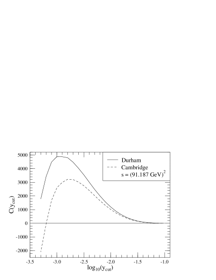
FIG. 2.: The correction function $C_{4}$ for the four-jet rate as a function of the resolution variable $y_{\rm cut}$ with Durham (solid) and Cambridge (dashed) algorithms.

TABLE I.: Correction functions to the four-jet rates for Durham and Cambridge algorithms.

$\log_{10}(y_{cut})$	$C_{y_{cut}}^{\rm D}$	$C_{y_{cut}}^{\rm C}$
$-0.9$	$\!\!(4.209\pm 0.655)\cdot 10^{-2}\!\!$	$\!\!(4.375\pm 0.655)\cdot 10^{-2}\!\!$
$-1.0$	$\!\!(9.449\pm 0.220)\cdot 10^{-1}\!\!$	$\!\!(9.499\pm 0.230)\cdot 10^{-1}\!\!$
$-1.1$	$\!\!(5.411\pm 0.055)\cdot 10^{0}\!\!$	$\!\!(5.300\pm 0.057)\cdot 10^{0}\!\!$
$-1.2$	$\!\!(1.769\pm 0.011)\cdot 10^{1}\!\!$	$\!\!(1.700\pm 0.012)\cdot 10^{1}\!\!$
$-1.3$	$\!\!(4.321\pm 0.032)\cdot 10^{1}\!\!$	$\!\!(4.044\pm 0.033)\cdot 10^{1}\!\!$
$-1.4$	$\!\!(8.893\pm 0.034)\cdot 10^{1}\!\!$	$\!\!(8.142\pm 0.038)\cdot 10^{1}\!\!$
$-1.5$	$\!\!(1.619\pm 0.005)\cdot 10^{2}\!\!$	$\!\!(1.459\pm 0.006)\cdot 10^{2}\!\!$
$-1.6$	$\!\!(2.705\pm 0.009)\cdot 10^{2}\!\!$	$\!\!(2.400\pm 0.010)\cdot 10^{2}\!\!$
$-1.7$	$\!\!(4.201\pm 0.012)\cdot 10^{2}\!\!$	$\!\!(3.683\pm 0.014)\cdot 10^{2}\!\!$
$-1.8$	$\!\!(6.221\pm 0.020)\cdot 10^{2}\!\!$	$\!\!(5.403\pm 0.021)\cdot 10^{2}\!\!$
$-1.9$	$\!\!(8.730\pm 0.029)\cdot 10^{2}\!\!$	$\!\!(7.490\pm 0.032)\cdot 10^{2}\!\!$
$-2.0$	$\!\!(1.191\pm 0.004)\cdot 10^{3}\!\!$	$\!\!(1.009\pm 0.005)\cdot 10^{3}\!\!$
$-2.1$	$\!\!(1.563\pm 0.006)\cdot 10^{3}\!\!$	$\!\!(1.308\pm 0.007)\cdot 10^{3}\!\!$
$-2.2$	$\!\!(2.000\pm 0.010)\cdot 10^{3}\!\!$	$\!\!(1.653\pm 0.010)\cdot 10^{3}\!\!$
$-2.3$	$\!\!(2.478\pm 0.011)\cdot 10^{3}\!\!$	$\!\!(2.023\pm 0.012)\cdot 10^{3}\!\!$
$-2.4$	$\!\!(3.007\pm 0.024)\cdot 10^{3}\!\!$	$\!\!(2.402\pm 0.025)\cdot 10^{3}\!\!$
$-2.5$	$\!\!(3.542\pm 0.023)\cdot 10^{3}\!\!$	$\!\!(2.749\pm 0.027)\cdot 10^{3}\!\!$
$-2.6$	$\!\!(4.029\pm 0.033)\cdot 10^{3}\!\!$	$\!\!(3.020\pm 0.036)\cdot 10^{3}\!\!$
$-2.7$	$\!\!(4.469\pm 0.052)\cdot 10^{3}\!\!$	$\!\!(3.198\pm 0.063)\cdot 10^{3}\!\!$
$-2.8$	$\!\!(4.797\pm 0.067)\cdot 10^{3}\!\!$	$\!\!(3.220\pm 0.077)\cdot 10^{3}\!\!$
$-2.9$	$\!\!(4.869\pm 0.099)\cdot 10^{3}\!\!$	$\!\!(2.999\pm 0.108)\cdot 10^{3}\!\!$
$-3.0$	$\!\!(4.878\pm 0.120)\cdot 10^{3}\!\!$	$\!\!(2.608\pm 0.132)\cdot 10^{3}\!\!$
$-3.1$	$\!\!(4.482\pm 0.166)\cdot 10^{3}\!\!$	$\!\!(1.678\pm 0.178)\cdot 10^{3}\!\!$
$-3.2$	$\!\!(3.430\pm 0.256)\cdot 10^{3}\!\!$	$\!\!(-3.254\pm 27.6)\cdot 10^{1}\!\!$
$-3.3$	$\!\!(1.783\pm 0.300)\cdot 10^{3}\!\!$	$\!\!(-2.093\pm 0.32)\cdot 10^{3}\!\!$

Comparing the values for the two Born functions, we see that at leading order the Cambridge algorithm gives slightly higher rates and the difference increases with decreasing $y_{\rm cut}$. On the other hand, the correction functions become smaller for Cambridge clustering with decreasing $y_{\rm cut}$. The result of these opposite trends is that the $K$ factors, defined as

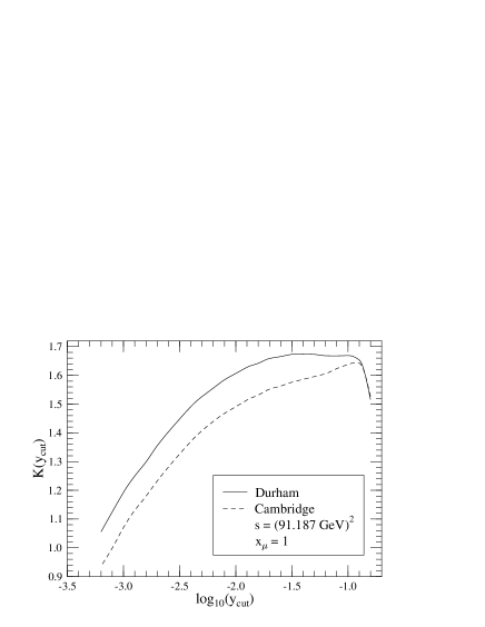
FIG. 3.: $K$ factors as a function of the resolution variable $y_{\rm cut}$ for Durham (solid) and Cambridge (dashed) algorithms.

$$K(y_{\rm cut})=1+\eta(\sqrt{s})\frac{C_{4}(y_{\rm cut})}{B_{4}(y_{\rm cut})}\>,$$ (55)

are smaller for the Cambridge algorithm for small values of $y_{\rm cut}$, which is demonstrated in Fig. 3.

The smaller $K$ factors also mean smaller renormalization scheme dependence, which can be seen from comparing Figs. 4 and 5. The usual interpretation of the smaller scale dependence is that the effect of the uncalculated higher orders are expected to be smaller in the case of Cambridge clustering. It is interesting to note that in the middle $y_{\rm cut}$ region ($10^{-3.2}<y_{\rm cut}<10^{-2}$), where the hadronization corrections for the Cambridge clustering were found significantly larger than for the Durham algorithm, the theoretical uncertainty due to the renormalization scale ambiguity is smaller for the Cambridge than that for the Durham clustering. Of course, one has to keep in mind that the $\mu$-dependence bands are not upper bounds on errors that arise from truncation of the perturbation series, just suggestions. In particular, if there is an artificial narrowing of the $\mu$-dependence bands, e.g. at a crossover point, they almost certainly do not represent the size of the truncation error at that point.

Four-jet fractions decrease very rapidly with increasing resolution parameter $y_{\rm cut}$. As a result, most of the available four-jet data are below $y_{\rm cut}=0.01$. It is well-known that for small values of $y_{\rm cut}$ the fixed order perturbative prediction is not reliable, because the expansion parameter ${\alpha_{s}}\ln^{2}y_{\rm cut}$ logarithmically enhances the higher order corrections. One has to perform the all order resummation of the leading and next-to-leading logarithmic (NLL) contributions. This resummation is possible for the Durham algorithm using the coherent branching formalism [29] and the procedure is the same for the Cambridge algorithm [23]. The four-jet rate in the next-to-leading logarithmic approximation is given by [29]

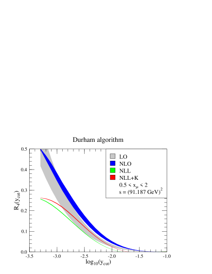
FIG. 4.: The QCD prediction for the four-jet rate with Durham clustering at Born level (light gray band) and at next-to-leading order (dark band). The two narrow bands show the four-jet rate in the NLL approximation ($K=0$, lower band) and in improved NLL approximation (upper band) as explained in the text. The bands indicate the theoretical uncertainty due to the variation of the renormalization scale $x_{\mu}$ between 0.5 and 2.

$$R_{4}^{\rm NLL}=2[\Delta_{q}(Q)]^{2}\Bigg{[}\left(\int_{Q_{0}}^{Q}\!{\rm d}q\,\Gamma_{q}(Q,q)\,\Delta_{g}(q,Q_{0})\right)^{2}$$ (56)

$$\quad+\int_{Q_{0}}^{Q}\!{\rm d}q\,\Gamma_{q}(Q,q)\,\Delta_{g}(q,Q_{0})$$ (57)

$$\quad\times\int_{Q_{0}}^{q}\!{\rm d}q^{\prime}\,\Big{(}\Gamma_{g}(q,q^{\prime})\,\Delta_{g}(q^{\prime},Q_{0})+\Gamma_{f}(q^{\prime})\Delta_{f}(q^{\prime},Q_{0})\Big{)}\Bigg{]}\>.$$ (58)

In Eq. (56) the functions $\Delta_{a}(Q,Q_{0})$ are the Sudakov form factors which express the probability of parton branching evolution from scale $Q_{0}=Q\sqrt{y_{\rm cut}}$ to scale $Q$ without resolvable branching. The Sudakov factors are defined in terms of the $P_{ab}({\alpha_{s}}(q),z)$ vertex probabilities as follows

$$\Delta_{a}(Q,Q_{0})=$$ (59)

$$\quad\exp\left(-\sum_{b}\int_{Q_{0}}^{Q}\!\frac{{\rm d}q}{q}\int\!{\rm d}z\,\frac{{\alpha_{s}}(q)}{2\pi}\,P_{ab}({\alpha_{s}}(q),z)\right)\>.$$ (60)

It was shown in Ref. [30] that one can obtain an improved theoretical prediction for the differential two-jet rate if the vertex probabilities are taken at next-to-leading order [31], which we also consider in our analysis:

$$P_{qq}({\alpha_{s}},z)=C_{F}\left(\frac{1+z^{2}}{1-z}+\frac{{\alpha_{s}}}{2\pi}\,K\,\frac{2}{1-z}\right)\>,$$ (61)

$$P_{gg}({\alpha_{s}},z)=$$ (62)

$$\quad 2C_{A}\left(\frac{z}{1-z}+\frac{1-z}{z}+z(1-z)+\frac{{\alpha_{s}}}{2\pi}\,K\,\frac{2}{z(1-z)}\right)\>,$$ (63)

$$P_{gq}({\alpha_{s}},z)=T_{R}{N_{\rm f}}\left(z^{2}+(1-z)^{2}\right)\>.$$ (64)

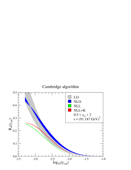
FIG. 5.: The QCD prediction for the four-jet rate with Cambridge clustering at Born level (light gray band) and at next-to-leading order (dark band). The two narrow bands show the four-jet rate in the NLL approximation ($K=0$, lower band) and in improved NLL approximation (upper band) as explained in the text. The bands indicate the theoretical uncertainty due to the variation of the renormalization scale $x_{\mu}$ between 0.5 and 2.

The $K$ coefficient is renormalization scheme dependent. In the $\overline{{\rm MS}}$ scheme it is given by [32]

$$K=C_{A}\left(\frac{67}{18}-\frac{\pi^{2}}{6}\right)-\frac{10}{9}T_{R}{N_{\rm f}}\>.$$ (65)

Performing the $z$ integral in Eq. (59), one obtains the Sudakov factors as integrals of the emission probabilities $\Gamma_{a}(Q,q)$ in the following form:

$$\Delta_{q}(Q,Q_{0})=\exp\left(-\int_{Q_{0}}^{Q}\!{\rm d}q\,\Gamma_{q}(Q,q)\right)\>,$$ (66)

$$\Delta_{g}(Q,Q_{0})=$$ (67)

$$\qquad\exp\left(-\int_{Q_{0}}^{Q}\!{\rm d}q\,\left[\Gamma_{g}(Q,q)+\Gamma_{f}(q)\right]\right)\>,$$ (68)

$$\Delta_{f}(Q,Q_{0})=\frac{\left[\Delta_{q}(Q,Q_{0})\right]^{2}}{\Delta_{g}(Q,Q_{0})}\>,$$ (69)

and the NLL emission probabilities are

$$\Gamma_{q}(Q,q)=$$ (70)

$$\qquad\frac{2C_{F}}{\pi}\frac{{\alpha_{s}}(q)}{q}\left[\left(1+\frac{{\alpha_{s}}(q)}{2\pi}\,K\right)\ln\frac{Q}{q}-\frac{3}{4}\right]\>,$$ (71)

$$\Gamma_{g}(Q,q)=$$ (72)

$$\qquad\frac{2C_{A}}{\pi}\frac{{\alpha_{s}}(q)}{q}\left[\left(1+\frac{{\alpha_{s}}(q)}{2\pi}\,K\right)\ln\frac{Q}{q}-\frac{11}{12}\right]\>,$$ (73)

$$\Gamma_{f}(Q,q)=\frac{{N_{\rm f}}}{3\pi}\frac{{\alpha_{s}}(q)}{q}\>.$$ (74)

We relate the ${\alpha_{s}}(q)$ strong coupling appearing in the emission probabilities to the strong coupling at the relevant renormalization scale, ${\alpha_{s}}(\mu)$, according to the one-loop formula

$${\alpha_{s}}(q)=\frac{{\alpha_{s}}(\mu)}{w(q,\mu)}\>,$$ (75)

where $w(q,q_{0})$ was defined in Eq. (45), and we use Eq. (44) for expressing ${\alpha_{s}}(\mu)$ in terms of ${\alpha_{s}}(M_{Z})=0.118$. We could also use a two-loop formula for ${\alpha_{s}}(q)$, but the result would differ only in subleading logarithms.

The result of this resummation together with its renormalization scale dependence is also shown in Figs. 4 and 5 (narrow bands). The lower band corresponds to the usual NLL approximation ($K=0$), and the upper band is the result of the improved resummation. We can see clearly from the figures that the fixed-order and the NLL approximations differ significantly. One expects that for large values of $y_{\rm cut}$ the former, and for small values of $y_{\rm cut}$ the latter is the reliable description, therefore, the two results have to matched.

The Durham and Cambridge four-jet rates can be resummed at leading and next-to-leading logarithmic order, but they do not satisfy a simple exponentiation [33]. For observables that do not exponentiate the viable matching schemes are the R matching or the modified R matching [29, 4]. We use R matching according to the following formula:

$$R_{4}^{\rm R-match}=R_{4}^{\rm NLL}+\Bigg{[}\eta^{2}\left(B_{4}-B_{4}^{\rm NLL}\right)$$ (76)

$$\qquad\qquad\qquad+\eta^{3}\left(C_{4}-C_{4}^{\rm NLL}-\frac{3}{2}\left(B_{4}-B_{4}^{\rm NLL}\right)\right)\Bigg{]}\>,$$ (77)

where $B_{4}^{\rm NLL}$ and $C_{4}^{\rm NLL}$ are the coefficients in the expansion of $R_{4}^{\rm NLL}$ as in Eq. (53).

In Fig. 6 we show the theoretical prediction at the various levels of approximation: in fixed order perturbation theory at Born level (LO), at next-to-leading order (NLO), resummed and R-matched prediction (NLO+NLL) and improved resummed and R-matched prediction (NLO+NLL+K). Also shown is the four-jet rate measured by the ALEPH collaboration at the $Z^{0}$ peak [34] corrected to parton level using the PYTHIA Monte Carlo [35]. We used bin-by-bin correction and the consistency of the correction was checked by using the HERWIG Monte Carlo [36]. The two programs gave the same correction factor within statistical error. The errors of the data are the scaled errors of the published hadron level data, and we did not include any systematic error due to the hadron to parton correction. In the inset we indicated the renormalization scale dependence of the ‘NLO+NLL+K’ prediction.

FIG. 6.: The QCD prediction for the four-jet rate with Durham clustering in fixed order perturbation theory at leading (dotted) and next-to-leading order (dashed), and fixed order matched with resummed (dashed-dotted) and improved resummed (solid) calculation compared to ALEPH data obtained at the $Z^{0}$ peak and corrected to parton level (errorbars). The renormalization scale is set to $x_{\mu}=1$. The lower plot shows the relative difference $\delta_{4}=$ (data–theory)/theory, where theory means the next-to-leading order prediction matched with improved resummed calculation at $x_{\mu}=1$. The inset shows the renormalization scale dependence of the ‘theory’ prediction with scale variation $0.5<x_{\mu}<2$.

Fig. 6 deserves several remarks. First of all, we see that the inclusion of the radiative corrections improves the fixed order description of the data using the natural scale $x_{\mu}=1$ for larger values of $y_{\rm cut}$. Secondly, the importance of resummation in the small $y_{\rm cut}$ region is clearly seen, but it is still not sufficient to describe the data at the natural scale, neglected subleading terms are still important. On the other hand, the improved resummation seems to take into account just the right amount of subleading terms and it makes the agreement between data and theory almost perfect over the whole $y_{\rm cut}$ region as can be seen from the lower plot. (Although for $y_{\rm cut}>10^{-1.7}$ $\delta_{4}$ falls outside the $\pm 5\,\%$ band, one should keep in mind that in this region the error of the hadron to parton correction is very large. Also, for the ‘NLO+NLL+K’ prediction we found remarkably small scale dependence for $y_{\rm cut}>10^{-3}$. This feature, however, should be taken with care. The improvement, obtained by including the two-loop coefficient K, affects NNLL terms, but there are other contributions of the same order that are not taken into account (e.g., next-to-leading order running of ${\alpha_{s}}$ and other dynamical effects), which is not the case for the 2-jet rate. The scale dependence of the ‘NLO+NLL+K’ result would consistently be under control only after the inclusion of the complete set of NNLL terms.

Finally it is worth noting that for $y_{\rm cut}=10^{-2.6}$ both PYTHIA and HERWIG yield less than 2 % hadronization correction. At the same value of the resolution parameter the theoretical prediction is insensitive to corrections beyond next-to-leading order (the NLO, NLO+NLL, NLO+NLL+K curves cross, the renormalization scale dependence is small), therefore, at this accidental value of $y_{\rm cut}$ the next-to-leading order prediction agrees perfectly with the hadron level data.

B Four-jet event shapes

Four-jet event shapes were used extensively by the LEP collaborations for QCD studies [34, 37]. In this subsection we consider four shape variables, the $y_{4}$ distributions for the Durham and Cambridge algorithms, the thrust minor ($T_{\rm min}$) and the C parameter for C values above 0.75, which are often used in the experimental analyses.

In the case of event shape distributions we multiply the normalized cross section with the value of the event shape parameter, so we use the parametrisation

$$\Sigma(O_{4})\equiv O_{4}\frac{1}{\sigma_{0}}\frac{{\rm d}\sigma}{{\rm d}O_{4}}(O_{4})$$ (78)

$$\qquad=\eta(\mu)^{2}B(O_{4})+\eta(\mu)^{3}\left[B(O_{4})\frac{\beta_{0}}{C_{F}}\ln x_{\mu}^{2}+C(O_{4})\right]$$ (79)

instead of Eq. (42), in which case the average value of the shape variable is easily obtained from the differential distribution:

$$<O_{4}>_{\delta}=\int_{\delta}^{1}\!{\rm d}O_{4}\,\Sigma(O_{4})\>.$$ (80)

Using this parametrisation we define the $K$ factors of the differential distribution as

$$K(O_{4})=1+\eta(\sqrt{s})\,\frac{C(O_{4})}{B(O_{4})}\>.$$ (81)

In the following we plot the physical cross sections $\Sigma(O_{4})$, the $K(O_{4})$ factors and tabulate the correction functions $C(O_{4})$ for $O_{4}=y_{4}$, $T_{\rm min}$ and C.

The $y_{4}$ value denotes the transition value for $y_{\rm cut}$ at which, when decreasing $y_{\rm cut}$, the classification of a given event changes from three jets to four jets. The advantage of this variable over the differential four-jet rate is that this variable can be defined on an event by event basis. Depending on the actual resolution variable one obtains the $y_{4}^{D}$ distribution for the Durham clustering and the $y_{4}^{C}$ distribution for the Cambridge clustering. We calculated the $B(y_{4})$ and $C(y_{4})$ functions for both algorithms. The $B(y_{4})$ values equal the $y_{\rm cut}B(y_{\rm cut})$ values when $y_{4}=y_{\rm cut}$, therefore, we tabulate only the $C(y_{4})$ functions for the two algorithms in Table II.

TABLE II.: Correction functions to the differential distributions of the $y_{4}$ variables for the Durham and Cambridge algorithm. The parameter values are at the lower edge of the corresponding histogram bin.

$y_{4}$	$C_{y_{4}}^{\rm D}$	$C_{y_{4}}^{\rm C}$
0.000	$\!\!(2.523\pm 0.425)\cdot 10^{3}\!\!$	$\!\!(1.064\pm 0.350)\cdot 10^{3}\!\!$
0.005	$\!\!(2.212\pm 0.017)\cdot 10^{3}\!\!$	$\!\!(1.857\pm 0.019)\cdot 10^{3}\!\!$
0.010	$\!\!(1.376\pm 0.009)\cdot 10^{3}\!\!$	$\!\!(1.166\pm 0.011)\cdot 10^{3}\!\!$
0.015	$\!\!(9.429\pm 0.071)\cdot 10^{2}\!\!$	$\!\!(8.144\pm 0.080)\cdot 10^{2}\!\!$
0.020	$\!\!(6.799\pm 0.070)\cdot 10^{2}\!\!$	$\!\!(5.855\pm 0.062)\cdot 10^{2}\!\!$
0.025	$\!\!(4.930\pm 0.063)\cdot 10^{2}\!\!$	$\!\!(4.346\pm 0.051)\cdot 10^{2}\!\!$
0.030	$\!\!(3.760\pm 0.042)\cdot 10^{2}\!\!$	$\!\!(3.293\pm 0.043)\cdot 10^{2}\!\!$
0.035	$\!\!(2.885\pm 0.037)\cdot 10^{2}\!\!$	$\!\!(2.553\pm 0.039)\cdot 10^{2}\!\!$
0.040	$\!\!(2.164\pm 0.033)\cdot 10^{2}\!\!$	$\!\!(1.947\pm 0.034)\cdot 10^{2}\!\!$
0.045	$\!\!(1.754\pm 0.026)\cdot 10^{2}\!\!$	$\!\!(1.580\pm 0.027)\cdot 10^{2}\!\!$
0.050	$\!\!(1.314\pm 0.025)\cdot 10^{2}\!\!$	$\!\!(1.202\pm 0.025)\cdot 10^{2}\!\!$
0.055	$\!\!(1.024\pm 0.021)\cdot 10^{2}\!\!$	$\!\!(9.508\pm 0.213)\cdot 10^{1}\!\!$
0.060	$\!\!(8.293\pm 0.292)\cdot 10^{1}\!\!$	$\!\!(7.692\pm 0.296)\cdot 10^{1}\!\!$
0.065	$\!\!(6.307\pm 0.300)\cdot 10^{1}\!\!$	$\!\!(5.945\pm 0.304)\cdot 10^{1}\!\!$
0.070	$\!\!(4.636\pm 0.180)\cdot 10^{1}\!\!$	$\!\!(4.445\pm 0.184)\cdot 10^{1}\!\!$
0.075	$\!\!(3.516\pm 0.117)\cdot 10^{1}\!\!$	$\!\!(3.430\pm 0.114)\cdot 10^{1}\!\!$
0.080	$\!\!(2.673\pm 0.115)\cdot 10^{1}\!\!$	$\!\!(2.560\pm 0.110)\cdot 10^{1}\!\!$
0.085	$\!\!(2.271\pm 0.216)\cdot 10^{1}\!\!$	$\!\!(2.214\pm 0.217)\cdot 10^{1}\!\!$
0.090	$\!\!(1.412\pm 0.204)\cdot 10^{1}\!\!$	$\!\!(1.395\pm 0.206)\cdot 10^{1}\!\!$
0.095	$\!\!(1.085\pm 0.057)\cdot 10^{1}\!\!$	$\!\!(1.056\pm 0.059)\cdot 10^{1}\!\!$
0.100	$\!\!(7.412\pm 0.584)\cdot 10^{0}\!\!$	$\!\!(7.377\pm 0.588)\cdot 10^{0}\!\!$
0.105	$\!\!(5.069\pm 0.537)\cdot 10^{0}\!\!$	$\!\!(5.121\pm 0.529)\cdot 10^{0}\!\!$
0.110	$\!\!(2.817\pm 0.400)\cdot 10^{0}\!\!$	$\!\!(2.914\pm 0.399)\cdot 10^{0}\!\!$
0.115	$\!\!(2.652\pm 0.329)\cdot 10^{0}\!\!$	$\!\!(2.428\pm 0.301)\cdot 10^{0}\!\!$
0.120	$\!\!(1.353\pm 0.221)\cdot 10^{0}\!\!$	$\!\!(1.516\pm 0.183)\cdot 10^{0}\!\!$

We show the next-to-leading order perturbative prediction in QCD for $\Sigma(y_{4})$ in Fig. 7. In the same figure, the inset shows the $K(y_{4})$ factors of the distributions. The physical cross sections for the two algorithms are very similar. The $K(y_{4})$ factors are quite large, but much smaller than in the case of other four-jet event shape distributions. They depend weakly on the $y_{4}$ value for $y_{4}>0.1$ and decrease rapidly with decreasing $y_{4}$ below $y_{4}=0.1$. In the case of the Cambridge algorithm the radiative corrections are 15–30 % smaller than those for the Durham algorithm.

In order to define $T_{\rm min}$, we first have to define the thrust and thrust major axes [38]. The thrust axis $\vec{n}_{T}$ is the direction $\vec{n}$ which maximizes the expression

$$T=\max_{\vec{n}_{T}}\left(\frac{\sum_{a}|\vec{p}_{a}\cdot\vec{n}|}{\sum_{a}|\vec{p}_{a}|}\right),$$ (82)

FIG. 7.: The next-to-leading order QCD prediction for the $y_{4}^{D}$ (solid) and $y_{4}^{C}$ (dashed) differential distributions with renormalization scale $x_{\mu}=1$. The inset shows the $K$ factors of the distributions.

where the sum runs over all final state hadrons (or partons). The thrust major axis is a three-vector $\vec{n}_{T_{\rm maj}}$ for which the expression in Eq. (82) is maximal with the constraint that $\vec{n}_{T_{\rm maj}}$ is perpendicular to $\vec{n}_{T}$, $\vec{n}_{T_{\rm maj}}\cdot\vec{n}_{T}=0$. In order to obtain the value of $T_{\rm min}$, one evaluates the expression in the parentheses for a vector perpendicular to both $\vec{n}_{T_{\rm maj}}$ and $\vec{n}_{T}$.

The C parameter [39] is derived from the eigenvalues of the infrared safe momentum tensor

$$\theta^{ij}=\sum_{a}\frac{p_{a}^{i}p_{a}^{j}}{|\vec{p}_{a}|}\bigg{/}\sum_{a}|\vec{p}_{a}|,$$ (83)

where the sum on $a$ runs over all final state hadrons and $p_{a}^{i}$ is the $i$th component of the three-momentum $\vec{p}_{a}$ of hadron $a$ in the c.m. system. The tensor $\theta$ is normalized to have unit trace. In terms of the eigenvalues $\lambda_{i}$ of the $3\times 3$ matrix $\theta$, the global shape parameter C is defined as

$${\rm C}=3\,(\lambda_{1}\lambda_{2}+\lambda_{2}\lambda_{3}+\lambda_{3}\lambda_{1})\>.$$ (84)

The kinematical limit of the C parameter for three-parton processes is C = 0.75. Therefore, in the region C $\in[0.75,1]$ the four-parton processes contribute to the leading order prediction, and our program is capable to calculate the radiative correction to the distribution. The results of such a calculation for the Born functions $B_{T_{\rm min}}$ and $B_{\rm C}$ agree with the known results (see e.g., [40]) The $C_{T_{\rm min}}$ and $C_{\rm C}$ correction functions are given in Table III.

TABLE III.: Correction functions to the differential distributions of the $T_{\rm min}$ and C parameter event shape variables. The parameter values are at the lower edge of the corresponding histogram bin.

$T_{\rm min}$	$C_{T_{\rm min}}$	${\rm C}$	$C_{\rm C}$
0.00	–	0.75	$\!\!(4.775\pm 1.100)\cdot 10^{3}\!\!$
0.02	$\!\!(3.319\pm 0.270)\cdot 10^{4}\!\!$	0.76	$\!\!(6.082\pm 0.160)\cdot 10^{3}\!\!$
0.04	$\!\!(2.381\pm 0.082)\cdot 10^{4}\!\!$	0.77	$\!\!(4.610\pm 0.089)\cdot 10^{3}\!\!$
0.06	$\!\!(1.652\pm 0.038)\cdot 10^{4}\!\!$	0.78	$\!\!(3.663\pm 0.063)\cdot 10^{3}\!\!$
0.08	$\!\!(1.172\pm 0.025)\cdot 10^{4}\!\!$	0.79	$\!\!(2.904\pm 0.042)\cdot 10^{3}\!\!$
0.10	$\!\!(8.600\pm 0.130)\cdot 10^{3}\!\!$	0.80	$\!\!(2.406\pm 0.031)\cdot 10^{3}\!\!$
0.12	$\!\!(6.488\pm 0.100)\cdot 10^{3}\!\!$	0.81	$\!\!(1.948\pm 0.026)\cdot 10^{3}\!\!$
0.14	$\!\!(4.695\pm 0.077)\cdot 10^{3}\!\!$	0.82	$\!\!(1.625\pm 0.024)\cdot 10^{3}\!\!$
0.16	$\!\!(3.499\pm 0.042)\cdot 10^{3}\!\!$	0.83	$\!\!(1.365\pm 0.023)\cdot 10^{3}\!\!$
0.18	$\!\!(2.684\pm 0.027)\cdot 10^{3}\!\!$	0.84	$\!\!(1.135\pm 0.019)\cdot 10^{3}\!\!$
0.20	$\!\!(2.010\pm 0.021)\cdot 10^{3}\!\!$	0.85	$\!\!(9.194\pm 0.130)\cdot 10^{2}\!\!$
0.22	$\!\!(1.498\pm 0.017)\cdot 10^{3}\!\!$	0.86	$\!\!(7.906\pm 0.110)\cdot 10^{2}\!\!$
0.24	$\!\!(1.122\pm 0.013)\cdot 10^{3}\!\!$	0.87	$\!\!(6.293\pm 0.092)\cdot 10^{2}\!\!$
0.26	$\!\!(8.247\pm 0.100)\cdot 10^{2}\!\!$	0.88	$\!\!(5.217\pm 0.084)\cdot 10^{2}\!\!$
0.28	$\!\!(6.093\pm 0.074)\cdot 10^{2}\!\!$	0.89	$\!\!(4.296\pm 0.066)\cdot 10^{2}\!\!$
0.30	$\!\!(4.501\pm 0.180)\cdot 10^{2}\!\!$	0.90	$\!\!(3.391\pm 0.052)\cdot 10^{2}\!\!$
0.32	$\!\!(3.026\pm 0.057)\cdot 10^{2}\!\!$	0.91	$\!\!(2.815\pm 0.061)\cdot 10^{2}\!\!$
0.34	$\!\!(2.229\pm 0.050)\cdot 10^{2}\!\!$	0.92	$\!\!(2.075\pm 0.057)\cdot 10^{2}\!\!$
0.36	$\!\!(1.549\pm 0.046)\cdot 10^{2}\!\!$	0.93	$\!\!(1.626\pm 0.032)\cdot 10^{2}\!\!$
0.38	$\!\!(1.095\pm 0.028)\cdot 10^{2}\!\!$	0.94	$\!\!(1.221\pm 0.026)\cdot 10^{2}\!\!$
0.40	$\!\!(7.100\pm 0.210)\cdot 10^{1}\!\!$	0.95	$\!\!(8.154\pm 0.260)\cdot 10^{1}\!\!$
0.42	$\!\!(4.437\pm 0.180)\cdot 10^{1}\!\!$	0.96	$\!\!(5.193\pm 0.190)\cdot 10^{1}\!\!$
0.44	$\!\!(2.684\pm 0.190)\cdot 10^{1}\!\!$	0.97	$\!\!(3.165\pm 0.130)\cdot 10^{1}\!\!$
0.46	$\!\!(1.439\pm 0.150)\cdot 10^{1}\!\!$	0.98	$\!\!(1.312\pm 0.094)\cdot 10^{1}\!\!$
0.48	$\!\!(6.447\pm 0.560)\cdot 10^{0}\!\!$	0.99	$\!\!(2.769\pm 0.260)\cdot 10^{0}\!\!$

In the case of event shape differential distributions the next-to-leading order corrections should logarithmically diverge at the edge of the phase space. This divergence occurs at zero for the $y_{4}$ and $T_{\rm min}$ distributions and is regularized by the multiplication with the value of the variable (see Eq. (78)). This is not the case for the C parameter, because it diverges at C = 0.75. Nevertheless, we obtained a finite and positive contribution in the first bin owing to bin smearing as we have checked explicitly by refining the bin width.

Figs. 8 and 9 show the leading and next-to-leading order QCD prediction for the $T_{\rm min}$ and C parameter differential distributions at $x_{\mu}=1$. The insets show the $K$ factors which are large in both cases indicating 100 % or larger radiative corrections. As a result, the renormalization scale dependence remains large, only the absolute normalization of the distributions increases with a factor of more than 2 with the inclusion of the radiative corrections. This feature is demonstrated in Fig. 10, where we show the scale dependence of the leading and next-to-leading order prediction for the average value of the thrust minor (above $T_{\rm min}=0.02$) and C parameter (above C = 0.75). The leading and next-to-leading order curves run almost parallel down to $x_{\mu}\simeq 0.2$, only the latter is shifted to larger values.

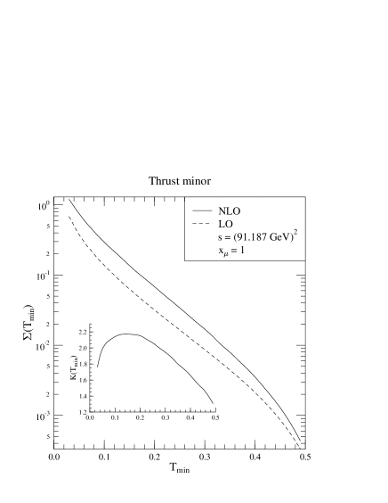
FIG. 8.: The leading-order (dashed) and the next-to-leading order (solid) QCD prediction for the $T_{\rm min}$ variable with renormalization scale $x_{\mu}=1$. The inset shows the $K$ factor of the distribution.

FIG. 9.: The leading-order (dashed) and the next-to-leading order (solid) QCD prediction for the C parameter with renormalization scale $x_{\mu}=1$. The inset shows the $K$ factor of the distribution.

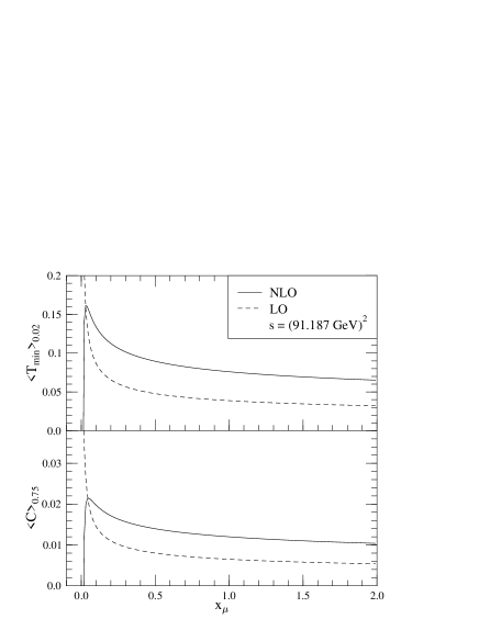
FIG. 10.: The renormalization scale dependence of the average values of $<T_{\rm min}>_{0.02}$ and $<{\rm C}>_{0.75}$ at leading and next-to-leading order.

C Radiative corrections to four-jet observables: summary

In this subsection we summarize the results of our radiative correction calculations for the various four-jet like distributions presented in previous publications and in this article.

The QCD prediction at tree level (with renormalization scale $x_{\mu}=1$) is in general falls significantly below the measured values for unnormalised distributions of four-jet observables. Consequently, the calculation of the next-to-leading order corrections to these cross sections is indispensable for attempting a serious comparison between data and theory. Our calculations show that the corrections are very large and the agreement in the comparison improves considerably with the inclusion of the radiative corrections. In particular, we found the following features:
(1) In the case of four-jet rates, the radiative corrections are about 100 % for JADE-type clustering algorithms [11, 13], while for the Durham algorithm it is less than 60 % and even smaller for the Cambridge algorithm. The scale dependence for the latter algorithms is substantially reduced. The agreement between data and theory for the Durham clustering is very good and extends to small values of $y_{\rm cut}$ when one matches the fixed order prediction with improved resummed next-to-leading logarithmic approximation.
(2) In the case of event shape variables the corrections are usually more than 100 % (the $K$ factors are larger than 2). The residual renormalization scale dependence is large indicating that even higher orders are important. One may conclude that, with the exception of the jet-related $y_{4}$ distributions, these distributions cannot be reliably calculated in fixed order perturbation theory and cannot be used for precision tests of QCD.
(3) In the case of normalized angular distributions the corrections are small as expected (the $K$ factors are close to 1) [12, 15]. The renormalization scale dependence is small, which however, does not mean that the effect of the radiative corrections on the measurement of the QCD color charges is negligible. According to Ref. [15], the measured value of the $T_{R}/C_{F}$ ratio may differ up to 25 % when leading, or next-to-leading order QCD predictions are used in the color charge fits.

IV Conclusions

This paper dealt with the next-to-leading order calculation of four-jet observables in electron-positron annihilation. We gave details of the analytical calculation that lead to the construction of a Monte Carlo program [41] which can be used to calculate the differential distribution of any four-jet observable at the O($\alpha_{s}^{3}$) accuracy. The dipole method was used for achieving the analytical cancellation of infrared divergences. We described that modification of the algorithm which we found useful from numerical point of view. However, the modification is not essential as far as the theory is concerned.

Compact formulas were presented for the Born-level five-parton helicity amplitudes and for the Born-level four-parton color-correlated matrix elements which are necessary for other next-to-leading order calculations, such as the next-to-leading order cross section of three-jet production in deep inelastic scattering and that of vector boson plus two-jet production in hadron collisions. We also gave a group independent decomposition of the Born-level five-parton matrix elements.

We calculated the next-to-leading order corrections to the four-jet rates with the Durham and Cambridge jet clustering algorithms and to the differential distributions of the $y_{4}$, thrust minor and C parameter (at C $\geq$ 0.75) four-jet shape variables. In the case of four-jet rates the radiative corrections were found to be large, but just acceptable. The renormalization scale dependence decreased significantly and the fixed order result matched with the next-to-leading logarithmic approximation gave remarkably good agreement with LEP data over a wide range of the resolution variable. The high level of agreement implies that the QCD four-jet background to $W^{\pm}$ pair production at higher center of mass energies can be predicted in perturbation theory reliably. In the case of event shape variables the radiative corrections and the renormalization scale dependence are unacceptably large suggesting that the next-to-leading order prediction is not reliable and even higher orders are important.

A Helicity amplitudes

In this appendix we present analytic formulas for the four- and five-parton tree-level helicity amplitudes of the relevant subprocesses. These amplitudes were first calculated in Refs. [21]. The reason for presenting our results here is twofold. On one hand we express the relevant color subamplitudes in terms of Weyl spinors $|{k\pm}\rangle$, which were also employed in the case of the one-loop four-parton amplitudes [20], while on the other we found that our expressions in the case of the four-quark processes are more compact and the corresponding computer code is faster than earlier ones. Another new feature of the amplitudes in this appendix is that we allow for the existence of light fermionic degrees of freedom in the adjoint representation of the gauge group (light gluinos). In calculating the amplitudes, we used quark and gluon currents [42, 44] and standard helicity techniques [43, 44].

We consider three subprocesses, each involving a vector boson $V(Q)$ carrying total four-momentum $Q$ and $n$ QCD partons ($n=4$, or 5 here). The first subprocess is the production of a quark-antiquark pair and $n-2$ gluons. The second one is the production of two quark-antiquark pairs (of equal, or unequal flavor) and $n-4$ gluons. Finally, the third process is the production of a quark-antiquark pair, a light-gluino pair and $n-4$ gluons:

$$\ell^{+}(-p_{\ell})+\ell^{-}(-p_{\bar{\ell}})\to V(Q)\to$$ (A2)

$$\qquad q(p_{1})+g_{1}(p_{2})+\dots+g_{n-2}(p_{n-1})+\bar{q}(p_{n})\>,$$

(A6)

$$\ell^{+}(-p_{\ell})+\ell^{-}(-p_{\bar{\ell}})\to V(Q)\to$$

$$\qquad q(p_{1})+\bar{q}(p_{2})+Q(p_{3})+\bar{Q}(p_{4})$$

$$\qquad+g_{1}(p_{5})+\dots+g_{n-4}(p_{n})\>,$$

(A10)

$$\ell^{+}(-p_{\ell})+\ell^{-}(-p_{\bar{\ell}})\to V(Q)\to$$

$$\qquad q(p_{1})+\bar{q}(p_{2})+{\tilde{g}}(p_{3})+{\tilde{g}}(p_{4})$$

$$\qquad+g_{1}(p_{5})+\dots+g_{n-4}(p_{n})\>.$$

We have chosen the crossing invariant all particle outgoing kinematics with corresponding particle-antiparticle assignment, therefore, momentum conservation means

$$p_{\ell}+p_{\bar{\ell}}+p_{1}+p_{2}+p_{3}+p_{4}+p_{5}+\ldots+p_{n}=0\>.$$ (A11)

We shall express the amplitudes in terms of color subamplitudes. In the case of process (A2), the color basis is chosen to be product of generators in the fundamental representation (in this appendix we use the normalization $T_{R}=1$ in ${\rm Tr}(t^{a}t^{b})=T_{R}\,\delta^{ab}$ for the generators of the symmetry group), therefore, the helicity amplitudes have the decomposition:

$$|{1_{f}^{h_{1}},2_{g}^{h_{2}},\ldots,n_{\bar{f}}^{h_{n}}}\rangle_{n}=$$ (A12)

$$\qquad\sum_{\{2,\dots,n-1\}}\left(t^{a_{2}}\cdot\dots\cdot t^{a_{n-1}}\right)_{i_{1}{\bar{i}}_{n}}\,m(1_{f}^{h_{1}},\dots,n_{\bar{f}}^{h_{n}})\>,$$ (A13)

where $\{2,\dots,n-1\}$ denotes all permutations of the labels $(2,\dots,n-1)$ and $m(1,\dots,n)$ are the color subamplitudes. In Eq. (A12) and in the following formulas the lepton labels are suppressed.

In the case of the four-fermion subprocesses (processes (A6) and (A10)) we decompose the helicity amplitudes as follows:

$$|{1_{f_{1}}^{h_{1}},2_{f_{2}}^{h_{2}},3_{f_{3}}^{h_{3}},4_{f_{4}}^{h_{4}},5_{g}^{h_{5}},\dots,n_{g}^{h_{n}}}\rangle_{n}=$$ (A14)

$$\qquad\sum_{\{5,\dots,n\}}\sum_{\{1,3\}}(-1)^{P}\sum_{\{2,4\}}(-1)^{P}{\cal A}_{n}(1,2,3,4,5,\dots,n)\>.$$ (A15)

where $P=0$ if the elements are in the canonical order ((1,3), or (2,4)) and $P=1$ if the elements are permuted ((3,1), or (4,2)). The partial amplitudes ${\cal A}_{n}$ can be decomposed further in color space. In the case of four-quark production,

$${\cal A}_{4}(1_{q},2_{\bar{q}},3_{Q},4_{\bar{Q}})=$$ (A16)

$$\qquad T(1,2,3,4)\,M(1_{f_{1}}^{h_{1}},2_{f_{2}}^{h_{2}},3_{f_{3}}^{h_{3}},4_{f_{4}}^{h_{4}})\>,$$ (A17)

where $M(1_{f_{1}}^{h_{1}},2_{f_{2}}^{h_{2}},3_{f_{3}}^{h_{3}},4_{f_{4}}^{h_{4}})$ are the color subamplitudes and $T(1,2,3,4)$ is defined by

$$T(1,2,3,4) = \sum_{b=1}^{{N_{A}}}t^{b}_{i_{1}{\bar{i}}_{2}}\,t^{b}_{i_{3}{\bar{i}}_{4}}\>.$$ (A18)

In the case of four-quark plus one-gluon production, there are four independent basis vectors in color space:

$${\cal A}_{5}(1_{q},2_{\bar{q}},3_{Q},4_{\bar{Q}},5_{g})=$$ (A19)

$$\qquad\sum_{i=1}^{4}T_{i}(1,2,3,4,5)\,M_{i}(1_{f_{1}}^{h_{1}},2_{f_{2}}^{h_{2}},3_{f_{3}}^{h_{3}},4_{f_{4}}^{h_{4}},5^{h_{5}})\>,$$ (A20)

where $T_{i}(1,2,3,4,5)$ are the color basis vectors:

$$T_{1}(1,2,3,4,5)=\sum_{b=1}^{{N_{A}}}(t^{a_{5}}t^{b})_{i_{1}{\bar{i}}_{2}}\,t^{b}_{i_{3}{\bar{i}}_{4}}\>,$$ (A21)

$$T_{2}(1,2,3,4,5)=\sum_{b=1}^{{N_{A}}}(t^{b}t^{a_{5}})_{i_{1}{\bar{i}}_{2}}\,t^{b}_{i_{3}{\bar{i}}_{4}}\>,$$ (A22)

$$T_{3}(1,2,3,4,5)=\sum_{b=1}^{{N_{A}}}t^{b}_{i_{1}{\bar{i}}_{2}}\,(t^{a_{5}}t^{b})_{i_{3}{\bar{i}}_{4}}\>,$$ (A23)

$$T_{4}(1,2,3,4,5)=\sum_{b=1}^{{N_{A}}}t^{b}_{i_{1}{\bar{i}}_{2}}\,(t^{b}t^{a_{5}})_{i_{3}{\bar{i}}_{4}}\>.$$ (A24)

The partial amplitudes for the process (A10) can be written in terms of the color subamplitudes of the process (A6), only the color basis differs. When $n=4$,

$${\cal A}_{4}(1_{q},2_{\bar{q}},3_{\tilde{g}},4_{\tilde{g}})=$$ (A25)

$$\qquad\widetilde{T}(1,2,3,4)\,\widetilde{M}(1_{f_{1}}^{h_{1}},2_{f_{2}}^{h_{2}},3^{h_{3}},4^{h_{4}})\>,$$ (A26)

where

$$\widetilde{T}(1,2,3,4)=\sum_{b=1}^{{N_{A}}}t^{b}_{i_{1}{\bar{i}}_{2}}\,F^{b}_{a_{3}a_{4}}\>.$$ (A27)

Finally, for $n=5$ we have

$${\cal A}_{5}(1_{q},2_{\bar{q}},3_{\tilde{g}},4_{\tilde{g}},5_{g})=$$ (A28)

$$\qquad\sum_{i=1}^{4}\widetilde{T}_{i}(1,2,3,4,5)\,\widetilde{M}_{i}(1_{f_{1}}^{h_{1}},2_{f_{2}}^{h_{2}},3^{h_{3}},4^{h_{4}},5^{h_{5}})\>,$$ (A29)

where

$$\widetilde{T}_{1}(1,2,3,4,5)=\sum_{b=1}^{{N_{A}}}(t^{a_{5}}t^{b})_{i_{1}{\bar{i}}_{2}}\,F^{b}_{a_{3}a_{4}}\>,$$ (A30)

$$\widetilde{T}_{2}(1,2,3,4,5)=\sum_{b=1}^{{N_{A}}}(t^{b}t^{a_{5}})_{i_{1}{\bar{i}}_{2}}\,F^{b}_{a_{3}a_{4}}\>,$$ (A31)

$$\widetilde{T}_{3}(1,2,3,4,5)=\sum_{b=1}^{{N_{A}}}t^{b}_{i_{1}{\bar{i}}_{2}}\,(F^{a_{5}}F^{b})_{a_{3}a_{4}}\>,$$ (A32)

$$\widetilde{T}_{4}(1,2,3,4,5)=\sum_{b=1}^{{N_{A}}}t^{b}_{i_{1}{\bar{i}}_{2}}\,(F^{b}F^{a_{5}})_{a_{3}a_{4}}\>.$$ (A33)

In the following subsections we give explicit formulas for the color subamplitudes with a common coefficient factored out:

$$m(1_{f_{1}}^{h_{1}},\dots,n_{f_{n}}^{h_{n}})=$$ (A35)

$$\qquad 2\,e^{2}\,g^{(n-2)}\,C_{f_{1}f_{n}}^{h_{\ell},h_{1}}\,\frac{{\rm i}}{s}\,A(1^{h_{1}},\dots,n^{h_{n}})\>,$$

(A38)

$$M(1_{f_{1}}^{h_{1}},2_{f_{2}}^{-h_{1}},3_{f_{3}}^{h_{3}},4_{f_{4}}^{-h_{4}})=$$

$$\qquad 2\,e^{2}\,g^{2}\,C_{f_{1}f_{2}}^{h_{\ell},h_{1}}\,\delta_{f_{3}f_{4}}\,\frac{{\rm i}}{s}\,A(1^{h_{1}},2^{-h_{1}},3^{h_{3}},4^{-h_{3}})\>,$$

(A41)

$$M_{i}(1_{f_{1}}^{h_{1}},2_{f_{2}}^{-h_{1}},3_{f_{3}}^{h_{3}},4_{f_{4}}^{-h_{3}},5^{h_{5}})=$$

$$\qquad 2\,e^{2}\,g^{3}\,C_{f_{1}f_{2}}^{h_{\ell},h_{1}}\,\delta_{f_{3}f_{4}}\,\frac{{\rm i}}{s}\,A_{i}(1^{h_{1}},2^{-h_{1}},3^{h_{3}},4^{-h_{3}},5^{h_{5}})\>,$$

(A44)

$$\widetilde{M}(1_{f_{1}}^{h_{1}},2_{f_{2}}^{-h_{1}},3^{h_{3}},4^{-h_{4}})=$$

$$\qquad 2\,e^{2}\,g^{2}\,C_{f_{1}f_{2}}^{h_{\ell},h_{1}}\,\frac{{\rm i}}{s}\,A(1^{h_{1}},2^{-h_{1}},3^{h_{3}},4^{-h_{3}})\>,$$

(A47)

$$\widetilde{M}_{i}(1_{f_{1}}^{h_{1}},2_{f_{2}}^{-h_{1}},3^{h_{3}},4^{-h_{3}},5^{h_{5}})=$$

$$\qquad 2\,e^{2}\,g^{3}\,C_{f_{1}f_{2}}^{h_{\ell},h_{1}}\,\frac{{\rm i}}{s}\,A_{i}(1^{h_{1}},2^{-h_{1}},3^{h_{3}},4^{-h_{3}},5^{h_{5}})\>,$$

with $s=Q^{2}=(p_{\ell}+p_{\bar{\ell}})^{2}$. The $C$ coefficients contain the electroweak couplings. If the vector boson $V$ is $\gamma$ or $Z^{0}$ this coefficient is defined by

$$C_{f_{1}f_{2}}^{h_{\ell},h_{f_{1}}}=\left(-Q^{f_{1}}+v^{h_{\ell}}_{\ell}v^{h_{f_{1}}}_{f_{1}}\,{\cal P}_{Z}(s)\right)\delta_{f_{1}f_{2}}\>,$$ (A48)

where $f_{1}$, $f_{2}$ are the flavour indices of the quark antiquark pair that couples to the vector boson and

$$v^{-}_{\ell}=\frac{-1+2\sin^{2}\theta_{W}}{\sin 2\theta_{W}}\,,\qquad\;v^{+}_{\ell}=\frac{2\sin^{2}\theta_{W}}{\sin 2\theta_{W}}\,,$$ (A49)

(A51)

$$v^{-}_{f}=\frac{\pm 1-2Q_{f}\sin^{2}\theta_{W}}{\sin 2\theta_{W}}\,,\quad v^{+}_{f}=-\frac{2Q_{f}\sin^{2}\theta_{W}}{\sin 2\theta_{W}}\,$$

are the left- and right-handed couplings of leptons and quarks to neutral gauge bosons. In Eqs. (A49,A51) $\theta_{W}$ denotes the Weinberg angle, $Q_{f}$ is the electric charge of the quark of flavor $f$ in units of $e$ and the two signs in Eq. (A51) correspond to up (+) and down ($-$) type quarks. The coupling $C$ contains the ratio of the $Z^{0}$ and photon propagators,

$${\cal P}_{Z}(s)={s\over s-M_{Z}^{2}+{\rm i}\Gamma_{Z}\,M_{Z}}\;,$$ (A52)

where $M_{Z}$ and $\Gamma_{Z}$ are the mass and width of the $Z^{0}$.

If the vector boson $V$ is a $W^{+}$ or a $W^{-}$, then the couplings take the form

$$C_{f_{1}f_{2}}^{h_{\ell},h_{f_{1}}}=v^{h_{\ell}}_{\ell}v^{h_{f_{1}}}_{f_{1}}\,{\cal P}_{W}(s)\,\delta_{\tilde{f}_{1}f_{2}}\>,$$ (A53)

where $\tilde{f}_{1}$ denotes the partner of quark $f_{1}$ in the SU(2)_L doublet and, for the sake of simplicity, we set the Kobayashi-Maskawa mixing matrix to unity. In Eq. (A53) the left- and right-handed couplings differ from the corresponding expressions in Eqs. (A49,A51):

$$v^{-}_{\ell}=v^{-}_{f}=\frac{1}{2\sqrt{2}\sin\theta_{W}}\,,\qquad v_{\ell}^{+}=v_{f}^{+}=0\,.$$ (A54)

In this case ${\cal P}_{W}(s)$ denotes the ratio of the $W^{\pm}$ and photon propagators,

$${\cal P}_{W}(s)={s\over s-M_{W}^{2}+{\rm i}\Gamma_{W}\,M_{W}}\>,$$ (A55)

where $M_{W}$ and $\Gamma_{W}$ are the mass and width of the $W^{\pm}$.

1 Four-parton color subamplitudes

In this subsection, we present all four-parton color subamplitudes for the helicity configuration $h_{q}=+$ and $h_{\ell}=+$. The amplitudes for the reversed helicity configurations can be obtained from these amplitudes by applying parity operation $P$, which amounts to making the substitutions $\langle ij\rangle\equiv\langle k_{i}^{-}|k_{j}^{+}\rangle\leftrightarrow[ji]\equiv\langle k_{j}^{+}|k_{i}^{-}\rangle$. The amplitudes when only the lepton helicities are reversed can be obtained simply by exchanging the lepton labels and flipping the lepton helicity in the coupling factors $C_{f_{1}f_{2}}^{h_{\ell},h_{f_{1}}}$ We use the notation

$$\langle i|lm\dots|j\rangle\equiv k_{l}^{\mu}k_{m}^{\nu}\langle k_{i}^{-}|\gamma_{\mu}\gamma_{\nu}\dots|k_{j}^{\pm}\rangle\>,$$ (A56)

(A58)

$$[i|lm\dots|j]\equiv k_{l}^{\mu}k_{m}^{\nu}\langle k_{i}^{+}|\gamma_{\mu}\gamma_{\nu}\dots|k_{j}^{\pm}\rangle\>,$$

(A60)

$$\langle i|(l+m)\dots|j\rangle\equiv(k_{l}^{\mu}+k_{m}^{\mu})\dots\langle{k_{i}^{-}}|\,\gamma_{\mu}\dots|{k_{j}^{\pm}}\rangle\>,$$

(A62)

$$[i|(l+m)\dots|j]\equiv(k_{l}^{\mu}+k_{m}^{\mu})\dots\langle{k_{i}^{+}}|\,\gamma_{\mu}\dots|{k_{j}^{\pm}}\rangle\>,$$

and the two- and three-particle invariants $s_{ij}\equiv(k_{i}+k_{j})^{2}$ and $t_{ijl}\equiv(k_{i}+k_{j}+k_{l})^{2}$. Labels 5 and 6 refer to the positron and electron respectively.

The two-quark two-gluon amplitudes are as follows:

$$A(1_{q}^{+},2_{g}^{+},3_{g}^{+},4_{\bar{q}}^{-})=-\frac{\langle 45\rangle^{2}[56]}{\langle 12\rangle\langle 23\rangle\langle 34\rangle}\>,$$ (A63)

(A64)

(A66)

$$A(1_{q}^{+},2_{g}^{-},3_{g}^{-},4_{\bar{q}}^{-})=-\frac{[16]^{2}\langle 56\rangle}{[12][23][34]}\>,$$

(A67)

(A69)

$$A(1_{q}^{+},2_{g}^{+},3_{g}^{-},4_{\bar{q}}^{-})=-\frac{\langle 31\rangle[12]\langle 45\rangle\langle 3|(1+2)|6\rangle}{\langle 12\rangle s_{23}t_{123}}$$

(A71)

$$\>+\frac{\langle 34\rangle[42][16]\langle 5|(3+4)|2\rangle}{[34]s_{23}t_{234}}+\frac{\langle 5|(3+4)|2\rangle\langle 3|(1+2)|6\rangle}{\langle 12\rangle[34]s_{23}}\>,$$

(A72)

(A74)

$$A(1_{q}^{+},2_{g}^{-},3_{g}^{+},4_{\bar{q}}^{-})=\frac{[13]^{2}\langle 45\rangle\langle 2|(1+3)|6\rangle}{[12]s_{23}t_{123}}$$

(A76)

$$\qquad-\frac{\langle 24\rangle^{2}[16]\langle 5|(2+4)|3\rangle}{\langle 34\rangle s_{23}t_{234}}-\frac{[13]\langle 24\rangle[16]\langle 45\rangle}{[12]\langle 34\rangle s_{23}}\>.$$

The four-quark amplitudes are as follows:

$$A(1_{q}^{+},2_{\bar{q}}^{-},3_{Q}^{+},4_{\bar{Q}}^{-})=$$ (A77)

(A79)

$$\qquad-\Bigg{(}\frac{[13]\langle 52\rangle\langle 4|(1+3)|6\rangle}{t_{134}s_{34}}+\frac{\langle 42\rangle[61]\langle 5|(2+4)|3\rangle}{t_{234}s_{34}}\Bigg{)}\>,$$

(A80)

(A82)

$$A(1_{q}^{+},2_{\bar{q}}^{-},3_{Q}^{-},4_{\bar{Q}}^{+})=A(1_{q}^{+},2_{\bar{q}}^{-},4_{Q}^{+},3_{\bar{Q}}^{-})\>.$$

2 Five-parton color subamplitudes

In this subsection, we present all five-parton color subamplitudes for the helicity configuration $h_{q}=+$ and $h_{\ell}=+$. The amplitudes for the remaining helicity configurations can be obtained from these amplitudes as in the $n=4$ case. Labels 6 and 7 refer to the positron and electron respectively.

First we list the two-quark three-gluon amplitudes:

$$A(1_{q}^{+},2_{g}^{+},3_{g}^{+},4_{g}^{+},5_{\bar{q}}^{-})=-\frac{\langle 65\rangle^{2}[67]}{\langle 12\rangle\langle 23\rangle\langle 34\rangle\langle 45\rangle}\>,$$ (A83)

(A84)

(A86)

$$A(1_{q}^{+},2_{g}^{+},3_{g}^{+},4_{g}^{-},5_{\bar{q}}^{-})=\frac{\langle 65\rangle\langle 4|(5+6)|7\rangle}{\langle 23\rangle\langle 34\rangle[34]t_{567}}\left(\frac{[23]\langle 4|(2+3)|1\rangle}{t_{234}}+\frac{\langle 4|(1+2)|3\rangle}{\langle 12\rangle}\right)$$

(A88)

$$\qquad+\frac{\langle 4|(5+6)|7\rangle\langle 6|(5+4)|3\rangle}{\langle 12\rangle\langle 23\rangle\langle 34\rangle[34][45]}-\frac{\langle 4|(1+2)|7\rangle\langle 6|(5+4)|3\rangle\langle 45\rangle[53]}{\langle 12\rangle\langle 24\rangle[45]s_{34}t_{345}}-\frac{[17]\langle 6|(1+7)|2\rangle\langle 45\rangle^{2}[53]^{2}}{[45]\langle 42\rangle s_{34}t_{345}t_{167}}$$

(A90)

$$\qquad+\frac{[17]\langle 45\rangle[53]}{\langle 23\rangle[34][45]t_{167}}\left(\frac{\langle 6|(1+7)|2\rangle}{\langle 34\rangle}+\frac{\langle 6|(1+7)|3\rangle}{\langle 24\rangle}\right)-\frac{[17]\langle 45\rangle[23]}{\langle 23\rangle[34]t_{234}t_{167}}\left(\frac{\langle 6|(1+7)|2\rangle\langle 24\rangle}{\langle 34\rangle}+\langle 6|(1+7)|3\rangle\right)\>,$$

(A91)

(A93)

$$A(1_{q}^{+},2_{g}^{+},3_{g}^{-},4_{g}^{+},5_{\bar{q}}^{-})=\frac{\langle 31\rangle[12]\langle 3|(1+2)|4\rangle\langle 3|(5+6)|7\rangle\langle 65\rangle}{\langle 12\rangle\langle 34\rangle s_{23}t_{123}t_{567}}+\frac{\langle 31\rangle[12]\langle 3|(1+2)|7\rangle\langle 65\rangle\langle 35\rangle}{\langle 12\rangle\langle 34\rangle\langle 45\rangle s_{23}t_{123}}$$

(A95)

$$\qquad-\frac{\langle 3|(1+2)|7\rangle\langle 6|(1+7)|2\rangle\langle 35\rangle^{2}}{\langle 12\rangle\langle 23\rangle\langle 34\rangle\langle 45\rangle[23]t_{345}}+\frac{\langle 3|(1+2)|7\rangle\langle 6|(5+3)|4\rangle\langle 35\rangle[42]}{[23]\langle 12\rangle\langle 23\rangle s_{34}t_{345}}-\frac{[42]^{2}[17]\langle 6|(1+7)(2+4)|3\rangle\langle 35\rangle}{s_{23}s_{34}t_{234}t_{167}}$$

(A97)

$$\qquad+\frac{[42]\langle 3|(5+6)|7\rangle\langle 65\rangle}{s_{23}s_{34}t_{567}}\left(\frac{[42]\langle 3|(2+4)|1\rangle}{t_{234}}-\frac{\langle 3|(1+2)|4\rangle}{\langle 12\rangle}\right)+\frac{[17]\langle 6|(1+7)|2\rangle\langle 35\rangle^{2}}{s_{23}t_{345}t_{167}}\left(\frac{\langle 3|(5+4)|2\rangle}{\langle 34\rangle\langle 45\rangle}+\frac{[42][54]}{s_{34}}\right)\>,$$

(A98)

(A100)

$$A(1_{q}^{+},2_{g}^{-},3_{g}^{+},4_{g}^{+},5_{\bar{q}}^{-})=\frac{[43]^{2}\langle 2|(3+4)|1\rangle\langle 2|(5+6)|7\rangle\langle 65\rangle}{s_{23}s_{34}t_{234}t_{567}}+\frac{[13]\langle 2|(3+4)|1\rangle\langle 2|(5+6)|7\rangle\langle 65\rangle}{[12]\langle 34\rangle\langle 42\rangle s_{23}t_{567}}$$

(A102)

$$\qquad-\frac{[13]^{2}\langle 2|(1+3)|4\rangle\langle 2|(5+6)|7\rangle\langle 65\rangle}{[12]\langle 24\rangle s_{23}t_{123}t_{567}}-\frac{[13]^{2}\langle 2|(1+3)|7\rangle\langle 65\rangle\langle 25\rangle}{[12]\langle 24\rangle\langle 45\rangle s_{23}t_{123}}-\frac{[17]\langle 25\rangle[43]^{2}\langle 6|(1+7)(3+4)|2\rangle}{s_{23}s_{34}t_{234}t_{167}}$$

(A104)

$$\qquad+\frac{[13][17]\langle 25\rangle}{[12]s_{23}\langle 24\rangle t_{345}}\left(\langle 6|(5+4)|3\rangle\left(\frac{\langle 25\rangle}{\langle 45\rangle}-\frac{\langle 32\rangle}{\langle 34\rangle}\right)-\langle 6|(5+3)|4\rangle\frac{\langle 42\rangle}{\langle 34\rangle}\right)$$

(A106)

$$\qquad+\frac{[17]\langle 6|(1+7)|3\rangle\langle 25\rangle}{\langle 24\rangle s_{23}t_{345}t_{167}}\left(\langle 2|(5+4)|3\rangle\left(\frac{\langle 25\rangle}{\langle 45\rangle}-\frac{\langle 32\rangle}{\langle 34\rangle}\right)-\langle 2|(5+3)|4\rangle\frac{\langle 42\rangle}{\langle 34\rangle}\right)\>,$$

(A107)

(A109)

$$A(1_{q}^{+},2_{g}^{+},3_{g}^{-},4_{g}^{-},5_{\bar{q}}^{-})=\frac{[12][2|(3+4)(5+6)|7]\langle 65\rangle}{s_{23}t_{567}}\left(\frac{\langle 43\rangle^{2}}{s_{34}t_{234}}-\frac{\langle 31\rangle}{[34][42]\langle 12\rangle}\right)-\frac{\langle 31\rangle^{2}[12]^{2}\langle 4|(5+6)|7\rangle\langle 65\rangle}{\langle 12\rangle[24]s_{23}t_{123}t_{567}}$$

(A111)

$$\qquad+\frac{\langle 31\rangle[12]\langle 3|(1+2)|7\rangle\langle 6|(5+4)|2\rangle}{\langle 12\rangle[24][45]s_{23}t_{123}}+\frac{\langle 3|(1+2)|7\rangle\langle 6|(1+7)|2\rangle}{\langle 12\rangle[34][45]s_{23}}+\frac{[17]\langle 6|(1+7)|2\rangle\langle 3|(5+4)|2\rangle}{[34][45]s_{23}t_{167}}$$

(A113)

$$\qquad-\frac{[17]\langle 6|(1+7)|2\rangle\langle 5|(3+4)|2\rangle\langle 43\rangle^{2}}{s_{23}s_{34}t_{234}t_{167}}\>,$$

(A114)

(A116)

$$A(1_{q}^{+},2_{g}^{-},3_{g}^{-},4_{g}^{+},5_{\bar{q}}^{-})=\frac{\langle 23\rangle^{2}[14][4|(2+3)(5+6)|7]\langle 65\rangle}{s_{23}s_{34}t_{234}t_{567}}$$

(A118)

$$\qquad-\frac{[14]\langle 3|(5+6)|7\rangle\langle 65\rangle}{[42]s_{34}t_{123}t_{567}}\left(\frac{[42]\langle 2|(1+3)|4\rangle+[43]\langle 3|(1+2)|4\rangle}{[23]}-\frac{[14]\langle 3|(1+2)|4\rangle}{[12]}\right)$$

(A120)

$$\qquad-\frac{[14]\langle 65\rangle\langle 35\rangle}{[42]\langle 45\rangle s_{34}t_{123}}\left(\frac{[42]\langle 2|(1+3)|7\rangle+[43]\langle 3|(1+2)|7\rangle}{[23]}-\frac{[14]\langle 3|(1+2)|7\rangle}{[12]}\right)+\frac{[14][17]\langle 6|(5+3)|4\rangle\langle 35\rangle^{2}}{[12][24]\langle 45\rangle s_{34}t_{345}}$$

(A122)

$$\qquad-\frac{[17]\langle 6|(1+7)|4\rangle\langle 2|(5+3)|4\rangle\langle 35\rangle^{2}}{[42]\langle 45\rangle s_{34}t_{345}t_{167}}-\frac{[17]\langle 6|(1+7)|4\rangle\langle 5|(2+3)|4\rangle\langle 35\rangle}{\langle 45\rangle[42][23]s_{34}t_{167}}-\frac{[17]\langle 6|(1+7)|4\rangle\langle 5|(2+3)|4\rangle\langle 23\rangle^{2}}{s_{23}s_{34}t_{234}t_{167}}\>,$$

(A123)

(A125)

$$A(1_{q}^{+},2_{g}^{-},3_{g}^{+},4_{g}^{-},5_{\bar{q}}^{-})=P\,A(5_{q}^{+},4_{g}^{+},3_{g}^{-},2_{g}^{+},1_{\bar{q}}^{-})\lower 7.5pt\hbox{$|_{6\leftrightarrow 7}$}\,,\quad A(1_{q}^{+},2_{g}^{-},3_{g}^{-},4_{g}^{-},5_{\bar{q}}^{-})=P\,A(5_{q}^{+},4_{g}^{+},3_{g}^{+},2_{g}^{+},1_{\bar{q}}^{-})\lower 7.5pt\hbox{$|_{6\leftrightarrow 7}$}\,.$$

The four-quark one-gluon amplitudes have the form:

$$A_{1}(1_{q}^{+},2_{\bar{q}}^{-},3_{Q}^{+},4_{\bar{Q}}^{-},5_{g}^{+})=-\frac{[15]\langle 4|(1+5)|3\rangle\langle 4|(2+6)|7\rangle\langle 62\rangle}{\langle 45\rangle s_{15}s_{34}t_{267}}-\frac{[17]\langle 6|(1+7)|5\rangle\langle 42\rangle^{2}[23]}{\langle 45\rangle s_{34}t_{234}t_{167}}$$ (A126)

(A128)

$$\qquad-\frac{\langle 4|(1+5)|7\rangle\langle 6|(2+4)|3\rangle\langle 42\rangle}{\langle 15\rangle\langle 54\rangle s_{34}t_{234}}+\frac{[53]\langle 4|(3+5)|1\rangle\langle 4|(2+6)|7\rangle\langle 62\rangle}{\langle 45\rangle s_{34}t_{345}t_{267}}+\frac{[17]\langle 6|(1+7)(3+5)|4\rangle[35]\langle 42\rangle}{\langle 45\rangle s_{34}t_{345}t_{167}}\>,$$

(A129)

(A131)

$$A_{1}(1_{q}^{+},2_{\bar{q}}^{-},3_{Q}^{+},4_{\bar{Q}}^{-},5_{g}^{-})=\frac{[13]^{2}\langle 51\rangle\langle 4|(2+6)|7\rangle\langle 62\rangle}{[35]s_{15}s_{34}t_{267}}+\frac{[17]\langle 6|(1+7)|3\rangle\langle 5|(2+4)|3\rangle\langle 42\rangle}{[35]s_{34}t_{234}t_{167}}$$

(A133)

$$\qquad-\frac{[13][17]\langle 6|(2+4)|3\rangle\langle 42\rangle}{[15][53]s_{34}t_{234}}+\frac{[13]\langle 54\rangle[3|(4+5)(2+6)|7]\langle 62\rangle}{[35]s_{34}t_{345}t_{267}}-\frac{[17]\langle 6|(1+7)|3\rangle\langle 54\rangle\langle 2|(4+5)|3\rangle}{[35]s_{34}t_{345}t_{167}}\>,$$

(A134)

(A136)

$$A_{1}(1_{q}^{+},2_{\bar{q}}^{-},3_{Q}^{-},4_{\bar{Q}}^{+},5_{g}^{+})=A_{1}(1_{q}^{+},2_{\bar{q}}^{-},4_{Q}^{+},3_{\bar{Q}}^{-},5_{g}^{+})\>,\qquad A_{1}(1_{q}^{+},2_{\bar{q}}^{-},3_{Q}^{-},4_{\bar{Q}}^{+},5_{g}^{-})=A_{1}(1_{q}^{+},2_{\bar{q}}^{-},4_{Q}^{+},3_{\bar{Q}}^{-},5_{g}^{-})\>,$$

(A137)

(A139)

$$A_{2}(1_{q}^{+},2_{\bar{q}}^{-},3_{Q}^{+},4_{\bar{Q}}^{-},5_{g}^{+})=-\frac{[53]\langle 4|(3+5)|1\rangle\langle 4|(2+6)|7\rangle\langle 62\rangle}{\langle 45\rangle s_{34}t_{345}t_{267}}-\frac{[17]\langle 6|(1+7)|3\rangle[25]\langle 42\rangle^{2}}{\langle 45\rangle s_{25}s_{34}t_{167}}$$

(A141)

$$\qquad-\frac{[13]\langle 4|(1+3)|5\rangle\langle 4|(2+6)|7\rangle\langle 62\rangle}{\langle 45\rangle s_{34}t_{134}t_{267}}-\frac{[13]\langle 4|(1+3)|7\rangle\langle 42\rangle\langle 62\rangle}{\langle 45\rangle\langle 52\rangle s_{34}t_{134}}-\frac{[17]\langle 6|(1+7)(3+5)|4\rangle[35]\langle 42\rangle}{\langle 45\rangle s_{34}t_{345}t_{167}}\>,$$

(A142)

(A144)

$$A_{2}(1_{q}^{+},2_{\bar{q}}^{-},3_{Q}^{+},4_{\bar{Q}}^{-},5_{g}^{-})=-\frac{[13]\langle 54\rangle[3|(4+5)(2+6)|7]\langle 62\rangle}{[35]s_{34}t_{345}t_{267}}+\frac{[13]^{2}\langle 41\rangle\langle 5|(2+6)|7\rangle\langle 62\rangle}{[35]s_{34}t_{134}t_{267}}$$

(A146)

$$\qquad+\frac{[17]\langle 6|(1+7)|3\rangle\langle 54\rangle\langle 2|(4+5)|3\rangle}{[35]s_{34}t_{345}t_{167}}-\frac{[13]\langle 4|(1+3)|7\rangle\langle 6|(2+5)|3\rangle}{[35][52]s_{34}t_{134}}+\frac{[17]\langle 6|(1+7)|3\rangle\langle 52\rangle\langle 4|(2+5)|3\rangle}{[35]s_{25}s_{34}t_{167}}\>,$$

(A147)

(A149)

$$A_{2}(1_{q}^{+},2_{\bar{q}}^{-},3_{Q}^{-},4_{\bar{Q}}^{+},5_{g}^{+})=A_{2}(1_{q}^{+},2_{\bar{q}}^{-},4_{Q}^{+},3_{\bar{Q}}^{-},5_{g}^{+})\>,\qquad A_{2}(1_{q}^{+},2_{\bar{q}}^{-},3_{Q}^{-},4_{\bar{Q}}^{+},5_{g}^{-})=A_{2}(1_{q}^{+},2_{\bar{q}}^{-},4_{Q}^{+},3_{\bar{Q}}^{-},5_{g}^{-})\>,$$

(A150)

(A152)

$$A_{3}(1_{q}^{+},2_{\bar{q}}^{-},3_{Q}^{+},4_{\bar{Q}}^{-},5_{g}^{+})=-\frac{[53]\langle 4|(3+5)|1\rangle\langle 4|(2+6)|7\rangle\langle 62\rangle}{\langle 45\rangle s_{35}t_{345}t_{267}}-\frac{[17]\langle 6|(1+7)(3+5)|4\rangle[35]\langle 42\rangle}{\langle 45\rangle s_{35}t_{345}t_{167}}\>,$$

(A153)

(A155)

$$A_{3}(1_{q}^{+},2_{\bar{q}}^{-},3_{Q}^{-},4_{\bar{Q}}^{+},5_{g}^{-})=-\frac{[14]\langle 53\rangle[4|(3+5)(2+6)|7]\langle 62\rangle}{[45]s_{35}t_{435}t_{267}}+\frac{[17]\langle 6|(1+7)|4\rangle\langle 53\rangle\langle 2|(3+5)|4\rangle}{[45]s_{35}t_{435}t_{167}}\>,$$

(A156)

(A158)

$$A_{4}(1_{q}^{+},2_{\bar{q}}^{-},3_{Q}^{+},4_{\bar{Q}}^{-},5_{g}^{-})=\frac{[13]\langle 54\rangle[3|(4+5)(2+6)|7]\langle 62\rangle}{[35]s_{45}t_{345}t_{267}}-\frac{[17]\langle 6|(1+7)|3\rangle\langle 54\rangle\langle 2|(4+5)|3\rangle}{[35]s_{45}t_{345}t_{167}}\>,$$

(A159)

(A161)

$$A_{4}(1_{q}^{+},2_{\bar{q}}^{-},3_{Q}^{-},4_{\bar{Q}}^{+},5_{g}^{+})=\frac{[54]\langle 3|(4+5)|1\rangle\langle 3|(2+6)|7\rangle\langle 62\rangle}{\langle 35\rangle s_{45}t_{345}t_{267}}+\frac{[17]\langle 6|(1+7)(4+5)|3\rangle[45]\langle 32\rangle}{\langle 35\rangle s_{45}t_{345}t_{167}}$$

B Matrix elements

In this appendix we present analytic formulas for the color-correlated four-parton Born-level matrix elements and for the four-, five-parton Born-level matrix elements. The calculation of the color-correlated four-parton amplitudes is a straightforward application of color algebra and the four-parton helicity amplitudes. However, to our knowledge these results were not published previously. The uncorrelated color sum was first calculated in Ref. [21]. We present our results in terms of the color subamplitudes of Appendix A. It is a new feature of the matrix elements in this appendix that they are given in terms of group independent functions and eigenvalues of the quadratic Casimir operators of the underlying gauge group.

Having the helicity amplitudes at our disposal, we calculate the squared matrix elements summed over final state colors without and with color-correlation:

$$\left|{\cal M}_{n}(1,\ldots,n)\right|^{2}=$$ (B2)

$$\qquad{}_{n}\langle{1,\dots,n}||{1,\dots,n}\rangle_{n}\>,\quad n=4,5\>,$$

(B5)

$$\left|{\cal M}^{i,j}_{4}(1,\ldots,4)\right|^{2}=$$

$$\qquad{}_{4}\langle{1^{h_{1}},\dots,4^{h_{4}}}|\,{{\mbox{\boldmath$T$}}}_{i}\cdot{{\mbox{\boldmath$T$}}}_{j}\,|{1^{h^{\prime}_{1}},\dots,4^{h^{\prime}_{4}}}\rangle_{4}\>,$$

where in the latter case we leave the helicity indices explicit so that both correlated and uncorrelated helicity summation is possible. (Although we did not show the flavor indices, the flavor summation is also left out, as will become clear later.) In the correlated case we have to insert the helicity matrix (see Eq. (9))

$${{\mbox{\boldmath$H$}}}_{i,j}^{hh^{\prime}}=\delta_{h_{1}h^{\prime}_{1}}\dots\langle{h_{i}}|\,{{\mbox{\boldmath$V$}}}_{i,j}\,|{h^{\prime}_{i}}\rangle\dots\delta_{h_{n}h^{\prime}_{n}}\>,$$ (B6)

and in the uncorrelated case

$${{\mbox{\boldmath$H$}}}_{i,j}^{hh^{\prime}}=\delta_{h_{1}h^{\prime}_{1}}\dots\delta_{h_{i}h^{\prime}_{i}}\dots\delta_{h_{n}h^{\prime}_{n}}\>.$$ (B7)

We evaluate the color sum in such a way that the matrix elements are given as polynomial expressions of the Casimir invariants of the gauge group with group independent kinematical coefficients. In addition to the usual quadratic Casimirs $C_{F}$ and $C_{A}$, we shall also use a cubic Casimir $C_{3}$ that is defined as

$$C_{3}=\sum_{a,b,c=1}^{N_{A}}{\rm Tr}(t^{a}t^{b}t^{c}){\rm Tr}(t^{c}t^{b}t^{a})\>.$$ (B8)

In the following subsections we list the explicit formulas for $|{\cal M}_{4}|^{2}$, $|{\cal M}_{4}^{ij}|^{2}$ and $|{\cal M}_{5}|^{2}$.

1 Four-parton color-summed matrix elements

In this subsection, we give explicit formulas for the color-summed Born matrix elements for four final state partons. There are four different cases: the two-quark two-gluon process and three four-fermion processes (two unequal flavor quark pairs, two equal flavor quark pairs and the two-quark two-gluino production). The color summation is straightforward in each cases, we simply list the results:

$$\left|{\cal M}_{4}(1_{q},2_{g},3_{g},4_{\bar{q}})\right|^{2}={N_{\rm c}}C_{F}^{2}$$ (B12)

$$\quad\times\Big{\{}|m(1_{f_{1}},2,3,4_{f_{4}})|^{2}+|m(1_{f_{1}},3,2,4_{f_{4}})|^{2}$$

$$\qquad+2\,{\rm Re}\left(m(1_{f_{1}},2,3,4_{f_{4}})m(1_{f_{1}},3,2,4_{f_{4}})^{*}\right)$$

$$\qquad-x\,{\rm Re}\big{(}m(1_{f_{1}},2,3,4_{f_{4}})m(1_{f_{1}},3,2,4_{f_{4}})^{*}\big{)}\Big{\}}\>,$$

(B13)

(B19)

$$\left|{\cal M}_{4}(1_{q},2_{\bar{q}},3_{Q},4_{\bar{Q}})\right|^{2}={N_{\rm c}}C_{F}^{2}$$

$$\quad\times\Big{\{}-2\,{\rm Re}\big{(}{\overline{M}}(1_{f_{1}},2_{f_{2}},3_{f_{3}},4_{f_{4}}){\overline{M}}(1_{f_{1}},4_{f_{4}},3_{f_{3}},2_{f_{2}})^{*}\big{)}$$

$$\qquad+x\,{\rm Re}\big{(}{\overline{M}}(1_{f_{1}},2_{f_{2}},3_{f_{3}},4_{f_{4}}){\overline{M}}(1_{f_{1}},4_{f_{4}},3_{f_{3}},2_{f_{2}})^{*}\big{)}$$

$$\qquad+y\,\left(\left|{\overline{M}}(1_{f_{1}},2_{f_{2}},3_{f_{3}},4_{f_{4}})\right|^{2}\right.$$

$$\qquad\quad\,\left.+\left|{\overline{M}}(1_{f_{1}},4_{f_{4}},3_{f_{3}},2_{f_{2}})\right|^{2}\right)\Big{\}}\>,$$

(B20)

(B23)

$$\left|{\cal M}_{4}(1_{q},2_{\bar{q}},3_{\tilde{g}},4_{\tilde{g}})\right|^{2}=$$

$$\qquad{N_{\rm c}}C_{F}^{2}\,x\left|\widetilde{M}(1_{f_{1}},2_{f_{2}},3,4)\right|^{2}\>,$$

where $x$ and $y$ are ratios of the quadratic Casimirs (see Eq. 51) and ${\overline{M}}(1_{f_{1}},2_{f_{2}},3_{f_{3}},4_{f_{4}})$ is defined by

$${\overline{M}}(1_{f_{1}},2_{f_{2}},3_{f_{3}},4_{f_{4}})=$$ (B24)

$$\qquad M(1_{f_{1}},2_{f_{2}},3_{f_{3}},4_{f_{4}})+M(3_{f_{3}},4_{f_{4}},1_{f_{1}},2_{f_{2}})\>.$$ (B25)

2 Four-parton color-correlated, color-summed matrix elements

In this subsection, we give explicit formulas for the color-correlated, color-summed Born matrix elements for four final state partons. We consider those four cases as in the previous subsection. The color summation is again fairly straightforward, therefore, we only record the results.

For the $V\to q{\bar{q}}gg$ subprocess

$$\left|{\cal M}_{4}^{ik}(1_{q},2_{g},3_{g},4_{\bar{q}})\right|^{2}=$$ (B26)

$$\qquad-\frac{{N_{\rm c}}C_{F}^{3}}{2}\left\{M_{0}^{ik}+xM_{x}^{ik}+x^{2}M_{xx}^{ik}\right\}\,,$$ (B27)

where the non-vanishing elements of the matrices $M_{0}^{ik}$, $M_{x}^{ik}$, $M_{xx}^{ik}$ are given by

$$M_{0}^{12}=2(S_{1}+S_{2}+S_{3})\>,$$ (B28)

(B31)

$$M_{x}^{12}=-2S_{1}-2S_{2}-3S_{3}\>,$$

$$M_{x}^{13}=M_{x}^{14}=M_{x}^{23}=M_{x}^{24}=S_{1}+S_{2}+S_{3}\>,$$

(B36)

$$M_{xx}^{12}=\frac{1}{2}(S_{1}+S_{2}+2S_{3})\>,$$

$$M_{xx}^{13}=M_{xx}^{24}=-\frac{1}{2}(S_{2}+S_{3})\>,$$

$$M_{xx}^{14}=M_{xx}^{23}=-\frac{1}{2}(S_{1}+S_{3})\>,$$

$$M_{xx}^{34}=\frac{1}{2}(S_{1}+S_{2})$$

and the $S_{i}$ functions are defined by

$$S_{1}=m(1_{f_{1}}^{h_{1}},2^{h_{2}},3^{h_{3}},4_{f_{4}}^{h_{4}})^{*}m(1_{f_{1}}^{h^{\prime}_{1}},2^{h^{\prime}_{2}},3^{h^{\prime}_{3}},4_{f_{4}}^{h^{\prime}_{4}})\>,$$ (B37)

(B39)

$$S_{2}=m(1_{f_{1}}^{h_{1}},3^{h_{3}},2^{h_{2}},4_{f_{4}}^{h_{4}})^{*}m(1_{f_{1}}^{h^{\prime}_{1}},3^{h^{\prime}_{3}},2^{h^{\prime}_{2}},4_{f_{4}}^{h^{\prime}_{4}})\>,$$

(B42)

$$S_{3}=m(1_{f_{1}}^{h_{1}},2^{h_{2}},3^{h_{3}},4_{f_{4}}^{h_{4}})^{*}m(1_{f_{1}}^{h^{\prime}_{1}},3^{h^{\prime}_{3}},2^{h^{\prime}_{2}},4_{f_{4}}^{h^{\prime}_{4}})$$

$$\quad\;\,+m(1_{f_{1}}^{h_{1}},3^{h_{3}},2^{h_{2}},4_{f_{4}}^{h_{4}})^{*}m(1_{f_{1}}^{h^{\prime}_{1}},2^{h^{\prime}_{2}},3^{h^{\prime}_{3}},4_{f_{4}}^{h^{\prime}_{4}})\>.$$

In the case of four-quark production

$$\left|{\cal M}_{4}^{ik}(1_{q},2_{\bar{q}},3_{Q},4_{\bar{Q}})\right|^{2}=$$ (B43)

$$\qquad-\frac{{N_{\rm c}}C_{F}^{3}}{2}\Big{\{}M_{0}^{ik}+xM_{x}^{ik}+yM_{y}^{ik}+zM_{z}^{ik}$$ (B44)

$$\qquad\qquad\qquad+x^{2}M_{xx}^{ik}+xyM_{xy}^{ik}\Big{\}}\,,$$ (B45)

where the non-zero element of the matrices $M_{0}^{ik}$, $M_{x}^{ik}$, $M_{y}^{ik}$, $M_{z}^{ik}$, $M_{xx}^{ik}$, $M_{xy}^{ik}$ are the following ones:

$$M_{0}^{12}=M_{0}^{14}=M_{0}^{23}=M_{0}^{34}=-2S_{3}\>,$$ (B47)

$$M_{0}^{13}=M_{0}^{24}=2S_{3}\>,$$

(B50)

$$M_{x}^{12}=M_{x}^{14}=M_{x}^{23}=M_{x}^{34}=2S_{3}\>,$$

$$M_{x}^{13}=M_{x}^{24}=-3S_{3}\>,$$

(B52)

$$M_{y}^{12}=M_{y}^{34}=2S_{1}\>,\qquad M_{y}^{14}=M_{y}^{23}=2S_{2}\>,$$

(B55)

$$M_{z}^{12}=M_{z}^{34}=2S_{2}\>,\qquad M_{z}^{14}=M_{z}^{23}=2S_{1}\>,$$

$$M_{z}^{13}=M_{z}^{24}=-2(S_{1}+S_{2})\>,$$

(B58)

$$M_{xx}^{12}=M_{xx}^{14}=M_{xx}^{23}=M_{xx}^{34}=-\frac{1}{2}S_{3}\>,$$

$$M_{xx}^{13}=M_{xx}^{24}=S_{3}\>,$$

(B61)

$$M_{xy}^{12}=M_{xy}^{34}=-S_{1}\>,\qquad M_{xy}^{14}=M_{xy}^{23}=-S_{2}\>,$$

$$M_{xy}^{13}=M_{xy}^{24}=S_{1}+S_{2}\>.$$

For this case the $S_{i}$ functions are defined as follows:

$$S_{1}={\overline{M}}(1_{f_{1}}^{h_{1}},2_{f_{2}}^{h_{2}},3_{f_{3}}^{h_{3}},4_{f_{4}}^{h_{4}})^{*}{\overline{M}}(1_{f_{1}}^{h^{\prime}_{1}},2_{f_{2}}^{h^{\prime}_{2}},3_{f_{3}}^{h^{\prime}_{3}},4_{f_{4}}^{h^{\prime}_{4}})\>,$$ (B62)

(B64)

$$S_{2}={\overline{M}}(1_{f_{1}}^{h_{1}},4_{f_{4}}^{h_{4}},3_{f_{3}}^{h_{3}},2_{f_{2}}^{h_{2}})^{*}{\overline{M}}(1_{f_{1}}^{h^{\prime}_{1}},4_{f_{4}}^{h^{\prime}_{4}},3_{f_{3}}^{h^{\prime}_{3}},2_{f_{2}}^{h^{\prime}_{2}})\>,$$

(B67)

$$S_{3}={\overline{M}}(1_{f_{1}}^{h_{1}},2_{f_{2}}^{h_{2}},3_{f_{3}}^{h_{3}},4_{f_{4}}^{h_{4}})^{*}{\overline{M}}(1_{f_{1}}^{h^{\prime}_{1}},4_{f_{4}}^{h^{\prime}_{4}},3_{f_{3}}^{h^{\prime}_{3}},2_{f_{2}}^{h^{\prime}_{2}})$$

$$\quad\;\,+{\overline{M}}(1_{f_{1}}^{h_{1}},4_{f_{4}}^{h_{4}},3_{f_{3}}^{h_{3}},2_{f_{2}}^{h_{2}})^{*}{\overline{M}}(1_{f_{1}}^{h^{\prime}_{1}},2_{f_{2}}^{h^{\prime}_{2}},3_{f_{3}}^{h^{\prime}_{3}},4_{f_{4}}^{h^{\prime}_{4}})\>,$$

where

$${\overline{M}}(1_{f_{1}},2_{f_{2}},3_{f_{3}},4_{f_{4}})=$$ (B68)

$$\qquad M(1_{f_{1}},2_{f_{2}},3_{f_{3}},4_{f_{4}})+M(1_{f_{1}},4_{f_{4}},3_{f_{3}},2_{f_{2}})\>.$$ (B69)

Finally, for the $V\to q{\bar{q}}{\tilde{g}}{\tilde{g}}$ subprocess

$$\left|{\cal M}_{4}^{ik}(1_{q},2_{\bar{q}},3_{\tilde{g}},4_{\tilde{g}})\right|^{2}=$$ (B70)

$$\qquad-\frac{{N_{\rm c}}C_{F}^{3}}{2}\left\{x\widetilde{M}_{x}^{ik}+x^{2}\widetilde{M}_{xx}^{ik}\right\}\,,$$ (B71)

where the non-vanishing elements of the matrices $\widetilde{M}_{x}^{ik}$ and $\widetilde{M}_{xx}^{ik}$ are given by

$$\widetilde{M}_{x}^{12}=2\left|\widetilde{M}(1_{f_{1}},2_{f_{2}},3_{f_{3}},4_{f_{4}})\right|^{2}\>,$$ (B72)

(B75)

$$\widetilde{M}_{xx}^{12}=-\widetilde{M}_{xx}^{34}=-\left|\widetilde{M}(1_{f_{1}},2_{f_{2}},3_{f_{3}},4_{f_{4}})\right|^{2}\>,$$

$$\widetilde{M}_{xx}^{13}=\widetilde{M}_{xx}^{14}=\widetilde{M}_{xx}^{23}=\widetilde{M}_{xx}^{24}=\frac{1}{2}\left|\widetilde{M}(1_{f_{1}},2_{f_{2}},3_{f_{3}},4_{f_{4}})\right|^{2}\>.$$

3 Five-parton color-summed matrix elements

In this subsection, we give explicit formulas for the color-summed Born matrix elements for five final state partons. There are again four different cases: the two-quark three-gluon process, the production of two equal, or unequal flavor quark pairs plus a gluon and the two-quark two-gluino one-gluon production.

In the case of the two-quark three-gluon process the color summation is straightforward and leads to the following expression:

$$\left|{\cal M}_{5}(1_{q},2_{g},3_{g},4_{g},5_{\bar{q}})\right|^{2}=$$ (B76)

$$\quad\!{N_{\rm c}}C_{F}^{3}\left\{M_{0}-\frac{x}{2}(M_{1}+2M_{0})+\frac{x^{2}}{4}(M_{0}+M_{1}+M_{2})\right\}\>,$$ (B77)

where

$$M_{0}=\bigg{|}\sum_{\{2,3,4\}}m(1_{f_{1}},2,3,4,5_{f_{5}})\bigg{|}^{2}\>,$$ (B78)

(B80)

$$M_{2}=\sum_{\{2,3,4\}}\left|m(1_{f_{1}},2,3,4,5_{f_{5}})\right|^{2}\>,$$

and [

$$M_{1}=-2\,M_{2}$$ (B81)

$$\qquad\;-2\,{\rm Re}\!\sum_{\{2,3,4\}^{\prime}}\!\Bigg{\{}m(1_{f_{1}},2,3,4,5_{f_{5}})^{*}\bigg{(}m(1_{f_{1}},2,4,3,5_{f_{5}})+m(1_{f_{1}},3,2,4,5_{f_{5}})-m(1_{f_{1}},4,3,2,5_{f_{5}})\bigg{)}\Bigg{\}}\>,$$ (B82)

] with $\{2,3,4\}^{\prime}$ denoting the cyclic permutations of the three labels 2, 3 and 4.

In the case of the four-quark one-gluon subprocesses we have to evaluate the following color sums:

$$T_{1}^{\dagger}T_{1}=T_{2}^{\dagger}T_{2}={N_{\rm c}}C_{F}^{2}T_{R}\>,$$ (B83)

(B86)

$$T_{1}^{\dagger}T_{1}(2\leftrightarrow 4)=T_{2}^{\dagger}T_{2}(1\leftrightarrow 3)=$$

$$\qquad{N_{\rm c}}C_{F}^{2}\left(C_{F}-\frac{1}{2}C_{A}\right)\>,$$

(B89)

$$T_{1}^{\dagger}T_{1}(1\leftrightarrow 3)=T_{2}^{\dagger}T_{2}(2\leftrightarrow 4)=$$

$$\qquad{N_{\rm c}}C_{F}\left(C_{F}-\frac{1}{2}C_{A}\right)\left(C_{F}-C_{A}\right)\>,$$

(B92)

$$T_{1}^{\dagger}T_{1}(1\leftrightarrow 3,2\leftrightarrow 4)=T_{2}^{\dagger}T_{2}(1\leftrightarrow 3,2\leftrightarrow 4)=$$

$$\qquad C_{3}-{N_{\rm c}}C_{F}T_{R}\frac{C_{A}}{2}\>,$$

(B94)

$$T_{1}^{\dagger}T_{2}={N_{\rm c}}C_{F}T_{R}\left(C_{F}-\frac{1}{2}C_{A}\right)\>,$$

(B97)

$$T_{1}^{\dagger}T_{2}(1\leftrightarrow 3)=T_{1}^{\dagger}T_{2}(2\leftrightarrow 4)=$$

$$\qquad{N_{\rm c}}C_{F}\left(C_{F}-\frac{1}{2}C_{A}\right)^{2}\>,$$

(B99)

$$T_{1}^{\dagger}T_{2}(1\leftrightarrow 3,2\leftrightarrow 4)=C_{3}\>.$$

Using these results, the square of the matrix element for any flavor configuration can be written in the form:

$$\left|{\cal M}_{5}(1_{q},2_{\bar{q}},3_{Q},4_{\bar{Q}},5_{g})\right|^{2}=$$ (B100)

$$\;{N_{\rm c}}C_{F}^{3}\left\{M_{0}+xM_{x}+yM_{y}+zM_{z}+x^{2}M_{xx}+xyM_{xy}\right\}\>,$$ (B101)

where we have introduced the ratio

$$z=\frac{C_{3}}{{N_{\rm c}}C_{F}^{3}}$$ (B102)

and the following abbreviations:

$$M_{0}=B+C+E\>,$$ (B103)

(B105)

$$M_{x}=-\frac{1}{2}(3C+2E+B)\>,$$

(B107)

$$M_{y}=A+D\>,$$

(B109)

$$M_{z}=F+G\>,$$

(B111)

$$M_{xx}=\frac{1}{4}(2C+E)\>,$$

(B113)

$$M_{xy}=-\frac{1}{2}(F+D)\>,$$

with the functions $A$, $B$, $C$, $D$, $E$, $F$ defined as

$$A=\sum_{\{1,3\}}\sum_{\{2,4\}}\sum_{i=1}^{2}|{\overline{M}}_{i}|^{2}\>,$$ (B114)

(B117)

$$B=-2{\rm Re}\big{(}{\overline{M}}_{1}{\overline{M}}_{1}(2\leftrightarrow 4)^{*}+{\overline{M}}_{2}{\overline{M}}_{2}(1\leftrightarrow 3)^{*}$$

$$\qquad\qquad+(1\leftrightarrow 3,2\leftrightarrow 4)\big{)}\>,$$

(B120)

$$C=-2{\rm Re}\big{(}{\overline{M}}_{1}{\overline{M}}_{1}(1\leftrightarrow 3)^{*}+{\overline{M}}_{2}{\overline{M}}_{2}(2\leftrightarrow 4)^{*}$$

$$\qquad\qquad+(1\leftrightarrow 3,2\leftrightarrow 4)\big{)}\>,$$

(B122)

$$D=2{\rm Re}\Big{(}\sum_{\{1,3\}}\sum_{\{2,4\}}{\overline{M}}_{1}{\overline{M}}_{2}^{*}\Big{)}\>,$$

(B126)

$$E=-2{\rm Re}\big{(}({\overline{M}}_{1}+{\overline{M}}_{1}(1\leftrightarrow 3,2\leftrightarrow 4))$$

$$\qquad\qquad\times({\overline{M}}_{2}(1\leftrightarrow 3)+{\overline{M}}_{2}(2\leftrightarrow 4))^{*}$$

$$\qquad\qquad+({\overline{M}}_{1}\leftrightarrow{\overline{M}}_{2})\big{)}\>,$$

(B130)

$$F=2{\rm Re}\big{(}{\overline{M}}_{1}{\overline{M}}_{1}(1\leftrightarrow 3,2\leftrightarrow 4)^{*}$$

$$\qquad\qquad+{\overline{M}}_{1}(1\leftrightarrow 3){\overline{M}}_{1}(2\leftrightarrow 4)^{*}$$

$$\qquad\qquad+({\overline{M}}_{1}\leftrightarrow{\overline{M}}_{2})\big{)}\>,$$

(B134)

$$G=2{\rm Re}\big{(}{\overline{M}}_{1}{\overline{M}}_{2}(1\leftrightarrow 3,2\leftrightarrow 4)^{*}$$

$$\qquad\qquad+{\overline{M}}_{1}(1\leftrightarrow 3){\overline{M}}_{2}(2\leftrightarrow 4)^{*}$$

$$\qquad\qquad+({\overline{M}}_{1}\leftrightarrow{\overline{M}}_{2})\big{)}\>,$$

where

$${\overline{M}}_{1}(1_{f_{1}},2_{f_{2}},3_{f_{3}},4_{f_{4}},5_{g})=$$ (B135)

$$\qquad M_{1}(1_{f_{1}},2_{f_{2}},3_{f_{3}},4_{f_{4}},5_{g})+M_{3}(3_{f_{3}},4_{f_{4}},1_{f_{1}},2_{f_{2}},5_{g})\>,$$ (B136)

$${\overline{M}}_{2}(1_{f_{1}},2_{f_{2}},3_{f_{3}},4_{f_{4}},5_{g})=$$ (B137)

$$\qquad M_{2}(1_{f_{1}},2_{f_{2}},3_{f_{3}},4_{f_{4}},5_{g})+M_{4}(3_{f_{3}},4_{f_{4}},1_{f_{1}},2_{f_{2}},5_{g})\>.$$ (B138)

For the $V\to q{\bar{q}}{\tilde{g}}{\tilde{g}}g$ process we have to calculate the following products of the $\widetilde{T}_{i}$ colour factors:

$$\widetilde{T}_{1}^{\dagger}\widetilde{T}_{1}=\widetilde{T}_{2}^{\dagger}\widetilde{T}_{2}={N_{\rm c}}C_{F}^{2}C_{A}\>,$$ (B139)

(B141)

$$\widetilde{T}_{3}^{\dagger}\widetilde{T}_{3}=\widetilde{T}_{4}^{\dagger}\widetilde{T}_{4}={N_{\rm c}}C_{F}C_{A}^{2}\>,$$

(B143)

$$\widetilde{T}_{1}^{\dagger}\widetilde{T}_{2}={N_{\rm c}}C_{F}C_{A}\left(C_{F}-\frac{1}{2}C_{A}\right)\>,$$

(B145)

$$\widetilde{T}_{1}^{\dagger}\widetilde{T}_{3}=\widetilde{T}_{2}^{\dagger}\widetilde{T}_{4}=-{N_{\rm c}}C_{F}\frac{C_{A}^{2}}{4}\>,$$

(B147)

$$\widetilde{T}_{1}^{\dagger}\widetilde{T}_{4}=\widetilde{T}_{2}^{\dagger}\widetilde{T}_{3}={N_{\rm c}}C_{F}\frac{C_{A}^{2}}{4}\>,$$

(B149)

$$\widetilde{T}_{3}^{\dagger}\widetilde{T}_{4}={N_{\rm c}}C_{F}\frac{C_{A}^{2}}{2}\>.$$

Using these identities the square of the matrix element can be written in the form:

$$\left|{\cal M}_{5}(1_{q},2_{\bar{q}},3_{\tilde{g}},4_{\tilde{g}},5_{g})\right|^{2}=$$ (B150)

$$\qquad{N_{\rm c}}C_{F}^{3}\left\{x\widetilde{M}_{x}+x^{2}\widetilde{M}_{xx}\right\}\>,$$ (B151)

where

$$\widetilde{M}_{x}=\left|\widetilde{M}_{1}+\widetilde{M}_{2}\right|^{2}\>,$$ (B152)

(B156)

$$\widetilde{M}_{xx}=\left|\widetilde{M}_{3}+\widetilde{M}_{4}\right|^{2}$$

$$\qquad\>+\frac{1}{2}{\rm Re}\big{(}(\widetilde{M}_{1}+\widetilde{M}_{2})(\widetilde{M}_{3}+\widetilde{M}_{4})^{*}\big{)}$$

$$\qquad\>-{\rm Re}\big{(}(\widetilde{M}_{1}+\widetilde{M}_{4})(\widetilde{M}_{2}+\widetilde{M}_{3})^{*}\big{)}\>.$$

REFERENCES

- [1] M. Gell-Mann, Acta Phys. Aus., Suppl. IX, 733 (1972); H. Fritzsch and M. Gell-Mann, XVIth International Conference on High Energy Physics, Vol. II p.135 (1972); H. Fritzsch, M. Gell-Mann and H. Leutwyler, Phys. Lett. 47B, 365 (1973); T. Muta, Foundation of Quantum Chromodynamics, World Scientific, (1987).
- [2] VENUS collaboration, K. Abe et al., Phys. Lett. B 240, 232 (1990); AMY collaboration, K.B. Lee et al., ibid 313, 469 (1993); TOPAZ collaboration, Y. Ohnishi et al., ibid 313, 475 (1993);
- [3] Mark II collaboration, S. Komamiya et al., Phys. Rev. Lett. 64, 987 (1990); SLD collaboration, K. Abe et al., Phys. Rev. D 51, 962 (1995).
- [4] ALEPH collaboration, D. Decamp et al., Phys. Lett. B 257, 479 (1991); ibid 284, 163 (1992).
- [5] DELPHI collaboration, P. Abreu et al., Zeit. Phys. C 54, 55 (1992); ibid 59, 21 (1993).
- [6] OPAL collaboration, P.D. Acton et al., Zeit. Phys. C 55, 1 (1992); ibid 59, 93 (191); R. Akers et al., ibid 68, 519 (1995).
- [7] L3 collaboration, O. Adriani et al., Phys. Lett. B 284, 471 (1992); Phys. Rep. 236, 1 (1993).
- [8] G.R. Farrar, Phys. Lett. B 265, 395 (1991); Phys. Rev. D 51, 3904 (1995); hep-ph/9704309; J. Ellis, D. Nanopoulos and D. Ross, Phys. Lett. B 305, 375 (1993); R. Muoz-Tapia and W.J. Stirling, Phys. Rev. D 49, 3763 (1994). F.E. Close, G.R. Farrar and Z.P. Li, ibid 55, 5749 (1997); D.J. Chung, G.R. Farrar and E.W. Kolb, astro-ph/9707036;
- [9] L3 Collaboration, B. Adeva et al., Phys. Lett. B 248, 227 (1990); DELPHI Collaboration, P. Abreu et al., ibid 255, 466 (1991); DELPHI Collaboration, P. Abreu et al., Zeit. Phys. C 59, 357 (1993); OPAL Collaboration, R. Akers et al., ibid 65, 367 (1995); ALEPH Collaboration, D. Decamp et al., Phys. Lett. B 284, 151 (1992); ALEPH Collaboration, R. Barate et al., Zeit. Phys. C 76, 1 (1997).
- [10] A. Signer and L. Dixon, Phys. Rev. Lett. 78, 811 (1997);
- [11] L. Dixon and A. Signer, Phys. Rev. D 56, 4031 (1997).
- [12] A. Signer, hep-ph/9705218.
- [13] Z. Nagy and Z. Trócsányi, Phys. Rev. Lett. 79, 3604 (1997).
- [14] Z. Nagy and Z. Trócsányi, Nucl. Phys. B (Proc. Suppl.) 64, 63 (1998).
- [15] Z. Nagy and Z. Trócsányi, Phys. Rev. D 57, 5793 (1998).
- [16] E.W.N. Glover, hep-ph/9805481.
- [17] E.W.N. Glover and D.J. Miller, Phys. Lett. B 396, 257 (1997).
- [18] J.M. Campbell, E.W.N. Glover and D.J. Miller, Phys. Lett. B 409, 503 (1997).
- [19] Z. Bern, L. Dixon, D. A. Kosower and S. Wienzierl, Nucl. Phys. B489, 3 (1997);
- [20] Z. Bern, L. Dixon and D. A. Kosower, Nucl. Phys. B513, 3 (1998).
- [21] K. Hagiwara and D. Zeppenfeld, Nucl. Phys. B313, 560 (1989); F.A. Berends, W.T. Giele and H. Kuijf, ibid B321, 39 (1989); N.K. Falk, D. Graudenz and G. Kramer, ibid B328, 317 (1989).
- [22] S. Catani Yu.L. Dokshitzer, M. Olsson, G. Turnock and B.R. Webber, Phys. Lett. B 269, 432 (1991).
- [23] Yu.L. Dokshitser, G.D. Leder, S. Moretti, B.R. Webber, J. of High Energy Phys. 8, 1 (1997).
- [24] G. ’t Hooft and M. Veltman, Nucl. Phys. B44, 189 (1972); G. Bollini and J.J. Giambiagi, Nuovo Cim. 12B, 20 (1972); J.F. Ashmore, Nuovo Cim. Lett. 4, 289 (1972); G.M. Cicuta and E. Montaldi, ibid 4, 329 (1972); R. Gastmans and R. Meuldermans, Nucl. Phys. B63, 277 (1973).
- [25] S. Catani and M.H. Seymour, Phys. Lett. B 378, 287 (1996); Nucl. Phys. B485, 291 (1997).
- [26] Z. Nagy and Z. Trócsányi, Phys. Lett. B 414, 187 (1997).
- [27] L. Dixon and A. Signer, private communication.
- [28] S. Bentvelsen and I. Meyer, hep-ph/9803322 .
- [29] S. Catani, Yu.L. Dokshitzer, M. Olsson, G. Turnock and B.R. Webber, Phys. Lett. B 269, 432 (1991).
- [30] G. Dissertori and M. Schmelling, Phys. Lett. B 361, 167 (1995).
- [31] S. Catani, G. Marchesini and B.R. Webber, Nucl. Phys. B349, 635 (1991).
- [32] J. Kodaira and L. Trentadue, Phys. Lett. 112B, 66 (1982); C.T.H. Davies, W.J. Stirling and B.R. Webber, Nucl. Phys. B256, 413 (1985); S. Catani, E. d’Emilio and L. Trentadue, Phys. Lett. 211B, 335 (1988).
- [33] S. Catani, in QCD at 200 TeV, Proc. 17th INFN Eloisatron Project Workshop, ed.: L. Cifarelli and Yu.L. Dokshitzer, Plenum Press, New York (1992).
- [34] ALEPH collaboration, R. Barate et al., Phys. Rep. 294, 1 (1998).
- [35] T. Sjöstrand, Comp. Phys. Comm. 82, 74 (1994).
- [36] G. Marchesini and B.R. Webber, Nucl. Phys. B310, 461 (1988); G. Marchesini, B.R. Webber, G. Abbiendi, I.G. Knowles, M.H. Seymour and L. Stanco, Comp. Phys. Comm. 67, 465 (1992).
- [37] OPAL Collaboration, M.Z. Akrawy et al., Zeit. Phys. C 47, 505 (1990); G. Alexander et al., ibid 72, 191 (1996); L3 Collaboration, B. Adeva et al., ibid 55, 39 (1992); DELPHI Collaboration, P. Abreu et al., ibid 73, 11 (1996).
- [38] MARKJ Collaboration, D.P. Barber et al., Phys. Rev. Lett. 43, 830 (1979).
- [39] G. Parisi, Phys. Lett. 74B, 65 (1978); J.F. Donoghue, F.E. Low and S.Y. Pi, Phys. Rev. D 20, 2759 (1979).
- [40] R.K. Ellis, D.A. Ross and A.E. Terrano, Nucl. Phys. B178, 421 (1981); Z. Kunszt, P. Nason, G. Marchesini and B.R. Webber, in ‘Z Physics at LEP 1’, CERN 89-08, vol. 1, p. 373.
- [41] See the URL http://dtp.atomki.hu/HEP/pQCD.
- [42] F.A. Berends and W.T. Giele, Nucl. Phys. B306, 759 (1988).
- [43] P. de Causmaecker, R. Gastmans, W. Troost and T.T. Wu, Phys. Lett. 105B, 215 (1981); R. Kleiss, Nucl. Phys. B241, 61 (1984); F.A. Berends, P.H. Daverveldt and R. Kleiss, ibid 253, 441 (1985); J.F. Gunion and Z. Kunszt, Phys. Lett. 161B, 333 (1985); Z. Xu, D.H. Zhang and L. Chang, Nucl. Phys. B291, 392 (1987).
- [44] M.L. Mangano and S.J. Parke, Phys. Rep. 200, 301 (1991), and references therein.