KEK-TH-576

EPHOU-98-006

hep-ph/9805448

May 1998

1 Introduction

Although the minimal Standard Model (SM) agrees well with current electroweak experiments [1], it is important to examine consequences of new physics models beyond the SM at current or future collider experiments. One of the simplest extensions of the SM is to introduce an additional U(1) gauge symmetry, ${\rm U(1)^{\prime}}$, whose breaking scale is close to the electroweak scale. The ${\rm U(1)^{\prime}}$ symmetry is predicted in a certain class of grand unified theories (GUTs) with gauge group whose rank is higher than that of the SM. In general, the additional ${\rm U(1)^{\prime}}$ gauge boson $Z^{\prime}$ can mix with the hypercharge ${\rm U(1)}_{Y}$ gauge boson through the kinetic term at above the electroweak scale, and also it can mix with the SM $Z$ boson after the electroweak symmetry is spontaneously broken. Through those mixings, the $Z^{\prime}$ boson can affect the electroweak observables at the $Z$-pole and the $W$ boson mass $m_{W}$. Both the $Z$-$Z^{\prime}$ mixing and the direct $Z^{\prime}$ contribution can affect neutral current experiments off the $Z$-pole. The presence of an additional $Z^{\prime}$ boson can be explored directly at $p\bar{p}$ collider experiments.

The supersymmetric (SUSY) $E_{6}$ models are the promising candidates which predict an additional $Z^{\prime}$ boson at the weak scale (for a review, see [2]). The gauge group $E_{6}$ can arise from the perturbative heterotic string theory as a consequence of its compactification. In the $E_{6}$ models, the SM matter fields in each generation are embedded into its fundamental representation ${\bf 27}$ that also contains several exotic matter fields – two SM singlets, a pair of weak doublets and color triplets. Because $E_{6}$ is a rank-six group, it can have two extra ${\rm U(1)}$ factors besides the SM gauge group. A superposition of the two extra ${\rm U(1)}$ groups may survive as the ${\rm U(1)^{\prime}}$ gauge symmetry at the GUT scale. The ${\rm U(1)^{\prime}}$ symmetry may break spontaneously at the weak scale through the radiative corrections to the mass term of the SM singlet scalar field [3].

In this paper, we study constraints on the $Z^{\prime}$ bosons predicted in the SUSY $E_{6}$ models. Although there are several previous works [4, 5, 6, 7, 8], we would like to update their studies by using the recent results of electroweak experiments, and by allowing for an arbitrary kinetic mixing [9, 10, 11] between the $Z^{\prime}$ boson and the hypercharge $B$ boson. In our study, we use the results of $Z$-pole experiments at LEP1 and SLC, and the $m_{W}$ measurements at Tevatron and LEP2 which were reported at the summer conferences in 1997 [1]. We also study the constraints from low-energy neutral current (LENC) experiments: lepton-quark, lepton-lepton scattering experiments and atomic parity violation measurements.

We find that the lower mass limit of the heavier mass eigenstate $Z_{2}$ is obtained as a function of the effective $Z$-$Z^{\prime}$ mixing term $\zeta$, which is a combination of the mass and kinetic mixings. In principle, $\zeta$ is calculable, together with the gauge coupling $g_{E}$, once the particle spectrum of the $E_{6}$ model is specified. We show the theoretical prediction for $\zeta$ and $g_{E}$ in the SUSY $E_{6}$ models by assuming the minimal particle content which satisfies the anomaly free condition and the gauge coupling unification. For those models, the electroweak data give stringent lower mass bound on the $Z_{2}$ boson.

This paper is organized as follows. In the next section, we briefly review the additional $Z^{\prime}$ boson in the SUSY $E_{6}$ models and the generic feature of $Z$-$Z^{\prime}$ mixing in order to fix our notation. We show that the effects of $Z$-$Z^{\prime}$ mixing and direct $Z^{\prime}$ boson contribution are parametrized by the following three terms: (i) a tree-level contribution to the $T$ parameter [12], $T_{\rm new}$, (ii) the effective $Z$-$Z^{\prime}$ mass mixing angle $\bar{\xi}$ and (iii) a contact term $g_{E}^{2}/c^{2}_{\chi}m_{Z_{2}}^{2}$ which appears in the low-energy processes. In Sec. 3, we collect the latest results of electroweak experiments. There, the theoretical predictions for the electroweak observables are shown together with the SM radiative corrections. In Sec. 4, we show constraints on the $Z^{\prime}$ bosons from the electroweak data. The presence of non-zero kinetic mixing between the ${\rm U(1)}_{Y}$ and ${\rm U(1)^{\prime}}$ gauge bosons modifies the couplings between the $Z^{\prime}$ boson and the SM fermions. We discuss impacts of the kinetic mixing term on the $\chi^{2}$-analysis. The 95% CL lower mass limit of the heavier mass eigenstate $Z_{2}$ is given as a function of the effective $Z$-$Z^{\prime}$ mixing parameter $\zeta$. The $\zeta$-independent constraints from the low-energy experiments and those from the direct search experiments at Tevatron are also discussed. In Sec. 5, we find the theoretical prediction for $\zeta$ in some SUSY $E_{6}$ models ($\chi,\psi,\eta,\nu$) by assuming the minimal particle content. Stringent $Z_{2}$ boson mass bounds are found for most models. Sec. 6 summarizes our findings.

2 $Z$-$Z^{\prime}$ mixing in supersymmetric $E_{6}$ model

2.1 $Z^{\prime}$ boson in supersymmetric $E_{6}$ model

Since the rank of $E_{6}$ is six, it has two ${\rm U(1)}$ factors besides the SM gauge group which arise from the following decompositions:

$$\begin{array}[]{rl}E_{6}&\supset{\rm SO(10)}\times{\rm U(1)}_{\psi}\\ &\supset{\rm SU(5)}\times{\rm U(1)}_{\chi}\times{\rm U(1)}_{\psi}.\end{array}$$ (2.3)

An additional $Z^{\prime}$ boson in the electroweak scale can be parametrized as a linear combination of the ${\rm U(1)}_{\psi}$ gauge boson $Z_{\psi}$ and the ${\rm U(1)}_{\chi}$ gauge boson $Z_{\chi}$ as [13]

$$Z^{\prime}=Z_{\chi}\cos\beta_{E}+Z_{\psi}\sin\beta_{E}.$$ (2.4)

In this paper, we study the following four $Z^{\prime}$ models in some detail:

$$\begin{array}[]{|c||c|c|c|c|}\hline\cr~{}~{}~{}\beta_{E}{}{}{}&~{}~{}~{}0{}{}{}&~{}~{}~{}\pi/2{}{}{}&\tan^{-1}(-\sqrt{5/3})&\tan^{-1}(\sqrt{15})\\ \hline\cr{\rm model}&\chi&\psi&\eta&\nu\\ \hline\cr\end{array}$$ (2.7)

In the SUSY-$E_{6}$ models, each generation of the SM quarks and leptons is embedded into a 27 representation. In Table 1, we show all the matter fields contained in a 27 and their classification in SO(10) and SU(5). The ${\rm U(1)^{\prime}}$ charge assignment on the matter fields for each model is also given in the same table. The normalization of the ${\rm U(1)^{\prime}}$ charge follows that of the hypercharge.

Table 1: The hypercharge $Y$ and the ${\rm U(1)^{\prime}}$ charge $Q_{E}$ of all the matter fields in a 27 for the $\chi,\psi,\eta$ and $\nu$ models. The classification of the fields in the SO(10) and the SU(5) groups is also shown. The value of ${\rm U(1)^{\prime}}$ charge follows the hypercharge normalization.

SO(10)	SU(5)	field	$Y$	$2\sqrt{6}Q_{\chi}$	$\sqrt{72/5}Q_{\psi}$	$Q_{\eta}$	$Q_{\nu}$
16	10	$Q$	$+\frac{1}{6}$	$-1$	$+1$	$-\frac{1}{3}$	$+\sqrt{\frac{1}{24}}$
		$u^{c}$	$-\frac{2}{3}$	$-1$	$+1$	$-\frac{1}{3}$	$+\sqrt{\frac{1}{24}}$
		$e^{c}$	$+1$	$-1$	$+1$	$-\frac{1}{3}$	$+\sqrt{\frac{1}{24}}$
	$\bf{\overline{5}}$	$L$	$-\frac{1}{2}$	+3	$+1$	$+\frac{1}{6}$	$+\sqrt{\frac{1}{6}}$
		$d^{c}$	$+\frac{1}{3}$	$+3$	$+1$	$+\frac{1}{6}$	$+\sqrt{\frac{1}{6}}$
	1	$\nu^{c}$	$0$	$-5$	$+1$	$-\frac{5}{6}$	0
10	$\bf{5}$	$H_{u}$	$+\frac{1}{2}$	+2	$-2$	$+\frac{2}{3}$	$-\sqrt{\frac{1}{6}}$
		$D$	$-\frac{1}{3}$	$+2$	$-2$	$+\frac{2}{3}$	$-\sqrt{\frac{1}{6}}$
	$\bf{\overline{5}}$	$H_{d}$	$-\frac{1}{2}$	$-2$	$-2$	$+\frac{1}{6}$	$-\sqrt{\frac{3}{8}}$
		$\overline{D}$	$+\frac{1}{3}$	$-2$	$-2$	$+\frac{1}{6}$	$-\sqrt{\frac{3}{8}}$
1	1	$S$	$0$	$0$	$4$	$-\frac{5}{6}$	$\sqrt{\frac{25}{24}}$

Besides the SM quarks and leptons, there are two SM singlets $\nu^{c}$ and $S$, a pair of weak doublets $H_{u}$ and $H_{d}$, a pair of color triplets $D$ and $\overline{D}$ in each generation. The $\eta$-model arises when $E_{6}$ breaks into a rank-5 group directly in a specific compactification of the heterotic string theory [14]. In the $\nu$-model, the right-handed neutrinos $\nu^{c}$ are gauge singlet [15] and can have large Majorana masses to realize the see-saw mechanism [16].

The ${\rm U(1)^{\prime}}$ symmetry breaking occurs if the scalar component of the SM singlet field develops the vacuum expectation value (VEV). It can be achieved at near the weak scale via radiative corrections to the mass term of the SM singlet scalar field. For example, the terms $SD\overline{D}$ and $SH_{u}H_{d}$ appear in the ${\rm SU(3)}_{C}\times{\rm SU(2)}_{L}\times{\rm U(1)}_{Y}\times{\rm U(1)^{\prime}}$ invariant superpotential. If the Yukawa couplings of the $SD\overline{D}$ term and/or $SH_{u}H_{d}$ term are $O(1)$, the squared mass of the scalar component of $S$ can become negative at the weak scale through the renormalization group equations (RGEs) with an appropriate boundary condition at the GUT scale. Recent studies of the radiative ${\rm U(1)^{\prime}}$ symmetry breaking can be found, e.g., in ref. [3].

Several problems may arise in the $E_{6}$ models from view of low-energy phenomenology [2]. For example, the scalar components of extra colored triplets $D,\overline{D}$ in ${\bf 27}$ could mediate an instant proton decay. It should be forbidden by imposing a certain discrete symmetry on the general ${\rm SU(3)}_{C}\times{\rm SU(2)}_{L}\times{\rm U(1)}_{Y}\times{\rm U(1)^{\prime}}$ invariant superpotential. Except for the $\nu$-model [15], the large Majorana mass of $\nu^{c}$ is forbidden by the ${\rm U(1)^{\prime}}$ gauge symmetry, and the fine-tuning is needed to make the Dirac neutrino mass consistent with the observation. Further discussions can be found in ref. [2]. In the following, we assume that these requirements are satisfied by an unknown mechanism. Moreover we assume that all the super-partners of the SM particles and the exotic matters do not affect the radiative corrections to the electroweak observables significantly, i.e., they are assumed to be heavy enough to decouple from the weak boson mass scale.

2.2 Phenomenological consequences of $Z$-$Z^{\prime}$ mixing

If the SM Higgs field carries a non-trivial ${\rm U(1)^{\prime}}$ charge, its VEV induces the $Z$-$Z^{\prime}$ mass mixing. On the other hand, the kinetic mixing between the hypercharge gauge boson $B$ and the ${\rm U(1)^{\prime}}$ gauge boson $Z^{\prime}$ can occur through the quantum effects below the GUT scale. After the electroweak symmetry is broken, the effective Lagrangian for the neutral gauge bosons in the ${\rm SU(2)}_{L}\times{\rm U(1)}_{Y}\times{\rm U(1)^{\prime}}$ theory is given by [10]

$${\cal L}_{gauge} = -\frac{1}{4}Z^{\mu\nu}Z_{\mu\nu}-\frac{1}{4}Z^{\prime\mu\nu}Z^{\prime}_{\mu\nu}-\frac{\sin\chi}{2}B^{\mu\nu}Z^{\prime}_{\mu\nu}-\frac{1}{4}A^{0\mu\nu}A^{0}_{\mu\nu}$$ (2.8)

$$+m^{2}_{ZZ^{\prime}}Z^{\mu}Z^{\prime}_{\mu}+\frac{1}{2}m^{2}_{Z}Z^{\mu}Z_{\mu}+\frac{1}{2}m^{2}_{Z^{\prime}}Z^{\prime\mu}Z^{\prime}_{\mu},$$

where $F^{\mu\nu}(F=Z,Z^{\prime},A^{0},B)$ represents the gauge field strength. The $Z$-$Z^{\prime}$ mass mixing and the kinetic mixing are characterized by $m^{2}_{ZZ^{\prime}}$ and $\sin\chi$, respectively. In this basis, the interaction Lagrangian for the neutral current process is given as

$${\cal L}_{NC} = -\sum_{f,\,\alpha}\left\{\;e\,Q_{f_{\alpha}}\overline{f_{\alpha}}\gamma^{\mu}f_{\alpha}A^{0}_{\mu}+g_{Z}\overline{f_{\alpha}}\gamma^{\mu}\left(I^{3}_{f_{L}}-Q_{f_{\alpha}}\sin^{2}\theta_{W}\right)f_{\alpha}Z_{\mu}\right.$$ (2.9)

$$\left.+g_{E}Q^{f_{\alpha}}_{E}\overline{f_{\alpha}}\gamma^{\mu}f_{\alpha}Z^{\prime}_{\mu}\right\},$$

where $g_{Z}=g/\cos\theta_{W}=g_{Y}/\sin\theta_{W}$. The ${\rm U(1)^{\prime}}$ gauge coupling constant is denoted by $g_{E}$ in the hypercharge normalization. The symbol $f_{\alpha}$ denotes the quarks or leptons with the chirality $\alpha$ ($\alpha=L$ or $R$). The third component of the weak isospin, the electric charge and the ${\rm U(1)^{\prime}}$ charge of $f_{\alpha}$ are given by $I^{3}_{f_{\alpha}}$, $Q_{f_{\alpha}}$ and $Q_{E}^{f_{\alpha}}$, respectively. The ${\rm U(1)^{\prime}}$ charge of the quarks and leptons listed in Table 1 should be read as

$$\left.\begin{array}[]{l}Q_{E}^{Q}=Q_{E}^{u_{L}}=Q_{E}^{d_{L}},~{}~{}~{}Q_{E}^{L}=Q_{E}^{\nu_{L}}=Q_{E}^{e_{L}},\\ Q_{E}^{f^{c}}=-Q_{E}^{f_{R}}~{}~{}~{}(f=e,u,d),\end{array}\right\}.$$ (2.12)

The mass eigenstates $(Z_{1},Z_{2},A)$ is obtained by the following transformation;

$$\left(\begin{array}[]{c}Z\\ Z^{\prime}\\ A^{0}\end{array}\right)=\left(\begin{array}[]{ccc}\cos\xi+\sin\xi\sin\theta_{W}\tan\chi&-\sin\xi+\cos\xi\sin\theta_{W}\tan\chi&0\\ \sin\xi/\cos\chi&\cos\xi/\cos\chi&0\\ -\sin\xi\cos\theta_{W}\tan\chi&-\cos\xi\cos\theta_{W}\tan\chi&1\end{array}\right)\left(\begin{array}[]{c}{Z_{1}}\\ {Z_{2}}\\ {A}\end{array}\right).$$ (2.13)

Here the mixing angle $\xi$ is given by

$$\tan 2\xi=\frac{-2c_{\chi}(m^{2}_{ZZ^{\prime}}+s_{W}s_{\chi}m^{2}_{Z})}{m^{2}_{Z^{\prime}}-(c^{2}_{\chi}-s^{2}_{W}s^{2}_{\chi})m^{2}_{Z}+2s_{W}s_{\chi}m^{2}_{ZZ^{\prime}}}~{},$$ (2.14)

with the short-hand notation, $c_{\chi}=\cos\chi$, $s_{\chi}=\sin\chi$ and $s_{W}=\sin\theta_{W}$. The physical masses $m_{Z_{1}}$ and $m_{Z_{2}}$ ($m_{Z_{1}}<m_{Z_{2}}$) are given as follows;

$$m_{Z_{1}}^{2} = m_{Z}^{2}(c_{\xi}+s_{\xi}s_{W}t_{\chi})^{2}+m_{Z^{\prime}}^{2}\biggl{(}\frac{s_{\xi}}{c_{\chi}}\biggr{)}^{2}+2m^{2}_{ZZ^{\prime}}\frac{s_{\xi}}{c_{\chi}}(c_{\xi}+s_{\xi}s_{W}t_{\chi}),$$ (2.15a)

$$m_{Z_{2}}^{2} = m_{Z}^{2}(c_{\xi}s_{W}t_{\chi}-s_{\xi})^{2}+m_{Z^{\prime}}^{2}\biggl{(}\frac{c_{\xi}}{c_{\chi}}\biggr{)}^{2}+2m^{2}_{ZZ^{\prime}}\frac{c_{\xi}}{c_{\chi}}(c_{\xi}s_{W}t_{\chi}-s_{\xi}),$$ (2.15b)

where $c_{\xi}=\cos\xi$, $s_{\xi}=\sin\xi$ and $t_{\chi}=\tan\chi$. The lighter mass eigenstate $Z_{1}$ should be identified with the observed $Z$ boson at LEP1 or SLC. The excellent agreement between the current experimental results and the SM predictions at the quantum level implies that the mixing angle $\xi$ have to be small. In the limit of small $\xi$, the interaction Lagrangians for the processes $Z_{1,2}\rightarrow f_{\alpha}\overline{f_{\alpha}}$ are expressed as

$${\cal L}_{Z_{1}} = -\sum_{f,\,\alpha}g_{Z}\overline{f_{\alpha}}\gamma^{\mu}\left[\left(I^{3}_{f_{L}}-Q_{f_{\alpha}}\sin^{2}\theta_{W}\right)+\tilde{Q}^{f_{\alpha}}_{E}\bar{\xi}\right]f_{\alpha}Z_{1\mu},$$ (2.16a)

$${\cal L}_{Z_{2}} = -\sum_{f,\,\alpha}\frac{g_{E}}{c_{\chi}}\overline{f_{\alpha}}\gamma^{\mu}\left[\tilde{Q}^{f_{\alpha}}_{E}-\left(I^{3}_{f_{\alpha}}-Q_{f_{\alpha}}\sin^{2}\theta_{W}\right)\frac{g_{Z}c_{\chi}}{g_{E}}\xi\right]f_{\alpha}Z_{2\mu},$$ (2.16b)

where the effective mixing angle $\bar{\xi}$ in eq. (2.16a) is given as

$$\bar{\xi}=\frac{g_{E}}{g_{Z}\cos\chi}\xi.$$ (2.17)

In eq. (2.2), the effective ${\rm U(1)^{\prime}}$ charge $\tilde{Q}_{E}^{f_{\alpha}}$ is introduced as a combination of $Q_{E}^{f_{\alpha}}$ and the hypercharge $Y_{f_{\alpha}}$:

$$\tilde{Q}^{f_{\alpha}}_{E} \equiv Q^{f_{\alpha}}_{E}+Y_{f_{\alpha}}\delta,$$ (2.18a)

$$\delta \equiv -\frac{g_{Z}}{g_{E}}s_{W}s_{\chi},$$ (2.18b)

where the hypercharge $Y_{f_{\alpha}}$ should be read from Table 1 in the same manner with $Q_{E}^{f_{\alpha}}$ (see, eq. (2.12)). As a notable example, one can see from Table 1 that the effective charge $\tilde{Q}_{E}^{f_{\alpha}}$ of the leptons ($L$ and $e^{c}$) disappears in the $\eta$-model if $\delta$ is taken to be $1/3$ [10].

Now, due to the $Z$-$Z^{\prime}$ mixing, the observed $Z$ boson mass $m_{Z_{1}}$ at LEP1 or SLC is shifted from the SM $Z$ boson mass $m_{Z}$:

$$\Delta m^{2}\equiv m_{Z_{1}}^{2}-m_{Z}^{2}\leq 0.$$ (2.19)

The presence of the mass shift affects the $T$-parameter [12] at tree level. Following the notation of ref. [17], the $T$-parameter is expressed in terms of the effective form factors $\bar{g}_{Z}^{2}(0),\bar{g}_{W}^{2}(0)$ and the fine structure constant $\alpha$:

$$\alpha T \equiv 1-\frac{\bar{g}^{2}_{W}(0)}{m^{2}_{W}}\frac{m^{2}_{Z_{1}}}{\bar{g}^{2}_{Z}(0)}$$ (2.20a)

$$= \alpha\left(T_{\rm SM}+T_{\rm new}\right),$$ (2.20b)

where $T_{\rm SM}$ and the new physics contribution $T_{\rm new}$ are given by:

$$\alpha T_{\rm SM} = 1-\frac{\bar{g}^{2}_{W}(0)}{m^{2}_{W}}\frac{m^{2}_{Z}}{\bar{g}^{2}_{Z}(0)},$$ (2.21a)

$$\alpha T_{\rm new} = -\frac{\Delta m^{2}}{m^{2}_{Z_{1}}}\geq 0.$$ (2.21b)

It is worth noting that the sign of $T_{\rm new}$ is always positive. The effects of the $Z$-$Z^{\prime}$ mixing in the $Z$-pole experiments have hence been parametrized by the effective mixing angle $\bar{\xi}$ and the positive parameter $T_{\rm new}$.

We note here that we retain the kinetic mixing term $\delta$ as a part of the effective $Z_{1}$ coupling $\tilde{Q}_{E}^{f_{\alpha}}$ in eq. (2.18a). As shown in refs. [10, 11, 18], the kinetic mixing term $\delta$ can be absorbed into a further redefinition of $S$ and $T$. Such re-parametrization may be useful if the term $Y_{f_{\alpha}}\delta$ in eq. (2.18a) is much larger than the $Z^{\prime}$ charge $Q_{E}^{f_{\alpha}}$. In the $E_{6}$ models studied in this paper, we find no merit in absorbing the $Y_{f}\delta$ term because, the remaining $Q_{E}^{f_{\alpha}}$ term is always significant. We therefore adopt $\tilde{Q}_{E}^{f_{\alpha}}$ as the effective $Z_{1}$ couplings and $T_{\rm new}$ accounts only for the mass shift (2.19). All physical consequences such as the bounds on $\bar{\xi}$ and $m_{Z_{2}}$ are of course independent of our choice of the parametrization.

The two parameters $T_{\rm new}$ and $\bar{\xi}$ are complicated functions of the parameters of the effective Lagrangian (2.8). In the small mixing limit, we find the following useful expressions

$$\bar{\xi} = -\biggl{(}\frac{g_{E}}{g_{Z}}\frac{m_{Z}}{m_{Z^{\prime}}}\biggr{)}^{2}\zeta\biggl{[}1+O(\frac{m_{Z}^{2}}{m_{Z^{\prime}}^{2}})\biggr{]},$$ (2.22a)

$$\alpha T_{\rm new} = \hphantom{-}\biggl{(}\frac{g_{E}}{g_{Z}}\frac{m_{Z}}{m_{Z^{\prime}}}\biggr{)}^{2}\zeta^{2}\biggl{[}1+O(\frac{m_{Z}^{2}}{m_{Z^{\prime}}^{2}})\biggr{]},$$ (2.22b)

where we introduced an effective mixing parameter $\zeta$

$$\zeta=\frac{g_{Z}}{g_{E}}\frac{m_{ZZ^{\prime}}^{2}}{m_{Z}^{2}}-\delta.$$ (2.23)

The $Z$-$Z^{\prime}$ mixing effect disappears at $\zeta=0$. Stringent limits on $m_{Z^{\prime}}$ and hence on $m_{Z_{2}}$ can be obtained through the mixing effect if $\zeta$ is $O(1)$. We will show in Sec. 5 that $\zeta$ is calculable once the particle spectrum of the model is specified. The parameter $\zeta$ plays an essential role in the analysis of $Z^{\prime}$ models.

In the low-energy neutral current processes, effects of the exchange of the heavier mass eigenstate $Z_{2}$ can be detected. In the small $\bar{\xi}$ limit, they constrain the contact term $g_{E}^{2}/c_{\chi}^{2}m_{Z_{2}}^{2}$.

3 Electroweak observables in the $Z^{\prime}$ model

In this section, we give the theoretical predictions for the electroweak observables which are used in our analysis. The experimental data of the $Z$-pole experiments and the $W$ boson mass measurement [1] are summarized in Table 2. Those for the low-energy experiments [6] are listed in Table 3.

		pull = $\frac{\langle{\rm data}\rangle-{\rm best~{}fit}}{\langle{\rm error}\rangle}$
		SM	$\chi$	$\psi$	$\eta$	$\nu$	$\eta^{*}$
$Z$-pole experiments
$m_{Z}$ (GeV)	91.1867$\pm$0.0020
$\Gamma_{Z}$ (GeV)	2.4948 $\pm$ 0.0025	$-0.8$	$-0.8$	$-0.6$	$-0.7$	$-0.7$	$-0.6$
$\sigma^{0}_{h}$(nb)	41.486 $\pm$ 0.053	0.3	0.6	0.6	0.3	0.6	0.2
$R_{\ell}$	20.775 $\pm$ 0.027	0.9	0.8	0.7	0.9	0.7	1.1
$A^{0,\ell}_{FB}$	0.0171 $\pm$ 0.0010	0.8	0.8	0.7	0.7	0.8	0.7
$A_{\tau}$	0.1411 $\pm$ 0.0064	$-$1.0	$-1.0$	$-1.0$	$-1.0$	$-1.0$	$-1.0$
$A_{e}$	0.1399 $\pm$ 0.0073	$-$1.1	$-1.0$	$-1.1$	$-1.1$	$-1.1$	$-1.1$
$R_{b}$	0.2170 $\pm$ 0.0009	1.4	1.4	1.5	1.4	1.4	0.6
$R_{c}$	0.1734 $\pm$ 0.0048	0.3	0.3	0.2	0.3	0.3	0.5
$A^{0,b}_{FB}$	0.0984 $\pm$ 0.0024	$-$2.1	$-2.0$	$-2.1$	$-2.1$	$-2.1$	$-2.2$
$A^{0,c}_{FB}$	0.0741 $\pm$ 0.0048	0.0	0.1	$0.0$	$0.0$	$0.0$	$-0.1$
$A^{0}_{LR}$	0.1547 $\pm$ 0.0032	2.2	2.3	2.2	2.2	2.2	2.2
$A_{b}$	0.900 $\pm$ 0.050	$-$0.7	$-$0.7	$-$0.7	$-$0.7	$-0.7$	$-0.7$
$A_{c}$	0.650 $\pm$ 0.058	$-$0.3	$-$0.3	$-$0.3	$-$0.3	$-0.3$	$-0.4$
$W$-mass measurement
$m_{W}$ (GeV)	80.43 $\pm$ 0.084	0.5	0.5	0.5	0.5	0.5	0.5
$\chi_{\rm min}^{2}$ and d.o.f.
$\chi^{2}_{\rm min}$		16.9	16.7	16.7	16.9	16.6	16.1
d.o.f.		14	12	12	12	12	12
parameters	constraints	best fit values
$m_{t}~{}{\rm(GeV)}$	$175.6\pm 5.5$	172.4	173.1	172.8	172.3	172.9	172.9
$\alpha_{s}(m_{Z_{1}})$	$0.118\pm 0.003$	0.1185	0.1179	0.1180	0.1185	0.1179	0.1192
$1/\bar{\alpha}(m^{2}_{Z_{1}})$	$128.75\pm 0.09$	128.75	128.76	128.74	128.74	128.75	128.74
$T_{\rm new}$	—–	—–	0	0	0	0	0
$\bar{\xi}$	—–	—–	0.0002	0.0002	$-0.0001$	0.0002	0.0027

Table 2: Summary of electroweak measurements for the $Z$-pole experiments and the $m_{W}$ measurement [1]. The best fits to all the data in this Table are found by allowing the five parameters $m_{t},\alpha_{s}(m_{Z_{1}}),\bar{\alpha}(m_{Z_{1}}^{2}),T_{\rm new}$ and $\bar{\xi}$ to vary freely under the constraints $m_{t}=175.6\pm 5.5~{}{\rm GeV}$  [19], $\alpha_{s}(m_{Z_{1}})=0.118\pm 0.003$ [13], $1/\bar{\alpha}(m^{2}_{Z_{1}})=128.75\pm 0.09$ [21], $T_{\rm new}\geq 0$ and $m_{H}=100~{}{\rm GeV}$. The results for the $\chi,\psi,\eta$ and $\nu$ models are obtained by setting $\delta=0$. The symbol $\eta^{*}$ denotes the leptophobic $\eta$-model where $\delta$ is taken to be $\delta=1/3$.

		pull = $\frac{\langle{\rm data}\rangle-{\rm best\;fit}}{\langle{\rm error}\rangle}$
		SM	$\chi$	$\psi$	$\eta$	$\nu$	$\eta^{*}$
LENC experiments
$A_{\rm SLAC}$	$0.80\;\;\;\;\pm 0.058\;$	1.0	1.0	1.0	1.0	1.0	0.9
$A_{\rm CERN}$	$-1.57\;\;\;\,\pm 0.38\;\;\;\;\;\>$	$-0.4$	$-0.4$	$-0.4$	$-0.4$	$-0.4$	$-0.4$
$A_{\rm Bates}$	$-0.137\;\;\pm 0.033\;\;\;\;$	0.5	0.4	0.4	0.4	0.4	0.5
$A_{\rm Mainz}$	$-0.94\;\;\;\,\pm 0.19\;\;\;\;\;\;$	$-0.3$	$-0.3$	$-0.3$	$-0.4$	$-0.3$	$-0.3$
$Q_{W}(^{133}_{55}C_{s})$	$-72.08\;\>\pm 0.92\;\;\;\;\;\;$	1.0	$-0.2$	1.0	0.2	$-0.1$	1.3
$K_{FH}$	$0.3247\pm 0.0040$	$-1.5$	$-1.4$	$-1.5$	$-1.5$	$-1.4$	$-1.4$
$K_{CCFR}$	$0.5820\pm 0.0049$	$-0.5$	$-0.4$	$-0.3$	$-0.4$	$-0.4$	$-0.5$
$g_{LL}^{\nu_{\mu}e}$	$-0.269\;\>\pm 0.011\;\;\;\;\>$	0.4	0.1	0.1	0.5	0.1	0.4
$g_{LR}^{\nu_{\mu}e}$	$\;\;0.234\;\>\pm 0.011\;\;\;\>$	0.1	0.0	0.4	0.2	0.2	0.1
$\chi^{2}_{\rm min}$ and d.o.f.
$\chi^{2}_{\rm min}$		22.0	20.2	21.5	21.2	20.4	21.7
d.o.f.		23	20	20	20	20	21
parameters	constraints	best fit values
$m_{t}~{}{\rm(GeV)}$	$175.6\pm 5.5$	171.6	172.3	172.1	171.5	172.3	172.0
$\alpha_{s}(m_{Z_{1}})$	$0.118\pm 0.003$	0.1185	0.1181	0.1181	0.1185	0.1181	0.1189
$1/\bar{\alpha}(m_{Z_{1}})$	$128.75\pm 0.09$	128.75	128.75	128.75	128.73	128.75	128.75
$T_{\rm new}$		—–	0.0	0.0	0.0	0.0	0.0
$\bar{\xi}$		—–	0.0001	0.0002	$-0.0003$	0.0001	0.0016
$g_{E}^{2}/c_{\chi}^{2}m_{Z_{E}}^{2}$		—–	0.279	1.771	$-0.646$	0.668	—–

Table 3: Summary of measurements for the low-energy neutral current experiments [6]. The best fits are found by using all the electroweak data of Table 2 and those in this Table. The results for the $\chi,\psi,\eta$ and $\nu$ models are obtained by setting $\delta=0$. The symbol $\eta^{*}$ denotes the leptophobic $\eta$-model where $\delta$ is taken to be $\delta=1/3$.

3.1 Observables in $Z$-pole experiments

The decay amplitude for the process $Z_{1}\rightarrow f_{\alpha}\overline{f_{\alpha}}$ is written as

$$T(Z_{1}\rightarrow f_{\alpha}\overline{f_{\alpha}})=M^{f}_{\alpha}~{}\epsilon_{Z_{1}}\cdot J_{f_{\alpha}},$$ (3.1)

where $\epsilon_{Z_{1}}^{\mu}$ is the polarization vector of the $Z_{1}$ boson and $J^{\mu}_{f_{\alpha}}=\overline{f_{\alpha}}\gamma^{\mu}f_{\alpha}$ is the fermion current without the coupling factors. The pseudo-observables of the $Z$-pole experiments are expressed in terms of the real scalar amplitudes $M_{\alpha}^{f}$ with the following normalization [1]

$$g^{f}_{\alpha}=\frac{M^{f}_{\alpha}}{\sqrt{4\sqrt{2}G_{F}m^{2}_{Z_{1}}}}\approx\frac{M^{f}_{\alpha}}{0.74070}.$$ (3.2)

Following our parametrization of the $Z$-$Z^{\prime}$ mixing in eq. (2.16a), the effective coupling $g^{f}_{\alpha}$ in the $Z^{\prime}$ models can be expressed as

$$g_{\alpha}^{f}=(g_{\alpha}^{f})_{\rm SM}+\tilde{Q}_{E}^{f_{\alpha}}\bar{\xi}.$$ (3.3)

The SM predictions [17, 20] for the effective couplings $(g_{\alpha}^{f})_{\rm SM}$ can be parametrized as

$$(g^{\nu}_{L})_{\rm SM} = \makebox[9.3894pt]{ }0.50214+0.453\,{\Delta\bar{g}^{2}_{Z}},$$ (3.4a)

$$(g^{e}_{L})_{\rm SM} = -0.26941-0.244\,{\Delta\bar{g}^{2}_{Z}}+1.001\,{\Delta\bar{s}^{2}},$$ (3.4b)

$$(g^{e}_{R})_{\rm SM} = \makebox[9.3894pt]{ }0.23201+0.208\,{\Delta\bar{g}^{2}_{Z}}+1.001\,{\Delta\bar{s}^{2}},$$ (3.4c)

$$(g^{u}_{L})_{\rm SM} = \makebox[9.3894pt]{ }0.34694+0.314\,{\Delta\bar{g}^{2}_{Z}}-0.668\,{\Delta\bar{s}^{2}},$$ (3.4d)

$$(g^{u}_{R})_{\rm SM} = -0.15466-0.139\,{\Delta\bar{g}^{2}_{Z}}-0.668\,{\Delta\bar{s}^{2}},$$ (3.4e)

$$(g^{d}_{L})_{\rm SM} = -0.42451-0.383\,{\Delta\bar{g}^{2}_{Z}}+0.334\,{\Delta\bar{s}^{2}},$$ (3.4f)

$$(g^{d}_{R})_{\rm SM} = \makebox[9.3894pt]{ }0.07732+0.069\,{\Delta\bar{g}^{2}_{Z}}+0.334\,{\Delta\bar{s}^{2}},$$ (3.4g)

$$(g^{b}_{L})_{\rm SM} = -0.42109-0.383\,{\Delta\bar{g}^{2}_{Z}}+0.334\,{\Delta\bar{s}^{2}}+0.00043x_{t},$$ (3.4h)

where the SM radiative corrections are expressed in terms of the effective couplings $\Delta\bar{g}_{Z}^{2}$ and $\Delta\bar{s}^{2}$ [17, 20] and the top-quark mass dependence of the $Zb_{L}b_{L}$ vertex correction in $(g^{b}_{L})_{\rm SM}$ is parametrized by the parameter $x_{t}$

$$x_{t}\equiv\frac{m_{t}-175~{}{\rm GeV}}{10~{}{\rm GeV}}.$$ (3.5)

The gauge boson propagator corrections, $\Delta\bar{g}_{Z}^{2}$ and $\Delta\bar{s}^{2}$, are defined as the shift in the effective couplings $\bar{g}_{Z}^{2}(m_{Z_{1}}^{2})$ and $\bar{s}^{2}(m_{Z_{1}}^{2})$ [17] from their SM reference values at $m_{t}=175~{}{\rm GeV}$ and $m_{H}=100~{}{\rm GeV}$. They can be expressed in terms of the $S$ and $T$ parameters as

$$\!\!\!\!\!\!\!\!\Delta\bar{g}^{2}_{Z} = \bar{g}_{Z}^{2}(m_{Z_{1}}^{2})-0.55635=0.00412\Delta T+0.00005[1-(100~{}{\rm GeV}/m_{H})^{2}],$$ (3.6a)

$$\!\!\!\!\!\!\!\!\Delta\bar{s}^{2} = \bar{s}^{2}(m_{Z_{1}}^{2})-0.23035=0.00360\Delta S-0.00241\Delta T-0.00023x_{\alpha},$$ (3.6b)

where the expansion parameter $x_{\alpha}$ is introduced to estimate the uncertainty of the hadronic contribution to the QED coupling $1/\overline{\alpha}(m_{Z_{1}}^{2})=128.75\pm 0.09$ [21]:

$$x_{\alpha}\equiv\frac{1/\overline{\alpha}(m_{Z_{1}}^{2})-128.75}{0.09}.$$ (3.7)

Here, $\Delta S,\Delta T,\Delta U$ parameters are also measured from their SM reference values and they are given as the sum of the SM and the new physics contributions

$$\Delta S=\Delta S_{\rm SM}+S_{\rm new},\;\;\Delta T=\Delta T_{\rm SM}+T_{\rm new},\;\;\Delta U=\Delta U_{\rm SM}+U_{\rm new}.$$ (3.8)

The SM contributions can be parametrized as [20]

$$\Delta S_{\rm SM} = -0.007x_{t}+0.091x_{H}-0.010x^{2}_{H},$$ (3.9a)

$$\Delta T_{\rm SM} = (0.130-0.003x_{H})x_{t}+0.003x_{t}-0.079x_{H}-0.028x^{2}_{H}$$ (3.9b)

$$+0.0026x^{3}_{H},$$

$$\Delta U_{\rm SM} = 0.022x_{t}-0.002x_{H},$$ (3.9c)

where $x_{H}$ is defined by

$$x_{H} \equiv \log(m_{H}/100~{}{\rm GeV}).$$ (3.10)

The pseudo-observables of the $Z$-pole experiments are given by using the above eight effective couplings $g_{\alpha}^{f}$ as follows. The partial width of $Z_{1}$ boson is given by

$$\Gamma_{f} = \frac{G_{F}m_{Z_{1}}^{3}}{3\sqrt{2}\pi}\left\{\left|g^{f}_{L}+g^{f}_{R}\right|^{2}\frac{C_{fV}}{2}+\left|g^{f}_{L}-g^{f}_{R}\right|^{2}\frac{C_{fA}}{2}\right\}\left(1+\frac{3}{4}Q^{2}_{f}\frac{\bar{\alpha}(m^{2}_{Z_{1}})}{\pi}\right)\makebox[28.45274pt][l]{,}$$ (3.11)

where the factors $C_{fV}$ and $C_{fA}$ account for the finite mass corrections and the final state QCD corrections for quarks. Their numerical values are listed in Table 4. The $\alpha_{s}$-dependence in $C_{qV},C_{qA}$ is parametrized in terms of the parameter $x_{s}$

$$x_{s}\equiv\frac{\alpha_{s}(m_{Z_{1}})-0.118}{0.003}.$$ (3.12)

The last term proportional to $\bar{\alpha}(m^{2}_{Z_{1}})/\pi$ in eq. (3.11) accounts for the final state QED correction.

	${\it C_{fV}}$	${\it C_{fA}}$
$u$	3.1166 + 0.0030$x_{s}$	3.1351 + 0.0040$x_{s}$
$d=s$	3.1166 + 0.0030$x_{s}$	3.0981 + 0.0021$x_{s}$
$c$	3.1167 + 0.0030$x_{s}$	3.1343 + 0.0041$x_{s}$
$b$	3.1185 + 0.0030$x_{s}$	3.0776 + 0.0030$x_{s}$
$\nu$	1	1
$e=\mu$	1	1
$\tau$	1	0.9977

Table 4: Numerical values of factors $C_{fV},C_{fA}$ for quarks and leptons used in eq. (3.11). The finite mass corrections and the final state QCD corrections for quarks are taken into accounted.

The total decay width $\Gamma_{Z_{1}}$ and the hadronic decay width $\Gamma_{h}$ are given in terms of $\Gamma_{f}$:

$$\Gamma_{Z_{1}} = 3\Gamma_{\nu}+\Gamma_{e}+\Gamma_{\mu}+\Gamma_{\tau}+\Gamma_{h},$$ (3.13a)

$$\Gamma_{h} = \Gamma_{u}+\Gamma_{c}+\Gamma_{d}+\Gamma_{s}+\Gamma_{b}.$$ (3.13b)

The ratios $R_{\ell},R_{c},R_{b}$ and the hadronic peak cross section $\sigma_{h}^{0}$ are given by:

$$R_{\ell}=\frac{\Gamma_{h}}{\Gamma_{e}},\;R_{c}=\frac{\Gamma_{c}}{\Gamma_{h}},\;R_{b}=\frac{\Gamma_{b}}{\Gamma_{h}},\;\sigma^{0}_{h}=\frac{12\pi}{m^{2}_{Z_{1}}}\frac{\Gamma_{e}\Gamma_{h}}{\Gamma_{Z_{1}}^{2}}.$$ (3.14)

The left-right asymmetry parameter $A^{f}$ is also given in terms of the effective couplings $g_{\alpha}^{f}$ as

$$A^{f}=\frac{(g^{f}_{L})^{2}-(g^{f}_{R})^{2}}{(g^{f}_{L})^{2}+(g^{f}_{R})^{2}}.$$ (3.15)

The forward-backward (FB) asymmetry $A^{0,f}_{FB}$ and the left-right (LR) asymmetry $A^{0,f}_{LR}$ are then given as follows:

$$A^{0,f}_{FB} = \frac{3}{4}A^{e}A^{f},$$ (3.16a)

$$A^{0,f}_{LR} = A^{f}.$$ (3.16b)

3.2 $W$ boson mass

The theoretical prediction of $m_{W}$ can be parametrized as [17, 20]

$$m_{W}{\rm(GeV)}=80.402-0.288\,{\it\Delta S}+0.418\,{\it\Delta T}+0.337\,{\it\Delta U}+0.012\,{\it x_{\alpha}},$$ (3.17)

by using the same parameters, $\Delta S,\Delta T,\Delta U$ (3.8) and $x_{\alpha}$ (3.7).

3.3 Observables in low-energy experiments

In this subsection, we show the theoretical predictions for the electroweak observables in the low-energy neutral current experiments (LENC) — (i) polarization asymmetry of the charged lepton scattering off nucleus target (3.3.1–3.3.4), (ii) parity violation in cesium atom (3.3.5), (iii) inelastic $\nu_{\mu}$-scattering off nucleus target (3.3.6) and (iv) neutrino-electron scattering (3.3.7). The experimental data are summarized in Table 3. Theoretical expressions for the observables of (i) and (ii) are conveniently given in terms of the model-independent parameters $C_{1q},C_{2q}$ [22] and $C_{3q}$ [6]. The $\nu_{\mu}$-scattering data (iii) and (iv) are expressed in terms of the parameters $g_{L\alpha}^{\nu_{\mu}f}$. All the model-independent parameters can be expressed compactly in terms of the reduced helicity amplitudes $M_{\alpha\beta}^{ff^{\prime}}$ [6, 17] of the process $f_{\alpha}f^{\prime}_{\beta}\rightarrow f_{\alpha}f^{\prime}_{\beta}$:

$$C_{1q} = \frac{1}{2\sqrt{2}G_{F}}(\hphantom{-}M_{LL}^{\ell q}+M_{LR}^{\ell q}-M_{RL}^{\ell q}-M_{RR}^{\ell q}),$$ (3.1a)

$$C_{2q} = \frac{1}{2\sqrt{2}G_{F}}(\hphantom{-}M_{LL}^{\ell q}-M_{LR}^{\ell q}+M_{RL}^{\ell q}-M_{RR}^{\ell q}),$$ (3.1b)

$$C_{3q} = \frac{1}{2\sqrt{2}G_{F}}(-M_{LL}^{\ell q}+M_{LR}^{\ell q}+M_{RL}^{\ell q}-M_{RR}^{\ell q}),$$ (3.1c)

$$g_{L\alpha}^{\nu_{\mu}f} = \frac{1}{2\sqrt{2}G_{F}}(-M_{L\alpha}^{\nu_{\mu}f}).$$ (3.1d)

Below, we divide these model-independent parameters into two pieces as

$$C_{iq} = (C_{iq})_{\rm SM}+\Delta C_{iq},$$ (3.2a)

$$g_{L\alpha}^{\nu_{\mu}f} = (g_{L\alpha}^{\nu_{\mu}f})_{\rm SM}+\Delta g_{L\alpha}^{\nu_{\mu}f},$$ (3.2b)

where the first term in each equation is the SM contribution which is parametrized conveniently by $\Delta S$ and $\Delta T$ in ref. [6]. The terms $\Delta C_{iq}$ and $\Delta g_{L\alpha}^{\nu_{\mu}f}$ represent the additional contributions from the $Z$-$Z^{\prime}$ mixing and the $Z_{2}$ exchange:

$$\Delta C_{1u} = (-0.19s_{\beta}-0.15c_{\beta}+0.65\delta)\bar{\xi}-\frac{g^{2}_{E}}{c^{2}_{\chi}}\frac{(\tilde{Q}^{L}_{E}-\tilde{Q}^{E}_{E})(\tilde{Q}^{Q}_{E}+\tilde{Q}^{U}_{E})}{2\sqrt{2}G_{F}m^{2}_{Z_{2}}},$$ (3.3a)

$$\Delta C_{1d} = (0.36s_{\beta}-0.54c_{\beta}+0.17\delta)\bar{\xi}-\frac{g^{2}_{E}}{c^{2}_{\chi}}\frac{(\tilde{Q}^{L}_{E}-\tilde{Q}^{E}_{E})(\tilde{Q}^{Q}_{E}+\tilde{Q}^{D}_{E})}{2\sqrt{2}G_{F}m^{2}_{Z_{2}}},$$ (3.3b)

$$\Delta C_{2u} = (0.02s_{\beta}-0.84c_{\beta}+1.48\delta)\bar{\xi}-\frac{g^{2}_{E}}{c^{2}_{\chi}}\frac{(\tilde{Q}^{L}_{E}+\tilde{Q}^{E}_{E})(\tilde{Q}^{Q}_{E}-\tilde{Q}^{U}_{E})}{2\sqrt{2}G_{F}m^{2}_{Z_{2}}},$$ (3.3c)

$$\Delta C_{2d} = (0.02s_{\beta}+0.84c_{\beta}-1.48\delta)\bar{\xi}-\frac{g^{2}_{E}}{c^{2}_{\chi}}\frac{(\tilde{Q}^{L}_{E}+\tilde{Q}^{E}_{E})(\tilde{Q}^{Q}_{E}-\tilde{Q}^{D}_{E})}{2\sqrt{2}G_{F}m^{2}_{Z_{2}}},$$ (3.3d)

$$\Delta C_{3u} = (-0.82c_{\beta}+1.00\delta)\bar{\xi}-\frac{g^{2}_{E}}{c^{2}_{\chi}}\frac{(\tilde{Q}^{L}_{E}-\tilde{Q}^{E}_{E})(\tilde{Q}^{U}_{E}-\tilde{Q}^{Q}_{E})}{2\sqrt{2}G_{F}m^{2}_{Z_{2}}},$$ (3.3e)

$$\Delta C_{3d} = (1.06s_{\beta}-0.82c_{\beta}-1.00\delta)\bar{\xi}-\frac{g^{2}_{E}}{c^{2}_{\chi}}\frac{(\tilde{Q}^{L}_{E}-\tilde{Q}^{E}_{E})(\tilde{Q}^{D}_{E}-\tilde{Q}^{Q}_{E})}{2\sqrt{2}G_{F}m^{2}_{Z_{2}}},$$ (3.3f)

$$\Delta g_{LL}^{\nu u} = (0.44s_{\beta}+0.22c_{\beta}-0.18\delta)\bar{\xi}+\frac{g^{2}_{E}}{c^{2}_{\chi}}\frac{\tilde{Q}^{L}_{E}\tilde{Q}^{Q}_{E}}{2\sqrt{2}G_{F}m^{2}_{Z_{2}}},$$ (3.3g)

$$\Delta g_{LR}^{\nu u} = (-0.35s_{\beta}+0.01c_{\beta}+0.82\delta)\bar{\xi}+\frac{g^{2}_{E}}{c^{2}_{\chi}}\frac{\tilde{Q}^{L}_{E}\tilde{Q}^{U}_{E}}{2\sqrt{2}G_{F}m^{2}_{Z_{2}}},$$ (3.3h)

$$\Delta g_{LL}^{\nu d} = (0.04s_{\beta}-0.72c_{\beta}+0.59\delta)\bar{\xi}+\frac{g^{2}_{E}}{c^{2}_{\chi}}\frac{\tilde{Q}^{L}_{E}\tilde{Q}^{Q}_{E}}{2\sqrt{2}G_{F}m^{2}_{Z_{2}}},$$ (3.3i)

$$\Delta g_{LR}^{\nu d} = (-0.22s_{\beta}-0.52c_{\beta}-0.41\delta)\bar{\xi}+\frac{g^{2}_{E}}{c^{2}_{\chi}}\frac{\tilde{Q}^{L}_{E}\tilde{Q}^{D}_{E}}{2\sqrt{2}G_{F}m^{2}_{Z_{2}}},$$ (3.3j)

$$\Delta g_{LL}^{\nu e} = (0.12s_{\beta}+0.28c_{\beta}-0.23\delta)\bar{\xi}+\frac{g^{2}_{E}}{c^{2}_{\chi}}\frac{\tilde{Q}^{L}_{E}\tilde{Q}^{L}_{E}}{2\sqrt{2}G_{F}m^{2}_{Z_{2}}},$$ (3.3k)

$$\Delta g_{LR}^{\nu e} = (-0.14s_{\beta}+0.49c_{\beta}-1.23\delta)\bar{\xi}+\frac{g^{2}_{E}}{c^{2}_{\chi}}\frac{\tilde{Q}^{L}_{E}\tilde{Q}^{e}_{E}}{2\sqrt{2}G_{F}m^{2}_{Z_{2}}}.$$ (3.3l)

where $c_{\beta}=\cos\beta_{E}$ and $s_{\beta}=\sin\beta_{E}$.

3.3.1 SLAC $e$D experiment

The parity asymmetry in the inelastic scattering of polarized electrons from the deuterium target was measured at SLAC [23]. The experiment constrains the parameters $2C_{1u}-C_{1d}$ and $2C_{2u}-C_{2d}$. The most stringent constraint shown in Table 3 is found for the following combination

$$A_{\rm SLAC} = 2C_{1u}-C_{1d}+0.206(2C_{2u}-C_{2d})$$ (3.4b)

$$= 0.745-0.016\,{\it\Delta S}+0.016\,{\it\Delta T}$$

$$~{}~{}~{}~{}+2\Delta C_{1u}-\Delta C_{1d}+0.206(2\Delta C_{2u}-\Delta C_{2d}),$$

where the theoretical prediction [6] is evaluated at the mean momentum transfer $\langle Q^{2}\rangle=$ 1.5 GeV².

3.3.2 CERN $\mu^{\pm}$C experiment

The CERN $\mu^{\pm}$C experiment [24] measured the charge and polarization asymmetry of deep-inelastic muon scattering off the ¹²C target. The mean momentum transfer of the experiment may be estimated at $\langle Q^{2}\rangle=$ 50 GeV² [25]. The experiment constrains the parameters $2C_{2u}-C_{2d}$ and $2C_{3u}-C_{3d}$. The most stringent constraint is found for the following combination [6]

$$A_{\rm CERN} = 2C_{3u}-C_{3d}+0.777(2C_{2u}-C_{2d})$$ (3.5b)

$$= -1.42-0.016\,{\it\Delta S}+0.0006\,{\it\Delta T}$$

$$~{}~{}~{}+2\Delta C_{3u}-\Delta C_{3d}+0.777(2\Delta C_{2u}-\Delta C_{2d}).$$

3.3.3 Bates $e$C experiment

The polarization asymmetry of the electron elastic scattering off the ¹²C target was measured at Bates [26]. The experiment constrains the combination

$$A_{\rm Bates} = C_{1u}+C_{1d}$$ (3.6a)

$$= -0.1520-0.0023\,{\it\Delta S}+0.0004\,{\it\Delta T}+\Delta C_{1u}+\Delta C_{1d},$$ (3.6b)

where the theoretical prediction [6] is evaluated at $\langle Q^{2}\rangle=$ 0.0225 GeV².

3.3.4 Mainz $e$Be experiment

The polarization asymmetry of electron quasi-elastic scattering off the ⁹Be target was measured at Mainz [27]. The data shown in Table 3 is for the combination

$$A_{\rm Mainz} = -2.73C_{1u}+0.65C_{1d}-2.19C_{2u}+2.03C_{2d}$$ (3.7b)

$$= -0.876+0.043\Delta S-0.035\Delta T$$

$$~{}~{}~{}-2.73\Delta C_{1u}+0.65\Delta C_{1d}-2.19\Delta C_{2u}+2.03\Delta C_{2d},$$

where the theoretical prediction [6] is evaluated at $\langle Q^{2}\rangle=$ 0.2025 GeV².

3.3.5 Atomic Parity Violation

The experimental results of parity violation in the atom are often given in terms of the weak charge $Q_{W}(A,Z)$ of nuclei. By using the model-independent parameter $C_{1q}$, the weak charge of a nuclei can be expressed as

$$Q_{W}(A,Z)=2ZC_{1p}+2(A-Z)C_{1n}.$$ (3.8)

By taking account of the long-distance photonic correction [28], we find $C_{1p}$ and $C_{1n}$ as

$$C_{1p} = \hphantom{-}0.03601-0.00681\Delta S+0.00477\,\Delta T+2\Delta C_{1u}+\Delta C_{1d},$$ (3.9a)

$$C_{1n} = -0.49376-0.00366\,{\it\Delta T}+\Delta C_{1u}+2\Delta C_{1d}.$$ (3.9b)

The data for cesium atom ${}^{133}_{55}Cs$ [29, 30] is given in Table 3 and the theoretical prediction of the weak charge is found to be [6]

$$Q_{W}(^{133}_{55}Cs)=-73.07-0.749\,{\it\Delta S}-0.046\,{\it\Delta T}+376\Delta C_{1u}+422\Delta C_{1d}.$$ (3.10)

3.3.6 Neutrino-quark scattering

For the $\nu_{\mu}$-quark scattering, the experimental results up to the year 1988 were summarized in ref. [31] in terms of the model-independent parameters $g_{L}^{2},g_{R}^{2},\delta_{L}^{2},\delta_{R}^{2}$. The most stringent constraint on the result in ref. [31] is found for the following combination:

$$K_{\rm FH} = g_{L}^{2}+0.879g_{R}^{2}-0.010\delta_{L}^{2}-0.043\delta_{R}^{2}.$$ (3.11)

More recent CCFR experiment at Tevatron measured the following combination [32]

$$K_{\rm CCFR} = 1.7897g_{L}^{2}+1.1479g_{R}^{2}-0.0916\delta_{L}^{2}-0.0782\delta_{R}^{2}.$$ (3.12)

The data are shown in Table 3 and the SM predictions are calculated from our reduced amplitudes (3.1d) as follows [6, 17]

$$g_{\alpha}^{2}=(g_{L\alpha}^{\nu_{\mu}u})^{2}+(g_{L\alpha}^{\nu_{\mu}d})^{2},~{}~{}~{}\delta_{\alpha}^{2}=(g_{L\alpha}^{\nu_{\mu}u})^{2}-(g_{L\alpha}^{\nu_{\mu}d})^{2},$$ (3.13)

for $\alpha=L$ and $R$, respectively, where

$$g_{LL}^{\nu_{\mu}u} = \hphantom{-}0.3468-0.0023\Delta S+0.0041\Delta T,$$ (3.14a)

$$g_{LR}^{\nu_{\mu}u} = -0.1549-0.0023\Delta S+0.0004\Delta T,$$ (3.14b)

$$g_{LL}^{\nu_{\mu}d} = -0.4299+0.0012\Delta S-0.0039\Delta T,$$ (3.14c)

$$g_{LR}^{\nu_{\mu}d} = \hphantom{-}0.0775+0.0012\Delta S-0.0002\Delta T.$$ (3.14d)

The above predictions are obtained at the momentum transfer $\langle Q^{2}\rangle=35~{}{\rm GeV}^{2}$ relevant for the CCFR experiment [32]. The estimations are found to be valid [6] also for the data of ref. [31], whose typical scale is $\langle Q^{2}\rangle=20~{}{\rm GeV}^{2}$.

3.3.7 Neutrino-electron scattering

The $\nu_{\mu}$-$e$ scattering experiments measure the neutral currents in a purely leptonic channel. The combined results [6, 33] are given in Table 3. The theoretical predictions

$$g_{LL}^{\nu_{\mu}e} = -0.273+0.0033\Delta S-0.0042\Delta T+\Delta g_{LL}^{\nu_{\mu}e},$$ (3.15a)

$$g_{LR}^{\nu_{\mu}e} = \hphantom{-}0.233+0.0033\Delta S-0.0006\Delta T+\Delta g_{LR}^{\nu_{\mu}e},$$ (3.15b)

are evaluated at $\langle Q^{2}\rangle=2m_{e}E_{\nu}$ with $E_{\nu}=25.7~{}{\rm GeV}$ for the CHARM-II experiment [33].

4 Constraints on $Z^{\prime}$ bosons from electroweak experiments

Following the parametrization presented in Sec. 3, we can immediately obtain the constraints on $T_{\rm new},\bar{\xi}$ and $g_{E}^{2}/c^{2}_{\chi}m_{Z_{2}}^{2}$ from the data listed in Table 2 and Table 3. Setting $S_{\rm new}=U_{\rm new}=0$, we find that the $Z$-pole measurements constrains $T_{\rm new}$ and $\bar{\xi}$ while $m_{W}$ data constrains $T_{\rm new}$. The contact term $g_{E}^{2}/c^{2}_{\chi}m_{Z_{2}}^{2}$ is constrained from the LENC data. The number of the free parameters is, therefore, six: the above three parameters and the SM parameters, $m_{t},\alpha_{s}(m_{Z_{1}})$ and $\bar{\alpha}(m_{Z_{1}}^{2})$. Throughout our analysis, we use

$$m_{t} = 175.6\pm 5.5~{}{\rm GeV}~{}\cite[cite]{[\@@bibref{}{mt96}{}{}]},$$ (4.1a)

$$\alpha_{s}(m_{Z_{1}}) = 0.118\pm 0.003~{}\cite[cite]{[\@@bibref{}{PDG}{}{}]},$$ (4.1b)

$$1/\bar{\alpha}(m_{Z_{1}}^{2}) = 128.75\pm 0.09~{}\cite[cite]{[\@@bibref{}{eidelman}{}{}]},$$ (4.1c)

as constraints on the SM parameters. The Higgs mass dependence of the results are parametrized by $x_{H}$ (3.10) in the range $77~{}{\rm GeV}<m_{H}~{}{\hbox to0.0pt{\lower 3.5pt\hbox{$\mathchar 0\relax\sim$}\hss}\raise 1.0pt\hbox{$<$}}\,150~{}{\rm GeV}$. The lower bound is obtained at the LEP experiment [34]. The upper bound is the theoretical limit on the lightest Higgs boson mass in any supersymmetric models that accommodate perturbative unification of the gauge couplings [35]. We first obtain the constraints from the $Z$-pole experiments and $W$ boson mass measurement only, and then obtain those by including the LENC experiments.

4.1 Constraints from $Z$-pole and $m_{W}$ data

Let us examine first the constraints from the $Z$-pole and $m_{W}$ data by performing the five-parameter fit for $T_{\rm new},\bar{\xi},m_{t},\alpha_{s}(m_{Z_{1}})$ and $\bar{\alpha}(m_{Z_{1}}^{2})$. The results for the $\chi,\psi,\eta$ and $\nu$ models at $\delta=0$ are summarized as follows:

1. $\chi$-model ($\delta=0$)

   $$\begin{array}[]{l}\left.\begin{array}[]{lcl}T_{\rm new}&=&-0.040+0.15x_{H}\pm 0.12\\ \bar{\xi}&=&\hphantom{-}0.00017-0.00005x_{H}\pm 0.00046\end{array}\right\}\rho_{\rm corr}=0.28,\\ \chi^{2}_{\rm min}/({\rm d.o.f.})=(16.5+0.7x_{H})/(12),\end{array}$$ (4.6)

2. $\psi$-model ($\delta=0$)

   $$\begin{array}[]{l}\left.\begin{array}[]{lcl}T_{\rm new}&=&-0.043+0.16x_{H}\pm 0.11\\ \bar{\xi}&=&\hphantom{-}0.00019+0.00012x_{H}\pm 0.00050\end{array}\right\}\rho_{\rm corr}=0.20,\\ \chi^{2}_{\rm min}/({\rm d.o.f.})=(16.5+0.4x_{H})/(12),\end{array}$$ (4.11)

3. $\eta$-model ($\delta=0$)

   $$\begin{array}[]{l}\left.\begin{array}[]{lcl}T_{\rm new}&=&-0.053+0.14x_{H}\pm 0.11\\ \bar{\xi}&=&-0.00014-0.00062x_{H}\pm 0.00108\end{array}\right\}\rho_{\rm corr}=0.09,\\ \chi^{2}_{\rm min}/({\rm d.o.f.})=(16.6+0.4x_{H})/(12),\end{array}$$ (4.16)

4. $\nu$-model ($\delta=0$)

   $$\begin{array}[]{l}\left.\begin{array}[]{lcl}T_{\rm new}&=&-0.042+0.15x_{H}\pm 0.11\\ \bar{\xi}&=&\hphantom{-}0.00016+0.00007x_{H}\pm 0.00042\end{array}\right\}\rho_{\rm corr}=0.23,\\ \chi^{2}_{\rm min}/({\rm d.o.f.})=(16.5+0.5x_{H})/(12).\end{array}$$ (4.21)

In the above four $Z^{\prime}$ models, the results for $T_{\rm new}$ and $\bar{\xi}$ are consistent with zero for $x_{H}=0$. Moreover, the best fits of $T_{\rm new}$ in all the $Z^{\prime}$ models are in the unphysical region, $T_{\rm new}<0$. The parameter $T_{\rm new}$ could be positive for the large $x_{H}$: For example, $x_{H}=0.41$ ($m_{H}=150~{}{\rm GeV}$) makes $T_{\rm new}$ in all the four $Z^{\prime}$ models positive. The allowed range of the effective mixing angle $\bar{\xi}$ is order of $10^{-3}$ for the $\eta$-model and $10^{-4}$ for the other three models in 1-$\sigma$ level. The $x_{H}$-dependence of $\bar{\xi}$ in the $\eta$-model is larger than the other three models. For comparison, we show the result for the leptophobic $\eta$-model ($\delta=1/3$)

1. leptophobic $\eta$-model ($\delta=1/3$)

   $$\begin{array}[]{l}\left.\begin{array}[]{lcl}T_{\rm new}&=&-0.049+0.15x_{H}\pm 0.11\\ \bar{\xi}&=&\hphantom{-}0.00269+0.00026x_{H}\pm 0.00309\end{array}\right\}\rho_{\rm corr}=0.03,\\ \chi^{2}_{\rm min}/({\rm d.o.f.})=(15.9+0.5x_{H})/(12).\end{array}$$ (4.26)

By comparing the $\eta$-model with no kinetic mixing ($\delta=0$) in eq. (4.16), we find significantly weaker constraint on $\bar{\xi}$.

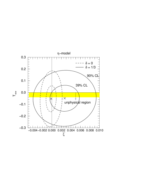
Figure 1: The 1-$\sigma$ and 90% CL allowed region on the $(\bar{\xi},T_{\rm new})$ plane in the $\eta$-model with $\delta=0$ and $1/3$. The shaded region ($T_{\rm new}<0$) corresponds to the unphysical region.

In Fig. 1, we show the 1-$\sigma$ and 90% CL allowed region on the $(\bar{\xi},T_{\rm new})$ plane in the $\eta$-model with $\delta=0$ and $1/3$ for $m_{H}=100~{}{\rm GeV}$.

The best fit results at $m_{H}=100~{}{\rm GeV}$ under the constraint $T_{\rm new}\geq 0$ are shown in Table 2. We can see from Table 2 that there is no noticeable improvement of the fit for the $\chi,\psi,\eta$ and $\nu$ models at $\delta=0$. The $\chi^{2}_{\rm min}$ remains almost the same as that of the SM, even though each model has two new free parameters, $T_{\rm new}$ and $\bar{\xi}$. The fit slightly improves for the leptophobic $\eta$-model ($\delta=1/3$) because of the smaller pull factor for the $R_{b}$ data. The probability of the fit, 18.7% CL, is still less than that of the SM, 26.2% CL, because the $\chi^{2}_{\rm min}$ reduces only 0.8 despite two additional free parameters.

We explore the whole range of the parameters, $\beta_{E}$ and $\delta$. In Fig. 2, we show the improvement in $\chi^{2}_{\rm min}$ over the SM value, $\chi^{2}_{\rm min}({\rm SM})=16.9$ (see Table 2):

$$\Delta\chi^{2}\equiv\chi_{\rm min}^{2}(\beta_{E},\delta)-\chi^{2}_{\rm min}({\rm SM}),$$ (4.27)

where $\chi^{2}_{\rm min}(\beta_{E},\delta)$ is evaluated at the specific value of $\beta_{E}$ and $\delta$ for $m_{H}=100~{}{\rm GeV}$.

Figure 2: Contour plot of $\Delta\chi^{2}\equiv\chi_{\rm min}^{2}(\beta,\delta)-\chi^{2}_{\rm min}({\rm SM})$ for $m_{H}=100~{}{\rm GeV}$. The mixing angle $\beta_{E}$ for the $\chi,\psi,\eta$ and $\nu$ models are shown by vertical dotted lines. The step of each contour is 0.2. The “$\times$” marks on the plot show the specific models listed in Table 8 in Sec. 5.

As we seen from Fig. 2, the $\chi^{2}_{\rm min}$ depends very mildly in the whole range of the $\beta_{E}$ and $\delta$ plane, except near the leptophobic $\eta$-model ($\beta_{E}=\tan^{-1}(\sqrt{5/3})$ and $\delta=1/3$) [10]. Even for the best choice of $\beta_{E}$ and $\delta$, the improvement in $\chi^{2}_{\rm min}$ is only 1.5 over the SM. Because each model has two additional parameters $T_{\rm new}$ and $\bar{\xi}$, we can conclude that no $Z^{\prime}$ model in this framework improves the fit over the SM. The “$\times$” marks plotted in Fig. 2 show the specific models which we will discuss in the next section.

4.2 Constraints from $Z$-pole + $m_{W}$ + LENC data

Next we find constraints on the contact term $g_{E}^{2}/c^{2}_{\chi}m_{Z_{2}}^{2}$ by including the low-energy data in addition to the $Z$-pole and $m_{W}$ data. Because $T_{\rm new}$ and $\bar{\xi}$ are already constrained severely by the $Z$-pole and $m_{W}$ data, only the contact terms proportional to $g_{E}^{2}/c_{\chi}^{2}m_{Z_{2}}^{2}$ contribute to the low-energy observables, except for the special case of the leptophobic $\eta$-model ($\delta=1/3$).

We summarize the results of the six-parameter fit for the $\psi,\chi,\eta$ and $\nu$ models:

(i) $\chi$-model

$$\!\!\!\!\left.\!\!\begin{array}[]{r c l c l c l }T_{\rm new}&\!\!=\!\!&\!\!-0.063\!\!&\!\!+\!\!&\!\!0.14x_{H}\!\!&\!\!\pm\!\!&\!\!0.11\!\!\!\!\\ \bar{\xi}&\!\!=\!\!&\!\!-0.00005\!\!&\!\!-\!\!&\!\!0.00006x_{H}\!\!&\!\!\pm\!\!&\!\!0.00044\!\!\!\\ g^{2}_{E}/c^{2}_{\chi}m^{2}_{Z_{2}}&\!\!=\!\!&\makebox[9.3894pt]{}\!\!0.26\!\!&\!\!+\!\!&\!\!0.01x_{H}\!\!&\!\!\pm\!\!&\!\!0.21\!\!\end{array}\right\}\rho_{\rm corr}\!=\!\left(\begin{array}[]{rrr}\!\!1.00\!&\!0.25\!&\!0.09\!\!\\ &\!1.00\!&\!0.15\!\\ &&\!1.00\!\end{array}\right)\!\!,\makebox[17.07164pt]{ }$$ (4.28g)

$$\chi^{2}_{\rm min}/({\rm d.o.f.})=(19.9+0.9x_{H})/(20),$$ (4.28h)

(ii) $\psi$-model

$$\!\!\!\!\left.\!\!\begin{array}[]{r c l c l c l }T_{\rm new}&\!\!=\!\!&\!\!-0.065\!\!&\!\!+\!\!&\!\!0.15x_{H}\!\!&\!\!\pm\!\!&\!\!0.11\!\!\\ \bar{\xi}&\!\!=\!\!&\!\!-0.00014\!\!&\!\!+\!\!&\!\!0.00012x_{H}\!\!&\!\!\pm\!\!&\!\!0.00050\!\!\!\\ g^{2}_{E}/c^{2}_{\chi}m^{2}_{Z_{2}}&\!\!=\!\!&\!\!\makebox[9.3894pt]{}1.66\!\!&\!\!+\!\!&\!\!0.19x_{H}\!\!&\!\!\pm\!\!&\!\!2.90\!\!\end{array}\right\}\rho_{\rm corr}\!=\!\left(\begin{array}[]{rrr}\!\!1.00\!&\!0.19\!&\!0.07\!\!\\ &\!1.00\!&\!0.03\!\\ &&\!1.00\!\end{array}\right)\!\!,\makebox[17.07164pt]{ }$$ (4.29g)

$$\chi^{2}_{\rm min}/({\rm d.o.f.})=(21.1+0.8x_{H})/(20),$$ (4.29h)

(iii) $\eta$-model

$$\!\!\!\!\left.\!\!\begin{array}[]{r c l c l c l }T_{\rm new}\!&\!\!\!=\!\!&\!\!-0.074\!\!&\!\!+\!\!&\!\!0.14x_{H}\!\!&\!\!\pm\!\!&\!\!0.11\!\!\!\\ \bar{\xi}\!&\!\!\!=\!\!&\!\!-0.00038\!\!&\!\!-\!\!&\!\!0.00063x_{H}\!\!&\!\!\pm\!\!&\!\!0.00106\!\!\!\!\\ g^{2}_{E}/c^{2}_{\chi}m^{2}_{Z_{2}}\!&\!\!=\!\!&\!\!-0.62\!\!&\!\!+\!\!&\!\!0.08x_{H}\!\!&\!\!\pm\!\!&\!\!0.87\!\!\!\end{array}\right\}\!\rho_{\rm corr}\!=\!\left(\begin{array}[]{rrr}\!\!1.00\!&\!0.06\!&\!-0.05\!\!\\ &\!\!1.00\!&\!-0.22\!\!\\ &&\!1.00\!\end{array}\right)\!\!,\makebox[17.07164pt]{ }$$ (4.30g)

$$\chi^{2}_{\rm min}/({\rm d.o.f.})=(20.8+0.5x_{H})/(20),$$ (4.30h)

(iv) $\nu$-model

$$\!\!\!\!\left.\!\!\begin{array}[]{r c l c l c l }T_{\rm new}&\!\!=\!\!&\!\!-0.061\!\!&\!\!+\!\!&\!\!0.15x_{H}\!\!&\!\!\pm\!\!&\!\!0.11\!\!\\ \bar{\xi}&\!\!=\!\!&\!\!\makebox[9.3894pt]{}0.00010\!\!&\!\!+\!\!&\!\!0.00006x_{H}\!\!&\!\!\pm\!\!&\!\!0.00041\!\!\!\!\\ g^{2}_{E}/c^{2}_{\chi}m^{2}_{Z_{2}}\!&\!\!=\!\!&\!\!-0.65\!\!&\!\!+\!\!&\!\!0.04x_{H}\!\!&\!\!\pm\!\!&\!\!0.54\!\!\end{array}\right\}\rho_{\rm corr}\!=\!\left(\begin{array}[]{rrr}\!\!1.00\!&\!0.21\!&\!0.07\!\\ &\!1.00\!&\!0.03\!\\ &&\!1.00\!\end{array}\right)\!\!,\makebox[17.07164pt]{ }$$ (4.31g)

$$\chi^{2}_{\rm min}/({\rm d.o.f.})=(20.1+0.8x_{H})/(20).$$ (4.31h)

The contact term $g_{E}^{2}/c^{2}_{\chi}m_{Z_{2}}^{2}$ in the $\psi$ and $\eta$ models is consistent with zero in 1-$\sigma$ level. Both the best fit and the 1-$\sigma$ error of the parameters $T_{\rm new}$ and $\bar{\xi}$ in all the $Z^{\prime}$ models are slightly affected by including the LENC data: The best fit value of $T_{\rm new}$ in all the $Z^{\prime}$ models cannot be positive even for the $m_{H}=150~{}{\rm GeV}$ $(x_{H}=0.41)$. Since the leptophobic $\eta$-model does not have the contact term, the low-energy data constrain the same parameters $T_{\rm new}$ and $\bar{\xi}$. After taking into account both the high-energy and low-energy data, we find

1. leptophobic $\eta$ model ($\delta=1/3$)

   $$\begin{array}[]{l}\left.\begin{array}[]{lrl}T_{\rm new}&=&-0.074+0.148x_{H}\pm 0.110\\ \bar{\xi}&=&\hphantom{-}0.00157+0.00019x_{H}\pm 0.00279\end{array}\right\}\rho_{\rm corr}=0.02,\\ \chi^{2}_{\rm min}/({\rm d.o.f.})=(21.2+1.0x_{H})/(21).\end{array}$$ (4.36)

The allowed range of $\bar{\xi}$ is slightly severe as compared to eq. (4.26).

The best fit results for $m_{H}=100~{}{\rm GeV}$ under the condition $T_{\rm new}\geq 0$ are shown in Table 3. It is noticed that the best fit values for the weak charge of cesium atom ${}^{133}_{55}Cs$ in the $\chi,\eta$ and $\nu$ models are quite close to the experimental data. These models lead to $\Delta\chi^{2}=-1.8$ ($\chi$), $-0.8$ $(\eta)$ and $-1.6$ $(\nu)$. No other noticeable point is found in the table.

Figure 3: Contour plot of the 95% CL lower mass limit of the $Z_{2}$ boson obtained from the LENC experiments for $g_{E}=g_{Y}$ and $m_{H}=100~{}{\rm GeV}$. The vertical dotted lines correspond to the $\chi,\psi,\eta$ and $\nu$ models. The limits are given in the unit of GeV. The “$\times$” marks on the plot show the specific models listed in Table 8 in Sec. 5.

The above constraints on $g_{E}^{2}/c^{2}_{\chi}m_{Z_{2}}^{2}$ from the LENC data give the lower mass bound of the heavier mass eigenstate $Z_{2}$ in the $Z^{\prime}$ models except for the leptophobic $\eta$-model. In Fig. 3, the contour plot of the 95% CL lower mass limit of $Z_{2}$ boson from the LENC experiments are shown on the $(\beta_{E},\delta)$ plane by setting $g_{E}=g_{Y}$ and $m_{H}=100~{}{\rm GeV}$ under the condition $m_{Z_{2}}\geq 0$. In practice, we obtain the 95% CL lower limit of the $Z_{2}$ boson mass $m_{95}$ in the following way:

$$0.05=\frac{\int^{\infty}_{m_{95}}dm_{Z_{2}}P(m_{Z_{2}})}{\int^{\infty}_{0}dm_{Z_{2}}P(m_{Z_{2}})},$$ (4.37)

where we assume that the probability density function $P(m_{Z_{2}})$ is proportional to ${\rm exp}(-\chi^{2}(m_{Z_{2}})/2)$.

We can read off from Fig. 3 that the lower mass bound of the $Z_{2}$ boson in the $\psi$ model at $\delta=0$ is much weaker than those of the other $Z^{\prime}$ models. It has been pointed out that the most stringent constraint on the contact term is the APV measurement of cesium atom [6]. Since all the SM matter fields in the $\psi$ model have the same ${\rm U(1)^{\prime}}$ charge (see Table 1), the couplings of contact interactions are Parity conserving, which makes constraint from the APV measurement useless. We also find in Fig. 3 that the lower mass bound of the $Z_{2}$ boson disappears near the leptophobic $\eta$-model ($\beta_{E}=\tan^{-1}(\sqrt{5/3})$ and $\delta=1/3$) [10].

We summarize the 95% CL lower bound on $m_{Z_{2}}$ for the $\chi,\psi,\eta$ and $\nu$ models ($\delta=0$) in Table 5. For comparison, we also show the lower bound of $m_{Z_{2}}$ in the previous study [36] in the same table. The bounds on the $Z_{\chi}$ and $Z_{\nu}$ masses are more severely constrained as compared to ref. [36]. Although we used the latest electroweak data, our result for the $Z_{\psi}$ boson mass is somewhat weaker than that of ref. [36]. In the analysis of ref. [36], the $e^{+}e^{-}\rightarrow\mu^{+}\mu^{-},\tau^{+}\tau^{-}$ data below the $Z$ pole are also used besides the $Z$-pole, $m_{W}$ and the LENC data. As we mentioned before, the lower mass bound of the $Z^{\prime}$ boson is obtained from the LENC data, not from the $Z$-pole data. Because the APV measurement which is most stringent constraint in the LENC data does not well constrain the $\psi$ model, it is expected that the $e^{+}e^{-}$ annihilation data below the $Z$-pole play an important role to obtain the bound of $Z_{\psi}$ boson mass.

Table 5: The 95% CL lower bound of $m_{Z_{2}}$ (GeV) in the $\chi,\psi,\eta$ and $\nu$ models ($\delta=0$) for $g_{E}=g_{Y}$ and $m_{H}=100~{}{\rm GeV}$. The results of previous study [36] and of recent direct search [37] are shown for comparison.

	$\chi$	$\psi$	$\eta$	$\nu$
Our results	451	136	317	284
Langacker et al.  [36]	330	170	220	—
direct search [37]	595	590	620	—

Our results in Table 5 are also slightly weaker than those in ref. [6]. The results in ref. [6] have been obtained without including the $Z$-$Z^{\prime}$ mixing effects and by setting $m_{t}=175~{}{\rm GeV},m_{H}=100~{}{\rm GeV},x_{\alpha}=0$ and $T_{\rm new}=0$.

4.3 Lower mass bound of $Z_{2}$ boson

We have found that the $Z$-pole, $m_{W}$ and the LENC data constrain ($T_{\rm new},\bar{\xi}$), $T_{\rm new}$ and $g_{E}^{2}/c^{2}_{\chi}m_{Z_{2}}^{2}$, respectively. We can see from eq. (2.23) that, for a given $\zeta$, constraints on $T_{\rm new},\bar{\xi}$ and $g_{E}^{2}/c^{2}_{\chi}m_{Z_{2}}^{2}$ can be interpreted as the bound on $m_{Z_{2}}$. We show the 95% CL lower mass bound of the $Z_{2}$ boson for $m_{H}=100~{}{\rm GeV}$ in four $Z^{\prime}$ models as a function of $\zeta$. The bound is again found under the condition $m_{Z_{2}}\geq 0$. Results are shown in Fig. 4.(a) $\sim$ 4.(d) for the $\chi,\psi,\eta,\nu$ models, respectively. The lower bound from the $Z$-pole and $m_{W}$ data, and that from the LENC data are separately plotted in the same figure. In order to see the $g_{E}$-dependence of the $m_{Z_{2}}$ bound explicitly, we show the lower mass bound for the combination $m_{Z_{2}}g_{Y}/g_{E}$. We can read off from Fig. 4 that the bound on $m_{Z_{2}}g_{Y}/g_{E}$ is approximately independent of $g_{E}$ for $g_{E}/g_{Y}=0.5\sim 2.0$ in each model.

Figure 4: The 95% CL lower mass limit of $Z_{2}$ in the $\chi$, $\psi$, $\eta$ and $\nu$ models for $m_{H}=100~{}{\rm GeV}$. The $Z_{2}$ boson mass is normalized by $g_{E}/g_{Y}$. Constraints from $Z$-pole experiments and LENC experiments are separately shown. The results of the direct search at Tevatron [37] for the $\chi,\psi$ and $\eta$ models are also shown.

As we expected from the formulae for $T_{\rm new}$ and $\bar{\xi}$ in the small mixing limit (eq. (2.2)), the $Z_{2}$ mass is unbounded from the $Z$-pole data at $\zeta=0$. For models with very small $\zeta$, the lower bound on $m_{Z_{2}}$, therefore, comes from the LENC experiments and the direct search experiment at Tevatron. For comparison, we plot the 95% CL lower bound on $m_{Z_{2}}$ obtained from the direct search experiment [37] in Fig. 4. In the direct search experiment, the $Z^{\prime}$ decays into the exotic particles, e.g., the decays into the light right-handed neutrinos which are expected for some models, are not taken into account. We summarize the 95% CL lower bound on $m_{Z_{2}}$ for the $\chi,\psi,\eta$ and $\nu$ models ($\delta=0$) obtained from the low-energy data and the direct search experiment [37] in Table 5.

The lower bound of $m_{Z_{2}}$ is affected by the Higgs boson mass through the $T$ parameter. As we seen from eqs. (4.6) $\sim$ (4.21), $T_{\rm new}$ tends to be in the physical region ($T_{\rm new}\geq 0$) for large $m_{H}$ $(x_{H})$. Then, we find that the large Higgs boson mass decreases the lower bound of $m_{Z_{2}}$. For $\zeta=1$, the lower $m_{Z_{2}}$ bound in the $\chi,\psi,\nu$ ($\eta$) models for $m_{H}=150~{}{\rm GeV}$ is weaker than that for $m_{H}=100~{}{\rm GeV}$ about 7% (11%). On the other hand, the Higgs boson with $m_{H}=80~{}{\rm GeV}$ makes the lower $m_{Z_{2}}$ bound in all the $Z^{\prime}$ models severe about 5% as compared to the case for $m_{H}=100~{}{\rm GeV}$. Because $T_{\rm new}$ and $\bar{\xi}$ are proportional to $\zeta^{2}$ and $\zeta$, respectively (see eq. (2.2)), and it is unbounded at $|\zeta|\simeq 0$, the lower bound of $m_{Z_{2}}$ may be independent of $m_{H}$ in the small $|\zeta|$ region. The $m_{H}$-dependence of the lower mass bound obtained from the LENC data is safely negligible.

It should be noted that, at $\zeta=0$, only the leptophobic $\eta$-model ($\delta=1/3$) is not constrained from both the $Z$-pole and the low-energy data. The precise analysis and discussion for the lower mass bound of the $Z_{2}$ boson in the leptophobic $\eta$-model can be found in ref. [38]. It is shown in ref. [38] that the $\zeta$-dependence of the lower mass bound is slightly milder than that of the $\eta$-model with $\delta=0$ in Fig. 4.(c).

It has been discussed that the presence of $Z_{2}$ boson whose mass is much heavier than the SM $Z$ boson mass, say 1 TeV, may lead to a find-tuning problem to stabilize the electroweak scale against the ${\rm U(1)^{\prime}}$ scale [39]. The $Z_{2}$ boson with $m_{Z_{2}}\leq 1~{}{\rm TeV}$ for $g_{E}=g_{Y}$ is allowed by the electroweak data only if $\zeta$ satisfies the following condition:

$$\begin{array}[]{ll}-0.6~{}{\hbox to0.0pt{\lower 3.5pt\hbox{$\mathchar 0\relax\sim$}\hss}\raise 1.0pt\hbox{$<$}}\,\zeta~{}{\hbox to0.0pt{\lower 3.5pt\hbox{$\mathchar 0\relax\sim$}\hss}\raise 1.0pt\hbox{$<$}}\,+0.3&~{}~{}{\rm for~{}the}~{}\chi,\psi,\nu~{}{\rm models},\\ -0.7~{}{\hbox to0.0pt{\lower 3.5pt\hbox{$\mathchar 0\relax\sim$}\hss}\raise 1.0pt\hbox{$<$}}\,\zeta~{}{\hbox to0.0pt{\lower 3.5pt\hbox{$\mathchar 0\relax\sim$}\hss}\raise 1.0pt\hbox{$<$}}\,+0.6&~{}~{}{\rm for~{}the}~{}\eta~{}{\rm model}.\end{array}$$ (4.40)

In principle, the parameter $\zeta$ is calculable, together with the gauge coupling $g_{E}$, once the particle spectrum of the $E_{6}$ model is specified. In the next section, we calculate the $\zeta$ parameter in several $E_{6}$ $Z^{\prime}$ models.

5 Light $Z^{\prime}$ boson in minimal SUSY $E_{6}$-models

It is known that the gauge couplings are not unified in the $E_{6}$ models with three generations of 27. In order to guarantee the gauge coupling unification, a pair of weak-doublets, $H^{\prime}$ and $\overline{H^{\prime}}$, should be added into the particle spectrum at the electroweak scale [40]. They could be taken from ${\bf 27}+{\bf\overline{27}}$ or the adjoint representation 78. The ${\rm U(1)^{\prime}}$ charges of the additional weak doublets should have the same magnitude and opposite sign, $a$ and $-a$, to cancel the ${\rm U(1)^{\prime}}$ anomaly. In addition, a pair of the complete SU(5) multiplet such as ${\bf 5+\overline{5}}$ can be added without spoiling the unification of the gauge couplings [10, 40].

The minimal $E_{6}$ model which have three generations of 27 and a pair ${\bf 2}+{\bf\overline{2}}$ depends in principle on the three cases; $H^{\prime}$ has the same quantum number as $L$ or $H_{d}$ of 27, or $\overline{H_{u}}$ of ${\bf\overline{27}}$. All three cases will be studied below.

Table 6: Charge assignment for the extra weak doublets in the minimal $E_{6}$ model and the $\eta_{\rm BKM}$ model of ref. [10]. The symbol $a_{i}(-a_{i})$ for $i=\chi,\psi,\eta,\nu$ are the ${\rm U(1)^{\prime}}$ charge of $L$ or $H_{d}$ ($H_{u}$).

	field	$Y$	$2\sqrt{6}Q_{\chi}$	$\sqrt{72/5}Q_{\psi}$	$Q_{\eta}$	$Q_{\nu}$
minimal model	$H^{\prime}$	$-\frac{1}{2}$	$\hphantom{-}a_{\chi}$	$\hphantom{-}a_{\psi}$	$\hphantom{-}a_{\eta}$	$\hphantom{-}a_{\nu}$
	$\overline{H}^{\prime}$	$+\frac{1}{2}$	$-a_{\chi}$	$-a_{\psi}$	$-a_{\eta}$	$-a_{\nu}$
$\eta_{\rm BKM}$ model [10]	$H^{\prime}_{1}$	$-\frac{1}{2}$			$\hphantom{-}1$
	$\overline{H_{1}}$	$+\frac{1}{2}$			$-1$
	$H^{\prime}_{2}$	$-\frac{1}{2}$			$\hphantom{-}1$
	$\overline{H_{2}}$	$+\frac{1}{2}$			$-1$
	$D^{\prime}$	$-\frac{1}{3}$			$\hphantom{-}\frac{2}{3}$
	$\overline{D^{\prime}}$	$+\frac{1}{3}$			$-\frac{2}{3}$

The hypercharge and ${\rm U(1)^{\prime}}$ charge of the extra weak doublets for the $\chi,\psi,\eta,\nu$ models are listed in Table 6. For comparison, we also show those in the model of Babu et al.  [10], where two pairs of ${\bf 2+\overline{2}}$ from 78 and a pair of ${\bf 3+\overline{3}}$ from ${\bf 27+\overline{27}}$ are introduced to achieve the quasi-leptophobity at the weak scale.

Let us recall the definition of $\zeta$;

$$\zeta=\frac{g_{Z}}{g_{E}}\frac{m_{ZZ^{\prime}}^{2}}{m_{Z}^{2}}-\delta.$$ (5.1)

In the minimal model, the following eight scalar-doublets can develop VEV to give the mass terms $m_{Z}^{2}$ and $m_{ZZ^{\prime}}^{2}$ in eq. (2.8): three generations of $H_{u},H_{d}$, and an extra pair, $H^{\prime}$ and $\overline{H^{\prime}}$. Then, $m_{Z}^{2}$ and $m_{ZZ^{\prime}}^{2}$ are written in terms of their VEVs as

$$m_{Z}^{2} = \frac{1}{2}g_{Z}^{2}\biggl{[}\sum_{i=1}^{3}\biggl{\{}\langle H_{u}^{i}\rangle^{2}+\langle H_{d}^{i}\rangle^{2}\biggr{\}}+\langle H^{\prime}\rangle^{2}+\langle\overline{H^{\prime}}\rangle^{2}\biggr{]},$$ (5.2a)

$$m_{ZZ^{\prime}}^{2} = \!g_{Z}g_{E}\biggl{[}\sum_{i=1}^{3}\biggl{\{}-Q_{E}^{H_{u}}\langle H_{u}^{i}\rangle^{2}+Q_{E}^{H_{d}}\langle H_{d}^{i}\rangle^{2}\biggr{\}}+Q_{E}^{H^{\prime}}\langle H^{\prime}\rangle^{2}-Q_{E}^{\overline{H^{\prime}}}\langle\overline{H^{\prime}}\rangle^{2}\biggr{]}\!,$$ (5.2b)

where $i$ is the generation index. The third component of the weak isospin $I_{3}$ for the Higgs fields are

$$I_{3}(H_{d})=I_{3}(H^{\prime})=-I_{3}(H_{u})=-I_{3}(\overline{H^{\prime}})=1/2.$$ (5.3)

Taking account of the ${\rm U(1)^{\prime}}$ charges of the extra Higgs doublets, $Q_{E}^{H^{\prime}}=-Q_{E}^{\overline{H^{\prime}}}$, we find from eq. (5.1)

$$\zeta = 2\frac{\displaystyle{\sum_{i=1}^{3}}\biggl{\{}-Q_{E}^{H_{u}}\langle H_{u}^{i}\rangle^{2}+Q_{E}^{H_{d}}\langle H_{d}^{i}\rangle^{2}\biggr{\}}+Q_{E}^{H^{\prime}}\biggl{(}\langle H^{\prime}\rangle^{2}+\langle\overline{H^{\prime}}\rangle^{2}\biggr{)}}{\displaystyle{\sum_{i=1}^{3}}\biggl{\{}\langle H_{u}^{i}\rangle^{2}+\langle H_{d}^{i}\rangle^{2}\biggr{\}}+\langle H^{\prime}\rangle^{2}+\langle\overline{H^{\prime}}\rangle^{2}}-\delta.$$ (5.4)

We note here that the observed $\mu$-decay constant leads to the following sum rule

$$v_{u}^{2}+v_{d}^{2}+v_{H^{\prime}}^{2}+v_{\overline{H^{\prime}}}^{2}\equiv v^{2}=\frac{1}{\sqrt{2}G_{F}}\approx(246~{}{\rm GeV})^{2},$$ (5.5)

where

$$\left.\begin{array}[]{rr}\displaystyle{\sum_{i=1}^{3}\langle H_{u}^{i}\rangle^{2}=\frac{v_{u}^{2}}{2},}&\displaystyle{\sum_{i=1}^{3}\langle H_{d}^{i}\rangle^{2}=\frac{v_{d}^{2}}{2},}\\ \displaystyle{\langle H^{\prime}\rangle^{2}=\frac{v_{H^{\prime}}^{2}}{2},}&\displaystyle{\langle\overline{H^{\prime}}\rangle^{2}=\frac{v_{\overline{H^{\prime}}}^{2}}{2}}.\end{array}\right.$$ (5.8)

By further introducing the notation

$$\tan\beta = \frac{v_{u}}{v_{d}},$$ (5.9a)

$$x^{2} = \frac{v_{H^{\prime}}^{2}+v_{\overline{H^{\prime}}}^{2}}{v^{2}},$$ (5.9b)

we can express eq. (5.4) as

$$\zeta = 2\biggl{\{}-Q_{E}^{H_{u}}(1-x^{2})\sin^{2}\beta+Q_{E}^{H_{d}}(1-x^{2})\cos^{2}\beta+Q_{E}^{H^{\prime}}x^{2}\biggr{\}}-\delta.$$ (5.10)

Because $H^{\prime}$ and $\overline{H^{\prime}}$ are taken from 27 + $\bf\overline{27}$, the ${\rm U(1)^{\prime}}$ charge of $H^{\prime}$, $Q_{E}^{H^{\prime}}$, is identified with that of $L$, $H_{d}$ or $\overline{H_{u}}$.

Among all the models, only in the $\chi$-model one can have smaller number of matter particles. In the $\chi$-model, three generations of the matter fields 16 and a pair of Higgs doublets make the model anomaly free. In this case, $\zeta$ is found to be independent of $\tan\beta$:

$$\zeta = 2\frac{Q_{E}^{H_{d}}-Q_{E}^{H_{u}}\tan^{2}\beta}{1+\tan^{2}\beta}-\delta$$ (5.11a)

$$= 2Q_{E}^{H_{d}}-\delta.$$ (5.11b)

Table 7: Coefficients of the 1-loop $\beta$-functions for the gauge couplings in the MSSM, the minimal $E_{6}$ models and the $\eta_{\rm BKM}$ model [10]. The model $\chi(16)$ has three generations of ${\bf 16}$ and a pair ${\bf 2}+{\bf\overline{2}}$. The model $\chi(27)$ and $\psi,\eta,\nu$ have three generations of ${\bf 27}$ and a pair ${\bf 2}+{\bf\overline{2}}$.

	MSSM	$\chi(16)$	$\chi(27)$	$\psi$	$\eta$	$\nu$	$\eta_{\rm BKM}$ [10]
$b_{1}$	$\frac{33}{5}$	$\hphantom{-}\frac{33}{5}$	$\frac{48}{5}$	$\frac{48}{5}$	$\frac{48}{5}$	$\frac{48}{5}$	$\frac{53}{5}$
$b_{2}$	1	-1	4	4	4	4	-5
$b_{3}$	$-3$	$-3$	0	0	0	0	-1
$b_{E}$	—	$6+\frac{a^{2}}{10}$	$9+\frac{a^{2}}{10}$	$9+\frac{a^{2}}{6}$	$9+\frac{12}{5}a^{2}$	$9+\frac{12}{5}a^{2}$	$\frac{77}{5}$
$b_{1E}$	—	$-\sqrt{\frac{3}{50}}a$	$-\sqrt{\frac{3}{50}}a$	$-\sqrt{\frac{1}{10}}a$	$-\frac{6}{5}a$	$-\frac{6}{5}a$	$-\frac{16}{5}$

Let us now examine the kinetic mixing parameter $\delta$ in each model. The boundary condition of $\delta$ at the GUT scale is $\delta=0$. The non-zero kinetic mixing term can arise at low-energy scale through the following RGEs:

$$\frac{d}{dt}\alpha_{i} = \frac{1}{2\pi}b_{i}\alpha_{i}^{2},$$ (5.12a)

$$\frac{d}{dt}\alpha_{4} = \frac{1}{2\pi}(b_{E}+2b_{1E}\delta+b_{1}\delta^{2})\alpha_{4}^{2},$$ (5.12b)

$$\frac{d}{dt}\delta = \frac{1}{2\pi}(b_{1E}+b_{1}\delta)\alpha_{1},$$ (5.12c)

where $i=1,2,3$ and $t=\ln\mu$. We define $\alpha_{1}$ and $\alpha_{4}$ as

$$\alpha_{1}\equiv\frac{5}{3}\frac{g_{Y}^{2}}{4\pi},~{}~{}~{}~{}~{}~{}~{}\alpha_{4}\equiv\frac{5}{3}\frac{g_{E}^{2}}{4\pi}.$$ (5.13)

The coefficients of the $\beta$-functions for $\alpha_{1},\alpha_{4}$ and $\delta$ are:

$$b_{1}=\frac{3}{5}{\rm Tr}(Y^{2}),~{}~{}~{}~{}b_{E}=\frac{3}{5}{\rm Tr}(Q_{E}^{2}),~{}~{}~{}~{}b_{1E}=\frac{3}{5}{\rm Tr}(YQ_{E}).$$ (5.14)

From eq. (5.12c), we can clearly see that the non-zero $\delta$ is generated at the weak scale if $b_{1E}\neq 0$ holds. In Table 7, we list $b_{1},b_{E}$ and $b_{1E}$ in the minimal $\chi,\psi,\eta,\nu$ models and the $\eta_{\rm BKM}$ model [10]. As explained above, the $\chi(16)$ model has three generations of 16, and the $\chi(27)$ model has three generations of 27. We can see from Table 7 that the magnitudes of the differences $b_{1}-b_{2}$ and $b_{2}-b_{3}$ are common among all the models including the minimal supersymmetric SM. This guarantees the gauge coupling unification at $\mu=m_{GUT}\simeq 10^{16}~{}{\rm GeV}$.

Table 8: Predictions for $g_{E}$ and $\delta$ at $\mu=m_{Z_{1}}$ in the minimal models and the $\eta_{\rm BKM}$ model [10]. The ${\rm U(1)}_{Y}$ gauge coupling $g_{Y}$ is fixed as $g_{Y}=0.36$.

model	$a$	$g_{E}$	$g_{E}/g_{Y}$	$\delta$
$\chi(16)$	$\hphantom{-}3$	$\hphantom{-}0.353$	$0.989$	$\hphantom{-}0.066$
	$-2$	$\hphantom{-}0.361$	$1.010$	$-0.044$
$\chi(27)$	$\hphantom{-}3$	$\hphantom{-}0.353$	$0.989$	$\hphantom{-}0.066$
	$-2$	$\hphantom{-}0.361$	$1.010$	$-0.044$
$\psi$	$\hphantom{-}1$	$\hphantom{-}0.364$	$1.020$	$\hphantom{-}0.028$
	$\hphantom{-}2$	$\hphantom{-}0.356$	$0.999$	$\hphantom{-}0.056$
	$-2$	$\hphantom{-}0.356$	$0.999$	$-0.056$
$\eta$	$\hphantom{-}1/6$	$\hphantom{-}0.366$	$1.025$	$\hphantom{-}0.018$
	$-2/3$	$\hphantom{-}0.351$	$0.982$	$-0.071$
$\nu$	$\hphantom{-}\sqrt{1/6}$	$\hphantom{-}0.361$	$1.010$	$\hphantom{-}0.044$
	$-\sqrt{3/8}$	$\hphantom{-}0.353$	$0.989$	$-0.066$
$\eta_{\rm BKM}$ [10]	—	$\hphantom{-}0.308$	$0.862$	$\hphantom{-}0.286$

It is straightforward to obtain $g_{E}(m_{Z_{1}})$ and $\delta(m_{Z_{1}})$ for each model. The analytical solutions of eqs. (5.12a)$\sim$ (5.12c) are as follows:

$$\frac{1}{\alpha_{i}(m_{Z_{1}})} = \frac{1}{\alpha_{GUT}}+\frac{1}{2\pi}b_{i}\ln\frac{m_{GUT}}{m_{Z_{1}}},$$ (5.15a)

$$\delta(m_{Z_{1}}) = -\frac{b_{1E}}{b_{1}}\biggl{(}1-\frac{\alpha_{1}(m_{Z_{1}})}{\alpha_{GUT}}\biggr{)},$$ (5.15b)

$$\frac{1}{\alpha_{4}(m_{Z_{1}})} = \frac{1}{\alpha_{GUT}}+\biggl{\{}\frac{b_{E}}{b_{1}}-\biggl{(}\frac{b_{1E}}{b_{1}}\biggr{)}^{2}\biggr{\}}\biggl{\{}\frac{1}{\alpha_{1}(m_{Z_{1}})}-\frac{1}{\alpha_{GUT}}\biggr{\}}$$ (5.15c)

$$-\biggl{(}\frac{b_{1E}}{b_{1}}\biggr{)}^{2}\frac{\alpha_{1}(m_{Z_{1}})-\alpha_{GUT}}{\alpha_{GUT}^{2}},$$

where $\alpha_{GUT}$ denotes the unified gauge coupling at $\mu=m_{GUT}$. In our calculation, $\alpha_{3}(m_{Z_{1}})=0.118$ and $\alpha(m_{Z_{1}})=e^{2}(m_{Z_{1}})/4\pi=1/128$ are used as example. These numbers give $g_{Y}(m_{Z_{1}})=0.357$. We summarize the predictions for $g_{E}$ and $\delta$ at $\mu=m_{Z_{1}}$ in the minimal $E_{6}$ models and the $\eta_{\rm BKM}$ model in Table 8. In all the minimal models, the ratio $g_{E}/g_{Y}$ is approximately unity and $|\delta|$ is smaller than about 0.07. On the other hand, the $\eta_{\rm BKM}$ model predicts

Table 9: Predictions for the effective $Z$-$Z^{\prime}$ mixing parameter $\zeta$ in the minimal $\chi,\psi,\eta,\nu$ and the $\eta_{\rm BKM}$ model for $x^{2}=0$ and $0.5$, and $\tan\beta=2$ and $30$.

		$x^{2}=0$		$x^{2}=0.5$
		$\tan\beta$		$\tan\beta$
	$a$	2	30	2	30
$\chi$	$\hphantom{-}3$	$-0.88$		$0.14$
	$-2$	$-0.77$
$\psi$	$\hphantom{-}1$	$\hphantom{-}0.60$	$\hphantom{-}1.02$	$\hphantom{-}0.55$	$\hphantom{-}0.76$
	$\hphantom{-}2$	$\hphantom{-}0.58$	$\hphantom{-}1.00$	$\hphantom{-}0.79$	$\hphantom{-}1.00$
	$-2$	$\hphantom{-}0.69$	$\hphantom{-}1.11$	$-0.16$	$\hphantom{-}0.06$
$\eta$	$\hphantom{-}1/6$	$-1.02$	$-1.35$	$-0.35$	$-0.52$
	$-2/3$	$-0.93$	$-1.26$	$-1.11$	$-1.26$
$\nu$	$\hphantom{-}\sqrt{1/6}$	$\hphantom{-}0.36$	$\hphantom{-}0.77$	$\hphantom{-}0.57$	$\hphantom{-}0.77$
	$-\sqrt{3/8}$	$\hphantom{-}0.47$	$\hphantom{-}0.88$	$-0.34$	$-0.14$
$\eta_{\rm BKM}$	—	$-1.29$	$-1.62$	$-1.79$	$-1.95$

$g_{E}/g_{Y}\sim 0.86$ and $\delta\sim 0.29$, which is close to the leptophobic-$\eta$ model at $\delta=1/3$. In Figs. 2 and 3, we show the predictions of all the models by “$\times$” symbol.

Next, we estimate the parameter $\zeta$ for several sets of $\tan\beta$ and $x$. In Table 9, we show the predictions for $\zeta$ in the minimal $\chi,\psi,\eta,\nu$ models and the $\eta_{\rm BKM}$ model. The results are shown for $\tan\beta=2$ and $30$, and $x^{2}=0$ and $0.5$. We find from the table that the parameter $\zeta$ is in the range $|\zeta|~{}{\hbox to0.0pt{\lower 3.5pt\hbox{$\mathchar 0\relax\sim$}\hss}\raise 1.0pt\hbox{$<$}}\,1.35$ for all the models except for the $\eta_{\rm BKM}$ model, where the predicted $\zeta$ lies between $-2.0$ and $-1.2$. It is shown in Fig. 4 that $m_{Z_{2}}g_{Y}/g_{E}$ is approximately independent of $g_{E}/g_{Y}$. Actually, we find in Table 8 and Table 9 that the predicted $|\delta|$ is smaller than about 0.1 and $g_{E}/g_{Y}$ is quite close to unity in all the minimal models. We can, therefore, read off from Fig. 4 the lower bound of $m_{Z_{2}}$ in the minimal models at $g_{E}=g_{Y}$. In Table 10, we summarize the 95% CL lower $m_{Z_{2}}$ bound for the minimal $\chi,\psi,\eta,\nu$ models and the $\eta_{\rm BKM}$ model which correspond to the predicted $\zeta$ in Table 9.

Table 10: Summary of the 95% CL lower bound of $m_{Z_{2}}$ (GeV) which corresponds to the predicted $\zeta$ in Table 9.

		$x^{2}=0$		$x^{2}=0.5$
		$\tan\beta$		$\tan\beta$
	$a$	$~{}~{}~{}~{}~{}~{}2$	$~{}~{}~{}~{}30$	$~{}~{}~{}~{}~{}~{}2$	$~{}~{}~{}~{}30$
$\chi$	$\hphantom{-}3$	$1330$		$620$
	$-2$	$1230$
$\psi$	$\hphantom{-}1$	$1290$	$1800$	$1220$	$1480$
	$\hphantom{-}2$	$1250$	$1750$	$1510$	$1750$
	$-2$	$1380$	$1890$	$520$	$370$
$\eta$	$+1/6$	$1330$	$1690$	$620$	$790$
	$-2/3$	$1230$	$1590$	$1410$	$1590$
$\nu$	$-\sqrt{3/8}$	$1180$	$1720$	$800$	$520$
	$+\sqrt{1/6}$	$1030$	$1580$	$1320$	$1580$
$\eta_{\rm BKM}$	—	$1520$	$1930$	$2150$	$2360$

Most of the lower mass bounds in Table 10 exceed 1 TeV. The $Z_{2}$ boson with $m_{Z_{2}}\sim O(1~{}{\rm TeV})$ should be explored at the future collider such as LHC. The discovery limit of the $Z^{\prime}$ boson in the $E_{6}$ models at LHC is expected as [41]

$$\begin{array}[]{cccc}\hline\cr\chi&\psi&\eta&\nu\\ \hline\cr 3040&2910&2980&***\\ \hline\cr\end{array}$$ (5.18)

All the lower bounds of $m_{Z_{2}}$ listed in Table 10 are smaller than 2 TeV and they are, therefore, in the detectable range of LHC. But, it should be noticed that most of them ($1~{}{\rm TeV}~{}{\hbox to0.0pt{\lower 3.5pt\hbox{$\mathchar 0\relax\sim$}\hss}\raise 1.0pt\hbox{$<$}}\,m_{Z_{2}}$) may require the fine-tuning to stabilize the electroweak scale against the ${\rm U(1)^{\prime}}$ scale [39].

The lower bound of the $Z_{2}$ boson mass in the $\eta_{\rm BKM}$ model for the predicted $\zeta$ can be read off from Fig. 2 in ref. [38]. Because somewhat large $\zeta$ is predicted in the $\eta_{\rm BKM}$ model, $1~{}{\hbox to0.0pt{\lower 3.5pt\hbox{$\mathchar 0\relax\sim$}\hss}\raise 1.0pt\hbox{$<$}}\,|\zeta|$, the lower mass bound is also large as compared to the minimal models.

6 Summary

We have studied constraints on $Z^{\prime}$ bosons in the SUSY $E_{6}$ models. Four $Z^{\prime}$ models — the $\chi,\psi,\eta$ and $\nu$ models are studied in detail. The presence of the $Z^{\prime}$ boson affects the electroweak processes through the effective $Z$-$Z^{\prime}$ mass mixing angle $\bar{\xi}$, a tree level contribution $T_{\rm new}$ which is a positive definite quantity, and the contact term $g_{E}^{2}/c^{2}_{\chi}m_{Z_{2}}^{2}$. The $Z$-pole, $m_{W}$ and LENC data constrain ($T_{\rm new},\bar{\xi}$), $T_{\rm new}$ and $g_{E}^{2}/c^{2}_{\chi}m_{Z_{2}}^{2}$, respectively. The convenient parametrization of the electroweak observables in the SM and the $Z^{\prime}$ models are presented. From the updated electroweak data, we find that the $Z^{\prime}$ models never give the significant improvement of the $\chi^{2}$-fit even if the kinetic mixing is taken into accounted. The 95% CL lower mass bound of the heavier mass eigenstate $Z_{2}$ is given as a function of the effective $Z$-$Z^{\prime}$ mixing parameter $\zeta$. The approximate scaling low is found for the $g_{E}/g_{Y}$-dependence of the lower limit of $m_{Z_{2}}$. By assuming the minimal particle content of the $E_{6}$ model, we have found the theoretical predictions for $\zeta$. We have shown that the $E_{6}$ models with minimal particle content which is consistent with the gauge coupling unification predict the non-zero kinetic mixing term $\delta$ and the effective mixing parameter $\zeta$ of order one. The present electroweak experiments lead to the lower mass bound of order 1 TeV or larger for those models.

References

- [1] The LEP Collaborations ALEPH, DELPHI, L3, OPAL, the LEP Electroweak Working Group and the SLD Heavy Flavor Group, CERN-PPE/97-154.
- [2] J. Hewett and T. Rizzo, Phys. Rep. 183 (1989) 193.
-
[3]
M. Cvetič et al. , Phys. Rev. D56 (1997) 2861;
P. Langacker and J. Wang, hep-ph/9804428. -
[4]
G. Altarelli et al. , Phys. Lett. B263 (1991) 459;
F. del Aguila, W. Hollik, J.M. Moreno and M. Quiros, Nucl. Phys. B372 (1992) 3;
G. Altarelli et al. , Phys. Lett. B318 (1993) 139. -
[5]
P. Langacker and M. Luo, Phys. Rev. D45 (1992) 278;
P. Langacker, in Precision Tests of the Standard Electroweak Model, (ed) P. Langacker, World Scientific, (1995) 883. - [6] G.C. Cho, K. Hagiwara and S. Matsumoto, hep-ph/9707334, to appear in Eur. Phys. J. C.
- [7] T. Gherghetta, T.A. Kaeding and G.L. Kane, Phys. Rev. D57 (1998) 3178.
-
[8]
L3 Collaboration, Phys. Lett. B306 (1993) 187;
ALEPH Collaboration, Z. Phys. C62 (1994) 539. - [9] B. Holdom, Phys. Lett. B166 (1986) 196.
- [10] K.S. Babu, C. Kolda and J. March-Russell, Phys. Rev. D54 (1996) 4635.
- [11] K.S. Babu, C. Kolda and J.March-Russell, Phys. Rev. D57 (1998) 6788.
- [12] M.E. Peskin and T. Takeuchi, Phys. Rev. Lett. 65 (1990) 964; Phys. Rev. D46 (1992) 381.
- [13] Particle Data Group, R.M. Barnett et al. , Phys. Rev. D54 (1996) 1.
- [14] J. Ellis, K. Enqvist, D.V. Nanopoulos and F. Zwirner, Mod. Phys. Lett. A1 (1986) 57; Nucl. Phys. B276 (1986) 14.
-
[15]
L.E. Ibáñez and J. Mas, Nucl. Phys. B286 (1987) 107;
T. Matsuoka, H. Mino, D. Suematsu and S. Watanebe, Prog. Theor. Phys. 76 (1986) 915. -
[16]
T. Yanagida, in Proceedings of the Workshop on the
Unified Theory and the Baryon Number in the Universe,
(ed) O. Sawada and A. Sugamoto, KEK (1979);
M. Gell-Man, P. Ramond and R. Slansky, in Supergravity, (ed) P.von Nienvenhuzen and D.Z. Freedman, North Holland (1979). - [17] K. Hagiwara, D. Haidt, C.S. Kim and S. Matsumoto, Z. Phys. C64 (1994) 559; C68 (1995) 352 (E).
- [18] B. Holdom, Phys. Lett. B259 (1991) 329.
-
[19]
CDF Collaboration, J. Lys, talk at ICHEP96,
in Proc. of ICHEP96,
(ed) Z. Ajduk and A.K. Wroblewski, World Scientific, (1997);
D0 Collaboration, S. Protopopescu, talk at ICHEP96, in the proceedings.
P. Tipton, talk at ICHEP96, in the proceedings. - [20] K. Hagiwara, D. Haidt and S. Matsumoto, Eur. Phys. J. C2 (1998) 95.
- [21] S. Eidelman and F. Jegerlehner, Z. Phys. C67 (1995) 585.
- [22] J.E. Kim, P. Langacker, M. Levine and H.H. Williams, Rev. Mod. Phys. 53 (1981) 211.
- [23] C.Y. Prescott et al. , Phys. Lett. B84 (1979) 524.
- [24] A. Argento et al. , Phys. Lett. B120 (1983) 245.
- [25] P.A. Souder, in Precision tests of the standard electroweak model, (ed) P. Langacker, World Scientific (1995), 599.
- [26] P.A. Souder et al. , Phys. Rev. Lett. 65 (1990) 694.
- [27] W. Heil et al. , Nucl. Phys. B327 (1989) 1.
- [28] W.J. Marciano and A. Sirlin, Phys. Rev. D27 (1983) 552; Phys. Rev. D29 (1984) 75.
- [29] M.C. Noecker, B.P. Masterson and C.E. Wieman, Phys. Rev. Lett. 61 (1988) 310.
- [30] C.S. Wood et al. , Science 275 (1997) 1759.
- [31] G.L. Fogli and D. Haidt, Z. Phys. C40 (1988) 379
- [32] K. McFarland et al. , Eur. Phys. J. C1 (1998) 509.
- [33] CHARM-II Collaboration, Phys. Lett. B281 (1992) 159.
- [34] P. Janot, talk given at International Europhysics Conference on High Energy Physics, Jerusalem 1997.
-
[35]
G.L. Kane, C. Kolda and J.D. Wells, Phys. Rev. Lett. 70 (1993) 2686;
D. Comelli and C. Verzegnassi, Phys. Lett. B303 (1993) 277. - [36] M. Cvetič and P. Langacker, hep-ph/9707451, to appear in Perspectives in Supersymmetry, (ed.) G.L. Kane, World Scientific.
- [37] CDF Collaboration, Phys. Rev. Lett. 79 (1997) 2192.
- [38] Y. Umeda, G.C. Cho and K. Hagiwara, hep-ph/9805447.
- [39] M. Drees, N.K. Falck and M. Glück, Phys. Lett. B167 (1986) 187.
- [40] K. Dienes, Phys. Rep. 287 (1997) 447.
- [41] M. Cvetič and S. Godfrey, summary of the Working Subgroup on Extra Gauge Bosons of the DPF long-range planning study, in Electro-weak Symmetry Breaking and Beyond the Standard Model, (ed). T. Barklow et al. , World Scientific (1995) (hep-ph/9504216).