KEK-TH-555

EPHOU-97-009

hep-ph/9805447

May 1998

Abstract
We study the constraints from updated electroweak data on the three leptophobic $Z^{\prime}$ models, the ${\eta}$ model with an appropriate U$(1)^{\prime}$-U$(1)_{Y}$ kinetic mixing, a $Z^{\prime}$ model motivated by the flipped SU(5) $\times$ U(1) unification, and the phenomenological $Z^{\prime}$ model of Agashe, Graesser, and Hinchliffe. The $Z$-$Z^{\prime}$ mixing effects are parametrized in terms of a positive contribution to the $T$ parameter, $T_{\rm new}$, and the effective mass mixing parameter, $\bar{\xi}$. All the theoretical predictions for the $Z$ boson parameters, the $W$ boson mass and the observables in low-energy neutral current experiments are presented together with the standard model radiative corrections. The allowed region in the ( $\bar{\xi},T_{{\rm new}}$) plane is shown for the three models. The 95$\%$ CL lower limit on the heavier mass eigenstate $Z_{2}$ is given as a function of the effective $Z$-$Z^{\prime}$ mixing parameter $\zeta$.

1 Introduction

Although the minimal standard model (SM) is in excellent agreement with current electroweak experiments [1], it is still worth looking for evidences of physics beyond the SM at current or future experiments. One of the simplest extensions of the SM is to introduce an extra U(1) [$\equiv{\rm U(1)^{\prime}}$] gauge boson in the weak scale. The presence of an additional U(1) gauge symmetry is expected, e.g. in grand unified theories (GUTs) with a gauge group whose rank is higher than that of the SM (for a review of phenomenology, see [2, 3]). If an additional $Z^{\prime}$ boson exists in the weak scale, then its properties are constrained from the electroweak experiments. Constraints on several $Z^{\prime}$ models have been obtained from recent data on the $Z$ pole experiments, $W$ boson mass measurement, and the low-energy neutral current (LENC) experiments [3, 4].

Among various models of additional $Z^{\prime}$ bosons, leptophobic $Z^{\prime}$ models [5, 6, 7, 8, 9, 10] ($Z^{\prime}$ bosons whose couplings to leptons are either absent or negligibly small) are worth special attention because of the following reasons. First, such $Z^{\prime}$ boson can have significant mixing with the SM $Z$ boson because the couplings of the observed $Z$ boson to quarks are less precisely measured than those to leptons. Second, because most $Z^{\prime}$ searches have so far been done at either purely leptonic channels ($e^{+}e^{-}\rightarrow\ell^{+}\ell^{-}$) or lepton-quark processes ($q\bar{q}\rightarrow\ell^{+}\ell^{-},e^{+}e^{-}\rightarrow q\bar{q},\ell q\rightarrow\ell q$, etc.) [11, 12], their lower mass bounds are much less stringent than those of the $Z^{\prime}$ bosons with significant lepton couplings. Because of the above properties, the consequences of leptophobic $Z^{\prime}$ bosons have often been studied when an experimental hint of non-standard model physics appeared: such as the excess of large $E_{T}$ jets at CDF [5, 6, 9] and the anomaly in the rates of $b$ or $c$ quark pair production at LEP1 [5, 6, 7, 8, 9, 10] . Since the experimental data are now close to the SM predictions, phenomenological motivation of the leptophobic $Z^{\prime}$ models is weakened. But they still remain as one of the attractive new physics possibilities which may allow the existence of $Z^{\prime}$ boson at accessible energy scale.

In this paper, we study the constraints on some leptophobic $Z^{\prime}$ models from the latest electroweak experiments. We will concentrate on the three models which have been proposed in association with the anomaly in the $Z\rightarrow b\bar{b},c\bar{c}$ widths, since the discrepancy in the $Z\rightarrow b\bar{b}$ sector have not been completely disappeared. They are the models by Babu et al. (model A [8]), Lopez et al. (model B [9]) and Agashe et al. (model C [10]). Leptophobia of the $Z^{\prime}$ boson in these models is achieved; (i) by an appropriate ${\rm U}(1)_{Y}\times{\rm U}(1)^{\prime}$ kinetic mixing in the $\eta$-model of the supersymmetric E₆ model [2] (model A [8]) or (ii) by a suitable ${\rm U(1)^{\prime}}$ charge assignment on the matter fields either in the flipped SU(5) $\times$ U(1) GUT framework (model B [9]), or in the effective low-energy gauge theory (model C [10]). In view of the latest electroweak experiments, we would like to re-examine the impacts of these models quantitatively and update the mass bounds of the $Z^{\prime}$ bosons.

These three models should have several extra matter fields in the electroweak scale in order to cancel the ${\rm U(1)^{\prime}}$ gauge anomaly. Furthermore, the models A and B are supersymmetric and they contain supersymmetric particles in their spectrum. We assume that all the extra particles are heavy enough to decouple from the SM radiative corrections and that they do not give rise to new low-energy interactions among quarks and leptons.

This paper is organized as follows. In the next section, we briefly review the characteristic feature of general $Z$-$Z^{\prime}$ mixing in order to fix our notation. We show that the extra contributions to the neutral current interactions due to the $Z$-$Z^{\prime}$ mixing can be parametrized in terms of a positive contribution to the $T$-parameter [14], $T_{\rm new}$, and the effective $Z$-$Z^{\prime}$ mass mixing angle, $\overline{\xi}$. In Section 3, we review the updated LEP or SLAC Linear Collider SLC data reported at the summer conferences in 1997 [1] and the low-energy data [4] which are used in our fit. We also present the theoretical predictions of the electroweak observables in the three leptophobic $Z^{\prime}$ models by using the parameters $T_{\rm new}$ and $\overline{\xi}$, together with the SM radiative corrections [13]. Constraints on the three leptophobic models under the current experimental data are then given in Section 4. The lower mass limits of the $Z^{\prime}$ boson for three models are also given. Section 5 is devoted to summarize our results.

2 Brief review of generalized $Z$-$Z^{\prime}$ mixing

In this section, we give a brief review of the phenomenological consequences of general $Z^{\prime}$ models. Following the focus of this paper, we concentrate on the $Z$-$Z^{\prime}$ mixing and the neutral current interactions.

If an additional gauge boson ($Z^{\prime}$) couples to the SM Higgs field whose vacuum expectation value (VEV) induces the spontaneous symmetry breaking of the SM gauge symmetry, SU$(2)_{L}\times$ U$(1)_{Y}$, the $Z$-$Z^{\prime}$ mass mixing term appears after the Higgs field develops the VEV. In addition, the kinetic mixing between the $Z^{\prime}$ and the hypercharge gauge boson $B$ can occur at high energy scale [15]. The effective Lagrangian of the neutral gauge bosons then takes the following general form [15]:

$${\cal L}_{gauge} = -\frac{1}{4}Z^{\mu\nu}Z_{\mu\nu}-\frac{1}{4}Z^{\prime\mu\nu}Z^{\prime}_{\mu\nu}-\frac{\sin\chi}{2}B^{\mu\nu}Z^{\prime}_{\mu\nu}-\frac{1}{4}A^{0\mu\nu}A^{0}_{\mu\nu}$$ (2.1)

$$+m^{2}_{ZZ^{\prime}}Z^{\mu}Z^{\prime}_{\mu}+\frac{1}{2}m^{2}_{Z}Z^{\mu}Z_{\mu}+\frac{1}{2}m^{2}_{Z^{\prime}}Z^{\prime\mu}Z^{\prime}_{\mu}.$$

Here the term proportional to $\sin\chi$ denotes the kinetic mixing and the term proportional to $m^{2}_{ZZ^{\prime}}$ denotes the mass mixing. The kinetic and mass mixings can be removed by the following transformation from the current eigenstates $(Z,Z^{\prime},A^{0})$ to the mass eigenstates $(Z_{1},Z_{2},A)$:

$$\left(\begin{array}[]{c}Z\\ Z^{\prime}\\ A^{0}\end{array}\right)=\left(\begin{array}[]{ccc}\cos\xi+\sin\xi\sin\theta_{W}\tan\chi&-\sin\xi+\cos\xi\sin\theta_{W}\tan\chi&0\\ \sin\xi/\cos\chi&\cos\xi/\cos\chi&0\\ -\sin\xi\cos\theta_{W}\tan\chi&-\cos\xi\cos\theta_{W}\tan\chi&1\end{array}\right)\left(\begin{array}[]{c}{Z_{1}}\\ {Z_{2}}\\ {A}\end{array}\right).$$ (2.2)

Here the mixing angle $\xi$ is given by

$$\tan 2\xi=\frac{-2c_{\chi}(m^{2}_{ZZ^{\prime}}+s_{W}s_{\chi}m^{2}_{Z})}{m^{2}_{Z^{\prime}}-(c^{2}_{\chi}-s^{2}_{W}s^{2}_{\chi})m^{2}_{Z}+2s_{W}s_{\chi}m^{2}_{ZZ^{\prime}}},$$ (2.3)

with the short handed notation, $c_{\chi}=\cos\chi$, $s_{\chi}=\sin\chi$ and $s_{W}=\sin\theta_{W}$. The physical masses $m_{Z_{1}}$ and $m_{Z_{2}}$ ($m_{Z_{1}}<m_{Z_{2}}$) are given as follows:

$$m_{Z_{1}}^{2} = m_{Z}^{2}(c_{\xi}+s_{\xi}s_{W}t_{\chi})^{2}+m_{Z^{\prime}}^{2}\biggl{(}\frac{s_{\xi}}{c_{\chi}}\biggr{)}^{2}+2m^{2}_{ZZ^{\prime}}\frac{s_{\xi}}{c_{\chi}}(c_{\xi}+s_{\xi}s_{W}t_{\chi}),$$ (2.4a)

$$m_{Z_{2}}^{2} = m_{Z}^{2}(c_{\xi}s_{W}t_{\chi}-s_{\xi})^{2}+m_{Z^{\prime}}^{2}\biggl{(}\frac{c_{\xi}}{c_{\chi}}\biggr{)}^{2}+2m^{2}_{ZZ^{\prime}}\frac{c_{\xi}}{c_{\chi}}(c_{\xi}s_{W}t_{\chi}-s_{\xi}),$$ (2.4b)

where $c_{\xi}=\cos\xi$, $s_{\xi}=\sin\xi$ and $t_{\chi}$ = $\tan\chi$.

Except in the limit of the perfect leptophobity and the weak coupling, the observed $Z$ boson should be identified with the lighter mass eigenstate, the $Z_{1}$ boson. Generally, the good agreement between the current experimental results and the SM predictions then implies that the angle $\xi$ have to be small. In the small $\xi$ limit, the interaction Lagrangian of the $Z_{1}$ boson couplings to quarks can be expressed as

$${\cal L}_{Z_{1}} \!=\! -g_{Z}Z_{1}^{\mu}\!\left[\overline{u_{L}}\gamma_{\mu}\!\left(\frac{1}{2}-\frac{2}{3}\sin^{2}\theta_{W}+Q^{Q}_{E}\bar{\xi}\right)u_{L}+\overline{d_{L}}\gamma_{\mu}\!\left(-\frac{1}{2}+\frac{1}{3}\sin^{2}\theta_{W}+Q^{Q}_{E}\bar{\xi}\right)\!d_{L}\right.$$ (2.5)

$$\ \left.+\overline{u_{R}}\gamma_{\mu}\!\left(-\frac{2}{3}\sin^{2}\theta_{W}+Q^{U}_{E}\bar{\xi}\right)\!u_{R}+\overline{d_{R}}\gamma_{\mu}\!\left(\frac{1}{3}\sin^{2}\theta_{W}+Q^{D}_{E}\bar{\xi}\right)\!d_{R}\right].$$

In the above, the effective ${\rm U(1)^{\prime}}$ charge $Q_{E}^{f}(f=Q,U,D)$ is given as

$$Q^{f}_{E} = Q^{\prime f}_{E}+Y_{f}\delta,$$ (2.6a)

$$\delta = -\frac{g_{Z}}{g_{E}}s_{W}s_{\chi},$$ (2.6b)

where $Y_{f}$ in eq. (2.6a) represents the hypercharge of the quark multiplet $f$ and $Q^{\prime f}_{E}$ represents the $Z^{\prime}$ coupling;

$${\cal L}_{Z^{\prime}}=-g_{E}Z^{\prime}_{\mu}\sum_{f}Q^{\prime f}_{E}(\overline{f}\gamma^{\mu}f).$$ (2.7)

Here $Q=(u_{L},d_{L})^{\rm T}$ denotes the left-handed quark doublet and $U=u_{R}$, $D=d_{R}$ denote the right-handed quark singlets. The effective mixing parameter $\bar{\xi}$ is related to the mixing angle $\xi$ (2.3) by

$$\bar{\xi}=\frac{g_{E}}{g_{Z}\cos\chi}\xi.$$ (2.8)

The requirement that the extra contributions to the leptonic neutral current are zero is expressed simply as

$$Q_{E}^{\ell}=Q_{E}^{\prime\ell}+Y_{\ell}\delta=0\;\;\;\;{\rm for}\;\ell=L\;{\rm and}\;E,$$ (2.9)

where $L=(\nu_{L},\ell_{L})^{\rm T}\;(\ell=e,\mu,\tau)$ is the left-handed lepton doublet and $E=\ell_{R}$ is the right-handed lepton singlet. In the model A [8], the $Z^{\prime}$ coupling $Q^{\prime\ell}_{E}$ is proportional to $Y_{\ell}$ and the leptophobia is achieved by taking $\delta=1/3$. In the model B [9], the $Z^{\prime}$ boson couples only to the decouplet of flipped SU(5)$\times$U(1) group, which consist of the quark doublet, $Q$, the down-quark singlet $D^{c}$ and the right-handed neutrino. The leptophobity condition (2.9) is hence satisfied when the kinetic mixing is suppressed ($\delta=0$) by a certain discrete symmetry [9]. Finally in the model C [10], the ratios of the tree quark couplings $Q^{Q}_{E}$, $Q^{U}_{E}$, $Q^{D}_{E}$, are fixed by phenomenologically by setting $Q^{L}_{E}$ = $Q^{E}_{E}$ = 0. We set $\delta=0$ in the following analysis of the model C. The ${\rm U(1)^{\prime}}$ charge assignments of quarks in the three models are summarized in Table 1.

	$\delta$	$Q_{E}^{Q}$	$Q_{E}^{U}$	$Q_{E}^{D}$
model A [8]	1/3	$-5/18$	$+10/18$	$-5/18$
model B [9]	0	$+5/18$	0	$-5/18$
model C [10]	0	$-5/18$	$+10/18$	$+5/18$

Table 1: ${\rm U(1)^{\prime}}$ charge assignments on $u$ and $d$ quarks in the three leptophobic models [8, 9, 10]. The effective ${\rm U(1)^{\prime}}$ charge $Q_{E}$ is defined as $Q_{E}\equiv Q^{\prime}_{E}+\delta Y$. The kinetic mixing parameter $\delta$ is taken to be 1/3 for the model A [8] and 0 for the other two models [9, 10] in order to make these models leptophobic.

The presence of the mass shift affects the electroweak $T$-parameter [14]. Following the notation of ref. [13], the $T$-parameter is expressed in terms of the effective form factors $\bar{g}_{Z}^{2}(0),\bar{g}_{W}^{2}(0)$ and the fine structure constant $\alpha$:

$$\alpha T \equiv 1-\frac{\bar{g}^{2}_{W}(0)}{m^{2}_{W}}\frac{m^{2}_{Z_{1}}}{\bar{g}^{2}_{Z}(0)}$$ (2.10a)

$$= \alpha\left(T_{\rm SM}+T_{\rm new}\right),$$ (2.10b)

where $m_{Z_{1}}$ is the $Z$-boson mass measured precisely at LEP1. The SM contribution $T_{\rm SM}$ and the new physics contribution $T_{\rm new}$ are each expressed as:

$$\alpha T_{\rm SM} = 1-\frac{\bar{g}^{2}_{W}(0)}{m^{2}_{W}}\frac{m^{2}_{Z}}{\bar{g}^{2}_{Z}(0)},$$ (2.11a)

$$\alpha T_{\rm new} = -\frac{\Delta m^{2}}{m^{2}_{Z_{1}}}\geq 0.$$ (2.11b)

It should be noted that the parameter $T_{\rm SM}$ (2.11a) is calculable in the SM as a function of $m_{t}$ and $m_{H}$, whereas the precision electroweak experiments measure the $T$-parameter (2.10a). Hence by using the observed $m_{t}$ [16] and the theoretical/experimental constraints on $m_{H}$, we can obtain the constraint on $T_{\rm new}$. It should also be noticed here that the contribution of the mass shift term to the $T$-parameter, $T_{\rm new}$, is always positive whether the kinetic mixing is presented or not. We note here that the effect of the kinetic mixing term proportional to the hypercharge $Y_{f}$ can be absorbed by further re-defining the $S$ and $T$ parameters [17, 18]. However, we find no merit in doing so when the $Z^{\prime}$ charges $Q^{\prime f}_{E}$ are not negligible as compared to the $Y_{f}\delta$ terms in eq. (2.6a). We therefore retain the $Y_{f}\delta$ terms as parts of the explicit contribution to the $Z_{1}$ couplings. Physical consequences of the models are of course independent of our choice of parametrization. The consequences of the $Z$-$Z^{\prime}$ mixing can therefore be parametrized solely by the charges $Q^{f}_{E}$ and the two parameters $\bar{\xi}$ and $T_{\rm new}$. In the following analysis, we find that the parameter

$$\zeta=\frac{g_{Z}}{g_{E}}\frac{m^{2}_{ZZ^{\prime}}}{m^{2}_{Z}}-\delta,$$ (2.12)

plays an essential role in determining the $Z$-$Z^{\prime}$ mixing phenomenology. It can be calculated in a given gauge model whose gauge couplings are unified at a certain high energy scale, once the Higgs sector and the matter particles are fixed. At $\zeta=0$, the $Z$-$Z^{\prime}$ mixing disappears; see eq. (2.3). In the small mixing limit, we find the following parametrizations useful:

$$\bar{\xi} = -\left(\frac{g_{E}}{g_{Z}}\frac{m_{Z}}{m_{Z^{\prime}}}\right)^{2}\zeta\left[1+O(\frac{m^{2}_{Z}}{m^{2}_{Z^{\prime}}})^{2}\right],$$ (2.13a)

$$\alpha T_{\rm new} = -\frac{\Delta m^{2}}{m^{2}_{Z^{\prime}}}=\left(\frac{g_{E}}{g_{Z}}\frac{m_{Z}}{m_{Z^{\prime}}}\right)^{2}\zeta^{2}\left[1+O(\frac{m^{2}_{Z}}{m^{2}_{Z^{\prime}}})^{2}\right].$$ (2.13b)

		pull $\;=\;\frac{\langle{\rm data}\rangle-{\rm prediction}}{\langle{\rm error}\rangle}$
		SM	A	B	C
$Z\;\;\;\;\;\;\;\;\;\;m_{Z}$ (GeV)	91.1867$\pm\;$0.0020
$\Gamma_{Z}$ (GeV)	2.4948 $\pm$ 0.0025	$-$0.7	$-$0.7	$-$0.9	$-$1.0
$\sigma^{0}_{h}$(nb)	41.486 $\pm$ 0.053	0.3	0.3	0.4	0.4
$R_{\ell}$	20.775 $\pm$ 0.027	0.9	1.0	0.7	0.7
$A^{0,\ell}_{FB}$	0.0171 $\pm$ 0.0010	0.8	0.8	0.8	0.8
$A_{\tau}$	0.1411 $\pm$ 0.0064	$-$1.0	$-$1.0	$-$1.0	$-$1.0
$A_{e}$	0.1399 $\pm$ 0.0073	$-$1.0	$-$1.1	$-$1.0	$-$1.0
$R_{b}$	0.2170 $\pm$ 0.0009	1.4	0.9	1.1	$-$0.2
$R_{c}$	0.1734 $\pm$ 0.0048	0.3	0.4	0.3	0.7
$A^{0,b}_{FB}$	0.0984 $\pm$ 0.0024	$-$2.1	$-$2.2	$-$2.1	$-$2.0
$A^{0,c}_{FB}$	0.0741 $\pm$ 0.0048	0.0	0.0	0.1	$-$0.1
$A^{0}_{LR}$	0.1547 $\pm$ 0.0032	2.2	2.2	2.3	2.2
$A_{b}$	0.900 $\pm$ 0.050	$-$0.7	$-$0.7	$-$0.7	$-$0.7
$A_{c}$	0.650 $\pm$ 0.058	$-$0.3	$-$0.4	$-$0.3	$-$0.4
$W\;\;\;\;\;\;\;m_{W}$ (GeV)	80.43 $\pm$ 0.084	0.6	0.6	0.6	0.5
LENC$\;\;\;\;\;\;\;\;\;A_{\rm SLAC}$	0.80 $\;\>\pm$ 0.058	1.0	0.9	1.0	0.9
$A_{\rm CERN}$	$-$1.57 $\;\>\pm$ 0.38	$-$0.4	$-$0.4	$-$0.4	$-$0.4
$A_{\rm Bates}$	$-$0.137 $\pm$ 0.033	0.5	0.5	0.5	0.4
$A_{\rm Mainz}$	$-$0.94 $\;\,\pm$ 0.19	$-$0.3	$-$0.3	$-$0.3	$-$0.3
$Q_{W}(^{133}_{55}Cs)$	$-$72.08 $\pm$ 0.92	1.0	1.3	1.2	0.5
$K_{\rm FH}\;\;\;\,$	0.3247 $\pm$ 0.0040	$-$1.5	$-$1.4	$-$1.5	$-$1.5
$K_{\rm CCFR}$	0.5820 $\pm$ 0.0049	$-$0.5	$-$0.5	$-$0.6	$-$0.5
$\chi^{2}_{\rm tot}$		21.8	21.5	21.6	18.9
d.o.f.		21	19	19	19
best fit   $m_{t}$(GeV)		171.6	172.0	171.6	172.6
$\alpha_{s}(m_{Z_{1}})$		0.1185	0.1189	0.1176	0.1176
$1/\bar{\alpha}(m^{2}_{Z_{1}})$		128.75	128.75	128.75	128.74
$T_{\rm new}$		—	0	0	0
$\bar{\xi}$		—	0.0016	$-$0.0010	0.0047

Table 2: Electroweak measurements for the $Z$-boson parameters, the $W$-boson mass and the low-energy neutral current(LENC) experiments. The best-fits and the corresponding ‘pull’ factors for the SM, the models A, B and C are obtained for $m_{H}$ = 100 GeV under the constraints $m_{t}$ = 175.6 $\pm$ 5.5 GeV [16], $\alpha_{s}$($m_{Z_{1}}$) = 0.118 $\pm$ 0.003 [19], 1/$\bar{\alpha}(m^{2}_{Z_{1}})$ = 128.75 $\pm$ 0.09 [20] and $T_{\rm new}\geq 0$. Correlation matrix elements of the $Z$ line-shape parameters and those for the heavy-quark parameters are found in ref. [1].

3 Electroweak observables in the leptophobic $Z^{\prime}$ models

In this section, we present the theoretical prediction of the electroweak observables which are used in our analysis. The results are parametrized in terms of the SM parameters, $m_{t}$, $m_{H}$, $\alpha_{s}(m_{Z_{1}})$ and $\bar{\alpha}(m^{2}_{Z_{1}})$, and the two new physics parameters, $\bar{\xi}$ and $T_{\rm new}$. We collect in Table 2 the updated results of the electroweak measurement, reported at the summer conferences in 1997 [1]. Besides the $Z$-pole experiments, we also include in our fit the results of some low-energy neutral current experiments [4], which are also listed in Table 2.

3.1 $Z$ boson parameters

The decay amplitude for the process $Z_{1}\rightarrow f_{\alpha}\overline{f_{\alpha}}$ is written as

$$T(Z_{1}\rightarrow f_{\alpha}\overline{f_{\alpha}})=M^{f}_{\alpha}\;\epsilon_{Z_{1}}\cdot J_{f_{\alpha}},$$ (3.1)

where $f_{\alpha}$ stand for the leptons and quarks, and $\alpha=L,R$ denotes their chirality. $\epsilon_{Z_{1}}^{\mu}$ is the polarization vector of the $Z_{1}$ boson and $J^{\mu}_{f_{\alpha}}=\overline{f_{\alpha}}\gamma^{\mu}f_{\alpha}$ is the fermion current without the coupling factors. Since all the pseudo-observables of the $Z$-pole experiments can be expressed in terms of the real scalar amplitude $M_{\alpha}^{f}$ of eq. (3.1), it is useful to present their theoretical predictions. By adopting the notation [1]

$$g^{f}_{\alpha}=\frac{M^{f}_{\alpha}}{\sqrt{4\sqrt{2}G_{F}m^{2}_{Z_{1}}}}\approx\frac{M^{f}_{\alpha}}{0.74070},$$ (3.2)

all the theoretical predictions can be expressed in the form

$$g^{f}_{\alpha}=(g^{f}_{\alpha})_{\rm SM}+Q^{f_{\alpha}}_{E}\bar{\xi}.$$ (3.3)

When the $Z^{\prime}$ couplings are independent of the fermion generation, the following eight amplitudes determine all the $Z$-pole (-pseudo) observables:

$$g^{\nu}_{L} = \makebox[9.3894pt]{ }0.50214+0.453\,{\Delta\bar{g}^{2}_{Z}},$$ (3.4a)

$$g^{e}_{L} = -0.26941-0.244\,{\Delta\bar{g}^{2}_{Z}}+1.001\,{\Delta\bar{s}^{2}},$$ (3.4b)

$$g^{e}_{R} = \makebox[9.3894pt]{ }0.23201+0.208\,{\Delta\bar{g}^{2}_{Z}}+1.001\,{\Delta\bar{s}^{2}},$$ (3.4c)

$$g^{u}_{L} = \makebox[9.3894pt]{ }0.34694+0.314\,{\Delta\bar{g}^{2}_{Z}}-0.668\,{\Delta\bar{s}^{2}}+\left(\begin{array}[]{r}-0.278\\ 0.278\\ -0.278\end{array}\right)\,{\it\bar{\xi}},$$ (3.4g)

$$g^{u}_{R} = -0.15466-0.139\,{\Delta\bar{g}^{2}_{Z}}-0.668\,{\Delta\bar{s}^{2}}+\left(\begin{array}[]{r}0.556\\ 0\\ \makebox[9.3894pt]{ }0.556\end{array}\right)\,{\it\bar{\xi}},$$ (3.4k)

$$g^{d}_{L} = -0.42451-0.383\,{\Delta\bar{g}^{2}_{Z}}+0.334\,{\Delta\bar{s}^{2}}+\left(\begin{array}[]{r}-0.278\\ 0.278\\ -0.278\end{array}\right)\,{\it\bar{\xi}},$$ (3.4o)

$$g^{d}_{R} = \makebox[9.3894pt]{ }0.07732+0.069\,{\Delta\bar{g}^{2}_{Z}}+0.334\,{\Delta\bar{s}^{2}}+\left(\begin{array}[]{r}-0.278\\ -0.278\\ 0.278\end{array}\right)\,{\it\bar{\xi}},$$ (3.4s)

$$g^{b}_{L} = -0.42109-0.383\,{\Delta\bar{g}^{2}_{Z}}+0.334\,{\Delta\bar{s}^{2}}+\left(\begin{array}[]{r}-0.278\\ 0.278\\ -0.278\end{array}\right)\,{\it\bar{\xi}}$$ (3.4x)

$$+0.00043x_{t},$$

where the absence of terms proportional to $\bar{\xi}$ in eqs. (3.4a)$\sim$(3.4c) is the consequence of the leptophobia of the $Z^{\prime}$ component of the mass eigenstate $Z_{1}$. The first, the second and the third rows of the column vector multiplying $\bar{\xi}$ in eqs. (3.4g)$\sim$(3.4x) give the $Q^{f}_{E}$ charges of the models A, B and C, respectively. The terms $\Delta\bar{g}^{2}_{Z}$ and $\Delta\bar{s}^{2}$ denote the shift in the effective coupling, $\bar{g}_{Z}^{2}(m^{2}_{Z_{1}})$ and $\bar{s}^{2}(m^{2}_{Z_{1}})$ [13] from their reference values at $m_{t}$ = 175 GeV, $m_{H}$ = 100 GeV, $1/\bar{\alpha}(m^{2}_{Z_{1}})$ = 128.75:

$$\Delta\bar{g}^{2}_{Z} = \bar{g}^{2}_{Z}(m^{2}_{Z_{1}})-0.55635=0.00412\Delta T+0.00005[1-(100{\rm\;GeV}/m_{H})^{2}],$$ (3.5a)

$$\Delta\bar{s}^{2} = \bar{s}^{2}(m^{2}_{Z_{1}})-0.23035=0.00360\Delta S-0.00241\Delta T-0.00023x_{\alpha}.$$ (3.5b)

Here $\Delta S$, $\Delta T$ and $\Delta U$ are also measured from their reference SM values and they can be expressed as the sum of the SM contribution and the new physics contribution:

$$\Delta S=\Delta S_{\rm SM}+S_{\rm new},\;\;\Delta T=\Delta T_{\rm SM}+T_{\rm new},\;\;\Delta U=\Delta U_{\rm SM}+U_{\rm new}.$$ (3.6)

The SM contributions are parametrized as [21]

$$\Delta S_{\rm SM} = -0.007x_{t}+0.091x_{H}-0.010x^{2}_{H},$$ (3.7a)

$$\Delta T_{\rm SM} = (0.130-0.003x_{H})x_{t}+0.003x^{2}_{t}-0.079x_{H}-0.028x^{2}_{H}$$ (3.7b)

$$+0.0026x^{3}_{H},$$

$$\Delta U_{\rm SM} = 0.022x_{t}-0.002x_{H},$$ (3.7c)

in terms of the parameters

$$x_{H} \equiv \log(m_{H}/100{\rm\;GeV}),$$ (3.8a)

$$x_{\alpha} \equiv \frac{1/\bar{\alpha}(m^{2}_{Z_{1}})-128.75}{0.09},$$ (3.8b)

$$x_{t} \equiv \frac{m_{t}-175{\rm\;GeV}}{10{\rm\;GeV}},$$ (3.8c)

which measure the deviations of the SM parameters from their reference values. The $m_{t}$-dependence of the $Zb_{L}b_{L}$ vertex correction is given explicitly by the last term proportional to $x_{t}$ in eq. (3.4x).

In term of the above eight effective amplitudes, all the partial width of the $Z_{1}$ boson can be expressed as

$$\Gamma_{f}=\frac{G_{F}m_{Z_{1}}^{3}}{3\sqrt{2}\pi}\left\{\left|g^{f}_{V}\right|^{2}\frac{C_{fV}}{2}+\left|g^{f}_{A}\right|^{2}\frac{C_{fA}}{2}\right\}\left(1+\frac{3}{4}Q^{2}_{f}\frac{\bar{\alpha}(m^{2}_{Z_{1}})}{\pi}\right)\makebox[28.45274pt][l]{,}$$ (3.9)

where

$$g^{f}_{V}=g^{f}_{L}+g^{f}_{R},\;\;\;g^{f}_{A}=g^{f}_{L}-g^{f}_{R}.$$ (3.10)

The factors $C_{fV},C_{fA}$ account for the finite mass corrections and the final state QCD corrections for quarks. Their numerical values are listed in Table 3. The $\alpha_{s}$-dependence of the QCD corrections is given in terms of the parameter

$$x_{s}\equiv\frac{\alpha_{s}(m_{Z_{1}})-0.118}{0.003}.$$ (3.11)

The last term proportional to $\bar{\alpha}(m^{2}_{Z_{1}})/\pi$ in the partial decay width $\Gamma_{f}$ (3.9) accounts for the final state QED correction.

	${\it C_{fV}}$	${\it C_{fA}}$
$u$	3.1166 + 0.0030$x_{s}$	3.1351 + 0.0040$x_{s}$
$d=s$	3.1166 + 0.0030$x_{s}$	3.0981 + 0.0021$x_{s}$
$c$	3.1167 + 0.0030$x_{s}$	3.1343 + 0.0041$x_{s}$
$b$	3.1185 + 0.0030$x_{s}$	3.0776 + 0.0030$x_{s}$
$\nu$	1	1
$e=\mu$	1	1
$\tau$	1	0.9977

Table 3: Numerical values of factors $C_{fV},C_{fA}$ for quarks and leptons. The finite mass corrections and the final state QCD corrections for quarks are taken into accounted. The $\alpha_{s}$-dependence of the QCD correction is parametrized by $x_{s}=(\alpha_{s}(m_{Z_{1}})-0.118)/0.003$.

In terms of the partial widths, the hadronic width $\Gamma_{h}$ and the total width $\Gamma_{Z_{1}}$ are obtained as

$$\Gamma_{h} = \Gamma_{u}+\Gamma_{c}+\Gamma_{d}+\Gamma_{s}+\Gamma_{b},$$ (3.12a)

$$\Gamma_{Z_{1}} = 3\Gamma_{\nu}+\Gamma_{e}+\Gamma_{\mu}+\Gamma_{\tau}+\Gamma_{h}.$$ (3.12b)

The ratios $R_{\ell},R_{c},R_{b}$ of the branching fractions and the hadronic peak cross section $\sigma_{h}^{0}$ can now be obtained from

$$R_{\ell}=\frac{\Gamma_{h}}{\Gamma_{\ell}},\;R_{c}=\frac{\Gamma_{c}}{\Gamma_{h}},\;R_{b}=\frac{\Gamma_{b}}{\Gamma_{h}},\;\sigma^{0}_{h}=\frac{12\pi}{m^{2}_{Z_{1}}}\frac{\Gamma_{e}\Gamma_{h}}{\Gamma_{Z_{1}}^{2}}.$$ (3.13)

The left-right asymmetry parameters $A^{f}$ are also obtained from the effective amplitudes (3.1) by

$$A^{f}=\frac{(g^{f}_{L})^{2}-(g^{f}_{R})^{2}}{(g^{f}_{L})^{2}+(g^{f}_{R})^{2}}=\frac{2g^{f}_{V}g^{f}_{A}}{(g^{f}_{V})^{2}+(g^{f}_{A})^{2}},$$ (3.14)

in terms of which all the $Z$-pole asymmetry data are constructed. The forward-backward (FB) asymmetry $A^{0,f}_{FB}$ and the left-right (LR) asymmetry $A^{0,f}_{LR}$ are

$$A^{0,f}_{FB} = \frac{3}{4}A^{e}A^{f},$$ (3.15a)

$$A^{0,f}_{LR} = A^{f}.$$ (3.15b)

It is now straightforward to obtain the predictions for all the $Z$-pole observables in the presence of the $Z$-$Z^{\prime}$ mixing. We list below the compact parametrizations for all the $Z$-pole observables of Table 2. The leptonic and hadronic decay widths are

$$\Gamma_{\nu} = 0.16730+0.302{\Delta\bar{g}^{2}_{Z}},$$ (3.16a)

$$\Gamma_{e} = 0.08403+0.152\,{\Delta\bar{g}^{2}_{Z}}-0.050\,{\Delta\bar{s}^{2}},$$ (3.16b)

$$\Gamma_{h} = 1.7434+3.15{\Delta\bar{g}^{2}_{Z}}-2.50\,{\Delta\bar{s}^{2}}+0.0017\,x^{\prime}_{s}+\left(\begin{array}[]{r}-0.33\\ -0.91\\ 0.19\end{array}\right)\,{\it\bar{\xi}},$$ (3.16f)

where the parameter $x_{s}^{\prime}$

$$x_{s}^{\prime}=x_{s}-0.44x_{t},$$ (3.17)

gives the combination of $\alpha_{s}(m_{Z_{1}})$ and the $Zb_{L}b_{L}$ vertex correction [21] which is constrained by the $Z$ boson hadronic width. The total decay width, the ratios of the partial widths and the hadronic peak cross section are

$$\Gamma_{Z} = 2.9977{\Gamma_{e}}+3{\Gamma_{\nu}}+{\Gamma_{h}}$$ (3.18d)

$$= 2.4972+4.51\,{\Delta\bar{g}^{2}_{Z}}-2.65\,{\Delta\bar{s}^{2}}+0.0017\,x_{s}^{\prime}+\left(\begin{array}[]{r}-0.33\\ -0.91\\ 0.19\end{array}\right)\,{\bar{\xi}},$$

$$R_{l} = 20.747+0.05\,{\Delta\bar{g}^{2}_{Z}}-17.42\,{\Delta\bar{s}^{2}}+0.020\,x_{s}^{\prime}+\left(\begin{array}[]{r}-3.9\\ -10.8\\ 2.3\end{array}\right)\,{\it\bar{\xi}},$$ (3.18h)

$$R_{c} = 0.1721-0.0004\,{\Delta\bar{g}^{2}_{Z}}-0.058\,{\Delta\bar{s}^{2}}+\left(\begin{array}[]{r}-0.40\\ 0.32\\ -0.45\end{array}\right)\,{\it\bar{\xi}},$$ (3.18l)

$$R_{b} = 0.2157+0.002\,{\Delta\bar{g}^{2}_{Z}}+0.036\,{\Delta\bar{s}^{2}}-0.0003\,x_{t}+\left(\begin{array}[]{r}0.27\\ -0.21\\ 0.30\end{array}\right)\,{\it\bar{\xi}},$$ (3.18p)

$$\sigma_{h}^{0} = 41.474+0.01\,{\Delta\bar{g}^{2}_{Z}}+3.92\,{\Delta\bar{s}^{2}}-0.016\,x_{s}^{\prime}+\left(\begin{array}[]{r}3.1\\ 8.6\\ -1.8\end{array}\right)\,{\it\bar{\xi}}.$$ (3.18t)

The asymmetry parameters are

$$A^{0,l}_{FB} = 0.0165+0.002\,{\Delta\bar{g}^{2}_{Z}}-1.75\,{\Delta\bar{s}^{2}},$$ (3.19a)

$$A^{0,c}_{FB} = 0.0744+0.004\,{\Delta\bar{g}^{2}_{Z}}-4.32\,{\Delta\bar{s}^{2}}+\left(\begin{array}[]{r}0.17\\ 0.05\\ 0.17\end{array}\right)\,{\it\bar{\xi}},$$ (3.19e)

$$A^{0,b}_{FB} = 0.1040+0.005\,{\Delta\bar{g}^{2}_{Z}}-5.58\,{\Delta\bar{s}^{2}}+\left(\begin{array}[]{r}0.06\\ 0.04\\ -0.04\end{array}\right)\,{\it\bar{\xi}},$$ (3.19i)

$$A^{e}_{LR} = 0.1484+0.007\,{\Delta\bar{g}^{2}_{Z}}-7.86\,{\Delta\bar{s}^{2}},$$ (3.19j)

$$A_{c} = 0.668+0.003\,{\Delta\bar{g}^{2}_{Z}}-3.45\,{\Delta\bar{s}^{2}}+\left(\begin{array}[]{r}1.5\\ 0.4\\ 1.5\end{array}\right)\,{\it\bar{\xi}},$$ (3.19n)

$$A_{b} = 0.935+0.001\,{\Delta\bar{g}^{2}_{Z}}-0.65\,{\Delta\bar{s}^{2}}+\left(\begin{array}[]{r}0.54\\ 0.37\\ -0.37\end{array}\right)\,{\it\bar{\xi}}.$$ (3.19r)

Eqs. (3.1) and  (3.1) give all the $Z$-pole observables in terms of the four SM parameters $m_{t}$, $m_{H}$, $\alpha_{s}(m_{Z_{1}})$ and $\bar{\alpha}(m^{2}_{Z_{1}})$, and the two new physics parameters $\bar{\xi}$ and $T_{\rm new}$, by setting $S_{\rm new}$ = $U_{\rm new}$ = 0 in eq. (3.6). The latter condition and the expression  (2.11b) hold when all the exotic particles obtain the large SU$(2)_{L}$ $\times$ U$(1)_{Y}$ invariant masses.

3.2 $W$ boson mass

The theoretical prediction of $m_{W}$ can be parametrized by $\Delta S$, $\Delta T$, $\Delta U$ and $x_{\alpha}$ [21]:

$$m_{W}{\rm(\;GeV)}=80.402-0.288\,{\it\Delta S}+0.418\,{\it\Delta T}+0.337\,{\it\Delta U}+0.012\,{\it x_{\alpha}}.$$ (3.20)

3.3 Observables in low-energy experiments

In this subsection, we show the theoretical predictions for the electroweak observables in the low-energy neutral current (LENC) experiments — (i) polarization asymmetry of the charged lepton scattering off nucleus target (3.3.1– 3.3.4), (ii) parity violation in cesium atom (3.3.5) and (iii) inelastic $\nu_{\mu}$ scattering off nucleus target (3.3.6). They can be parametrized by $\Delta S$ and $\Delta T$ [4]. The experimental results of (i), (ii) are given in terms of the model-independent parameters $C_{1q},C_{2q}$ [22] and $C_{3q}$ [4]. Those of (iii) are given by the parameters  $q_{\alpha}(q=u,d$ and $\alpha=L,R)$. All these model-independent parameters are expressed in terms of the helicity amplitudes of the low-energy lepton-quark scattering and their explicit forms are found in ref. [13]. In the following, we neglect the $Z_{2}$-contributions which are doubly suppressed by the small mixing angle $\xi$ and the ratio $m^{2}_{Z_{1}}/m^{2}_{Z_{2}}$ in the leptophobic $Z^{\prime}$-models.

3.3.1 SLAC $e$D experiment

The parity asymmetry in the inelastic scattering of polarized electrons from the deuterium target has been measured at SLAC [23]. The experiment was performed at the mean momentum transfer $\langle Q^{2}\rangle=$ 1.5 GeV². The experiment constrains the parameters $2C_{1u}-C_{1d}$ and $2C_{2u}-C_{2d}$. The most stringent constraint is found for the following combination

$$A_{\rm SLAC} = 2C_{1u}-C_{1d}+0.206(2C_{2u}-C_{2d})$$ (3.21a)

$$= 0.745-0.016\,{\it\Delta S}+0.016\,{\it\Delta T}+\left(\begin{array}[]{r}1.10\\ 0.56\\ 0.55\end{array}\right)\,{\it\bar{\xi}}.$$ (3.21e)

3.3.2 CERN $\mu^{\pm}$C experiment

The CERN $\mu^{\pm}$C experiment [24] has measured the charge and polarization asymmetry of deep-inelastic muon scattering off the ¹²C target. The mean momentum transfer of the experiment may be estimated as $\langle Q^{2}\rangle=$ 50 GeV² [25]. The experiment constrains the parameters $2C_{2u}-C_{2d}$ and $2C_{3u}-C_{3d}$. The most stringent constraint is found for the following combination

$$A_{\rm CERN} = 2C_{3u}-C_{3d}+0.777(2C_{2u}-C_{2d})$$ (3.22a)

$$= -1.42-0.016\,{\it\Delta S}+0.0006\,{\it\Delta T}+\left(\begin{array}[]{r}1.58\\ 0\\ 1.06\end{array}\right)\,{\it\bar{\xi}}.$$ (3.22e)

3.3.3 Bates $e$C experiment

The polarization asymmetry of the electron elastic scattering off the ¹²C target has been measured at Bates [26]. The experiment was performed at the mean momentum transfer $\langle Q^{2}\rangle=$ 0.0225 GeV². The experiment constrains a combination $C_{1u}+C_{1d}$. The theoretical prediction is

$$A_{\rm Bates} = C_{1u}+C_{1d}$$ (3.23a)

$$= -0.1520-0.0023\,{\it\Delta S}+0.0004\,{\it\Delta T}+\left(\begin{array}[]{r}-0.28\\ 0.28\\ 0.28\end{array}\right)\,{\it\bar{\xi}}.$$ (3.23e)

3.3.4 Mainz $e$Be experiment

The polarization asymmetry of electron quasi-elastic scattering off the ⁹Be target has been measured at Mainz [27]. The experiment was performed at the mean momentum transfer $\langle Q^{2}\rangle=$ 0.2025 GeV². The asymmetry parameter $A_{\rm Mainz}$ is measured and its theoretical prediction is

$$A_{\rm Mainz} = -2.73C_{1u}+0.65C_{1d}-2.19C_{2u}+2.03C_{2d}$$ (3.24a)

$$= -0.876+0.043\,{\it\Delta S}-0.035\,{\it\Delta T}+\left(\begin{array}[]{r}-1.03\\ -0.74\\ -0.73\end{array}\right)\,{\it\bar{\xi}}.$$ (3.24e)

3.3.5 Atomic Parity Violation

The experimental results of parity violation in atomic physics are often given in terms of the weak charge $Q_{W}(A,Z)$ of nuclei. Using the model-independent parameters $C_{1q}$, the weak charge can be expressed as

$$Q_{W}(A,Z)=2ZC_{1p}+2(A-Z)C_{1n},$$ (3.25)

where the parameters $C_{1p}$ and $C_{1n}$ are obtained from the quark-level amplitudes $C_{1u}$ and $C_{1d}$ after taking into account the hadronic corrections [28]. The theoretical predictions for $C_{1p}$ and $C_{1n}$ are

$$C_{1p} = 0.03601-0.00681\Delta S+0.00477\,\Delta T+\left(\begin{array}[]{r}0\\ 0.557\\ 0.557\end{array}\right)\,\bar{\xi},$$ (3.26d)

$$C_{1n} = -0.49376-0.00366\,{\it\Delta T}+\left(\begin{array}[]{r}-0.835\\ 0.278\\ 0.278\end{array}\right)\,{\it\bar{\xi}},$$ (3.26h)

and that for the weak charge of the cesium atom, ${}^{133}_{55}Cs$ [29, 30], is

$$Q^{\rm SM}_{W}(^{133}_{55}Cs)=-73.07-0.749\,{\it\Delta S}-0.046\,{\it\Delta T}+\left(\begin{array}[]{r}-130\\ 105\\ 105\end{array}\right)\,{\it\bar{\xi}}.$$ (3.27)

3.3.6 Neutrino-quark scattering

For the neutrino-quark scattering, the experimental results are given in terms of the model-independent parameters $g^{2}_{\alpha}$ and $\delta_{\alpha}^{2}$ $(\alpha=L,R)$ [31], or their linear combination $K_{\rm CCFR}$ [32]. The definition and the theoretical prediction for $K_{\rm CCFR}$ [32] are

$$K_{\rm CCFR} = 1.7897g_{L}^{2}+1.1479g_{R}^{2}-0.0916\delta_{L}^{2}-0.0782\delta_{R}^{2}$$ (3.28a)

$$= 0.5849-0.0036\,{\it\Delta S}+0.0108\,{\it\Delta T}+\left(\begin{array}[]{r}-0.11\\ -0.17\\ -0.01\end{array}\right)\,{\it\bar{\xi}}.$$ (3.28e)

Likewise, we find that the following combination $K_{\rm FH}$ is most stringently constrained by the data of ref. [31];

$$K_{\rm FH} = g_{L}^{2}+0.879g_{R}^{2}-0.010\delta_{L}^{2}-0.043\delta_{R}^{2}$$ (3.29a)

$$= 0.3309-0.0018\,{\it\Delta S}+0.0060\,{\it\Delta T}+\left(\begin{array}[]{r}-0.13\\ -0.09\\ -0.05\end{array}\right)\,{\it\bar{\xi}}.$$ (3.29e)

In the above, the predictions are evaluated at $\langle Q^{2}\rangle_{\rm CCFR}=35$ GeV² and $\langle Q^{2}\rangle_{\rm FH}=20$ GeV², respectively.

4 Results

It is now straight forward to obtain the constraints on the parameters $\bar{\xi}$ and $T_{\rm new}$ from the electroweak data listed in Table 2. In the following analysis we use the direct constraints on the SM parameters

$$m_{t} = 175.6\pm 5.5{\rm\;GeV}~{}\,\cite[cite]{[\@@bibref{}{cdfd0}{}{}]},$$ (4.1a)

$$1/\bar{\alpha}(m^{2}_{Z_{1}}) = 128.75\pm 0.09\makebox[17.35619pt]{}~{}\cite[cite]{[\@@bibref{}{pdg96}{}{}]},$$ (4.1b)

$$\alpha_{s}(m_{Z_{1}}) = 0.118\pm 0.003\makebox[17.35619pt]{}~{}\cite[cite]{[\@@bibref{}{ej95}{}{}]},$$ (4.1c)

and parametrize the $m_{H}$-dependence of the results by using the parameter $x_{H}$ (3.8a). The allowed $m_{H}$ range, $m_{H}>77\;$GeV [33] from the LEP search and $m_{H}\>$$<$$\sim$  150 GeV from the perturbative GUT condition [34], corresponds to

$$-0.26<x_{H}\;\raisebox{1.70717pt}{$<$}\raisebox{-3.69885pt}{$\sim$}\;0.41.$$ (4.2)

In subsection 4.1, we present the SM fit as a reference. In subsection 4.2, we study the three leptophobic $Z^{\prime}$ models A, B and C, and in subsection 4.3, we find the lower mass bounds for the heavier mass eigenstate, $Z_{2}$.

4.1 SM

The five-parameter fit for the $Z$ boson parameters and the direct constraints (4) gives

$$\left.\begin{array}[]{cclcl}S_{\rm new}&=&-0.08-0.09x_{H}&\pm&0.14\\ T_{\rm new}&=&-0.13+0.08x_{H}&\pm&0.16\end{array}\right\}\rho_{\rm corr}=0.70,$$ (4.3c)

$$\chi^{2}_{\rm min}/({\rm d.o.f.})=(15.9-0.2x_{H})/(11).$$ (4.3d)

The four-parameter fit for the LENC data and the direct constraints on $m_{t}$ and $1/\bar{\alpha}(m^{2}_{Z_{1}})$ gives

$$\left.\begin{array}[]{cclcl}S_{\rm new}&=&-1.53-0.09x_{H}&\pm&1.16\\ T_{\rm new}&=&-0.98+0.08x_{H}&\pm&0.54\end{array}\right\}\rho_{\rm corr}=0.71,$$ (4.4c)

$$\chi^{2}_{\rm min}/({\rm d.o.f.})=(1.9+0.0x_{H})/(5).$$ (4.4d)

The $m_{W}$ gives the constraint

$$-0.288S_{\rm new}+0.418T_{\rm new}+0.337U_{\rm new}=0.024+0.062x_{H}\pm 0.091.$$ (4.5)

The six-parameter fit to all the data of Table 2 and the constraint (4) gives

$$\left.\begin{array}[]{r c r c l }S_{\rm new}&=&-0.12-0.09x_{H}&\pm&0.14\\ T_{\rm new}&=&-0.19+0.07x_{H}&\pm&0.15\\ U_{\rm new}&=&\makebox[9.3894pt]{ }0.24+0.01x_{H}&\pm&0.27\end{array}\right\}\rho_{\rm corr}=\left(\begin{array}[]{rrr}1.00&0.68&-0.12\\ &1.00&-0.26\\ &&1.00\end{array}\right),$$ (4.6g)

$$\chi^{2}_{\rm min}/({\rm d.o.f.})=(20.0-0.2x_{H})/(18).$$ (4.6h)

When $S_{\rm new}=U_{\rm new}$= 0, we find

$$T_{\rm new}=-0.07+0.14x_{H}\pm 0.11,\;\;\chi^{2}_{\rm min}/({\rm d.o.f.})=(21.4+0.9x_{H})/(20).$$ (4.7)

For the SM case, $S_{\rm new}=T_{\rm new}=U_{\rm new}$= 0, we find that the three-parameter fit gives $\chi^{2}_{\rm min}/({\rm d.o.f.})=21.8/(21)$ for $x_{H}$ = 0. This result is given in Table 2.

4.2 $Z^{\prime}$ models

In this subsection, we show the constraints on the three $Z^{\prime}$ models. In the following, we set $S_{\rm new}=U_{\rm new}$ = 0, and allow the five-parameters, $m_{t}$, $\alpha_{s}(m_{Z_{1}})$, $\bar{\alpha}(m^{2}_{Z_{1}})$, $\bar{\xi}$ and $T_{\rm new}$ to vary freely to fit the electroweak data of Table 2 and the direct constraints (4), for each model at a fixed $m_{H}$. The best-fit results at $m_{H}=100\;$GeV ($x_{H}$ = 0) under the constraint $T_{\rm new}\geq 0$ (2.11b) are shown in Table 2.

4.2.1 Model A [8]

The five-parameter fit result can be parametrized as

$$\left.\begin{array}[]{cclcl}T_{\rm new}&=&-0.073\;\>+0.142x_{H}&\pm&0.110\\ \bar{\xi}&=&\makebox[9.3894pt]{ }0.0016+0.0003x_{H}&\pm&0.0028\end{array}\right\}\rho_{\rm corr}=0.02,$$ (4.8c)

$$\chi^{2}_{\rm min}/({\rm d.o.f.})=(21.0+0.8x_{H})/(19).$$ (4.8d)

The result for $x_{H}$ = 0 is shown in Fig. 1a. Both $T_{\rm new}$ and $\bar{\xi}$ are consistent with zero in the range (4.2). The $\chi^{2}_{\rm min}$ does not improves from the SM since the theoretical prediction of $Q_{W}(^{133}_{55}C_{s})$ are worsening the fit; see Table 2. No other noticeable improvements can be observed in the pull factors of Table 2. When we impose the condition $T_{\rm new}\geq 0$ (2.11b), the $\chi^{2}_{\rm min}$ takes a minimum value, 21.4, which is almost independent of $x_{H}$ in the range $0.05\!<\!x_{H}$ $<$$\sim$0.41. Because d.o.f. of the fit decreases by two whereas $\chi^{2}_{\rm min}$ decreases only by unity, the probability of the fit is worse than that of the SM.

$\begin{array}[]{cc}\leavevmode\psfig{width=199.16928pt}&\leavevmode\psfig{width=199.16928pt}\end{array}$

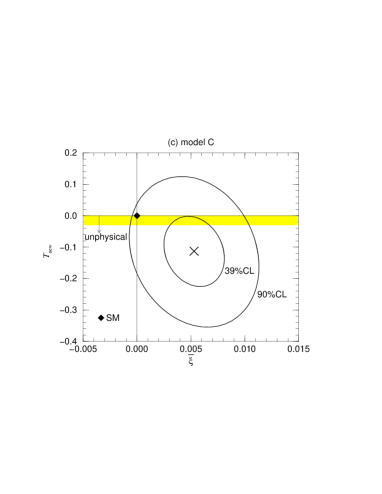
Figure 1: The $\bar{\xi}$ and $T_{\rm new}$ fit to all electroweak data. In all cases $m_{t}$=175.6 $\pm$ 5.5 GeV, $\alpha_{s}(m_{Z_{1}})$ = 0.118 $\pm$ 0.03 and $1/\bar{\alpha}(m^{2}_{Z_{1}})$ = 128.75 $\pm$ 0.09 are taken as the external constraints. Also we assume $S_{\rm new}=U_{\rm new}=0$ and $m_{H}=100$ GeV. The region of $T_{\rm new}<0$ is unphysical in each case. The inner and outer contours correspond to $\Delta\chi^{2}$ = 1 ($\sim$ 39$\%$ CL) and $\Delta\chi^{2}$ = 4.61 ($\sim$ 90$\%$ CL), respectively. The minimum of $\chi^{2}$ is marked by the sign ’$\times$’, whose magnitudes are 21.0, 20.7 and 17.9 for the models A, B and C, respectively. The point $\bar{\xi}=T_{\rm new}=0$ represents the SM result ($\chi^{2}_{\rm min}\sim$ 21.8).

4.2.2 Model B [9]

The five-parameter fit gives

$$\left.\begin{array}[]{cclcl}T_{\rm new}&=&-0.110\;\>+0.154x_{H}&\pm&0.119\\ \bar{\xi}&=&-0.0018+0.0006x_{H}&\pm&0.0023\end{array}\right\}\rho_{\rm corr}=0.38,$$ (4.9c)

$$\chi^{2}_{\rm min}/({\rm d.o.f.})=(20.7+1.3x_{H})/(19).$$ (4.9d)

The result for $x_{H}$ = 0 is shown in Fig. 1b. In the model B, not only $T_{\rm new}$ and $\bar{\xi}$ are consistent with zero but also the $\chi^{2}_{\rm min}$ does not improve from its SM value (4.7). When we impose the condition $T_{\rm new}\geq 0$, the $\chi^{2}_{\rm min}$ takes a minimum value, 21.4, which is almost independent of $x_{H}$ in the range $0.19\!<\!x_{H}\raisebox{1.70717pt}{$<$}\raisebox{-3.69885pt}{$\sim$}0.41$. No noticeable improvement nor worsening of the fit is found from the pull factors listed in Table 2.

4.2.3 Model C [10]

$\begin{array}[]{cc}\leavevmode\psfig{width=199.16928pt}&\leavevmode\psfig{width=199.16928pt}\\ \leavevmode\psfig{width=199.16928pt}&\leavevmode\psfig{width=199.16928pt}\end{array}$

Figure 2: The 95$\%$ CL lower mass limit of the heavier mass eigenstate $Z_{2}$ as a function of the effective mixing parameter $\zeta$ in (2.12).

The five-parameter fit gives

$$\left.\begin{array}[]{cclcl}T_{\rm new}&=&-0.112\;\>+0.143x_{H}&\pm&0.112\\ \bar{\xi}&=&\makebox[9.3894pt]{ }0.0052-0.0001x_{H}&\pm&0.0028\end{array}\right\}\rho_{\rm corr}=-0.18,$$ (4.10c)

$$\chi^{2}_{\rm min}/({\rm d.o.f.})=(17.9+1.1x_{H})/(19).$$ (4.10d)

The result is shown in Fig. 1c for $x_{H}$ = 0 ($m_{H}$ = 100 GeV). In the model C, the positive value of the mixing parameter $\bar{\xi}$ is favored ($\sim 2\sigma$), and $\chi^{2}_{\rm min}$ improves by about three from that of the SM value (4.7). From the pull factors listed in Table 2, we find that the improvement of the fit occurs for two observables, $R_{b}$ and $Q_{W}(^{133}_{55}C_{s})$, as originally arranged in ref. [10]. When we impose the condition $T_{\rm new}\geq 0$, the $\chi^{2}_{\rm min}$ takes a minimum value, 18.6, which is almost independent of $x_{H}$ in the range $0.20\!<\!x_{H}$ $<$$\sim$0.41. The probability of the fit, however, does not improve significantly over that of the SM.

4.3 $Z_{2}$ mass bounds

The above study shows that no significant improvement over the SM is found for the three leptophobic $Z^{\prime}$ models in the latest electroweak data. In this subsection, we obtain the 95$\%$ CL lower mass limit of the heavier mass eigenstate $Z_{2}$. From eq. (2), it is clear that no constraint is found at $\zeta=0$. At a fixed non-zero $\zeta$, the parameter $T_{\rm new}$ and $\bar{\xi}$, which parametrize the effect of the $Z$-$Z^{\prime}$ mixing, can be expressed in terms of the ratio of the physical masses $m^{2}_{Z_{1}}/m^{2}_{Z_{2}}$ for a given value of $g_{E}/g_{Y}$. For each $\zeta$ and $g_{E}/g_{Y}$, we can express the $\chi^{2}$-function in terms of the positive parameter $m^{2}_{Z_{1}}/m^{2}_{Z_{2}}$. We then find the 95$\%$ CL upper bound $r_{95}$ on the ratio $r=m^{2}_{Z_{1}}/m^{2}_{Z_{2}}$ from the condition

$$\int^{\infty}_{r_{95}}dre^{-\frac{\chi^{2}(r)}{2}}=0.95\int^{\infty}_{0}dre^{-\frac{\chi^{2}(r)}{2}}.$$ (4.11)

The 95$\%$ lower mass bound for $Z_{2}$ is then obtained as $m_{Z_{1}}/\sqrt{r_{95}}$. The results are shown in Fig. 2a, b and c for the models A, B and C, respectively. As may be expected from the small mixing formulae (2), the approximate scaling low is found for the $g_{E}/g_{Y}$-dependence of the limit: $m_{Z_{2}}g_{Y}/g_{E}$ is roughly independent of $g_{E}/g_{Y}$. In Fig. 2d, we show the small $\zeta$ region more clearly by using the linear scale for the three models at $g_{E}=g_{Y}$. The $Z^{\prime}$ boson with $m_{Z_{2}}<1$ TeV is allowed by the electroweak data (for $g_{E}=g_{Y}$) only when the effective mixing parameter $\zeta$ (2.12) satisfies the following conditions: $-0.8\!<\!\zeta\!<\!0.7$, $-0.8\!<\!\zeta\!<\!0.8$ and $-0.9\!<\!\zeta\!<\!0.8$ for the models A, B and C, respectively.

Throughout our analysis, we have neglected the effects of the direct exchange of the $Z_{2}$ boson, which is proportional to the mixing angle $\xi$. We find that the 95$\%$ CL lower bounds on $m_{Z_{2}}$ are slightly weakened by taking account of such effects, at most 3 GeV for $|\zeta|$ = 0.05. For larger $|\zeta|$, the effect is negligible because of higher lower mass bound of $m_{Z_{2}}$.

The lower mass limit of $Z_{2}$ also depends on the Higgs boson mass. Because of the condition $T_{\rm new}\geq 0$ (2.11b) and large $m_{H}$ makes the best-fit value of $T_{\rm new}$ large, the $Z_{2}$ mass bound tends to weak as the Higgs boson mass increases. At $|\zeta|$ = 1, the mass bounds for $m_{H}$ = 80 (150) GeV are $4\%$ ($8\%$) severer (weaker) than that for $m_{H}$ = 100 GeV.

5 Summary

In this paper, we have investigated the constraints on the three leptophobic $Z^{\prime}$ models from the latest electroweak data. The $Z^{\prime}$ boson in the model A [8] is essentially $Z_{\eta}$ of the string-inspired $E_{6}$ model with large kinetic mixing, that in the model B [9] couples only to the decouplet of the flipped SU(5)$\times$U(1) GUT. In the model C [10] the $Z^{\prime}$ couplings to quarks are determined by refering to the electroweak data of 1995. In our parametrization, the $Z$-$Z^{\prime}$ mixing effects are parametrized in terms of the effective mass mixing parameter $\bar{\xi}$ and the non-SM contribution $T_{\rm new}$ to the electroweak $T$ parameter due to the mass shift $\Delta m^{2}=m^{2}_{Z_{1}}-m^{2}_{Z}$. Since the mass shift $\Delta m^{2}$ is negative, $T_{\rm new}$ is positive definite. Compact parametrizations of the predictions of the SM and the three leptophobic $Z^{\prime}$ models are given for all the electroweak observables. From the fit to the latest electroweak data, we find that none of the three models gives a significantly improved fit over the SM. The improvement in $\chi^{2}_{\rm min}$ is found to be at most three (for the model C) while each model has two additional parameters, $\bar{\xi}$ and $T_{\rm new}$.

Finally, we have obtained the 95$\%$ CL lower mass limit of the heavier mass eigenstate $Z_{2}$. When the mixing parameter $\zeta$ (2.12) is large, $|\zeta|>1$, the lower mass bound exceeds 1 TeV for all the models. The leptophobic $Z^{\prime}$ boson lighter than 1 TeV is allowed only in the range $-0.8\!<\!\zeta\!<\!0.7$, $-0.8\!<\!\zeta\!<\!0.8$ and $-0.9\!<\!\zeta\!<\!0.8$ for the models A, B and C respectively, for $g_{E}=g_{Y}$ and $m_{H}$ = 100 GeV.

References

- [1] The LEP Collaborations ALEPH, DELPHI, L3, OPAL, the LEP Electroweak Working Group and the SLD Heavy Flavor Group, CERN-PPE/97-154.
- [2] J. Hewett and T. Rizzo, Phys. Rep. 183 (1989) 193.
- [3] P. Langacker and M. Luo, Phys. Rev. D45 (1992) 278.
- [4] G.C. Cho, K. Hagiwara, and S. Matsumoto, Eur. Phys. J. C5(1998)155.
-
[5]
T. Gehrmann and W.J. Stirling, Phys. Lett. B381 (1996) 221;
V. Barger, Kingman Cheung, and P. Langacker, Phys. Lett. B381 (1996) 226;
H. Georgi and S.L. Glashow, Phys. Lett. B387 (1996) 341;
-
[6]
G. Altarelli, N. Di Bartolomeo, F. Feruglio, R.Gatto,
and M.L. Mangano, Phys. Lett. B375 (1996) 292;
P. Chiappetta, J.Layssac, F.M. Renard, and C. Verzegnassi, Phys. Rev. D54 (1996) 789. -
[7]
A.E. Faraggi and M. Masip, Phys. Lett. B388 (1996) 524;
M. Cvetič and P. Langacker, Mod. Phys. Lett. A11 (1996) 1247. - [8] K.S. Babu, C. Kolda, and J. March-Russell, Phys. Rev. D54 (1996) 4635.
- [9] J.L. Lopez and D.V. Nanopoulos, Phys. Rev. D55 (1997) 397.
- [10] K. Agashe, M. Graesser, I. Hinchliffe, and M. Suzuki, Phys. Lett. B385 (1996) 218.
-
[11]
L3 Collaboration, O. Adriani et al., Phys. Lett. B306 (1993) 187;
ALEPH Collaboration, D. Buskulic et al., Z. Phys. C62 (1994) 539. - [12] CDF collaboration, F. Abe et al., Phys. Rev. Lett. 79 (1997) 2192.
- [13] K. Hagiwara, D. Haidt, C.S. Kim, and S. Matsumoto, Z. Phys. C64 (1994) 559; C68 (1995) 352 (E).
- [14] M.E. Peskin and T. Takeuchi, Phys. Rev. Lett. 65 (1990) 964; Phys. Rev. D46 (1992) 381.
- [15] B. Holdom, Phys. Lett. B166 (1986) 196.
- [16] CDF collaboration, J. Lys, talk at ICHEP96, in Proc. of ICHEP96, (ed) Z. Ajduk and A. K. Wroblewski, World Scientific, (1997); D0 Collaboration, S. Protopopescu, talk at ICHEP96, in the proceedings.
- [17] B. Holdom, Phys. Lett. B259 (1991) 329.
- [18] K.S. Babu, C. Kolda, and J.March-Russell, Phys. Rev. D57 (1998) 6788.
- [19] Particle Data Group, R.M. Barnett et al., Phys. Rev. D54 (1996) 1.
- [20] S. Eidelman and F. Jegerlehner, Z. Phys. C67 (1995) 585.
- [21] K. Hagiwara, D. Haidt, and S. Matsumoto, Eur. Phys. J. C2 (1998) 95.
- [22] J.E. Kim, P. Langacker, M. Levine, and H.H. Williams, Rev. Mod. Phys. 53 (1981) 211.
- [23] C.Y. Prescott et al., Phys. Lett. B84 (1979) 524.
- [24] A. Argento et al., Phys. Lett. B120 (1983) 245.
- [25] P.A. Souder, in Precision tests of the standard electroweak model, (ed) P. Langacker, World Scientific (1995), 599.
- [26] P.A. Souder et al., Phys. Rev. Lett. 65 (1990) 694.
- [27] W. Heil et al., Nucl. Phys. B327 (1989) 1.
- [28] W.J. Marciano and A. Sirlin, Phys. Rev. D27 (1983) 552.
- [29] M.C. Noecker, B.P. Masterson, and C.E. Wieman, Phys. Rev. Lett. 61 (1988) 310.
- [30] C.S. Wood et al., Science 275 (1997) 1759.
- [31] G.L. Fogli and D. Haidt, Z. Phys. C40 (1988) 379.
- [32] K. McFarland et al., Eur. Phys. J. C1 (1998) 509.
- [33] P. Janot, talk at International Europhysics Conference on High Energy Physics (EPS97), Jerusalem, 1997.
- [34] G.L. Kane, C. Kolda, and J.D. Wells, Phys. Rev. Lett. 70 (1993) 2686.