Hadronic Axion Model in Gauge-Mediated Supersymmetry Breaking

Abstract

A simple hadronic axion model is proposed in the framework of gauge-mediated supersymmetry breaking. Dynamics of Peccei-Quinn symmetry breaking is governed by supersymmetry breaking effects and the Peccei-Quinn breaking scale $f_{PQ}$ is inversely proportional to the gravitino mass. The gravitino mass range which corresponds to the axion window $f_{PQ}\simeq 10^{9}$ GeV – $10^{13}$ GeV lies in the region predicted by gauge-mediated supersymmetry breaking models. The model is also shown to be cosmologically viable.

The Peccei-Quinn (PQ) mechanism [1] is so far the most attractive framework to solve the strong CP problem. The essential ingredient of this mechanism is a global U(1$)_{PQ}$ symmetry which is, apart from breaking by the QCD anomaly, spontaneously broken. The resulting Goldstone mode (axion) acquires a small mass due to the QCD anomaly. When one considers the PQ mechanism in the context of supersymmetry (SUSY), there appears a non-compact flat direction associated with the U(1)_PQ Goldstone mode. The degeneracy of the vacua is resolved by effects of SUSY breakdown. The properties of the PQ mechanism should therefore depend on details of the SUSY breakdown. In this paper, we would like to propose a simple model which works as the PQ mechanism in the framework of gauge-mediated SUSY breaking, while most of the previous study has been done in gravity-mediated SUSY breaking.

We shall first describe our proposal. We consider a KSVZ axion model[2] (so called a hadronic axion model). A gauge-singlet Peccei-Quinn (PQ) multiplet $X$ and also new PQ quarks $Q_{P}$ and $\overline{Q}_{P}$ (3 and ${\bf 3}^{\ast}$ in SU(3)_C) are introduced. Their U(1)_PQ charges are assigned as ${\cal Q}[X]=+1$, ${\cal Q}[Q_{P}]=-1/2$ and ${\cal Q}[\overline{Q}_{P}]=-1/2$. The superpotential of the PQ sector takes the following simple form:

$$W_{PQ}=\lambda_{P}XQ_{P}\overline{Q}_{P},$$ (1)

where $\lambda_{P}$ is a coupling constant. Note that no mass parameter is introduced in the superpotential. Eq. (1) gives the potential of the scalar fields in the SUSY limit as

$$V(X,\widetilde{Q_{1}},\widetilde{Q_{2}}) = \lambda_{P}^{2}\left[\left|\widetilde{Q_{2}}^{\dagger}\widetilde{Q_{1}}\right|^{2}+\left|X\right|^{2}\left(\left|\widetilde{Q_{1}}\right|^{2}+\left|\widetilde{Q_{2}}\right|^{2}\right)\right]$$ (2)

$$+ \frac{g_{s}^{2}}{2}\left[\widetilde{Q_{1}}^{\dagger}T^{a}\widetilde{Q_{1}}-\widetilde{Q_{2}}^{\dagger}T^{a}\widetilde{Q_{2}}\right]^{2},$$ (3)

where $g_{s}$ and $T^{a}$ denote the QCD coupling and generators. $X$ is the PQ scalar field, and $\widetilde{Q_{1}}$ and $\widetilde{Q_{2}}$ are PQ squarks.

From the potential (3) one finds a flat direction along the $X$ axis with $\widetilde{Q_{1}}=\widetilde{Q_{2}}=0$. This comes from the fact that the superpotential (1) has an extended U(1$)_{PQ}$ symmetry [3]. Because it is a holomorphic function, the superpotential which possesses the conventional U(1$)_{PQ}$ symmetry is also invariant under the complex form of the U(1) transformation (i.e. the dilatational transformation). This extended symmetry results in the flat direction of the scalar potential (3) when the SUSY is an exact symmetry. However, the flat direction is lifted through SUSY breaking effects.

In gauge-mediated SUSY breaking theories (for a review see ref. [4]), the standard model (SM) gauge interaction transmits SUSY breaking effects from a messenger sector to ordinary squarks and sleptons at two-loop level. At the same level the PQ squarks $\widetilde{Q_{1}}$ and $\widetilde{Q_{2}}$ also feel SUSY breaking through the QCD interaction, whereas the PQ scalar $X$ is a gauge singlet and thus feels SUSY breaking through the Yukawa interaction (1) only after the PQ squarks receive SUSY breaking masses. Then the induced potential for $X$ is so suppressed that we should not neglect the SUSY breaking effect mediated by gravity. Indeed as we will see shortly, the balance between the gravity-mediated effect and the gauge-mediated effect determines the minimum of the $X$ field. In the following, we estimate the potential of the flat direction induced by the SUSY breaking effects by considering the both mediation mechanisms.

Effects of SUSY breaking communicated by the gravity are expected to induce the soft SUSY breaking mass to the PQ scalar field comparable to the gravitino mass $m_{3/2}$ which is much smaller than the electroweak scale in the gauge-mediated SUSY breaking models ($m_{3/2}\sim 10^{-2}$ keV–1 GeV). Then through the gravity-mediation the flat direction obtains the potential $V_{H}$ as

$$V_{H}(X)\simeq\frac{1}{2}\xi^{2}m_{3/2}^{2}\left|X\right|^{2},$$ (4)

where $\xi^{2}$ is a dimension-less parameter of the order one, which we assume to be positive. We have neglected higher order terms because they are suppressed by the gravitational scale.

On the other hand, effects of SUSY breaking through the gauge-mediation mechanism also generate a potential $V_{G}$ to the PQ $X$ field. In most models of the gauge-mediation[5, 6] SUSY is broken by some non-perturbative dynamics in a “hidden” sector and its effects are fed down to a messenger sector. In the messenger sector, a gauge-singlet chiral multiplet $Z$ is supposed to have a $A$-component vacuum expectation value (vev) $\left<Z\right>$ and a $F$-component vev $\left<F_{Z}\right>$ as well. This singlet couples to messenger quark multiplets $q_{M}$ and $\overline{q}_{M}$ which are $\bf 3$ and $\bf 3^{\ast}$ in SU(3)_C, in the superpotential

$$W_{M}=\lambda_{M}~{}Z~{}q_{M}\overline{q}_{M}$$ (5)

with $\lambda_{M}$ a dimension-less coupling. The superpotential (5) induces a mass of the messenger quark $\Psi_{q}$ as $m_{\Psi_{q}}=M$ and the messenger squarks $\widetilde{q}_{\pm}$ obtain masses squared as $m_{\widetilde{q}_{\pm}}^{2}=M(M\pm\Lambda)$. Here we define $M$ and $\Lambda$ by

$$\lambda_{M}\left<Z\right> \equiv M,$$ (6)

$$\lambda_{M}\left<F_{Z}\right> \equiv M\Lambda.$$ (7)

Then the SUSY is broken in the messenger sector and its effects are mediated to the ordinary sector through the SM gauge interaction by integrating out the heavy messenger fields.

The PQ squarks $\widetilde{Q_{1}}$ and $\widetilde{Q_{2}}$, similar to the squarks in the standard model sector, obtain soft SUSY breaking masses from two-loop diagrams of the messenger multiplets, gluon and gluino. Then the SUSY breaking effects are transmitted to the PQ $X$ field by “one-loop” diagrams of $\widetilde{Q_{1}}$ and $\widetilde{Q_{2}}$.

We made an explicit calculation of the effective potential for the PQ scalar $X$, $V_{G}(X)$, along the flat direction induced by the above gauge-mediation mechanism. Here we present only the final result and the details are found in Appendix. To estimate the minimum of the potential, the derivative of the potential with respect to $X^{2}$ is sufficient rather than $V_{G}$ itself. The result is given by

$$\frac{\partial V_{G}(X^{2})}{\partial X^{2}} = ~{}-~{}\frac{8\alpha_{s}^{2}}{(4\pi)^{4}}\frac{M^{2}\Lambda^{2}}{X^{2}}\log^{2}\left(\frac{\lambda_{P}^{2}X^{2}}{M^{2}}\right).$$ (8)

Here we have presented the asymptotic form which is valid only for $X\gg M$. This is because for $X\stackrel{{\scriptstyle<}}{{{}_{\sim}}}M$, the gauge-mediation generates a sizable negative curvature for the $X$ field in a standard manner, which shifts the vev of the field far away from the origin. Thus we expect that the minimum of $X$ is much larger than $M$. This is a good news for phenomenology because there is some chance that the resulting PQ scale falls into the cosmological axion window, which is indeed the case, as we will see shortly.

The potential along the flat direction $X$ generated by the two SUSY breaking effects is thus given by

$$V_{eff}(X)=V_{H}(X)+V_{G}(X).$$ (9)

Using eqs. (4) and (8) we can estimate the vev of the PQ scalar field, $X_{c}\equiv\left<X\right>\gg M$, by looking into the minimization condition of the potential

$$0=\frac{\partial V_{H}(X)}{\partial X}+\frac{\partial V_{G}(X)}{\partial X},$$ (10)

which yields

$$X_{c} \simeq \frac{1}{\xi\pi}\left(\frac{\alpha_{s}}{4\pi}\right)\frac{M\Lambda}{m_{3/2}}\log\left(\frac{\lambda_{P}^{2}X_{c}^{2}}{M^{2}}\right).$$ (11)

The PQ scalar field thus develops a vev, and the U(1)_PQ symmetry is spontaneously broken and the PQ scale is given as $f_{PQ}=X_{c}$. We would like to emphasize that in the present axion model the PQ scale is determined by only the SUSY breaking scales without introducing any other mass scales. We present the numerical values of the PQ scale in Fig.1. If we take the parameters of the messenger sector as $\Lambda$ = 40 TeV and $M$ = 50 TeV the PQ scale is approximately given by

$$f_{PQ}=X_{c}\simeq\frac{10^{11}~{}\mbox{GeV}}{\xi}\left(\frac{1~{}\mbox{MeV}}{m_{3/2}}\right),$$ (12)

for $\lambda_{P}$ = 1. Therefore this model provides a simple description of the PQ mechanism in the gauge-mediated SUSY breaking theories. Note that in the simplest structure of the messenger sector, our choice of $\Lambda$ yields the right-handed slepton mass of about 90 GeV. On the other hand, the choice of $M$ is somewhat arbitrary, though $M$ must be larger than $\Lambda$ to avoid a negative mass squared for the messenger squark, and thus one should regard (12) as the lower bound of the PQ scale for a given gravitino mass. One should keep this point in mind, though in the following we take $M=50$ TeV for our representative value.

In SUSY theories, the axion forms a chiral multiplet. In addition to the axion, which can be chosen as the imaginary part of the complex scalar $X$, the multiplet contains a saxion $s$, the real part of $X$, and an axino $\tilde{a}$, the fermionic component of the multiplet. Parameterizing $X$ = $(s/\sqrt{2}+X_{c})\exp\left(ia/(\sqrt{2}X_{c})\right)$ the mass of the saxion is easily evaluated as

$$m_{s} = \xi m_{3/2}.$$ (13)

Thus the saxion acquires a mass comparable to the gravitino, while the axion $a$ gets a mass from the QCD effect as $m_{a}\simeq f_{\pi}m_{\pi}/f_{PQ}$.

We shall next consider cosmology of this axion model to see whether or not it is cosmologically viable. The axion relic abundance from the misalignment is given as [8, 9]

$$\Omega_{a}h^{2}\sim 0.2\theta^{2}\left(\frac{f_{PQ}}{10^{12}\mbox{GeV}}\right)^{1.18}$$ (14)

with $\theta$ being the initial misalignment angle ($|\theta|<\pi$) and $h$ the Hubble constant in units of 100 km/sec./Mpc. In ignorance of the misalignment angle and with theoretical uncertainty of order unity in the evaluation of Eq. (14), we could say that the axion may be able to constitute the dominant component of the dark matter of the universe if

$$10^{11}\mbox{GeV}\stackrel{{\scriptstyle<}}{{{}_{\sim}}}f_{PQ}\stackrel{{\scriptstyle<}}{{{}_{\sim}}}10^{13}\mbox{GeV}.$$ (15)

The same argument implies an upper bound of the axion scale $f_{PQ}\stackrel{{\scriptstyle<}}{{{}_{\sim}}}10^{13}\mbox{GeV}$. On the other hand, the cooling of the SN 1987A puts a lower bound of about $10^{9}$ GeV [10]. Thus the following range

$$10^{9}\mbox{GeV}\stackrel{{\scriptstyle<}}{{{}_{\sim}}}f_{PQ}\stackrel{{\scriptstyle<}}{{{}_{\sim}}}10^{13}\mbox{GeV}$$ (16)

is regarded as the allowed region of the PQ scale. With eq. (12), this in turn identifies the allowed range of the gravitino mass in this scenario:

$$100\mbox{MeV}\stackrel{{\scriptstyle>}}{{{}_{\sim}}}\xi m_{3/2}\stackrel{{\scriptstyle>}}{{{}_{\sim}}}10\mbox{keV}.$$ (17)

Remarkably the gauge-mediated SUSY breaking naturally gives the gravitino mass in this range. The region of $m_{3/2}$ is somewhat shifted if we take a different value of $M$, but still the gravitino mass range fits with the gauge-mediation mechanism as far as $M\stackrel{{\scriptstyle<}}{{{}_{\sim}}}10^{9}$ GeV with $\Lambda\simeq 40$ GeV fixed. On the other hand, this model does not give the possible hadronic axion window $f_{PQ}\sim 10^{6}$ GeV.

Let us next consider cosmology of the saxion. It dominantly decays to two axions through the interaction given by

$$\partial_{\mu}X^{\dagger}\partial^{\mu}X=\frac{1}{2}\partial_{\mu}s\partial^{\mu}s+\frac{1}{2}\partial_{\mu}a\partial^{\mu}a+\frac{1}{\sqrt{2}{X_{c}}}s\partial_{\mu}a\partial^{\mu}a+\cdots.$$ (18)

The decay width is estimated as

$$\Gamma(s\rightarrow aa)=\frac{1}{64\pi}\frac{m_{s}^{3}}{f_{PQ}^{2}},$$ (19)

from which we find the lifetime

$$\tau_{s}\simeq 1.3\times 10^{9}\mbox{sec}\left(\frac{1\mbox{MeV}}{m_{s}}\right)^{5}\simeq\frac{1.3\times 10^{9}\mbox{sec}}{\xi^{5}}\left(\frac{1\mbox{MeV}}{m_{3/2}}\right)^{5}.$$ (20)

It varies widely from $10^{-1}$–$10^{19}$ sec. for the gravitino mass range (17). With this long lifetime, we have to see its cosmological consequences carefully.

To go further, we need to estimate the saxion abundance. The saxion decouples from the thermal bath at the temperature about [11]

$$T_{dec}\simeq 10^{9}\mbox{GeV}\left(\frac{f_{PQ}}{10^{11}\mbox{GeV}}\right)^{2}.$$ (21)

If the decoupling temperature were lower than the reheat temperature after the inflation, then the yield of the saxion (defined by the number density of the saxion divided by the entropy density) would be $Y_{s}\sim 10^{-3}$. However the gravitino problem in the GMSB suggests relatively low $T_{R}$. For the gravitino mass range considered here, the closure limit of the gravitino gives [12, 13]

$$T_{R}\stackrel{{\scriptstyle<}}{{{}_{\sim}}}10^{6}\mbox{GeV}\left(\frac{m_{\tilde{g}}}{300\mbox{GeV}}\right)^{-2}\left(\frac{m_{3/2}}{1\mbox{MeV}}\right),$$ (22)

where $m_{\tilde{g}}$ denotes the gluino mass. So the decoupling temperature is higher than the reheat temperature, and saxions are not thermalized. However saxions are produced by scattering e.g. $q\bar{q}\rightarrow sg$ in the thermal bath, with the yield [14, 15]

$$Y_{s}\sim 10^{-3}\left(\frac{T_{R}}{T_{dec}}\right)\sim 10^{-6}\left(\frac{f_{PQ}}{10^{11}\mbox{GeV}}\right)^{-2}\left(\frac{T_{R}}{10^{6}\mbox{GeV}}\right),$$ (23)

and thus

$$m_{s}Y_{s}\sim 10^{-9}\mbox{GeV}\left(\frac{m_{s}}{1\mbox{MeV}}\right)\left(\frac{f_{PQ}}{10^{11}\mbox{GeV}}\right)^{-2}\left(\frac{T_{R}}{10^{6}\mbox{GeV}}\right).$$ (24)

The saxion is also produced as its coherent oscillation. An inspection shows that with the low reheat temperature given by (22) the saxion starts to oscillate while the inflaton obeys coherent oscillation (before the reheating process is completed). We estimate the abundance to be

$$m_{s}Y_{s}\sim\frac{1}{8}\left(\frac{s_{i}}{M_{G}}\right)^{2}T_{R}\simeq 10^{-10}\mbox{GeV}\left(\frac{s_{i}}{f_{PQ}}\right)^{2}\left(\frac{f_{PQ}}{10^{11}\mbox{GeV}}\right)^{2}\left(\frac{T_{R}}{10^{6}\mbox{GeV}}\right),$$ (25)

where $s_{i}$ is the initial amplitude of the saxion oscillation, which is expected to be of order $f_{PQ}$.

In the above, we have assumed that the vacuum expectation value of the field $X$ is displaced from the origin during the reheating process: otherwise thermal effects would generate a positive mass for $X$, trapping the $X$ field at the origin until the universe cools down below the weak scale. In this case, the above estimate is no longer valid, and we expect that the relic abundance of the saxion will be much larger, which may be problematic. The displacement of the field $X$ may be achieved by fluctuations of the field during the de Sitter expansion in the inflationary phase. In the following, we use the maximum of (24) and (25) as the saxion abundance. It remains constant as time goes on as far as no entropy production occurs. Note that the abundance is proportional to the reheat temperature.

Let us next consider bounds on the abundance of the saxions and the axions produced by the saxion decay. Existence of exotic particles around the cosmic temperature $T\sim 1$ MeV may accelerate the expansion of the universe and increase the neutron-to-proton number ratio at the decoupling, resulting in too much ⁴He abundance. Roughly speaking, the abundance of such exotic particles should not exceed that of one neutrino species, namely

$$m_{s}Y_{s}\stackrel{{\scriptstyle<}}{{{}_{\sim}}}10^{-4}\mbox{GeV}.$$ (26)

This is not significant.

The energy densities of the saxions and the produced axions may alter the evolution of the universe at much later time, e.g. the age of the universe and the time of matter-radiation equality. However, if the abundance of the produced saxions does not exceed the critical density of the universe (divided by the present entropy density), namely

$$m_{s}Y_{s}\stackrel{{\scriptstyle<}}{{{}_{\sim}}}3.6\times 10^{-9}h^{2}\mbox{GeV},$$ (27)

then the standard cosmology is not affected. We find that the condition (27) is easily satisfied for a certain range of the reheat temperature.

The next bounds we consider are those from rare decay modes of the saxion. Since the saxion is light, it does not decay to gluons. On the other hand, it generally decays to photons. The branching ratio of the radiative decay of the saxion, $B$, is typically of the order $(\alpha/4\pi)^{2}\sim 10^{-6}$. For $\tau_{s}\stackrel{{\scriptstyle<}}{{{}_{\sim}}}10^{6}$ sec. the constraint on the radiative decay comes from the photodissociation of the light elements (for a recent analysis, see ref. [16]). For $\tau_{s}\stackrel{{\scriptstyle>}}{{{}_{\sim}}}10^{6}$ sec., the non-observation of the distortion of the cosmic microwave background gives a tighter bound on the abundance of the produced photons: $B\times m_{s}Y_{s}\stackrel{{\scriptstyle<}}{{{}_{\sim}}}2\times 10^{-13}$ GeV $(10^{10}$sec.$/\tau_{s})^{1/2}$ for $\tau_{s}\sim 10^{6}$–$10^{10}$ sec. and $B\times m_{s}Y_{s}\stackrel{{\scriptstyle<}}{{{}_{\sim}}}2\times 10^{-14}$ GeV $(10^{12}$sec.$/\tau_{s})^{2/3}(\Omega_{0}h^{2})^{-1/3}$ for $\tau_{s}\sim 10^{10}$–$10^{12}$ sec. [17]. Comparing the above bounds with the predicted abundance (24) or (25) multiplied by the very small branching ratio $B$, we find that the saxion abundance easily survives these bounds even with relatively a high reheat temperature close to the upper bound allowed by the gravitino problem. On the other hand, when the saxion decays after the recombination ($\tau_{s}\stackrel{{\scriptstyle>}}{{{}_{\sim}}}10^{12}$ GeV), a stringent constraint comes from the diffuse X-ray backgrounds. The strongest one is $B\times m_{s}Y_{s}\stackrel{{\scriptstyle<}}{{{}_{\sim}}}10^{-17}$ GeV for $\tau_{s}\sim 10^{17}$ sec. [18]. We find that this severe constraint is fulfilled if the reheat temperature is lower than 10 GeV so that the saxion abundance is highly suppressed.

Summarizing the above arguments, we conclude that our model can be viable in view of the saxion cosmology.

It is noteworthy to mention that the case where the saxion abundance exceeds (27) is not immediately ruled out. Rather the saxion may modify the universe’s evolution in an interesting way. Probably the most interesting case [19, 14] is that the saxion energy density once dominates the universe before it decays to axions. Then the produced axions behave as an extra contribution to the radiation when we consider the cosmological developments, which delay the epoch of the matter-radiation equality. In this case, the saxion may play a role of the late decaying particle which will reconcile the standard cold dark matter (CDM) dominated universe for $h>0.5$ with the large scale structure formation, if the following is fulfilled [14]

$$\left(\frac{\tau_{s}}{1\mbox{sec}}\right)\left(\frac{m_{s}Y_{s}}{1\mbox{MeV}}\right)^{2}\simeq 0.55((h/0.2)^{2}-1)^{3/2}.$$ (28)

In particular, our model provides a concrete realization of ref. [15], where a hypothetically light saxion is proposed to play this role.

Finally we will look into the axino, the fermionic superpartner of the axion. Radiative corrections with the messenger fields give an axino mass. In our case, the contribution appears at the three-loop level, and it is $\sim m_{3/2}^{2}/\Lambda\ll m_{3/2}$. The axino mass is also induced by supergravity effects and in general it becomes of the order of the gravitino mass [20, 21, 22]. An inspection shows that, however, in this simple model, the leading contribution of the order $m_{3/2}$ is cancelled, and the non-vanishing contribution is $\sim(f_{PQ}^{2}/M_{G}^{2})m_{3/2}\ll m_{3/2}$. Thus the axino is much lighter than the gravitino. The axinos are produced by scattering after the inflationary epoch and we expect that the yield of the axinos is more or less the same as that of the saxions (23). In our case, since the axino is much lighter than the saxion, the axino energy density is always smaller than the saxion’s one and thus it is harmless. Another possible worry is that the gravitino decay to an axino and an axion is kinematically allowed. However, with the mass range of the gravitino considered here, the lifetime is much longer than the age of the universe, hence the gravitino is essentially stable. Thus the light axino appeared in this model does not alter the argument above and it is cosmologically harmless.

To conclude, we proposed the hadronic axion model in the gauge-mediated SUSY breaking theories. The model gives a simple description on the PQ symmetry breaking mechanism which is solely governed by the SUSY breaking physics. It should be noted that the PQ scale is inversely scaled to the gravitino mass and the resulting PQ scale naturally falls into the axion window, for the gravitino mass range favored by the gauge-mediation. Moreover the axion becomes a dark matter candidate for $m_{3/2}\sim 10$ keV–1 MeV. Next we investigated cosmological implications of the other particles in the axion supermultiplet, namely the saxion and the axino, and showed that our model is cosmologically acceptable with sufficiently low reheat temperature which is suggested by the gravitino problem. Finally we pointed out that the saxion in this model may play a role of the late-decaying particle, causing the delay of the matter-radiation equality, and consequently reconciling the standard CDM with the structure formations of the universe. Details of this issue will be discussed elsewhere [23].

Effective Potential for PQ Scalar Field $X$

Here we derive the potential for the PQ scalar field $X$ induced by the SUSY breaking effects through gauge-mediation mechanism. We calculate an effective potential for $X_{c}$, the classical value of the $X$ field. As the ordinary squarks, the PQ squarks receives the SUSY breaking effects from the messenger sector by the QCD interaction at two-loop level. Then the effects are transmitted to $X$ by the Yukawa interaction (1) at three-loop order. The Feynmann diagrams for the vacuum energy which should be estimated are shown in Figs. 2, 4 and 5. In our calculation we expand it in terms of the $M\Lambda$ and estimate the leading term of ${\cal O}((M\Lambda)^{2})$, i.e., the leading term with $F$-vev of the messenger multiplet. From the Yukawa interaction (1) the PQ quark and squark acquire a mass $M_{Q}=\lambda_{P}X_{c}$.

First, we estimate the vacuum energy induced by the D-term scalar potential which diagram is shown in Fig. 2. This diagram gives

$$iV_{D} = 2\times 2g_{s}^{4}\int\frac{d^{4}k}{(2\pi)^{4}}\int\frac{d^{4}p}{(2\pi)^{4}}\int\frac{d^{4}q}{(2\pi)^{4}}$$ (30)

$$\times\left[\frac{1}{[k^{2}-m_{\widetilde{q}_{+}}^{2}][(k+p)^{2}-m_{\widetilde{q}_{-}}^{2}]}\right]\left[\frac{1}{[q^{2}-M_{Q}^{2}][(q+p)^{2}-M_{Q}^{2}]}\right],$$

where the messenger squark masses are $m_{\widetilde{q}_{\pm}}$ =$M(M\pm\Lambda)$. Then we expand the RHS in terms of $(M\Lambda)$ as

$$iV_{D} = 4g_{s}^{4}\int\frac{d^{4}k}{(2\pi)^{4}}\int\frac{d^{4}p}{(2\pi)^{4}}\int\frac{d^{4}q}{(2\pi)^{4}}\int_{0}^{1}dx\int_{0}^{1}dy\frac{1}{\left[q^{2}+y(1-y)p^{2}-M_{Q}^{2}\right]^{2}}$$ (32)

$$\times\left[\frac{1}{\left[k^{2}+x(1-x)p^{2}-M^{2}\right]^{2}}+\frac{3(1-2x)^{2}(M\Lambda)^{2}}{\left[k^{2}+x(1-x)p^{2}-M^{2}\right]^{4}}+\cdots\right],$$

where the ${\cal O}(M\Lambda)$ term vanishes on making the integration on $x$. Since what we are interested in are the SUSY breaking effects at the first non-vanishing order, we pick up only the ${\cal O}((M\Lambda)^{2})$ term. Thus the effective potential from the D-term interaction is estimated as

$$iV_{D} = g_{s}^{4}\int\frac{d^{4}k}{(2\pi)^{4}}\int\frac{d^{4}p}{(2\pi)^{4}}\int\frac{d^{4}q}{(2\pi)^{4}}\int_{0}^{1}dx\int_{0}^{1}dy$$ (34)

$$\times\frac{12(1-2x)^{2}(M\Lambda)^{2}}{\left[q^{2}+y(1-y)p^{2}-M_{Q}^{2}\right]^{2}\left[k^{2}+x(1-x)p^{2}-M^{2}\right]^{4}}.$$

Next, we turn to the vacuum energy with the gluon fields. We first calculate the one-loop correction to the vacuum polarization from the messenger multiplets, (see Fig.3.) and then estimate the vacuum energy shown in Fig.4. Up to the ${\cal O}((M\Lambda)^{4})$, the result is given by

$$iV_{g} = g_{s}^{4}\int\frac{d^{4}k}{(2\pi)^{4}}\int\frac{d^{4}p}{(2\pi)^{4}}\int\frac{d^{4}q}{(2\pi)^{4}}\int_{0}^{1}dx\int_{0}^{1}dy$$ (36)

$$\times\frac{36(1-2x)^{2}(M\Lambda)^{2}}{\left[q^{2}+y(1-y)p^{2}-M_{Q}^{2}\right]^{2}\left[k^{2}+x(1-x)p^{2}-M^{2}\right]^{4}}.$$

Finally, the vacuum energy induced by the gluino (see Fig.5.) is estimated as

$$iV_{\widetilde{g}} = -g_{s}^{4}\int\frac{d^{4}k}{(2\pi)^{4}}\int\frac{d^{4}p}{(2\pi)^{4}}\int\frac{d^{4}q}{(2\pi)^{4}}\int_{0}^{1}dx\int_{0}^{1}dy$$ (38)

$$\times\frac{192(1-y)(1-x)^{3}(M\Lambda)^{2}}{\left[q^{2}+y(1-y)p^{2}-M_{Q}^{2}\right]^{2}\left[k^{2}+x(1-x)p^{2}-M^{2}\right]^{4}}.$$

Therefore summing up eqs. (34), (36) and (38), we obtain the effective potential $V_{G}$ at the order $(M\Lambda)^{2}$ as

$$V_{G}(M_{Q}^{2}) = ig_{s}^{4}\left(M\Lambda\right)^{2}\int\frac{d^{4}k}{(2\pi)^{4}}\int\frac{d^{4}p}{(2\pi)^{4}}\int\frac{d^{4}q}{(2\pi)^{4}}\int_{0}^{1}dx\int_{0}^{1}dy$$ (40)

$$\times\frac{48x(1-x)}{\left[q^{2}+y(1-y)p^{2}-M_{Q}^{2}\right]^{2}\left[k^{2}+x(1-x)p^{2}-M^{2}\right]^{4}},$$

and by making a Wick rotation it leads to

$$V_{G}(M_{Q}^{2}) = \frac{48g_{s}^{4}}{(4\pi)^{6}}\left(M\Lambda\right)^{2}\int dk\int dp\int dq\int_{0}^{1}dx\int_{0}^{1}dy$$ (42)

$$\times\frac{x(1-x)kpq}{\left[q+y(1-y)p+M_{Q}^{2}\right]^{2}\left[k+x(1-x)p+M^{2}\right]^{4}}.$$

Instead of the effective potential itself, it is more convenient to calculate its derivative. We find

$$\frac{\partial V_{G}(M_{Q}^{2})}{\partial M_{Q}^{2}} = -\frac{96g_{s}^{4}}{(4\pi)^{6}}\left(M\Lambda\right)^{2}\int dk\int dp\int dq\int_{0}^{1}dx\int_{0}^{1}dy$$ (44)

$$\times\frac{x(1-x)kpq}{\left[q+y(1-y)p+M_{Q}^{2}\right]^{3}\left[k+x(1-x)p+M^{2}\right]^{4}}.$$

Now the momentum integrations are straight forward.

$$\frac{\partial V_{G}(M_{Q}^{2})}{\partial M_{Q}^{2}} = -\frac{8g_{s}^{2}}{(4\pi)^{6}}\frac{\left(M\Lambda\right)^{2}}{M_{Q}^{2}}\int_{0}^{1}dx\int_{0}^{1}dy$$ (46)

$$\times\frac{\frac{1}{z^{2}}-x(1-x)+x(1-x)\ln[z^{2}x(1-x)]}{\left[\frac{1}{z^{2}}-x(1-x)\right]^{2}},$$

where $z^{2}=\frac{M_{Q}^{2}}{M^{2}y(1-y)}$. We can perform the $x$ integration analytically. (See ref.[13].) Instead here we give an approximate expression valid for $z^{2}\gg 4$

$$\frac{\partial V_{G}(M_{Q}^{2})}{\partial M_{Q}^{2}} \simeq -\frac{8g_{s}^{4}}{(4\pi)^{6}}\frac{\left(M\Lambda\right)^{2}}{M_{Q}^{2}}\int_{0}^{1}dy\ln^{2}\left[\frac{M_{Q}^{2}}{M^{2}y(1-y)}\right]$$ (47)

$$\simeq -\frac{8g_{s}^{4}}{(4\pi)^{6}}\frac{\left(M\Lambda\right)^{2}}{M_{Q}^{2}}\ln^{2}\left[\frac{M_{Q}^{2}}{M^{2}}\right].$$ (48)

The PQ squark mass is expressed by the vev of $X$ and we obtain the final result

$$\frac{\partial V_{G}(X_{c}^{2})}{\partial X_{c}^{2}} \simeq -8\frac{g_{s}^{4}}{(4\pi)^{6}}\frac{\left(M\Lambda\right)^{2}}{X_{c}^{2}}\ln^{2}\left[\frac{\lambda_{P}^{2}X_{c}^{2}}{M^{2}}\right].$$ (49)

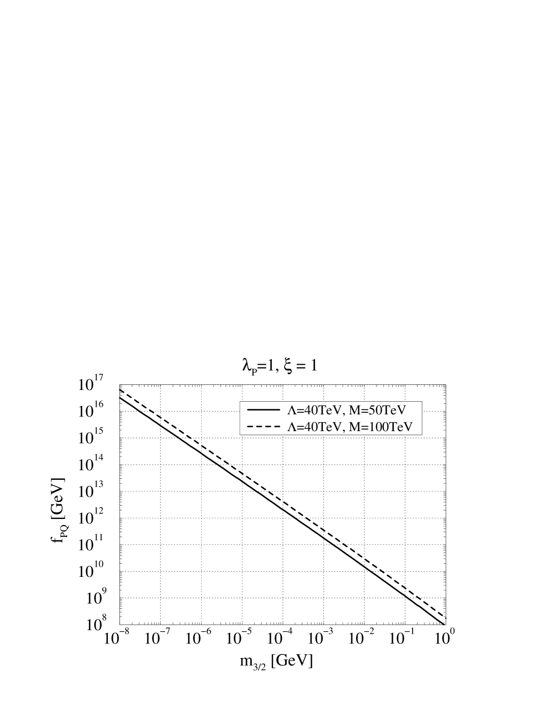
FIG. 1.: Values of the PQ breaking scale $f_{PQ}$. Parameters for the messenger sector are listed in the figure.

FIG. 2.: The vacuum diagram induced by the D-term scalar potential. $\widetilde{q}_{\pm}$ are the messenger squarks and $\widetilde{Q}_{1,2}$ are the PQ squarks.

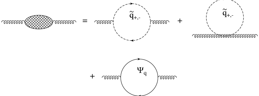
FIG. 3.: The one-loop diagrams of the vacuum polarization induced by the messenger multiplets. $\widetilde{q}_{\pm}$ are the messenger squarks and $\Psi_{q}$ denotes the messenger quark.

(a)          (b)          (c)

FIG. 4.: The vacuum diagrams with gluon. $\widetilde{Q}_{1,2}$ are the PQ squarks and $\Psi_{Q}$ denotes the PQ quark. A blob represents the one-loop vacuum polarization shown in Fig.3.

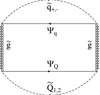
FIG. 5.: The vacuum diagram with gluino $\tilde{g}$.

REFERENCES

• [1] R.D. Peccei and H.R. Quinn, Phys. Rev. Lett. 38 (1977) 1440; Phys. Rev. D16 (1977) 1791.
• [2] J.E. Kim, Phys. Rev. Lett. 43 (1979) 103; M.A. Shifman, A.I. Vainshtein and V.I. Zakharov, Nucl. Phys. B166 (1980) 493.
• [3] T. Kugo, I. Ojima and T. Yanagida, Phys. Lett. B135 (1984) 402.
• [4] G.F. Giudice and R. Rattazzi, hep-ph/9801271.
• [5] M. Dine and A.E. Nelson, Phys. Rev. D48 (1993) 1277;
M. Dine, A.E. Nelson and Y. Shirman, Phys. Rev. D51 1362 (1995);
M. Dine, A.E. Nelson, Y. Nir and Y. Shirman, Phys. Rev. 53 2658 (1996).
• [6] K.-I. Izawa and T. Yanagida, Prog. Theor. Phys. 95 (1996) 829;
K. Intriligator and S. Thomas, Nucl. Phys. B473 (1996) 121.
• [7] N. Arkani-Hamed, G.F. Giudice, M.A. Luty and R. Rattazzi, hep-ph/9803290.
• [8] M.S. Turner, Phys. Rev. D33 (1986) 889.
• [9] E.W. Kolb and M.S. Turner, The Early Universe, Addison-Wesley (1990).
• [10] H.T. Janka, W. Keil, G. Raffelt and D. Seckel, Phys. Rev. Lett. 76 (1996) 2621.
• [11] K. Rajagopal, M.S. Turner and F. Wilczek, Nucl. Phys. B358 (1991) 447.
• [12] T. Moroi, H. Murayama and M. Yamaguchi, Phys. Lett. B303 (1993) 289.
• [13] A. de Gauvea, T. Moroi, and H. Murayama, Phys. Rev. D56 (1997) 1281.
• [14] H.B. Kim and J.E. Kim, Nucl. Phys. B433 (1995) 421.
• [15] S. Chang and H.B. Kim, Phys. Rev. Lett. 77 (1996) 591.
• [16] E. Holtmann, M. Kawasaki, K. Kohri and T. Moroi, hep-ph/9805405.
• [17] D.J. Fixsen et al, Astrophys. J. 473 (1996) 473.
• [18] M. Kawasaki and T. Yanagida, Phys. Lett. B399 (1997) 45.
• [19] E.J. Chun, H.B. Kim and J.E. Kim, Phys. Rev. Lett. 72 (1994) 1956.
• [20] T. Goto and M. Yamaguchi, Phys. Lett. B276 (1992) 103.
• [21] E.J. Chun, J.E. Kim and H.P. Nilles, Phys. Lett. B287 (1992) 123.
• [22] E.J. Chun and A. Lukas, Phys. Lett. B357 (1995) 43.
• [23] T. Asaka and M. Yamaguchi, in preparation.
Refer to caption