Meson Screening Masses in the Interacting QCD Plasma

Abstract

The meson screening mass in the pseudoscalar channel is calculated from the momentum dependent meson spectral function, using HTL fermionic propagators. A careful subtraction procedure is required to get an UV finite result. It is shown that in the whole range of temperatures explored here the HTL screening mass stays above the non-interacting result, slowly approaching the value $m_{\textrm{scr}}=2\sqrt{\pi^{2}T^{2}+m_{\infty}^{2}}$, where $m_{\infty}^{2}$ is the HTL asymptotic thermal quark mass. Our analysis leads to a better understanding of the excitations of QGP at sufficiently large temperatures and may be of relevance for interpreting lattice results.

and

1 Introduction

This work is devoted to the study of mesonic screening masses, which can be defined as the inverse screening length characterizing the exponential falloff of the mesonic spatial correlator. The importance of their evaluation in order to identify the relevant degrees of freedom in hot and dense QCD was first pointed out in [1, 2, 3], where the screening masses of mesons and nucleons were calculated on the lattice. More recent results can be found in [4, 5, 6, 7, 8, 9].

Though obtained in different discretization schemes, some common features characterize the results of all the above studies. At high temperature chiral simmetry appears to be restored: $\pi$ and $\sigma$, $\rho$ and $a_{1}$, $N_{+}$ (even-parity nucleon) and $N_{-}$ (odd-parity nucleon) turn out to be degenerate. As the temperature increases meson and baryon screening masses approach their ideal gas value of $2\pi T$ and $3\pi T$, respectively. Finally, while the screening mass of the vector mesons approaches the non-interacting result immediately above the phase transition (hence, the presence of resonant states in this channel seems to be ruled out), the result for the $\pi$ and $\sigma$ mesons stays below the ideal gas value up to higher temperatures.
Thus, $\pi$ and $\sigma$ states could possibly survive in the deconfined phase as collective excitations and be identified with the soft modes of the chiral phase transition, as first proposed in [10]. In this connection, the presence of meson-like excitations above $T_{c}$ has been also investigated within an effective PNJL model [11].

Which are then the active degrees of freedom in the QGP phase, leading to the correct interpretation of the data obtained both in the heavy-ion experiments and in lattice simulations?
For what concerns energy densities not too far from the deconfinement transition, the ones presently achievable in the heavy-ion collision experiments, the possible presence of a huge set of neutral and colored bound states surviving up to temperatures of order $\sim 2T_{c}$, has been proposed  [12, 13, 14, 15] as being able to give a unified interpretation of different experimental evidences: large cross sections, small mean free paths, perfect fluid behavior, fast thermalization, elliptic flow, etc. Actually neither the theoretical description of the QGP thermodynamics in terms of bound states [16, 17], nor the interpretation of the experimental data in terms of fast thermalization and perfect fluid behavior [18] is universally accepted.

While the features of the system just above $T_{c}$ are still under debate, at higher temperatures, starting from $T\sim 3T_{c}$, the relevant degrees of freedom should be weakly interacting quarks and gluons. In this regime, resummation schemes based on the Hard Thermal Loop (HTL) approximation were developed. Different thermodynamical observables turned out to be well described [19, 20, 21] (in particular the slow approach of the entropy, pressure and energy density to their ideal gas value is well reproduced) in terms of resummed quark and gluon propagators. The latter imply a rich structure of many-body phenomena: thermal masses, collective excitations (plasminos and longitudinal gluons) and Landau damping.
It is then of interest to investigate what these dressed degrees of freedom, which, for large enough temperatures, nicely reproduce the QGP thermodynamics, imply for the correlation of hadronic excitations.

In this paper, extending the work done in [24, 25] where the HTL meson spectral functions (MSFs) at zero and finite momentum were evaluated, we address the calculation of the $z-$axis correlator of mesonic currents. As we will show, from the large distance behavior of the correlator one can extract the screening mass of the meson. We limit ourselves to the pseudoscalar channel where, as in [24, 25], the computation “simply” requires the convolution of two HTL resummed quark propagators.
Though the evaluation of hadronic screening masses is a major achievement of lattice studies of the degrees of freedom characterizing the hot QCD (the large number of lattice sites available along the spatial directions allows one to study the large distance behavior of the correlators), analytical approaches are not so common in the literature.

The large distance behavior of hadronic correlators in the high temperature limit was first discussed in [26, 27]. The full analytical study of the spatial mesonic correlations was first addressed (to our knowledge) in the non interacting case in Ref. [28]. Effects of the interaction on the meson screening masses were analyzed, for example, in Refs. [29, 30, 31, 32, 33] within a dimensional reduction framework. A positive correction of order $g^{2}T$ to the non-interacting result $m^{0}_{\textrm{scr}}=2\pi T$ was found within this kind of approach. We will compare our numerical results to the above mentioned ones.
A study of the screening masses in the NJL model was presented in [34], whose main result (beyond stressing the huge numerical difficulty of the calculation) is to show how in the scalar and pseudoscalar channels the value of the screening mass in the deconfined phase stays below the non-interacting result, thus reflecting the presence of non-trivial correlations. This seems to agree with the lattice results and to support the presence of pion and sigma excitations for temperatures slightly larger than $T_{c}$, representing the soft modes of the chiral phase transition.

Our paper is organized as follows. We shortly review in Sec. 2 the basic definitions of the mesonic operators, correlators and spectral functions addressed in this work. In Sec. 3 we discuss how to get an UV finite result for the $z$-axis correlator in the non-interacting case and then we present the results obtained from the finite momentum HTL meson spectral function. Finally, in Sec. 4, we summarize our results and discuss how they compare to the ones obtained in independent approaches, both in the continuum and on the lattice.

2 Mesonic spatial correlation function

An interesting quantity to extract informations on the properties of hot QCD is the correlator of currents carrying the proper quantum numbers to create/destroy mesons. In practice, in the imaginary time formalism (which allows to study equilibrium properties in thermal field theory), one has to compute the following thermal expectation value

$${\rm G}_{M}(-i\tau,\boldsymbol{x})\equiv\langle\widetilde{J}_{M}(-i\tau,\boldsymbol{x})\widetilde{J}_{M}^{\dagger}(0,\boldsymbol{0})\rangle\,,$$ (1)

which provides information on how fluctuations of mesonic currents are correlated. In the above $\tau\in[0,\beta=1/T]$, while

$$\widetilde{J}_{M}(-i\tau,\boldsymbol{x})\equiv J_{M}(-i\tau,\boldsymbol{x})-\langle J_{M}(-i\tau,\boldsymbol{x})\rangle\;,$$ (2)

denotes the fluctuation of the current operator

$$J_{M}(-i\tau,\boldsymbol{x})=\bar{q}(-i\tau,\boldsymbol{x})\Gamma_{M}q(-i\tau,\boldsymbol{x})\;,$$ (3)

being $\Gamma_{M}=1,\gamma^{5},\gamma^{\mu},\gamma^{\mu}\gamma^{5}$ for the scalar, pseudoscalar, vector and pseudovector channels, respectively.

The correlator in Eq. (1) is conveniently expressed through its Fourier components according to:

$${\rm G}_{M}(-i\tau,\boldsymbol{x})=\frac{1}{\beta}\sum_{n=-\infty}^{+\infty}\int\frac{d^{3}p}{(2\pi)^{3}}e^{-i\omega_{n}\tau}e^{i\boldsymbol{p}\cdot\boldsymbol{x}}G_{M}(i\omega_{n},\boldsymbol{p})\;,$$ (4)

where $\omega_{n}=2n\pi T$ ($n=0,\pm 1,\pm 2\dots$) are the bosonic Matsubara frequencies.

The correlator in Fourier space can be written in term of its spectral density through the following representation

$$G_{M}(i\omega_{n},\boldsymbol{p})=-\int\limits_{-\infty}^{+\infty}d\omega\frac{\sigma_{M}(\omega,\boldsymbol{p})}{i\omega_{n}-\omega}\quad\Rightarrow\quad\sigma_{M}(\omega,\boldsymbol{p})=\frac{1}{\pi}\textrm{Im}\,G_{M}(\omega+i\eta,\boldsymbol{p}),$$ (5)

showing the link between the Meson Spectral Function (MSF) $\sigma_{M}$ and the retarded correlator.

On general grounds one expects the large distance correlations to be exponentially suppressed, the coefficient governing this damping being identified with the mass of the (mesonic) excitation, not necessarily corresponding to a bound state. For example the asymptotic high temperature value $2\pi T$, already mentioned in the Introduction for the meson screening mass, refers to the propagation of a non-interacting $q\bar{q}$ pair, each of the two particles carrying the minimal fermionic Matsubara frequency $\pi T$.
Before proceeding in the calculations we wish to stress that the introduction of a thermal bath establishes a privileged reference frame. Lorentz invariance is then lost and the result obtained from the correlation along the $\tau$-axis (usually referred to as dynamical mass) will not necessarily be equal to the one arising from the $z$-axis correlator (screening mass). The latter is a quantity which is most easily extracted from lattice calculations, through the analysis of the exponential damping of the following correlator:

$$\mathcal{G}_{M}(z)\equiv\int\limits_{0}^{\beta}d\tau\int d\boldsymbol{x_{\perp}}{\rm G}_{M}(-i\tau,\boldsymbol{x_{\perp}},z)\;,$$ (6)

which for large distances is expected to display a behavior like:

$$\mathcal{G}_{M}(z)\underset{z\to+\infty}{\sim}e^{\displaystyle{-m_{\textrm{scr}}z}}\;.$$ (7)

We notice that the integrations in Eq. (6) select the components in Fourier space corresponding to vanishing Matsubara frequency and transverse momentum. Hence one can write:

$$\mathcal{G}_{M}(z) = \int\limits_{-\infty}^{+\infty}\frac{dp_{z}}{2\pi}e^{\displaystyle{ip_{z}z}}G_{M}(p_{0}\!=\!0,\boldsymbol{p_{\perp}}\!\!=\!0,p_{z})$$ (8)

$$= \int\limits_{-\infty}^{+\infty}\frac{dp_{z}}{2\pi}e^{\displaystyle{ip_{z}z}}\int_{-\infty}^{+\infty}d\omega\frac{\sigma_{M}(\omega,\boldsymbol{p_{\perp}}\!\!=\!0,p_{z})}{\omega}\;,$$

where in the second line use has been made of the spectral representation given in Eq. (5). This will be the starting point for the present investigation of $z$-axis correlations.

The high-energy behavior of the spectral function, $\sigma_{M}(\omega)\sim\omega^{2}$, for $\omega\to\infty$ makes the integration over $\omega$ in Eq. (8) UV divergent. This problem is already present at the level of the non-interacting theory and has to be cured through a proper subtraction procedure. In the next section we show how we have solved this problem when quark and antiquarks propagating in the QGP are described by HTL propagators. .

3 Mesonic screening masses: HTL results

Before addressing the HTL calculation of the $z$-axis meson correlator, we briefly recall the essential aspects of the non-interacting result presented in [28]. The free correlator is written as the sum of two terms:

$$\mathcal{G}^{(0)}(z)=\mathcal{G}_{{\rm vac}}^{(0)}(z)+\mathcal{G}_{{\rm matt}}^{(0)}(z)\;.$$ (9)

The first one, temperature independent, describes the process in which the external probe with the quantum numbers of a meson excites a $q\bar{q}$ pair from the vacuum. The second one accounts for the presence of a medium (the thermal bath) which, on the one side, introduces a Pauli-blocking factor for the $q\bar{q}$ excitation; on the other side, it allows a second process (not possible in the vacuum), namely the absorption of the external probe by a (anti-)quark from the thermal bath, which is then promoted to an unoccupied single-particle state.
The expression for the vacuum piece (employing Pauli-Villars regularization in the intermediate steps) is found to be (in the case $N_{f}=2$):

$$\mathcal{G}_{{\rm vac}}^{(0)}(z)=\frac{N_{c}}{\pi^{2}z}m_{0}^{2}\,K_{2}(2m_{0}z)\;,$$ (10)

where $m_{0}$ is the current mass of the quark and $K_{2}$ is the modified Bessel function of order 2. The matter part, in turn, reads:

$$\mathcal{G}_{{\rm matt}}^{(0)}(z)=\frac{N_{c}}{2\pi^{2}}\left(\frac{1}{z^{2}}-\frac{1}{z}\frac{\partial}{\partial z}\right)\\ \left[-m_{0}\,K_{1}(2m_{0}z)+\pi T\sum_{l=-\infty}^{+\infty}\exp\left(-2z\sqrt{(2l+1)^{2}\pi^{2}T^{2}+m_{0}^{2}}\right)\right]\;,$$ (11)

where $K_{1}$ is the modified Bessel function of order 1.
By summing the two contributions an exact cancellation of the vacuum part with the first term of the matter one occurs: notably, being $m_{0}\ll T$, this term represents the major contribution to $\mathcal{G}_{\rm matt}$ at large distances. One then finds:

$$\mathcal{G}^{(0)}(z)=\frac{N_{c}T}{2\pi}\left(\frac{1}{z^{2}}-\frac{1}{z}\frac{\partial}{\partial z}\right)\sum_{l=-\infty}^{+\infty}\exp\left(-2z\sqrt{(2l+1)^{2}\pi^{2}T^{2}+m_{0}^{2}}\right)\,,$$ (12)

which for large distances displays the following asymptotic behavior:

$$\mathcal{G}^{(0)}(z)\underset{z\to\infty}{\sim}\frac{2N_{c}T}{\pi z}\sqrt{\pi^{2}T^{2}+m_{0}^{2}}\,e^{\displaystyle{-2z}\sqrt{\pi^{2}T^{2}+m_{0}^{2}}}.$$ (13)

This leads to the non-interacting result for the meson screening mass, which reads:

$$m_{\rm scr}^{(0)}=2\sqrt{\pi^{2}T^{2}+m_{0}^{2}}$$ (14)

and coincides with $2\pi T$ for vanishing current quark masses. This result arises from a dramatic cancellation of two terms, which otherwise would completely dominate the correlator at large distances. The possibility of analytically performing all the calculations in the free case allows to extract in a clean way the exact large distance behavior of the correlator.

In the interacting case the problem is much more involved, since the meson spectral function is obtained only numerically. ¿From Eq. (8) it appears that the $z$-axis correlator can be expressed in terms of the finite momentum MSF. In [25] we evaluated the latter in the HTL approximation in the pseudoscalar channel, which amounts to a convolution of two HTL resummed quark propagators. In the following we will limit ourselves to this case. Several non-trivial many-body processes turn out to contribute to the MSF and we refer the reader to ref. [25] for a detailed discussion of the various terms.
We then write the interacting spectral function as follows:

$$\sigma_{M}^{\rm HTL}(\omega,p_{z}) = \sigma_{M}^{\rm aux}(\omega,p_{z})-\left(\sigma_{M}^{\rm aux}(\omega,p_{z})-\sigma_{M}^{\rm HTL}(\omega,p_{z})\right)$$ (15)

$$\equiv \sigma_{M}^{\rm aux}(\omega,p_{z})-\sigma_{M}^{\rm diff}(\omega,p_{z})\,,$$

where we introduced the auxiliary MSF $\sigma_{M}^{\rm aux}$. For the latter we made the following choice. We employ the expression one gets in the free case from the convolution of two massive quark propagators, leading for the $z$-axis correlator to the result given in Eq. (12). For the mass of the quarks we replace the free value $m_{0}$ by the HTL asymptotic thermal quark mass $m_{\infty}=\sqrt{2}m_{q}=g(T)T/\sqrt{3}$, $m_{q}$ being the thermal gap mass appearing in the fermionic spectrum. Indeed, in the HTL approximation, the asymptotic thermal mass governs the large-momentum regime of the quark dispersion relation. Our choice guarantees a convergent high-energy behavior for the difference $\sigma_{M}^{\rm diff}(\omega,p_{z})$, which makes the integration of the latter in Eq. (8) well defined.

In Figs. 1-3, we show the $\omega$ dependence of all the contributions to Eq. 15 for a few momenta $p_{z}$, for the case $T=2T_{c}$. The numerical calculations were performed up to $\omega=2500\,{\rm fm}^{-1}$ in order to check the correct high-energy limit of the difference between the HTL and the auxiliary spectral functions. Such a difference is well behaved and, as $\omega$ grows, goes smoothly to zero, as we can see in Figs. 4-6.

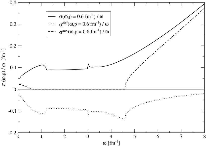
Figure 1: The finite momentum pseudoscalar MSF divided by $\omega$ together with the auxiliary one and their difference, for $p_{z}=0.6\;{\rm fm}^{-1}$ and $T=2T_{c}$.

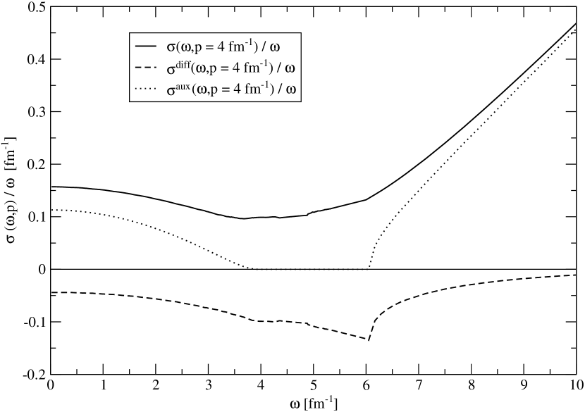
Figure 2: The finite momentum pseudoscalar MSF divided by $\omega$ together with the auxiliary one and their difference, for $p_{z}=4.0\;{\rm fm}^{-1}$ and $T=2T_{c}$.

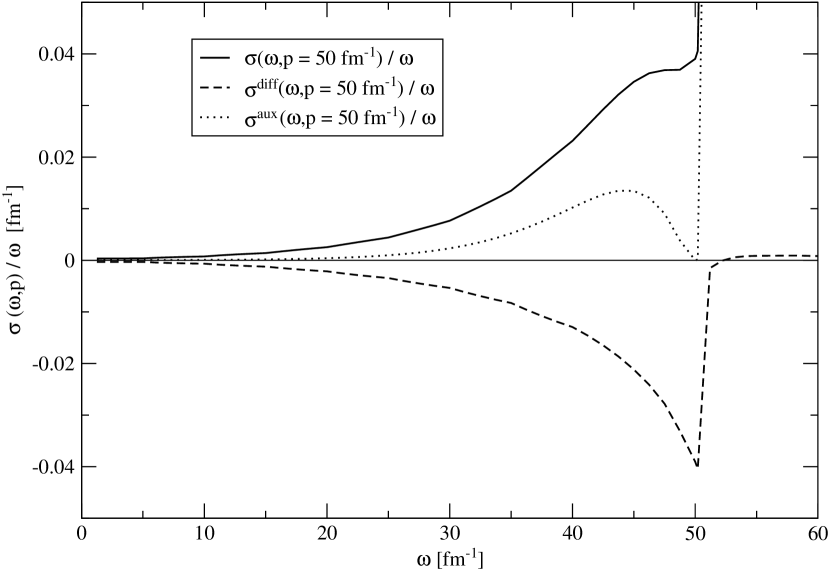
Figure 3: The finite momentum pseudoscalar MSF divided by $\omega$ together with the auxiliary one and their difference, for $p_{z}=50.0\;{\rm fm}^{-1}$ and $T=2T_{c}$.

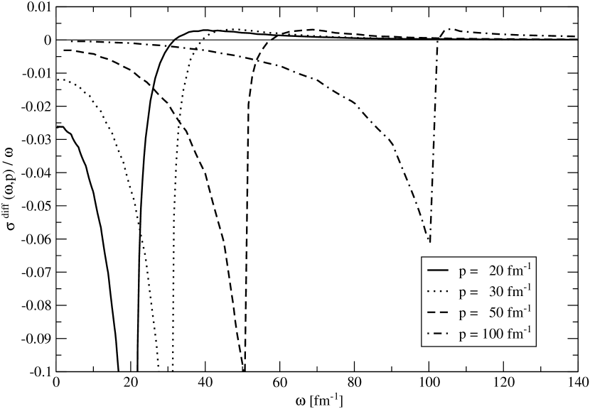
Figure 4: The difference between the auxiliary and the HTL pseudoscalar MSF divided by $\omega$ for momenta $p_{z}=20-100\;{\rm fm}^{-1}$ and $T=4T_{c}$.

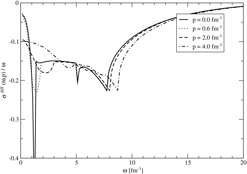
Figure 5: The same as in Fig. 4 but for momenta $p_{z}=0-4\;{\rm fm}^{-1}$ and for small $\omega$.

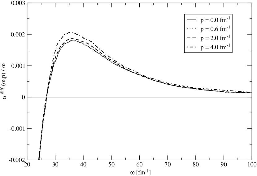
Figure 6: The same as in Fig 5 but for large $\omega$.

The $z$-axis correlator accordingly reads:

$$\mathcal{G}^{\rm HTL}(z)=\mathcal{G}^{\rm aux}(z)-\mathcal{G}^{\rm diff}(z)\,,$$ (16)

where $\mathcal{G}^{\rm aux}(z)$ is given by Eq. (12) after making the replacement $m_{0}\to m_{\infty}$, while $\mathcal{G}^{\rm diff}(z)$ is obtained by numerically evaluating

$$\mathcal{G}^{\rm diff}(z)=\int\limits_{-\infty}^{+\infty}\frac{dp_{z}}{2\pi}\;e^{\displaystyle{ip_{z}z}}\;G^{\rm diff}(p_{z})=\int\limits_{-\infty}^{+\infty}\frac{dp_{z}}{2\pi}\;e^{\displaystyle{ip_{z}z}}\int_{-\infty}^{+\infty}\frac{d\omega}{\omega}\;\sigma^{\rm diff}_{PS}(\omega,p_{z})\;,$$ (17)

the integration over $\omega$ being now well defined.
¿From Eq. (17) it clearly appears that the full determination of $\mathcal{G}^{\rm diff}(z)$ would in principle require performing the Fourier Transform (FT) of a function that we know only numerically, after summing a huge set of different contribution which are listed in Ref. [25]. In the present work, however, we are only interested in the determination of the coefficient which governs the exponential damping of $\mathcal{G}^{\rm diff}(z)$. Hence we will limit ourselves to evaluate with high precision the large $z$ behaviour of the latter.
For this purpose it appears then more convenient to employ the following procedure: we perform a fit of $G^{\rm diff}(p_{z})$ with a function whose FT in coordinate space is known and displays an exponential decay at large distances. For the sake of simplicity, for the fitting function we choose

$$G^{\rm diff}(p_{z})=-\sum_{i=1}^{2}\frac{2m_{i}c_{i}}{m^{2}+p_{z}^{2}}\;,$$ (18)

which leads to a $z$-axis correlator with the following functional form:

$$\mathcal{G}^{\rm diff}(z)=-\sum_{i=1}^{2}c_{i}e^{-m_{i}z}\;.$$ (19)

The above, indeed, is a simple multi-exponential fit, which is generally used to extract the masses of physical states with given quantum numbers from the study of lattice correlators.
We are aware that there is a priori no reason, for the above expression, to be the correct functional form of $\mathcal{G}^{\rm diff}(z)$, as it can be guessed, for example, by looking at the free result in Eq. (12). This assumption could obviously introduce some bias in our results. Hence, while we are confident that at large distances the correlator is dominated by a single decreasing exponential, controlled by the smallest between the two parameters $m_{i}$, we do not attach a real physical meaning to the other coefficients of the fitting function.

In order to clarify our fitting procedure let us start by considering the large distance behavior of the non-interacting $z$-axis correlator. ¿From Eq. (12), for the case $m_{0}=0$, it follows that the latter can be conveniently expressed in the following form:

$$\mathcal{G}^{(0)}(z) = c_{1}(z)e^{-(2\pi T)z}+c_{2}(z)e^{-(6\pi T)z}+\dots$$ (20)

$$= c_{1}(z)e^{-(2\pi T)z}\left(1+\frac{c_{2}(z)}{c_{1}(z)}e^{-(4\pi T)z}+\dots\right)\,,$$

where the $c_{i}(z)$ are functions displaying only a mild dependence on $z$ (compared to an exponential), which in principle can be obtained by matching the above expression with Eq. (12). Then one expects the $z$-dependence being dominated by the first exponential for distances such that

$$(4\pi T)\,z\gg 1\quad\Longleftrightarrow\quad z\gg\frac{1}{4\pi T}\,.$$ (21)

We believe it to be a reasonable assumption that these considerations remain essentially true also in the interacting case. Then, from

$$\mathcal{G}^{\rm diff}(z)=\int\limits_{-\infty}^{+\infty}\frac{dp_{z}}{2\pi}\;e^{\displaystyle{ip_{z}z}}\;G^{\rm diff}(p_{z})$$ (22)

it follows that in order to correctly reproduce the large $z$ behavior of $\mathcal{G}(z)$ one needs a careful determination of $G(p_{z})$ up to $p_{z}\sim 1/z$. Contributions from $p_{z}\gg 1/z$ are in fact suppressed by the oscillations of the integrand. Hence, from Eq. (21), one can assume that the numerical evaluation of the screening mass from a fit reconstruction of $G(p_{z})$ requires a sufficiently large number of data points for $p_{z}\mathrel{\mathop{\kern 0.0pt\hbox to0.0pt{\raise 0.86108pt\hbox{$<$}\hss}}\lower 3.87495pt\hbox{\kern-1.90002pt$\sim$}}4\pi T$. On the other hand one should not extend the fit to too large values of $p_{z}$, otherwise the lighest mass would no longer control the $z$-behavior.
Of course a more precise determination of the range over which the fit has to be performed cannot be obtained through these semi-quantitative considerations. In practice, in fitting $G^{\rm diff}(p_{z})$ we adopted the following procedure. For each temperature we varied the maximum value of $p_{z}$ in a “reasonable range”. After checking that the value of the lightest mass ($m_{1}$) was sufficiently robust with respect to the arbitrary choice of $p_{z}^{\rm max}$ (i.e. displaying very modest variations), for each temperature we took a weighted average of the different values.

The results for $m_{1}$ are reported in Table 1, together with the estimate of the error resulting from the fitting procedure and the range over which we varied $p_{z}^{\rm max}$. As a further check of the robustness of the values of $m_{1}$ thus obtained, for each temperature, we extended our fit to larger values of $p_{z}$, introducing a third decreasing exponential. In all the cases we found that the values of $m_{1}$ obtained with this three-mass fit are indeed consistent with the ones given in Table 1.

$T/T_{c}$	$m_{1}\,({\rm fm}^{-1})$	$\delta m_{1}\,({\rm fm}^{-1})$	$p_{max}\,({\rm fm}^{-1})$
1	6.754	0.016	15$\div$50
2	13.415	0.015	30$\div$100
4	26.213	0.043	40$\div$200
10	65.84	0.41	200$\div$300

Table 1: The coefficient $m_{1}$ extracted from the fit of $G^{\rm diff}(p_{z})$ for the different temperatures explored, together with the range of momenta over which the fit has been performed.

The accuracy of the fit is shown in Figs. 7-10 for different temperatures. In all figures the numerical calculation of $G^{\rm diff}(p_{z})$ (open circles) is compared with the smooth fitting function.

Figure 7: $G^{\rm diff}(p_{z})$ [in fm^-2] for the temperature $T/T_{c}=1$.

Figure 8: $G^{\rm diff}(p_{z})$ [in fm^-2] for the temperature $T/T_{c}=2$.

Figure 9: $G^{\rm diff}(p_{z})$ [in fm^-2] for the temperature $T/T_{c}=4$.

Figure 10: $G^{\rm diff}(p_{z})$ [in fm^-2] for the temperature $T/T_{c}=10$.

In Table 2 we collect our results, at different temperatures, for the screening mass: together with the non-interacting result ($m_{\rm free}=2\pi T$) we report the auxiliary HTL mass $m_{\rm{scr}}^{\rm aux}=2\sqrt{\pi^{2}T^{2}+m_{\infty}^{2}}$ and the lightest mass arising from our fit of ${\mathcal{G}}^{\rm diff}(z)$. Clearly the screening mass ($m_{\rm scr}^{\rm HTL}$), governing the exponential decay of the HTL $z$-axis correlator ${\mathcal{G}}^{\rm HTL}(z)$, is given by:

$$m_{\rm scr}^{\rm HTL}={\rm min}(m_{\rm scr}^{\rm aux},m_{1})\;.$$ (23)

The Table shows that at all temperatures $m_{1}$ turns out to be smaller than $m_{\rm scr}^{\rm aux}$ but larger than $m_{\rm free}$; hence it has to be assumed as the ”true” HTL screening mass. Notice that, independently on the result of the fit, $m_{\rm scr}^{\rm aux}$ sets an upper cutoff to the HTL screening mass.

$T/T_{c}$	$2\pi T\,({\rm fm}^{-1})$	$m_{\rm scr}^{\rm aux}\,({\rm fm}^{-1})$	$m_{1}\,({\rm fm}^{-1})$	$m_{\rm scr}^{\rm HTL}\,({\rm fm}^{-1})$
1	6.432	7.08	6.754	6.754
2	12.864	13.64	13.415	13.415
4	25.728	26.86	26.213	26.213
10	64.32	66.45	65.84	65.84

Table 2: The screening masses governing the exponential decay of the non-interacting correlator, of the auxiliary one, of the difference between the HTL and the auxiliary correlators, respectively. In the last column we show the HTL screening mass.

For the sake of completeness, we report in Table 3 the average values found for the other fit parameters, though we do not attach any physical meaning to them, in particular to the heavier mass $m_{2}$. Notice that, since the parameter $m_{2}$ is always very large, by limiting the range of the fit to not too large values of $p_{z}$ one can indeed fit equally well the data by a constant (which would correspond to a contact term in coordinate space) plus a single decreasing exponential. We checked that in this case the value of $m_{1}$ results slightly larger than the one we quote in Tables 1 and 2 arising from the two-mass fit, and approach $m_{\rm scr}^{\rm aux}$ even faster.

$T/T_{c}$	$c_{1}\pm\delta c_{1}\,({\rm fm}^{-3})$	$m_{2}\pm\delta m_{2}\,({\rm fm}^{-1})$	$c_{2}\pm\delta c_{2}\,({\rm fm}^{-3})$
1	0.364$\pm$0.001	195.5$\pm$4.0	15.3$\pm$0.3
2	1.754$\pm$0.003	291.3$\pm$1.7	54.4$\pm$0.3
4	10.13$\pm$0.03	377.6$\pm$1.7	208.3$\pm$0.8
10	126.1$\pm$1.5	527.4$\pm$6.6	1301.0$\pm$10.3

Table 3: The weighted average of the other fit coefficients extracted from $G^{\rm diff}(p_{z})$ for the different temperatures explored.

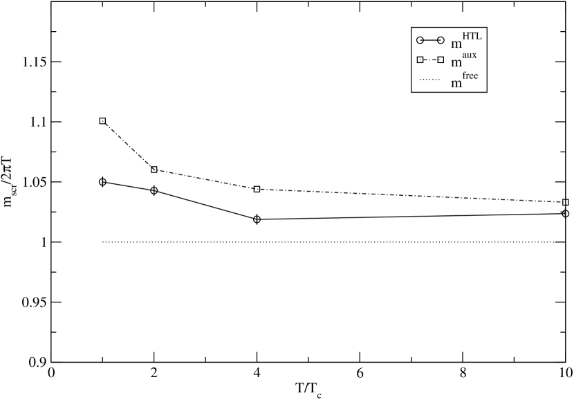
Figure 11: The temperature dependence of the HTL result for the meson screening mass, together with the auxiliary one, in units of the non-interacting value $2\pi T$.

In Fig. 11 we plot the HTL and auxiliary screening masses in units of the non-interacting value $2\pi T$ as a function of the temperature. One can see that for large temperatures, the HTL screening mass approaches the auxiliary result

$$m_{\rm scr}^{\rm HTL}{\simeq}m_{\rm scr}^{\rm aux}=2\sqrt{\pi^{2}T^{2}+m_{\infty}^{2}}\;,$$ (24)

where $m_{\infty}$ is the asymptotic thermal mass of the quark. The high temperature behavior we have found deserves a discussion on its physical origin. The main effect of the interaction is to dress the quarks with a thermal mass. Yet we remind that the HTL propagator respects chiral invariance, though being dominated for large momenta by a quasiparticle pole with the dispersion relation of a massive particle.

It is indeed interesting to evaluate the lowest order correction to the non-interacting result for the screening mass, which can be obtained by expanding Eq. (24) for $m_{\infty}\ll\pi T$ (as it is indeed the case, since $m_{\infty}=gT/\sqrt{3}$). One gets, for large temperatures:

$$m_{\rm scr}^{\rm HTL}\simeq 2\pi T+\frac{1}{3\pi}g^{2}T\;.$$ (25)

One can compare this result with the one obtained in [32, 33] which can be cast in the form:

$$m_{\rm scr}\simeq 2\pi T+\left(\frac{1}{3\pi}+\Delta\right)g^{2}T\;,$$ (26)

$\Delta$ being an additional correction term, to the same order.

Our result has been obtained through the convolution of two HTL quark propagators, somehow assuming that the relevant degrees of freedom in the high-temperature phase of QCD are dressed quasiparticles. This leads (assuming the asymptotic high-temperature behavior numerically found to be correct) to a non-perturbative result for the meson screening mass, which implicitly contains infinite powers of $g^{2}$.

In [32, 33] the approach is completely different. These authors do not use resummed propagators. An effective $(2+1)$ dimensional Lagrangian is built, in which the relevant degrees of freedom are the lowest fermionic Matsubara modes and soft gluons. Within this approach the result given in Eq. (26) is found for the screening mass, where the coefficient of the $g^{2}T$ term results from the sum of two pieces. The first one arises from a correction to the mass of the fermionic modes and coincides with our result, to the extent that the HTL result is expanded perturbatively; the second term instead ($\Delta$) is related to vertex and quark self-energy corrections, arising from soft gluons, which are ignored in our approach. Indeed we remind the reader that the pseudoscalar vertex receives no HTL correction and, in the evaluation of HTL self-energy diagrams, one considers the loop integrals being dominated by hard internal momenta.

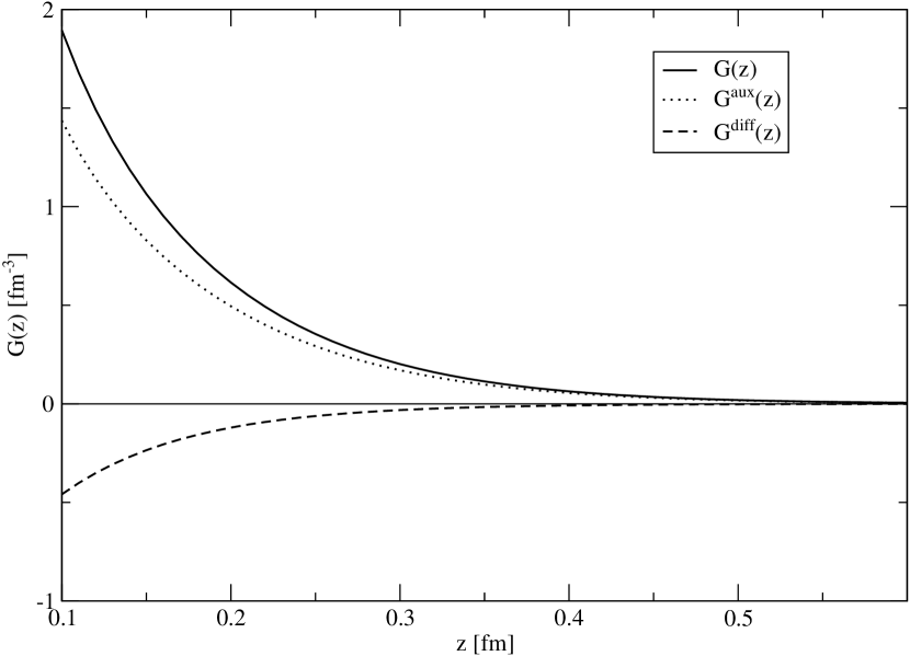
Figure 12: The final result for the HTL $z$-axis correlator $\mathcal{G}^{\rm HTL}(z)$ (continuous line) obtained, according to Eq. (16), through the difference between the auxiliary correlator $\mathcal{G}^{\rm aux}(z)$ and $\mathcal{G}^{\rm diff}(z)$, which arises from our simple exponential fit. Only the large distance behavior should be trusted. The figure refers to the case $T=2T_{c}$

Both our approach and the one employed in [32, 33] agree in predicting a small positive correction of order $g^{2}T$ to the non-interacting result for the meson screening mass, in contrast with the lattice results available so far. The above discussed origin of the small discrepancy, between the two approximation schemes, which affects the exact numerical coefficient of $g^{2}T$, makes, in our opinion, this qualitative trend of the results rather robust and represents a challenge for lattice studies.

Finally, in Fig. 12 we display the behavior of the spatial correlator $\mathcal{G}(z)$ for the case $T=2T_{c}$ obtained by combining togheter the auxiliary correlator $\mathcal{G}^{\rm aux}(z)$ (evaluated from Eqs. (16) and (12) ) and the result for $\mathcal{G}^{\rm diff}(z)$ arising from our two-mass fit.

4 Conclusions

In this paper we have addressed the numerical evaluation of the screening mass of a (pseudoscalar) meson in the QGP phase of QCD, i.e. the quantity which governs the large-distance exponential decay of the correlations of mesonic current operators.

We have presented results obtained in the Hard Thermal Loop approximation. While the pseudoscalar vertex does not receive HTL corrections, for the fermionic lines the HTL resummed propagators have been employed. In this scheme the spectral density of the quark correlator is characterized by two stable quasi-particle poles (normal quark and plasmino mode) for time-like momenta, and by a continuum contribution in the space-like domain related to the damping of the quark due to its interaction with the other particles of the thermal bath (Landau damping). In a previous publication [25] we have shown in detail that this structure of the fermionic propagator gives rise to an extremely rich and complex set of many-body processes contributing to the finite-momentum spectral function of a meson in the QCD deconfined phase.

Here we employed the previous results to derive the spatial meson correlator, limiting the discussion to the asymptotic propagation along the $z$-axis and presenting numerical results for the screening mass of a pseudoscalar meson.
We discussed in the text how we managed to deal with the problem of the UV divergences (arising from the $\omega^{2}$ growth of the MSF at high energy) which one encounters in the calculation: the latter are overcome through a careful subtraction procedure which takes advantage of how this problem has been solved in the non-interacting case.
Our numerical results shows that the HTL screening mass, in the explored temperature range, turns out to be a few percent higher than the non-interacting value $2\pi T$, (very) slowly approaching it from above as the temperature increases.
We have also compared our results with the ones obtained in another analytical approach based on a dimensional-reduced lagrangian [32, 33], which also finds a positive correction of order $g^{2}T$ to the non-interacting result. Quite interestingly, once we expand perturbatively what comes out from our numerical findings for the asymptotic high-temperature behavior of the screening mass, we also get a correction to the free result of order $g^{2}T$. The coefficient of this correction differs from the one found in [32, 33] since, in the HTL approximation, soft gluons corrections are neglected.

Concerning the lattice data available so far, to our knowledge, all the screening masses extracted from them approach the non-interacting value $2\pi T$ from below. This indeed appears in conflict with the studies performed in the continuum by us and, within a different framework, by the authors of Ref. [32, 33]. Whether this is related to limitations of the present lattice results or by a breakdown of the approximations assumed in both the continuum studies (based on a separation of the scales $T$, $gT$ and $g^{2}T$, which is rigorously defined only in the regime $g\ll 1$) is an open question.
Indeed the positive correction found in the analytical approaches mainly arises from the thermal mass aquired by the quark modes at finite temperature, a fact which appears sound. On the other hand, the lattice results available so far do not extend up to very high temperatures. Hence it is possible that the apparent mismatch between the lattice and the continuum results is due to the fact that the weak coupling regime, which makes the approximations and the separation of momentum scales justified, is achieved only at temperatures not yet covered by the lattice studies. However a more careful investigation of the possible limitations of the lattice results available so far might be of interest.

Appendix A The running of the coupling

Our numerical results refer to the case $N_{f}=2$. The transition temperature, following [35], has been set to the value $T_{c}=202$ MeV. The ratio $T_{c}/\Lambda_{\overline{MS}}=0.7721$ for the $N_{f}=2$ case is taken from Refs. [36, 37, 38]. The running of the gauge coupling is given by the two-loop perturbative beta-function, leading to the expression:

$$g^{-2}(T)=2b_{0}\log{\frac{\mu}{\Lambda_{\overline{MS}}}}+\frac{b_{1}}{b_{0}}\log\Big{\{}2\log{\frac{\mu}{\Lambda_{\overline{MS}}}}\Big{\}}$$ (27)

where $b_{0}=\frac{1}{16\pi^{2}}\Big{(}11-2\frac{N_{f}}{3}\Big{)}$, $b_{1}=\frac{1}{(16\pi^{2})^{2}}\Big{(}102-38\frac{N_{f}}{3}\Big{)}$ The renormalization scale $\mu$ is usually taken to be of the order of the temperature, which, apart from $\Lambda_{QCD}$, represents the only physical scale entering into the problem. For what concerns its precise numerical value one should, in principle, let it vary within a reasonable range in order to get an estimate of the theoretical uncertainty of the calculation. Here, for the sake of simplicity, due to the huge numerical work required to produce our results, we adopt the choice $\mu=1.142\pi T$ suggested in [35].

References

- [1] C. DeTar and J. Kogut, Phys. Rev. Lett. 59 (1987), 399;
- [2] C. DeTar and J. Kogut, Phys. Rev. D36 (1987), 2828;
- [3] S. Gottlieb et al., Phys. Rev. Lett. 59 (1987), 1881;
- [4] MT(c) Collaboration (K.D. Born et al.), Phys. Rev. Lett. 67 (1991), 302;
- [5] QCD-TARO Collaboration (P. de Forcrand et al.), Phys. Rev. D63 (2001), 054501;
- [6] By QCD-TARO Collaboration (Irina Pushkina et al.), Phys. Lett. B609 (2005), 265;
- [7] S. Wissel et al., PoS LAT2005 (2006), 164;
- [8] R. Gavai and S. Gupta, Phys. Rev. D67 (2003), 034501;
- [9] R. Gavai, S. Gupta and R. Lacaze; hep-lat/0609074;
- [10] T. Hatsuda and T. Kunihiro, Phys. Rev. Lett. 55 (1985), 158;
- [11] H. Hansen et al., Phys. Rev. D75 (2007), 065004;
- [12] M. Asakawa, T. Hatsuda and Y. Nakahara, Nucl. Phys. A715 (2003), 863;
- [13] M. Asakawa and T. Hatsuda, Phys. Rev. Lett. 92 (2004), 012001;
- [14] E. Shuryak, Prog. Part. Nucl. Phys. 53 (2004), :273;
- [15] E. Shuryak and I. Zahed, Phys. Rev. D70 (2004), 054507;
- [16] V. Koch, A. Majumder and J. Randrup, Phys. Rev. Lett. 95 (2005), 182301;
- [17] C.Ratti, M.A. Thaler and W. Weise, Phys. Rev. D73 (2006), 014019;
- [18] R.S. Bhalerao, J.P. Blaizot, N. Borghini and J.Y. Ollitrault, Phys. Lett. B627 (2005), 49;
- [19] J.P. Blaizot, E. Iancu and A. Rebhan, Phys. Lett. B470 (1999), 181;
- [20] J.P. Blaizot, E. Iancu and A. Rebhan, Phys. Rev. D63 (2001), 065003;
- [21] J.P. Blaizot, E. Iancu and A. Rebhan, In *Hwa, R.C. (ed.) et al.: Quark gluon plasma* 60-122. hep-ph/0303185;
- [22] J.B. Kogut, J.F. Lagaë and D.K. Sinclair, Phys. Rev. D58 (1998), 054504;
- [23] G. Aarts, C. Allton, J. Foley and S. Hands, hep-lat/0610061;
- [24] W.M. Alberico, A. Beraudo and A. Molinari, Nucl. Phys. A750 (2005), 359;
- [25] W.M. Alberico, A. Beraudo, P. Czerski and A. Molinari, Nucl. Phys. A775 (2006), 188;
- [26] V.L. Eletskii and B.L. Ioffe Sov. J. Nucl. Phys. 48 (1988), 384;
- [27] E.V. Shuryak, Rev. Mod. Phys. 65 (1993), 1;
- [28] W. Florkowski and B.L. Friman Z. Phys. A347 (1994), 271;
- [29] V. Koch, E. V. Shuryak, G.E. Brown and A.D. Jackson, Phys. Rev. D46 (1992), 3169;
- [30] V. Koch, Phys. Rev. D49 (1994), 6063;
- [31] T.H. Hansson and I. Zahed, Nucl. Phys. B374 (1992), 277;
- [32] M. Laine and M. Vepsalainen, JHEP 0402 (2004) 004.
- [33] M. Vepsalainen, hep-ph/0701250;
- [34] W. Florkowski, Acta Phys. Polon. B28 (1997), 2079;
- [35] O. Kaczmarek and F. Zantow, Phys. Rev.D71 (2005), 114510;
- [36] F. Karsch, E. Laermann, and A. Peikert, Phys. Lett. B478 (2000), 447.
- [37] M. Gockeler et al., Phys.Rev. D73 (2006) 014513,
- [38] O. Kaczmarek and F. Zantow, hep-lat/0512031.