Chiral-logarithmic Corrections to the $S$ and $T$ Parameters in Higgsless Models

Abstract

Recently, Higgsless models have proven to be viable alternatives to the Standard Model (SM) and supersymmetric models in describing the breaking of the electroweak symmetry. Whether extra-dimensional in nature or their deconstructed counterparts, the physical spectrum of these models typically consists of “towers” of massive vector gauge bosons which carry the same quantum numbers as the SM $W$ and $Z$. In this paper, we calculate the one-loop, chiral-logarithmic corrections to the $S$ and $T$ parameters from the lightest (i.e. SM) and the next-to-lightest gauge bosons using a novel application of the Pinch Technique. We perform our calculation using generic Feynman rules with generic couplings such that our results can be applied to various models. To demonstrate how to use our results, we calculate the leading chiral-logarithmic corrections to the $S$ and $T$ parameters in the deconstructed three site Higgsless model. As we point out, however, our results are not exclusive to Higgsless models and may, in fact, be used to calculate the one-loop corrections from additional gauge bosons in models with fundamental (or composite) Higgs bosons.

I Introduction

The source of electroweak symmetry breaking (EWSB), i.e. the generation of the $W^{\pm}$ and $Z^{0}$ masses, remains as one of the unanswered questions in particle physics. If the Standard Model (SM) or one of its supersymmetric (SUSY) extensions are correct, then one (or more) $SU(2)$ scalar doublets are responsible for EWSB and at least one physical Higgs boson should be discovered at the Large Hadron Collider (LHC).

Unfortunately, the Higgs mechanism as implemented in the SM has several theoretical shortcomings. The most troublesome of these is the fact that the Higgs boson mass is unstable against radiative corrections, a situation known as the large hierarchy problem. In other words, for the Higgs boson to be light (as indicated by electroweak precision measurements), its bare mass must be highly fine-tuned to cancel large loop effects from high-scale physics. In SUSY extensions, this fine-tuning is avoided due to additional particles which cancel the quadratic contributions to the Higgs boson mass from SM particles.

In the past several years, an interesting alternative to SUSY models has emerged in the form of extra-dimensional models Arkani-Hamed et al. (1998); Randall and Sundrum (1999). In most of these scenarios, the size and shape of the extra dimension(s) are responsible for solving the large hierarchy problem. In addition, variations of these models can also provide viable alternatives to the Higgs mechanism. For example, in models where the SM gauge fields propagate in a fifth dimension, masses for the $W^{\pm}$ and $Z^{0}$ bosons can be generated via non-trivial boundary conditions placed on the five-dimensional wavefunctions Csaki et al. (2004a); Cacciapaglia et al. (2005a); Nomura (2003); Csaki et al. (2004b). Since the need for scalar doublets is eliminated in such scenarios, these models have been aptly dubbed Higgsless models. The result of allowing the SM gauge fields to propagate in the bulk, however, is towers of physical, massive vector gauge bosons (VGBs), the lightest of which are identified with the SM $W^{\pm}$ and $Z^{0}$ bosons. The heavier Kaluza-Klein (KK) modes, which have the $SU(2)\times U(1)$ quantum numbers of the SM $W^{\pm}$ and $Z^{0}$, play an important role in longitudinal VGB scattering. In the SM without a Higgs boson, the scattering amplitudes for these processes typically violate unitarity around $\sim$ 1.5 TeV Lee et al. (1977). The exchange of light Higgs bosons, however, cancels the unitarity-violating terms and ensures perturbativity of the theory up to high scales. In extra-dimensional Higgsless models, the exchange of the heavier KK gauge bosons plays the role of the Higgs boson and cancels the dominant unitarity-violating terms Csaki et al. (2004a). As a result, the scale of unitarity violation can be pushed to the $\sim$ 5-10 TeV range.

The main drawback of extra-dimensional models is that they are non-renormalizable and, thus, must be viewed as effective theories up to some cutoff scale $\Lambda$ above which new physics must take over. An extremely efficient and convenient way of studying the phenomenology of five-dimensional effective theories in the context of four-dimensional gauge theories is that of deconstruction Arkani-Hamed et al. (2001); Hill et al. (2001). Deconstructed models possess extended gauge symmetries which approximate the fifth dimension, but can be studied in the simplified language of coupled non-linear sigma models (nl$\sigma$m) Appelquist and Bernard (1980); Longhitano (1980, 1981). In fact, this method allows one to effectively separate the perturbatively calculable contributions to low-energy observables from the strongly-coupled contributions due to physics above $\Lambda$. The former arise from the new weakly-coupled gauge states, while the latter can be parameterized by adding higher-dimension operators Appelquist and Bernard (1980); Longhitano (1980, 1981); Bagger et al. (1993); Perelstein (2004); Chivukula et al. (2007).

The phenomenology of deconstructed Higgsless models has been well-studied Foadi et al. (2004); Hirn and Stern (2004); Casalbuoni et al. (2004); Chivukula et al. (2004a); Perelstein (2004); Georgi (2005); Sekhar Chivukula et al. (2005a). Recently, however, the simplest version of these types of models, which involves only three “sites” Foadi et al. (2004); Perelstein (2004); Sekhar Chivukula et al. (2006), has received much attention and been shown to be capable of approximating much of the interesting phenomenology associated with extra-dimensional models and more complicated deconstructed Higgsless models Cacciapaglia et al. (2005a, b); Foadi et al. (2005); Foadi and Schmidt (2006); Chivukula et al. (2005a); Casalbuoni et al. (2005); Sekhar Chivukula et al. (2005b). The gauge structure of the three site model is identical to that of the so-called BESS (Breaking Electroweak Symmetry Strongly) which was first analyzed over twenty years ago Casalbuoni et al. (1985, 1987). Once EWSB occurs in the three site model, the gauge sector consists of a massless photon, two relatively light massive VGBs which are identified with the SM $W$ and $Z$ gauge bosons, as well as two new heavy VGBs which we denote as $W^{\prime}$ and $Z^{\prime}$. The exchange of these heavier states in longitudinal VGB scattering can delay unitarity violation up to higher scales Foadi et al. (2004).

Given the prominent role that the heavier VGBs play in the extra-dimensional and deconstructed Higgsless scenarios, it is important to assess their effects on electroweak precision observables, namely the oblique parameters ($S,T$ and $U$) Peskin and Takeuchi (1992). These parameters are defined in terms of the SM gauge boson self-energies, $\Pi^{\mu\nu}_{ij}(q^{2})$, where $(ij)$ = $(WW),(ZZ),(\gamma\gamma)$ and $(Z\gamma)$, and $q$ is the momentum carried by the external gauge bosons. Generically, the one-loop contributions to the $\Pi_{ij}$ can be split into four separate classes depending on the particles circulating in the loops: namely, those involving (i) only fermions, (ii) only scalars, (iii) a mixture of scalars and gauge bosons and (iv) only gauge bosons. Due to gauge invariance, class (i) and the sum of classes (ii) and (iii) are independent of the $R_{\xi}$ gauge used in the calculation. However, class (iv), i.e. contributions to the two-point functions from loops of gauge bosons, are $R_{\xi}$ gauge-dependent. This was shown explicitly for the case of one-loop contributions from SM gauge bosons in Ref. Degrassi and Sirlin (1992a). In that paper, the authors showed that in a general $R_{\xi}$ gauge the gauge boson self-energies depend non-trivially on the gauge parameter(s) $\xi_{i}$ ($i=W,Z,\gamma$). These dependences carry over into the calculation of the oblique parameters resulting in gauge-dependent expressions for $S,T$ and $U$ Degrassi et al. (1993). However, in a series of subsequent papers, it was shown that by isolating the gauge-dependent terms from other one-loop corrections (i.e. vertex and box corrections) and combining these with the self-energy expressions derived from the two-point functions, it is possible to define gauge-invariant forms of the self-energies and, thus, obtain gauge-invariant expressions for the oblique parameters Degrassi and Sirlin (1992b, a); Papavassiliou and Sirlin (1994); Degrassi et al. (1993). This method of extracting gauge-invariant Green’s functions from scattering amplitudes is known as the Pinch Technique (PT) Cornwall (1981, 1982); Cornwall and Papavassiliou (1989); Papavassiliou (1990).

In this paper, we generalize the results of Refs. Degrassi and Sirlin (1992b, a); Papavassiliou and Sirlin (1994); Degrassi et al. (1993) to calculate the one-loop, chiral logarithmic corrections to the oblique parameters in extra-dimensional and deconstructed Higgsless models. In our calculation of the PT self-energies, we employ the unitary gauge ($\xi\to\infty$) to define the massive VGB propagators. The attractive feature of this choice is that unphysical states (i.e. Goldstone bosons, ghosts, etc.) decouple and thus the number of diagrams is drastically reduced. Green’s functions calculated in unitary gauge are individually non-renormalizable in the sense that they contain divergences proportional to higher powers of $q^{2}$ which cannot be removed by the usual counterterms. However, when the PT is applied, these non-renormalizable terms cancel in the same manner as the gauge-dependent terms mentioned above Papavassiliou and Sirlin (1994).

The rest of this paper is organized in the following way. In Section II, we discuss the generic Feynman rules used in our calculation. We also describe in some detail the three-site Higgsless model to which we will apply our results in the following sections. Section III contains a general discussion on the Pinch Technique and its use within the unitary gauge. In Sections IV and V, we calculate the one-loop corrections needed to construct the PT self-energies in terms of generic couplings. These corrections are then assembled in Section VI where we explicitly show how to construct the PT gauge boson self-energies. Using these expressions, we calculate the leading chiral-logarithmic corrections to the $S$ and $T$ parameters in the three-site model in Section VII. The one-loop corrections to the $S$ and $T$ parameters in the three site model were first calculated in Refs. Chivukula et al. (2007); Matsuzaki et al. (2006) to which we compare our results and find excellent agreement. Finally, in Section VIII, we conclude.

II The Model(s)

Our results apply to a wide class of Higgsless models in extra-dimensional and deconstructed theories. We begin this section by outlining the types of models for which our calculation is valid. After defining the generic Feynman rules used in our calculation, we discuss the three site Higgsless model in detail and show how it fits within the framework described below.

First, assume that the model has an extended gauge symmetry of the form:

$$SU(2)\times SU(2)^{N}\times\times U(1)\,,$$ (1)

where the $U(1)$ is gauged as the $T_{3}$ component of a global $SU(2)$ and the effective four-dimensional Lagrangian for the gauge kinetic terms is:

$${\cal{L}}_{G}=-\frac{1}{4}B_{\mu\nu}B^{\mu\nu}-\frac{1}{4}\sum_{i=1}^{N+1}W_{i,\mu\nu}^{a}W_{i}^{a,\mu\nu}\,.$$ (2)

This gauge structure has been implemented in both extra-dimensional models (where $N=1$) Agashe et al. (2003); Csaki et al. (2004b); Nomura (2003); Barbieri et al. (2004a); Csaki et al. (2004c); Davoudiasl et al. (2004a); Burdman and Nomura (2004); Cacciapaglia et al. (2004); Davoudiasl et al. (2004b); Barbieri et al. (2004b); Agashe et al. (2004); Hewett et al. (2004); Agashe et al. (2005); Cacciapaglia et al. (2005a); Lillie (2006); Agashe et al. (2007a); Carena et al. (2006); Cacciapaglia et al. (2007a); Djouadi et al. (2006); Cacciapaglia et al. (2007b); Contino et al. (2006); Carena et al. (2007); Lillie et al. (2007); Agashe et al. (2007b) as well as deconstructed versions ($N=1,\dots,\infty$) Chivukula et al. (2004b); Foadi et al. (2004); Chivukula et al. (2004a); Georgi (2005); Perelstein (2004); Chivukula et al. (2004c); Sekhar Chivukula et al. (2005a); Chivukula et al. (2005a); Sekhar Chivukula et al. (2005b); Chivukula et al. (2005b); Sekhar Chivukula et al. (2005c, 2006); Matsuzaki et al. (2006); Sekhar Chivukula et al. (2007); Chivukula et al. (2007). Once EWSB occurs, mixing in both the charged and neutral sectors results in a physical spectrum consisting of a massless photon and “towers” of charged and neutral VGBs. In terms of the mass eigenstates, the gauge fields can be written:

$$W_{i}^{\pm,\mu} = \sum_{n=1}^{N+1}a_{in}W_{(n)}^{\pm,\mu}\,,$$ (3)

$$B^{\mu} = b_{00}\gamma^{\mu}+\sum_{n=1}^{N+1}b_{0n}Z_{(n)}^{\mu}\,,$$ (4)

$$W_{3,i}^{\mu} = b_{i0}\gamma^{\mu}+\sum_{n=1}^{N+1}b_{in}Z_{(n)}^{\mu}\,,$$ (5)

where $W_{(n)}^{\pm}$ and $Z_{(n)}$ represent the mass eigenstates, the lightest of which are identified with the SM $W$ and $Z$. In extra-dimensional models, the above expansions would realistically involve infinite towers of massive states; however, in writing Eqs. (3)- (5), we have assumed that only the lightest (i.e., SM-like) and next-to-lightest gauge bosons are important for the phenomenology attainable at present and near-future collider experiments Birkedal et al. (2005). In general, the mixing angles $a_{ij}$ and $b_{ij}$ can be written in terms of the gauge couplings and the mass eigenvalues and are model-dependent. Inserting Eqs. (3)-(5) into the kinetic energy terms for the $SU(2)$ gauge fields in Eq. (2) generates 3-point and 4-point interactions between the mass eigenstates. The overall couplings for these interactions are functions of the $SU(2)$ gauge couplings and the mixing angles $a_{ij}$ and $b_{ij}$.

Next, we consider the couplings of the fermions to the gauge fields. Assuming the $SU(2$) gauge fields couple only to left-handed fermions while the $U(1)$ couples to both left- and right-handed fermions, we take as the effective Lagrangian:

$${\cal{L}}^{eff}_{f} = -\sum_{n=1}^{N+1}\sum_{i,j}{g_{ijW^{\pm}_{n}}\over 2\sqrt{2}}{\overline{\psi}_{i}}\gamma^{\mu}(1-\gamma_{5})\psi_{j}W^{\pm}_{n,\mu}+{\hbox{h.c.}}$$ (6)

$$-\sum_{n=1}^{N+1}\sum_{i}g_{iiV^{0}_{j}}{\overline{\psi}_{i}}\gamma^{\mu}\biggl{[}g_{V_{i}}^{(V^{0}_{n})}+g_{A_{i}}^{(V^{0}_{n})}\gamma_{5}\biggr{]}\psi_{i}V^{0}_{n,\mu}\,,$$

where $W^{\pm}_{n}$ and $V^{0}_{n}$ represent the mass eigenstates. Again, the overall couplings $g_{ijW^{\pm}_{n}}$ and $g_{iiV^{0}_{n}}$, as well as the coefficients $g_{V_{i}}^{(V^{0}_{n})}$ and $g_{A_{i}}^{(V^{0}_{n})}$, are functions of the gauge couplings as well as the mixing angles $a_{ij}$ and $b_{ij}$. Note that electromagnetic gauge invariance requires:

$$g_{ff\gamma}\,g_{V_{f}}^{(\gamma)} = e\,Q_{f}\,,$$

$$g_{ff\gamma}\,g_{A_{f}}^{(\gamma)} = 0\,,$$ (7)

where $Q_{f}$ is the fermion’s charge in units of the electron charge $e$.

In the following sections, we present our results in terms of generic 3- and 4-point gauge boson couplings, as well as generic fermion-gauge boson couplings. By taking this approach, our results are applicable to any model which fits within the framework outlined above.

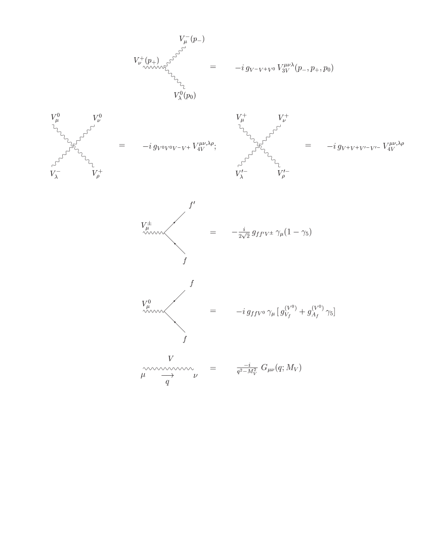
Figure 1: Generic Feynman rules used in our calculation. All kinematic functions and coupling constants are defined in the text.

The Feynman rules used in our calculation are shown in Fig. 1. In these figures, the momenta of the gauge bosons are always defined to be incoming such that the kinematic structures $V_{3V}^{\mu\nu\lambda}$ and $V_{4V}^{\mu\nu,\lambda\rho}$ take the forms:

$$V_{3V}^{\mu\nu\lambda}(p_{-},p_{+},p_{0}) = (p_{-}-p_{+})^{\lambda}\,g^{\mu\nu}+(p_{+}-p_{0})^{\mu}\,g^{\nu\lambda}+(p_{0}-p_{-})^{\nu}\,g^{\mu\lambda}\,,$$ (8)

$$V_{4V}^{\mu\nu,\lambda\rho} = 2g^{\mu\nu}g^{\lambda\rho}-g^{\mu\lambda}g^{\nu\rho}-g^{\mu\rho}g^{\nu\lambda}\,.$$ (9)

Lastly, the massive gauge boson propagator is defined in terms of the kinematic structure $G_{\mu\nu}(q;M_{V})$ which, in unitary gauge, is given by:

$$G_{\mu\nu}(q;M_{V})=g_{\mu\nu}-\frac{q_{\mu}q_{\nu}}{M_{V}^{2}}\,,$$ (10)

where $M_{V}$ is the mass of the propagating gauge boson.

We turn now to the three site Higgsless model which is a prototypical example of the models outlined above.

II.1 The Three Site Higgsless Model

The three site Higgsless model Foadi et al. (2004); Perelstein (2004); Sekhar Chivukula et al. (2006) is a nl$\sigma$m based on the global $SU(2)^{3}\to SU(2)$ symmetry breaking pattern, where the remaining $SU(2)$ plays the role of the custodial symmetry. The gauged sub-group is $SU(2)_{1}\times SU(2)_{2}\times U(1)$ and the symmetry breaking to the SM $SU(2)_{L}\times U(1)_{Y}$ is achieved by two bifundamental $\Sigma$ fields as depicted in the “moose” diagram shown in Fig. 2 .

The nl$\sigma$m fields $\Sigma_{1,2}$ consist of two $SU(2)$ triplets $\pi^{a}_{i}$ ($i=1,2$):

$$\Sigma_{1}=\exp\biggl{[}\frac{2i\pi_{1}^{a}T^{a}}{f_{1}}\biggr{]}\,\,\,\,\,,\,\,\,\,\,\Sigma_{2}=\exp\biggl{[}\frac{2i\pi_{2}^{a}T^{a}}{f_{2}}\biggr{]}\,,$$ (11)

which are coupled to the gauge fields through the covariant derivatives:

$$D_{\mu}\Sigma_{1} = \partial_{\mu}\Sigma_{1}-ig^{\prime}T^{3}B_{\mu}\Sigma_{1}+i\tilde{g}\Sigma_{1}T^{a}W^{a}_{1,\mu}\,,$$ (12)

$$D_{\mu}\Sigma_{2} = \partial_{\mu}\Sigma_{2}-i\tilde{g}T^{a}W^{a}_{1,\mu}\Sigma_{2}+ig\Sigma_{2}T^{a}W^{a}_{2,\mu}\,,$$ (13)

where $g^{\prime}$ is the gauge coupling of the $U(1)$, while $\tilde{g}$ and $g$ are the gauge couplings of $SU(2)_{1}$ and $SU(2)_{2}$, respectively.

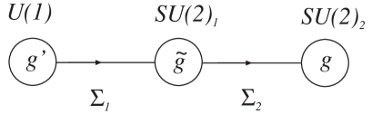
Figure 2: Moose diagram for the three site model (from Ref. Foadi et al. (2004)). The local gauge symmetry $SU(2)_{1}\times SU(2)_{2}\times U(1)$ is gauged as the subgroup of a global $SU(2)^{3}$ symmetry.

The effective Lagrangian for the three site model can be written as an expansion in derivatives (or momenta). At lowest order (dimension-2), the relevant terms which obey the custodial symmetry are:

$${\cal{L}}_{2}=\sum_{i=1}^{2}\frac{f_{i}^{2}}{4}\mbox{Tr}[D^{\mu}\Sigma_{i}(D_{\mu}\Sigma_{i})^{\dagger}]-\frac{1}{4}\sum_{i=1}^{2}W_{i}^{a,\mu\nu}W_{i,\mu\nu}^{a}-\frac{1}{4}B^{\mu\nu}B_{\mu\nu}\,.$$ (14)

In addition to these terms, there is one additional dimension-2 operator which violates the custodial symmetry:

$${\cal{L}}_{2}^{\prime}=\beta_{(2)}\,f_{1}^{2}\,\mbox{Tr}[\Sigma_{1}^{\dagger}(D_{\mu}\Sigma_{1})T^{3}]\,\mbox{Tr}[\Sigma_{1}^{\dagger}(D^{\mu}\Sigma_{1})T^{3}]\,,$$ (15)

as well as dimension-4 operators that respect the symmetries of the theory Chivukula et al. (2007):

$${\cal{L}}_{4} = \alpha_{(1)1}\mbox{Tr}[W_{2,\mu\nu}\Sigma_{2}W_{1}^{\mu\nu}\Sigma_{2}^{\dagger}]+\alpha_{(2)1}\mbox{Tr}[W_{1,\mu\nu}\Sigma_{1}T^{3}B^{\mu\nu}\Sigma_{1}^{\dagger}]$$ (16)

$$-2i\alpha_{(1)2}\mbox{Tr}[(D_{\mu}\Sigma_{2})^{\dagger}(D_{\nu}\Sigma_{2})W_{1}^{\mu\nu}]-2i\alpha_{(2)2}\mbox{Tr}[(D_{\mu}\Sigma_{1})^{\dagger}(D_{\nu}\Sigma_{1})T^{3}B^{\mu\nu}]$$

$$+\sum_{i=1}^{2}\biggl{[}-2i\alpha_{(i)3}\mbox{Tr}[W_{i}^{\mu\nu}(D_{\mu}\Sigma_{i})(D_{\nu}\Sigma_{i})^{\dagger}]+\alpha_{(i)4}\mbox{Tr}[(D_{\mu}\Sigma_{i})(D_{\nu}\Sigma_{i})^{\dagger}]\mbox{Tr}[(D^{\mu}\Sigma_{i})(D^{\nu}\Sigma_{i})^{\dagger}]$$

$$\,\,\,\,\,\,\,\,\,\,\,\,\,\,\,\,\,\,+\alpha_{(i)5}\mbox{Tr}[(D_{\mu}\Sigma_{i})(D^{\mu}\Sigma_{i})^{\dagger}]\mbox{Tr}[(D_{\nu}\Sigma_{i})(D^{\nu}\Sigma_{i})^{\dagger}]\biggr{]}\,.$$

The coefficients of these terms act as counterterms for the divergences which appear at one-loop order and serve to parameterize the effects of unknown high-scale physics Appelquist and Bernard (1980); Longhitano (1980, 1981); Bagger et al. (1993); Perelstein (2004); Chivukula et al. (2007). As we will discuss later, the $\beta_{(2)}$ coefficient contributes to the $T$ parameter while the $\alpha_{(i)1}$ coefficients are relevant to the $S$ parameter.

In unitary gauge ($\Sigma_{1,2}\to 1$), the kinetic energy terms for the $\Sigma$ fields in Eq. (14) only serve to give mass to the various gauge fields. Diagonalizing the resulting charged- and neutral-sector mass matrices, one finds that the spectrum consists of a (massless) photon, relatively light charged and neutral gauge bosons ($W$ and $Z$), as well as heavy charged and neutral gauge bosons ($W^{\prime}$ and $Z^{\prime}$). At this point, there are five free parameters in the model: $g,g^{\prime},\tilde{g},f_{1}$ and $f_{2}$. For the purposes of our calculation, we find it useful to follow Ref. Foadi et al. (2004) and exchange these parameters for the masses of the light VGBs ($M_{W}$ and $M_{Z}$), the masses of the heavy VGBs ($M_{W^{\prime}}$ and $M_{Z^{\prime}}$) and the electromagnetic charge $e$. The latter of which is defined in this model to be:

$$\frac{1}{e^{2}}=\frac{1}{g^{2}}+\frac{1}{\tilde{g}^{2}}+\frac{1}{g^{\prime 2}}\,.$$ (17)

The gauge fields can be expanded in terms of the mass eigenstates. The charged fields can be written as:

$$W_{1}^{\pm} = a_{11}W^{\prime\pm}+a_{12}W^{\pm}\,,$$ (18)

$$W_{2}^{\pm} = a_{21}W^{\prime\pm}+a_{22}W^{\pm}\,,$$ (19)

while the neutral fields are given by:

$$B = b_{00}\gamma+b_{01}Z^{\prime}+b_{02}Z\,,$$ (20)

$$W_{1}^{3} = b_{10}\gamma+b_{11}Z^{\prime}+b_{12}Z\,,$$ (21)

$$W_{2}^{3} = b_{20}\gamma+b_{21}Z^{\prime}+b_{22}Z\,.$$ (22)

Precise formulae for the gauge couplings, the decay constants ($f_{1}$ and $f_{2}$) and the mixing angles ($a_{ij}$ and $b_{ij}$) in terms of the masses of the gauge bosons can be found in Appendix B.

We can now make connection with the generic Feynman rules for the 3- and 4-gauge boson interactions shown in Fig. 1. Inserting Eqs. (18)-(22) into the gauge kinetic terms in Eq. (14), we find that the 3- and 4-point couplings relevant to the calculation of the $S$ and $T$ parameters are given by:

$$g_{W^{-}W^{+}V^{0}_{i}} = g\,a_{22}^{2}\,b_{2i}+\tilde{g}\,a_{12}^{2}\,b_{1i}\,,$$ (23)

$$g_{W^{-}W^{\prime+}V^{0}_{i}} = g\,a_{21}\,a_{22}\,b_{2i}+\tilde{g}\,a_{11}\,a_{12}\,b_{1i}\,,$$ (24)

$$g_{W^{\prime-}W^{\prime+}V^{0}_{i}} = g\,a_{21}^{2}\,b_{2i}+\tilde{g}\,a_{11}^{2}\,b_{1i}\,,$$ (25)

and:

$$g_{V^{0}_{i}V^{0}_{j}W^{-}W^{+}} = g^{2}\,a_{22}^{2}\,b_{2i}\,b_{2j}+\tilde{g}^{2}\,a_{12}^{2}\,b_{1i}\,b_{2j}\,,$$ (26)

$$g_{V^{0}_{i}V^{0}_{j}W^{\prime-}W^{\prime+}} = g^{2}\,a_{21}^{2}\,b_{2i}\,b_{2j}+\tilde{g}^{2}\,a_{11}^{2}\,b_{1i}\,b_{2j}\,,$$ (27)

$$g_{W^{+}W^{\prime+}W^{-}W^{\prime-}} = g^{2}\,a_{21}^{2}\,a_{22}^{2}+\tilde{g}^{2}\,a_{11}^{2}\,a_{12}^{2}\,,$$ (28)

$$g_{W^{+}W^{+}W^{-}W^{-}} = g^{2}\,a_{22}^{4}+\tilde{g}^{2}\,a_{12}^{4}\,,$$ (29)

where ($V^{0}_{0},V^{0}_{1},V^{0}_{2}$) = ($\gamma,Z^{\prime},Z$).

Next, we consider the couplings of the fermions to the gauge fields. In the simplest version of the three site model, the left-handed fermions only couple directly to $SU(2)_{2}$, while the left- and right-handed fermions couple directly to the $U(1)$ with charges $Y_{L}$ and $Y_{R}$, respectively Foadi et al. (2004). In the language of deconstruction, the fermions are localized on the first and third sites. However, it has been shown that this setup leads to an unacceptably large tree-level contribution to the $S$ parameter Foadi et al. (2004); Perelstein (2004); Sekhar Chivukula et al. (2006). A solution to this problem is obtained by allowing the fermions to have a small (but non-zero) coupling to the “middle” $SU(2)$ of Fig. 2 Sekhar Chivukula et al. (2006); Matsuzaki et al. (2006). By appropriately tuning the amount of “delocalization”, one can reduce (or even cancel altogether) the large contribution to the $S$ parameter from the tree level.

The effective Lagrangian describing the coupling of fermions to gauge bosons in the delocalized scenario is then given by:

$${\cal{L}}_{f}=g^{\prime}\,\bar{\psi}\,\gamma_{\mu}(Y_{L}P_{L}+Y_{R}P_{R})B^{\mu}\psi+g\,(1-x_{1})\,\bar{\psi}\,\gamma_{\mu}\,T^{a}W_{2}^{a,\mu}P_{L}\psi+\tilde{g}\,x_{1}\,\bar{\psi}\,\gamma_{\mu}\,T^{a}W_{1}^{a,\mu}P_{L}\psi\,,$$ (30)

where $P_{L,R}$ are projection operators:

$$P_{L,R}=\frac{1}{2}(1\mp\gamma_{5})\,,$$ (31)

and the parameter $x_{1}$ is a measure of the amount of fermion delocalization $(0\leq x_{1}\ll 1)$ Sekhar Chivukula et al. (2006); Matsuzaki et al. (2006). In principle, the value of $x_{1}$ for a given fermion species depends indirectly on the mass of the fermion. This implies that, in general, one should define a different $x_{1}$ for each fermion species. However, since we are only interested in light fermions (i.e., all SM fermions except the top quark), we can safely neglect these differences and assume that the amount of delocalization for all light fermions is the same Matsuzaki et al. (2006).

Expressing the gauge fields in terms of the mass eigenstates using Eqs. (20) and (22), we can identify the couplings and coefficients used in our generic Feynman rules. For example, the couplings for the charged-current interactions are given by:

$$g_{ff^{\prime}W^{\prime\pm}} = g\,(1-x_{1})\,a_{21}+\tilde{g}\,x_{1}\,a_{11}\,,$$ (32)

$$g_{ff^{\prime}W^{\pm}} = g\,(1-x_{1})\,a_{22}+\tilde{g}\,x_{1}\,a_{12}\,.$$ (33)

Next, the expressions for the neutral-current couplings and coefficients can be simplified by making the identification $Y_{R}=Y_{L}+T_{f}^{3}=Q_{f}$. In fact, we find:

$$g_{ffV_{i}^{0}} = g\,(1-x_{1})\,b_{2i}+\tilde{g}\,x_{1}\,b_{1i}-g^{\prime}\,b_{0i}\,,$$ (34)

and:

$$g_{V_{f}}^{(V^{0}_{i})} = \frac{1}{2}T_{f}^{3}+\frac{g^{\prime}b_{0i}}{(g\,(1-x_{1})\,b_{2i}+\tilde{g}\,x_{1}\,b_{1i}-g^{\prime}\,b_{0i})}\,Q_{f}\,,$$ (35)

$$g_{A_{f}}^{(V^{0}_{i})} = -\frac{1}{2}T_{f}^{3}\,.$$ (36)

Having now specified the types of models we are interested in, let us discuss the pinch technique in more detail as well as its application to models with extra dimensions and/or extended gauge symmetries.

III Unitary Gauge and the PT

As mentioned in the Introduction, vector-bosonic loop corrections to the VGB self-energies suffer from two troublesome issues: (i) the final expressions are non-trivially dependent on the particular $R_{\xi}$ gauge used and (ii) use of the unitary gauge ($R_{\xi}\to\infty$) results in non-renormalizable terms. The first issue has been studied in detail in Refs. Degrassi and Sirlin (1992b, a); Papavassiliou and Sirlin (1994); Degrassi et al. (1993). In this paper, we employ the unitary gauge in order to reduce the number of diagrams. Therefore, let us discuss the second issue and its resolution in more detail.

While the unitary gauge is known to result in renormalizable $S$-matrix elements, Green’s functions calculated in this gauge are individually non-renormalizable. These terms are non-renormalizable in the sense that they cannot be removed by the usual mass- and field-renormalization counterterms. To see how this arises, consider the form of the massive VGB propagator in unitary gauge:

$$D_{i}^{\mu\nu}=\frac{-i}{q^{2}-M_{i}^{2}}\biggl{[}g^{\mu\nu}-\frac{q^{\mu}q^{\nu}}{M_{i}^{2}}\biggr{]}\,\,.$$ (37)

The problem arises in the limit $q^{2}\to\infty$ where $D_{i}\sim 1$. In this limit, one-loop amplitudes containing one or more propagators of the form in Eq. (37) become highly divergent. In particular, if dimensional regularization is applied, this divergent behavior manifests itself in poles proportional to higher powers of the external momentum-squared ($q^{2}$) Papavassiliou and Sirlin (1994). For example, two-point functions calculated in unitary gauge contain poles proportional to $q^{4}$ and $q^{6}$.

The Pinch Technique supplies a solution to both the gauge-dependence and the appearance of the $q^{4}$ and $q^{6}$ terms via a systematic algorithm which leads to the rearrangement of one-loop Feynman graphs contributing to a gauge-invariant and renormalizable amplitude Cornwall (1981, 1982); Cornwall and Papavassiliou (1989); Papavassiliou (1990). The end results of the rearrangement are individually gauge-independent propagator-, vertex- and box-like structures which are void of any higher powers of $q^{2}$. In other words, propagator-like or “pinch” terms coming from vertex and box corrections are isolated in a systematic manner and added to the self-energies. These pinch pieces carry the exact gauge-dependent and non-renormalizable terms needed to cancel those of the two-point functions. Finally, to construct gauge-invariant expressions for the oblique parameters at one-loop, one needs only replace the various $\Pi_{ij}$ calculated from two-point diagrams with their PT counterparts, $\Pi_{ij}^{\mbox{\tiny PT}}$ Degrassi et al. (1993). In the following sections, we will demonstrate how to construct the PT self-energies in models with additional, massive gauge bosons.

Figure 3: Schematic example of the extraction of pinch pieces from vertex corrections.

Before moving on to our results, though, let us first give a simple example of how the pinch terms are isolated. Consider the vertex diagram shown on the left side of Fig. 3 where the external and internal fermions are considered to be massless. When the $W$ propagator (with loop momentum $k$) is contracted with the $Wff^{\prime}$ vertex, a term arises of the form:

$${\cal{A}}_{V}^{\mu} \sim \int\frac{d^{n}k}{(2\pi)^{n}}\bar{u}(p_{2})\biggl{\{}\cdots(\not{k}+\not{p_{1}})\not{k}\cdots\biggr{\}}u(p_{1})\frac{1}{(k^{2}-M_{W}^{2})(k+p_{1})^{2}(k-q)^{2}}$$ (38)

$$= \int\frac{d^{n}k}{(2\pi)^{n}}\bar{u}(p_{2})\biggl{\{}\cdots(\not{k}+\not{p_{1}})((\not{k}+\not{p_{1}})-\not{p_{1}})\cdots\biggr{\}}u(p_{1})\frac{1}{(k^{2}-M_{W}^{2})(k+p_{1})^{2}(k-q)^{2}}$$

$$= \int\frac{d^{n}k}{(2\pi)^{n}}\bar{u}(p_{2})\biggl{\{}\cdots(k+p_{1})^{2}\cdots\biggr{\}}u(p_{1})\frac{1}{(k^{2}-M_{W}^{2})(k+p_{1})^{2}(k-q)^{2}}+\cdots\,\,.$$

In the second line, we have written the second factor of ${\not k}$ in terms of adjacent, inverse fermion propagators. Canceling the factor of $(k+p_{1})^{2}$ in the numerator and denominator, we see that the first term in the third line resembles a correction to the $W$ propagator, i.e. it is propagator-like, and can be represented schematically as shown on the right side of Fig. 3. This pinch term (along with others coming from other vertex and box corrections) is then combined with the loop-corrected two-point function to construct the self-energy for the $W$ boson.

IV One-loop Corrections to the Neutral Currents

In this section, we outline the calculation of the one-loop corrections needed to construct the self-energies for the neutral gauge bosons using the Pinch Technique Degrassi and Sirlin (1992b, a). We write all amplitudes in terms of the generic couplings defined in Fig. 1 and reduce all tensor integrals to the usual Passarino-Veltman (P-V) tensor integral coefficients Passarino and Veltman (1979) and scalar integrals defined in Appendix  A.

The PT self-energies for the neutral VGBs are calculated in the context of four-fermion scattering, in particular $\ell^{-}\ell^{+}\to\ell^{-}\ell^{+}$, with all external (and internal) fermions considered to be massless . The one-loop corrections are shown schematically in Fig. 4. In the following, we calculate the corrections to the gauge boson propagators, as well as the pinch pieces from both vertex and box corrections.

Figure 4: One-loop corrections to $t$-channel $\ell^{-}\ell^{+}$ scattering. From left to right, the corrections consist of one-loop corrections to the gauge boson propagator, corrections to the $V^{0}\ell\ell$ vertices and box corrections.

IV.1 Corrections to the Gauge Boson Propagators

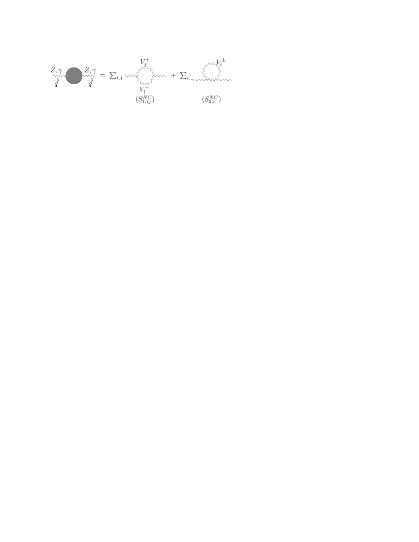
Figure 5: General corrections to the two-point functions of the neutral gauge bosons.

The one-loop corrections to the neutral gauge boson propagators are shown in Fig. 5. In terms of the amplitudes of these diagrams, the transverse two-point functions for the SM neutral gauge bosons can be constructed as:

$$i\Pi_{mn}(q^{2})\,g^{\mu\nu}=i\biggl{[}\sum_{i,j}S_{1,ij}^{NC,\mu\nu}+\sum_{i}S_{2,i}^{NC,\mu\nu}\biggr{]}\,,$$ (39)

where $(mn)=(\gamma\gamma),(ZZ)$ or $(Z\gamma)$. The structures of the individual amplitudes take the forms:

$$S_{1,ij}^{NC,\mu\nu} = g_{V^{-}_{i}V^{+}_{j}\gamma(Z)}^{2}\biggl{[}C_{S}^{(0)}+C_{S}^{(2)}\,q^{2}+C_{S}^{(4)}\,q^{4}\biggr{]}g^{\mu\nu}\,,$$ (40)

$$S_{2}^{NC,\mu\nu} = g_{\gamma\gamma(ZZ)V^{-}_{i}V^{+}_{i}}\biggl{[}-\frac{9}{2}+\frac{15}{4}\epsilon\biggr{]}\,A_{0}(M_{i})\,g^{\mu\nu}\,,$$ (41)

where:

$$C_{S}^{(0)} = \biggl{(}10+\frac{M_{i}^{2}}{M_{j}^{2}}+\frac{M_{j}^{2}}{M_{i}^{2}}-8\epsilon\biggr{)}\,B_{22}(q^{2};M_{i},M_{j})+\biggl{(}M_{i}^{2}+M_{j}^{2}-\frac{M_{i}^{4}}{M_{j}^{2}}-\frac{M_{j}^{4}}{M_{i}^{2}}\biggr{)}B_{0}(q^{2};M_{i},M_{j})$$ (42)

$$\,\,\,\,\,\,\,\,+\biggl{(}\frac{1}{4}-\frac{M_{j}^{2}}{M_{i}^{2}}+\frac{\epsilon}{8}\biggr{)}A_{0}(M_{i})+\biggl{(}\frac{1}{4}-\frac{M_{i}^{2}}{M_{j}^{2}}+\frac{\epsilon}{8}\biggr{)}A_{0}(M_{j})\,,$$

$$C_{S}^{(2)} = -2\biggl{(}\frac{1}{M_{i}^{2}}+\frac{1}{M_{j}^{2}}\biggr{)}B_{22}(q^{2};M_{i},M_{j})+2\biggl{(}2+\frac{M_{i}^{2}}{M_{j}^{2}}+\frac{M_{j}^{2}}{M_{i}^{2}}\biggr{)}B_{0}(q^{2};M_{i},M_{j})$$ (43)

$$\,\,\,\,\,\,\,\,+\frac{1}{M_{i}^{2}}A_{0}(M_{i})+\frac{1}{M_{j}^{2}}A_{0}(M_{j})\,,$$

$$C_{S}^{(4)} = \frac{1}{M_{i}^{2}M_{j}^{2}}\biggl{[}B_{22}(q^{2};M_{i},M_{j})-(M_{i}^{2}+M_{j}^{2})B_{0}(q^{2};M_{i},M_{j})\biggr{]}\,.$$ (44)

In the above and the following, $A_{0}$ and $B_{0}$ represent the one- and two-point scalar integrals, respectively, while the $B_{ij}$’s represent the P-V tensor integral coefficients Passarino and Veltman (1979) (see Appendix A).

IV.2 Pinch Contributions from Vertex Corrections

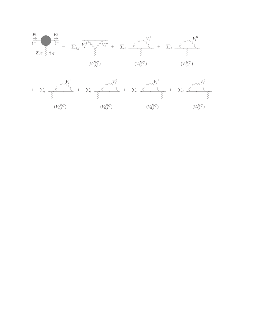
Figure 6: General one-loop corrections to the neutral gauge-boson-fermion vertices and the external legs which give rise to pinch contributions.

The one-loop vertex corrections for the neutral current are shown in Fig. 6. Note that we have included the external leg corrections in addition to the traditional vertex corrections. In Appendix C, we discuss additional corrections which can arise due to mixing between the light and heavy gauge bosons at the one-loop level. When the mass of the heavy gauge boson is much larger than $q^{2}$, the corrections from these mixings become “pinch-like” and should be combined with the corrections from vertices and boxes. The pinch contributions to the total amplitude from vertex corrections take the form:

$$\Delta{\cal{A}}_{V,\gamma(Z)}^{\mu}|_{pinch} = \{V_{\gamma(Z)}\}\,[\bar{u}(p_{i})\,\gamma^{\mu}(1-\gamma_{5})\,u(p_{i})]$$ (45)

$$\equiv \{V_{\gamma(Z)}\}\,\Gamma_{W}^{\mu}\,,$$

where $\{V_{\gamma(Z)}\}$ represents the sum of the pinch contributions calculated from the diagrams shown in Fig. 6 and $\Gamma_{W}$ is the current associated with the SM-like $W$. In applying the PT to the neutral currents, we find it useful to rewrite $\Gamma_{W}$ in terms of the currents associated with the SM-like $Z$ and photon. For example, using Eqs. (34)-(36), this structure in the three site model can be rewritten as:

$$\Gamma_{W}^{\mu}\equiv\bar{u}(p_{j})\gamma^{\mu}(1-\gamma_{5})u(p_{i}) = \frac{2}{T^{3}_{f}}\,\bar{u}(p_{j})\,\gamma^{\mu}\biggl{[}\biggl{(}\frac{1}{2}T^{3}_{f}+\frac{g^{\prime}\,b_{02}}{(g\,(1-x_{1})\,b_{22}+\tilde{g}\,x_{1}\,b_{12}-g^{\prime}\,b_{02})}\,Q_{f}\biggr{)}$$ (46)

$$\,\,\,\,\,\,\,\,\,\,-\frac{g^{\prime}\,b_{02}}{(g\,(1-x_{1})\,b_{22}+\tilde{g}\,x_{1}\,b_{12}-g^{\prime}\,b_{02})}\,Q_{f}-\frac{1}{2}T^{3}_{f}\,\gamma_{5}\biggr{]}\,u(p_{i})$$

$$= \frac{2}{T^{3}_{f}}\,\bar{u}(p_{j})\,\gamma^{\mu}\biggl{[}(g_{V_{f}}^{(Z)}+g_{A_{f}}^{(Z)}\,\gamma_{5})$$

$$\,\,\,\,\,\,\,\,\,\,+\frac{g^{\prime}\,b_{02}}{(g\,(1-x_{1})\,b_{22}+\tilde{g}\,x_{1}\,b_{12}-g^{\prime}\,b_{02})}\,Q_{f}\biggl{]}\,u(p_{i})$$

$$\equiv \frac{2}{T^{3}_{f}}\biggl{[}\Gamma_{Z}^{\mu}+\frac{g^{\prime}\,b_{02}}{(g\,(1-x_{1})\,b_{22}+\tilde{g}\,x_{1}\,b_{12}-g^{\prime}\,b_{02})}\,Q_{f}\,\Gamma_{\gamma}^{\mu}\biggr{]}\,,$$

where we have defined the currents associated with the SM $Z$ and photon respectively as:

$$\Gamma_{Z}^{\mu} = \bar{u}(p_{j})\,\gamma^{\mu}(g_{V_{f}}^{(Z)}+g_{A_{f}}^{(Z)}\gamma_{5})\,u(p_{i})\,,$$ (47)

$$\Gamma_{\gamma}^{\mu} = \bar{u}(p_{j})\,\gamma^{\mu}\,u(p_{i})\,.$$ (48)

Using the Feynman rules defined in Fig. 1 and reducing all amplitudes to P-V tensor coefficients and scalar integrals, we find that the pinch pieces from the individual diagrams shown in Fig. 6 are given by:

$$\{V_{1,ij}^{NC}\} = -g_{\ell\nu V_{i}^{\pm}}\,g_{\ell\nu V_{j}^{\pm}}\,g_{\gamma(Z)V^{+}_{j}V^{-}_{i}}\,\,[\,C_{V}^{(0)}+C_{V}^{(2)}\,q^{2}\,]$$ (49)

$$\{V_{2,i}^{NC}\} = -g^{2}_{\ell\nu V_{i}^{\pm}}\,g_{\nu\nu\gamma(Z)}\,\,[g_{V_{\nu}}^{(\gamma,Z)}-g_{A_{\nu}}^{(\gamma,Z)}]\,\,\frac{A_{0}(M_{i})}{M_{i}^{2}}$$ (50)

$$\{V_{3,i}^{NC}\}^{\mu} = g^{2}_{\ell\ell V_{i}^{0}}\,g_{\ell\ell\gamma(Z)}\,\,\frac{A_{0}(M_{i})}{M_{i}^{2}}\,\bar{u}(p_{2})\,\gamma^{\mu}\biggl{[}(2g_{V_{\ell}}^{(V^{0})}g_{A_{\ell}}^{(V^{0})}g_{A_{\ell}}^{(\gamma,Z)}+(g_{V_{\ell}}^{(V^{0})})^{2}g_{V_{\ell}}^{(\gamma,Z)}+(g_{A_{\ell}}^{(V^{0})})^{2}g_{V_{\ell}}^{(\gamma,Z)})$$ (51)

$$+\gamma_{5}(2g_{V_{\ell}}^{(V^{0})}g_{A_{\ell}}^{(V^{0})}g_{V_{\ell}}^{(\gamma,Z)}+(g_{V_{\ell}}^{(V^{0})})^{2}g_{A_{\ell}}^{(\gamma,Z)}+(g_{A_{\ell}}^{(V^{0})})^{2}g_{A_{\ell}}^{(\gamma,Z)})\biggr{]}u(p_{1})$$

$$\{V_{4,i}^{NC}\} = \frac{g_{\ell\nu V_{i}^{\pm}}^{2}\,g_{\ell\ell\gamma(Z)}}{2}\,(g_{V_{\ell}}^{(\gamma,Z)}-g_{A_{\ell}}^{(\gamma,Z)})\frac{A_{0}(M_{i})}{M_{i}^{2}}$$ (52)

$$\{V_{5,i}^{NC}\}^{\mu} = -\frac{1}{2}\{V_{3,i}^{NC}\}^{\mu}$$ (53)

$$\{V_{6,i}^{NC}\} = \{V_{4,i}^{NC}\}$$ (54)

$$\{V_{7,i}^{NC}\}^{\mu} = \{V_{5,i}^{NC}\}^{\mu}=-\frac{1}{2}\{V_{3,i}^{NC,\mu}\}\,,$$ (55)

where:

$$C_{V}^{(0)} = \biggl{(}-3+2\epsilon\biggr{)}\biggl{(}\frac{1}{M_{i}^{2}}+\frac{1}{M_{j}^{2}}\biggr{)}B_{22}(q^{2};M_{i},M_{j})+2B_{0}(q^{2},M_{i},M_{j})$$ (56)

$$C_{V}^{(2)} = \biggl{[}\frac{1}{M_{j}^{2}}B_{0}(q^{2};M_{i},M_{j})-\frac{2}{M_{i}^{2}}B_{11}(q^{2};M_{i},M_{j})-\biggl{(}\frac{1}{M_{i}^{2}}+\frac{1}{M_{j}^{2}}\biggr{)}B_{21}(q^{2};M_{i},M_{j})$$ (57)

$$\,\,\,\,\,\,\,\,-\frac{1}{M_{i}^{2}M_{j}^{2}}B_{22}(q^{2};M_{i},M_{j})\biggr{]}\,.$$

Thus, we immediately see that the pinch pieces from the vertex corrections and external leg corrections containing a virtual, neutral gauge boson ($V^{0}$) cancel amongst themselves, i.e.:

$$\{V_{3,i}^{NC}\}^{\mu}+\{V_{5,i}^{NC}\}^{\mu}+\{V_{7,i}^{NC}\}^{\mu}=0\,.$$ (58)

Note that this is true regardless of the exact form of the couplings. Finally, in terms of the above amplitudes, the total pinch contribution from the vertex corrections is given by:

$$\{V_{\gamma(Z)}\}=\sum_{i,j}\{V_{1,ij}^{NC}\}+\sum_{i}\biggl{[}\{V_{2,i}^{NC}\}+\{V_{4,i}^{NC}\}+\{V_{6,i}^{NC}\}\biggr{]}\,.$$ (59)

IV.3 Pinch Contributions from Box Corrections

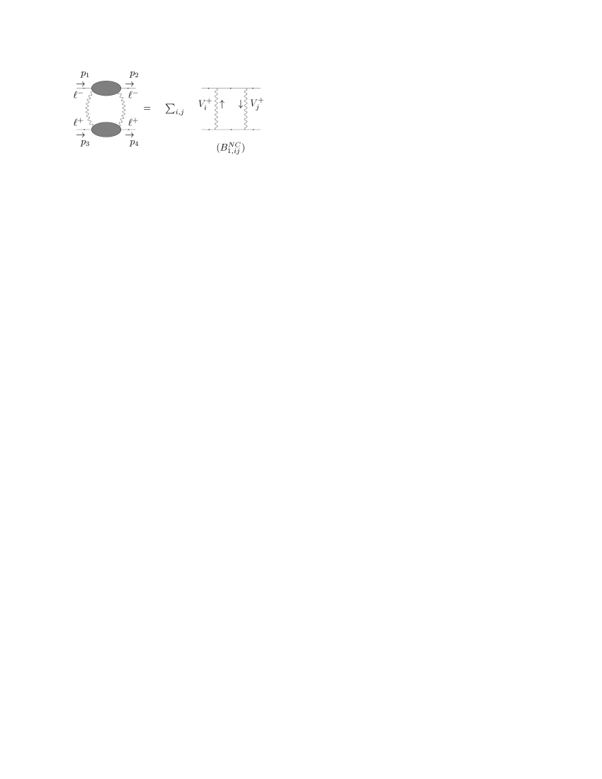
Figure 7: General one-loop box corrections from charged VGBs which contain pinch contributions.

The one-loop box diagrams which give rise to pinch contributions are depicted in Fig. 7. The total pinch amplitude arising from these corrections can be written as:

$$\Delta{\cal{A}}_{B,\gamma(Z)}^{\mu}|_{pinch}=\{B_{\gamma(Z)}\}\,\Gamma_{W}^{\mu}\,\Gamma_{W,\mu}\,,$$ (60)

where $\{B_{\gamma(Z)}\}$ represents the sum of the pinch contributions from the box diagrams. Individually, the amplitudes for these diagrams take the compact form:

$$\{B_{1,ij}^{NC}\} = \frac{g_{\ell\nu V_{i}^{\pm}}^{2}g_{\ell\nu V_{j}^{\pm}}^{2}}{M_{i}^{2}M_{j}^{2}}\biggl{[}B_{22}(q^{2};M_{i},M_{j})-(M_{i}^{2}+M_{j}^{2})B_{0}(q^{2};M_{i},M_{j})\biggr{]}\,.$$ (61)

such that the total pinch contributions from box corrections $\{B_{1,ij}^{NC}\}$ is given by:

$$\{B_{\gamma(Z)}\}=\sum_{i,j}\{B_{1,ij}^{NC}\}\,.$$ (62)

V One-Loop Corrections to the Charged Current

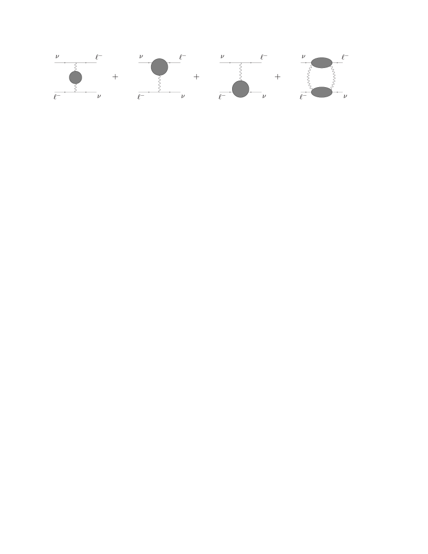
Figure 8: Schematic depiction of the one-loop corrections to $t$-channel $\nu\ell^{-}$ scattering.

In this section, we calculate the one-loop corrections needed to construct the $W$ boson self-energy using the PT Papavassiliou and Sirlin (1994). The loop-corrected amplitudes are again calculated in the context of four-fermion scattering. In particular, we consider the one-loop corrections to $\nu\ell^{-}\to\nu\ell^{-}$ which are schematically depicted in Fig. 8.

V.1 Corrections to the $W$ Boson Propagator

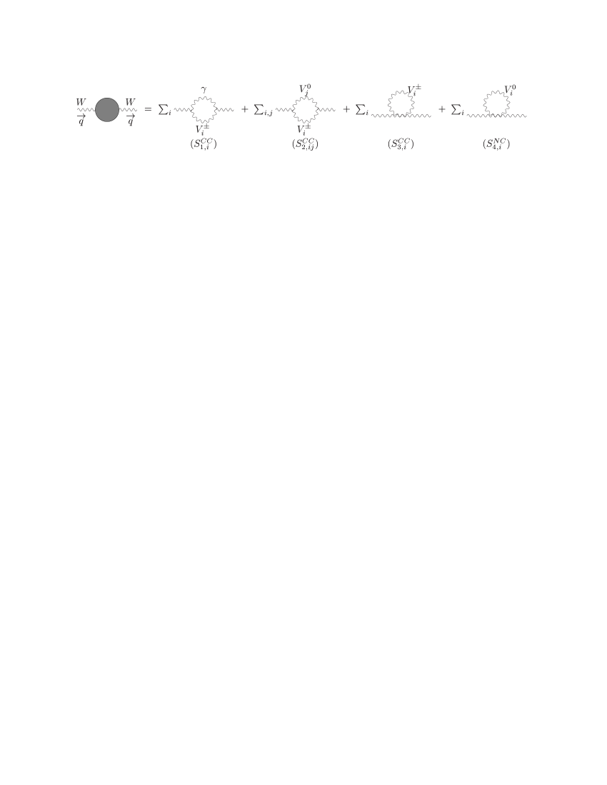
Figure 9: General corrections to the two-point functions of the $W$ gauge boson.

The one-loop corrections to the $W$ boson propagator are shown in Fig. 9. In terms of these diagrams, the transverse two-point function of the $W$ boson is:

$$i\Pi_{WW}(q^{2})g^{\mu\nu}=i\biggl{[}\sum_{i}S_{1,i}^{CC,\mu\nu}+\sum_{i,j}S_{2,ij}^{CC,\mu\nu}+\sum_{i}S_{3,i}^{CC,\mu\nu}+\sum_{i}S_{4,i}^{CC,\mu\nu}\biggr{]}\,.$$ (63)

Note that we have distinguished the photon from the other neutral gauge bosons in Fig. 9. Since the photon is massless, the kinematic structures of these diagrams are slightly different than those for massive, neutral gauge bosons. The amplitudes for all of these diagrams take compact forms:

$$S_{1,i}^{CC,\mu\nu} = g_{W^{-}V_{i}^{+}\gamma}^{2}\biggl{[}K_{S}^{(0)}+K_{S}^{(2)}\,q^{2}+K_{S}^{(4)}\,q^{4}\biggr{]}\,g^{\mu\nu}\,,$$ (64)

$$S_{2,ij}^{CC,\mu\nu} = g_{W^{-}V_{i}^{+}V_{j}^{0}}^{2}\biggl{[}C_{S}^{(0)}+C_{S}^{(2)}\,q^{2}+C_{S}^{(4)}\,q^{4}\biggr{]}\,g^{\mu\nu}\,,$$ (65)

$$S_{3,i}^{CC,\mu\nu} = g_{W^{+}V_{i}^{+}W^{-}V_{i}^{-}}\biggl{[}-\frac{9}{4}+\frac{15}{8}\epsilon\biggr{]}\,A_{0}(M_{i})\,g^{\mu\nu}\,,$$ (66)

$$S_{4,i}^{CC,\mu\nu} = g_{V_{i}^{0}V_{i}^{0}W^{-}W^{+}}\biggl{[}-\frac{9}{4}+\frac{15}{8}\epsilon\biggr{]}\,A_{0}(M_{i})\,g^{\mu\nu}\,,$$ (67)

where the $C_{S}^{(i)}$ coefficients are the same as those in Eqs. (42)-(44) and the $K_{S}^{(i)}$ coefficients are given by:

$$K_{S}^{(0)} = (10-8\epsilon)B_{22}(q^{2};M_{i},0)+M_{i}^{2}B_{0}(q^{2};M_{i},0)+\biggl{(}\frac{1}{4}+\frac{\epsilon}{8}\biggr{)}A_{0}(M_{i})\,,$$ (68)

$$K_{S}^{(2)} = -\frac{2}{M_{i}^{2}}B_{22}(q^{2};M_{i},0)+4B_{0}(q^{2};M_{i},0)+\frac{A_{0}(M_{i})}{M_{i}^{2}}\,,$$ (69)

$$K_{S}^{(4)} = -\frac{1}{M_{i}^{2}}B_{0}(q^{2};M_{i},0)\,.$$ (70)

V.2 Pinch Contributions from Vertex Corrections

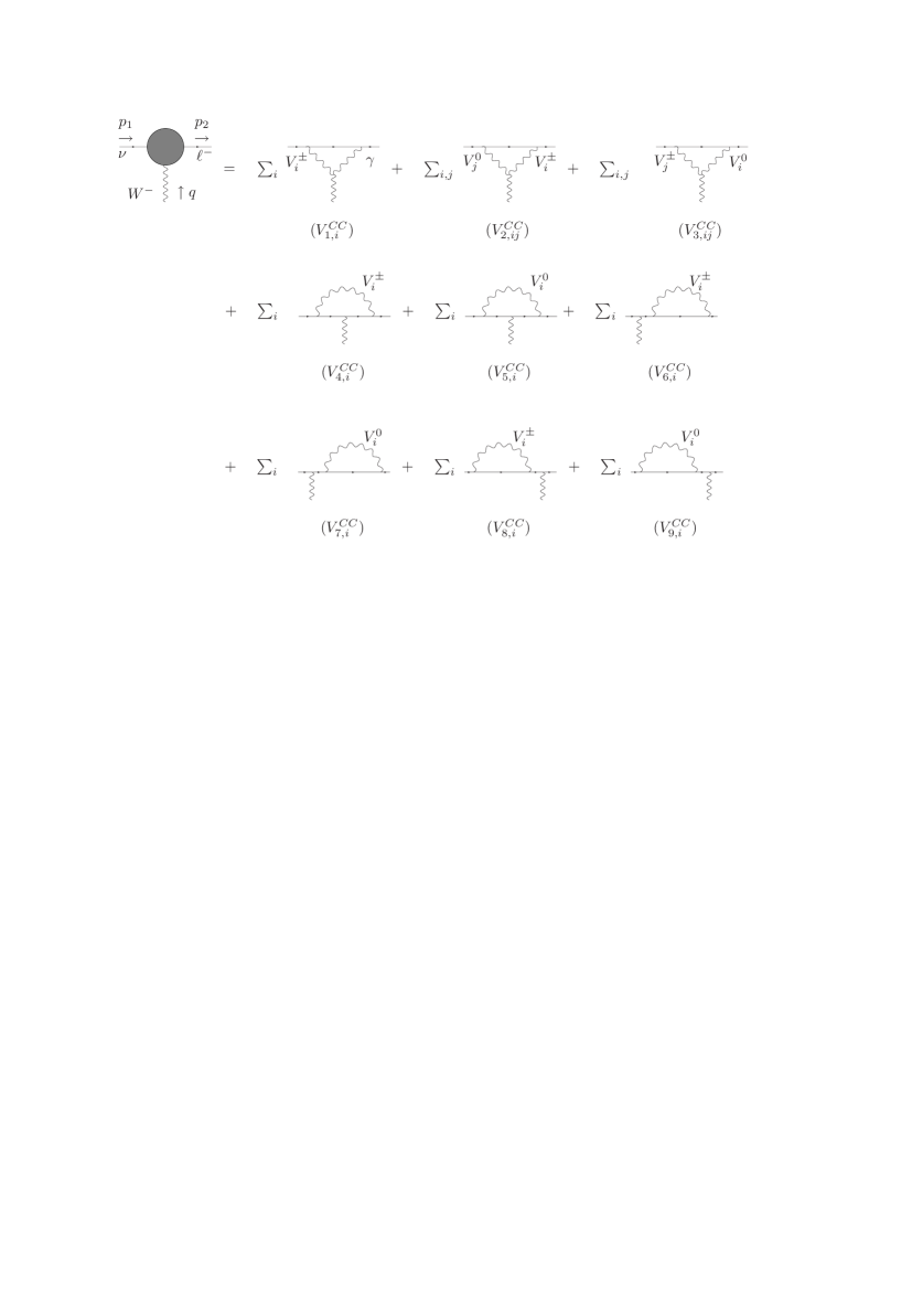
Figure 10: General one-loop corrections to the gauge-boson-fermion vertices and external fermion legs which give rise to pinch contributions.

The one-loop vertex corrections which give rise to pinch contributions are shown in Fig. 10 . The amplitude structure of the vertex diagrams is very similar to the neutral current amplitudes with the exception of diagrams $(V_{1,i}^{CC})$ and $(V_{2,i}^{CC})$. The pinch contributions from the vertex corrections take the form:

$$\Delta{\cal{A}}_{V,W}^{\mu}|_{pinch}=\{V_{W}\}\,\Gamma_{W}^{\mu}\,,$$ (71)

where $\{V_{W}\}$ is the sum of the pinch contributions from the diagrams in Fig. 10 and $\Gamma_{W}$ is defined in Eq. (45). The individual amplitudes which contribute to $\{V_{W}\}$ can be written as:

$$\{V_{1,i}^{CC}\} = \frac{g_{\ell\nu V_{i}^{\pm}}\,g_{\ell\ell\gamma}\,g_{W^{-}V_{i}^{+}\gamma}}{2\sqrt{2}}\,\,(g_{V_{\ell}}^{(\gamma)}-g_{A_{\ell}}^{(\gamma)})\,[\,K_{V}^{(0)}+K_{V}^{(2)}\,q^{2}\,]\,,$$ (72)

$$\{V_{2,ij}^{CC}\} = -\frac{g_{\ell\nu V_{i}^{\pm}}\,g_{\nu\nu V_{j}^{0}}\,g_{W^{-}V_{i}^{+}V_{j}^{0}}}{2\sqrt{2}}\,\,(g_{V_{\nu}}^{(V^{0})}-g_{A_{\nu}}^{(V^{0})})\,[\,C_{V}^{(0)}+C_{V}^{(2)}\,q^{2}\,]\,,$$ (73)

$$\{V_{3,ij}^{CC}\} = \frac{g_{\ell\nu V_{j}^{\pm}}\,g_{\ell\ell V_{i}^{0}}\,g_{W^{-}V_{j}^{+}V_{i}^{0}}}{2\sqrt{2}}\,\,(g_{V_{\ell}}^{(V^{0})}-g_{A_{\ell}}^{(V^{0})})\,[\,C_{V}^{(0)}+C_{V}^{(2)}\,q^{2}\,]\,,$$ (74)

$$\{V_{4,i}^{CC}\} = \frac{g_{\ell\nu V_{i}^{\pm}}^{2}g_{\ell\nu W^{\pm}}}{2\sqrt{2}}\biggl{(}\frac{1}{2}\biggr{)}\,\frac{A_{0}(M_{i})}{M_{i}^{2}}\,,$$ (75)

$$\{V_{5,i}^{CC}\} = \frac{g_{\nu\nu V_{i}^{0}}g_{\ell\ell V_{i}^{0}}g_{\ell\nu W^{\pm}}}{2\sqrt{2}}(g_{V_{\ell}}^{(V^{0})}-g_{A_{\ell}}^{(V^{0})})(g_{V_{\nu}}^{(V^{0})}-g_{A_{\nu}}^{(V^{0})})\,\frac{A_{0}(M_{i})}{M_{i}^{2}}\,,$$ (76)

$$\{V_{6,i}^{CC}\} = -\{V_{4,i}^{CC}\}\,,$$ (77)

$$\{V_{7,i}^{CC}\} = -\frac{g_{\ell\ell V^{0}}^{2}g_{\ell\nu W^{\pm}}}{2\sqrt{2}}\biggl{(}\frac{1}{2}\biggr{)}(g_{V_{\ell}}^{(V^{0})}-g_{A_{\ell}}^{(V^{0})})^{2}\,\frac{A_{0}(M_{i})}{M_{i}^{2}}\,,$$ (78)

$$\{V_{8,i}^{CC}\} = \{V_{6,i}^{CC}\}=-\{V_{4,i}^{CC}\}\,,$$ (79)

$$\{V_{9,i}^{CC}\} = -\frac{g_{\nu\nu V^{0}}^{2}g_{\ell\nu W^{\pm}}}{2\sqrt{2}}\biggl{(}\frac{1}{2}\biggr{)}(g_{V_{\nu}}^{(V^{0})}-g_{A_{\nu}}^{(V^{0})})^{2}\,\frac{A_{0}(M_{i})}{M_{i}^{2}}\,,$$ (80)

where the $C_{V}^{(i)}$ coefficients are given by Eqs. (56) and (57) and the $K_{V}^{(i)}$ coefficients are given by:

$$K_{V}^{(0)} = \frac{1}{M_{i}^{2}}(-3+2\epsilon)B_{22}(q^{2};M_{i},0)+2B_{0}(q^{2};M_{i},0)\,,$$ (81)

$$K_{V}^{(2)} = \frac{1}{M_{i}^{2}}\biggl{[}B_{0}(q^{2};0,M_{i})-B_{21}(q^{2};0,M_{i})\biggr{]}\,.$$ (82)

Finally, the total pinch contribution from the vertex corrections can then be calculated by summing the above amplitudes:

$$\{V_{W}\} = \sum_{i}\biggl{[}\{V_{1,i}^{CC}\}+\{V_{4,i}^{CC}\}+\{V_{5,i}^{CC}\}+\{V_{6,i}^{CC}\}+\{V_{7,i}^{CC}\}+\{V_{8,i}^{CC}\}+\{V_{9,i}^{CC}\}\biggr{]}$$ (83)

$$+\sum_{i,j}\biggl{[}\{V_{2,ij}^{CC}\}+\{V_{3,ij}^{CC}\}\biggr{]}\,.$$

V.3 Pinch Contributions from Box Corrections

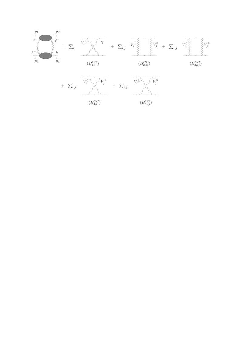
Figure 11: General one-loop box corrections to the charged current process.

The one-loop box corrections which contribute to the $W$ boson PT self-energy are shown in Fig 11. Extracting the pinch contributions, the amplitude from box corrections takes the form:

$$\Delta{\cal{A}}_{B,W}^{\mu}|_{pinch}=\{B_{W}\}\,\Gamma_{W}^{\mu}\,\Gamma_{W,\mu}\,,$$ (84)

where $\{B_{W}\}$ represents the pinch piece of the total box amplitude. Since the photon only couples to charged fermions, there is only one diagram involving a photon which gives a non-zero contribution to the total pinch amplitude:

$$\{B_{1,i}^{CC}\} = -\frac{g_{\ell\ell\gamma}^{2}g_{\ell\nu V_{i}^{\pm}}^{2}}{(2\sqrt{2})^{2}}\frac{(g_{V_{\ell}}^{(\gamma)}-g_{A_{\ell}}^{(\gamma)})^{2}}{M_{i}^{2}}\,B_{0}(q^{2};M_{i},0)\,.$$ (85)

The other four diagrams, those which contain a massive neutral gauge boson as well as a massive charged gauge boson, have kinematic structures identical to $\{B_{1,i}^{NC}\}$ (Eq. (61)). In fact, we find:

$$\{B_{2,ij}^{CC}\} = -\frac{g_{\ell\ell V_{j}^{0}}g_{\nu\nu V_{j}^{0}}g_{\ell\nu V_{i}^{\pm}ff}^{2}}{(2\sqrt{2})^{2}}\frac{(g_{V_{\ell}}^{(V^{0})}-g_{A_{\ell}}^{(V^{0})})(g_{V_{\nu}}^{(V^{0})}-g_{A_{\nu}}^{(V^{0})})}{M_{i}^{2}M_{j}^{2}}$$ (86)

$$\,\,\,\,\,\,\,\,\,\,\,\times\biggl{[}B_{22}(q^{2};M_{i},M_{j})-(M_{i}^{2}+M_{j}^{2})B_{0}(q^{2};M_{i},M_{j})\biggr{]}\,,$$

$$\{B_{3,ij}^{CC}\} = \{B_{2,ij}^{NC}\}\,\,\,\,\,\,\,\,\mbox{(with $i\leftrightarrow j$)}\,,$$ (87)

$$\{B_{4,ij}^{CC}\} = -\frac{g_{\nu\nu V_{i}^{0}}^{2}g_{\ell\nu V_{j}^{\pm}}^{2}}{(2\sqrt{2})^{2}}\frac{(g_{V_{\nu}}^{(V^{0})}-g_{A_{\nu}}^{(V^{0})})^{2}}{M_{i}^{2}M_{j}^{2}}$$ (88)

$$\,\,\,\,\,\,\,\,\,\,\,\times\biggl{[}B_{22}(q^{2};M_{i},M_{j})-(M_{i}^{2}+M_{j}^{2})B_{0}(q^{2};M_{i},M_{j})\biggr{]}\,,$$

$$\{B_{5,ij}^{CC}\} = -\frac{g_{\ell\ell V_{i}^{0}}^{2}g_{\ell\nu V_{j}^{\pm}}^{2}}{(2\sqrt{2})^{2}}\frac{(g_{V_{\ell}}^{(V^{0})}-g_{A_{\ell}}^{(V^{0})})^{2}}{M_{i}^{2}M_{j}^{2}}$$ (89)

$$\,\,\,\,\,\,\,\,\,\,\,\times\biggl{[}B_{22}(q^{2};M_{i},M_{j})-(M_{i}^{2}+M_{j}^{2})B_{0}(q^{2};M_{i},M_{j})\biggr{]}\,.$$

Finally, in terms of these amplitudes, the total pinch contribution from box corrections is given by:

$$\{B_{W}\} = \sum_{i}\,\{B_{1,ij}^{CC}\}+\sum_{i,j}\biggl{[}\{B_{2,ij}^{CC}\}+\{B_{3,ij}^{CC}\}+\{B_{4,ij}^{CC}\}+\{B_{5,ij}^{CC}\}\biggr{]}\,.$$ (90)

VI The Gauge Boson Self-energies in the PT

In this section, we demonstrate how to construct the self-energies for the SM-like gauge bosons using the various pieces calculated in the previous sections. We will do this first for a general model and then, in the next section, apply our results to the three site model. As stated earlier, we consider the process $\ell^{-}(p_{1})+\ell^{+}(p_{3})\to\ell^{-}(p_{2})+\ell^{+}(p_{4})$ for the neutral currents and the process $\nu(p_{1})+\ell^{-}(p_{3})\to\ell^{-}(p_{2})+\nu(p_{4})$ for the charged current where both the neutral and charged gauge bosons are exchanged in the $t$-channel as depicted in Figs. 4 and 8 respectively. The results given below, however, are independent of the particular process Degrassi and Sirlin (1992a).

VI.1 The Neutral Gauge Boson Self-energies

Let us begin by constructing the the PT self-energy for the photon. The tree-level amplitude for the $t$-channel exchange of a photon is given by:

$$A^{0}_{\gamma}\equiv-\frac{i\,e^{2}}{q^{2}}\,\Gamma_{\gamma}^{\mu}\,\Gamma_{\gamma,\mu}\,.$$ (91)

where we have made use of Eq. (7). The amplitude from the loop-corrected photon propagator diagrams takes the form :

$$A^{S}_{\gamma}=\biggl{(}-\frac{i\,e^{2}}{q^{2}}\,\Gamma_{\gamma}^{\mu}\,\Gamma_{\gamma,\mu}\biggr{)}\,\frac{\Pi_{\gamma\gamma}}{q^{2}}\equiv A^{0}_{\gamma}\,\frac{\Pi_{\gamma\gamma}}{q^{2}}\,,$$ (92)

where $\Pi_{\gamma\gamma}$ represents the sum of the diagrams contributing to the photon’s two-point function as given by Eq. (39).

Next, we consider the pinch pieces coming from the $\gamma\ell\ell$ vertex corrections. In this case, we sum the two middle diagrams of Fig. 4 to find:

$$A^{V}_{\gamma}=2\,\biggl{(}-\frac{i\,e^{2}}{q^{2}}\,\Gamma_{\gamma}^{\mu}\,\Gamma_{\gamma,\mu}\biggr{)}\,\{V_{\gamma}\}\equiv 2\,A^{0}_{\gamma}\,\{V_{\gamma}\}\,,$$ (93)

where $\{V_{\gamma}\}$ represents the pinch contributions from the diagrams in Fig. 6 plus any contributions from mixing between the light and heavy gauge bosons. The factor of two accounts for the contribution from both $\gamma\ell\ell$ vertices.

Finally, for the box corrections, we have the amplitude:

$$A^{B}_{\gamma}=\biggl{(}-\frac{i\,e^{2}}{q^{2}}\,\Gamma_{\gamma}^{\mu}\,\Gamma_{\gamma,\mu}\biggr{)}\,\,q^{2}\{B_{\gamma}\}\equiv A^{0}_{\gamma}\,q^{2}\{B_{\gamma}\}\,,$$ (94)

where $\{B_{\gamma}\}$ represents the pinch contributions coming from the diagrams shown in Fig. 7.

Now, we can construct the photon’s self-energy using the PT. Summing Eqs. (92), (93) and (94), we find for the PT loop-corrected amplitude Degrassi and Sirlin (1992b, a):

$${\cal{A}}^{one-loop}_{\gamma} = \frac{{\cal{A}}^{0}_{\gamma}}{q^{2}}\biggl{[}\,\Pi_{\gamma\gamma}+2\,q^{2}\,\{V_{\gamma}\}+q^{4}\,\{B_{\gamma}\}\,\biggr{]}$$ (95)

$$\equiv \frac{{\cal{A}}^{0}_{\gamma}}{q^{2}}\,\,\Pi^{\mbox{\tiny{PT}}}_{\gamma\gamma}\,.$$

The calculation of the PT self-energy for the $Z$ follows along the same lines as that of the photon. Tree-level exchange of a $Z$ boson in the $t$-channel results in the amplitude:

$${\cal{A}}^{0}_{Z}\equiv\frac{i\,g_{\ell\ell Z}^{2}}{q^{2}-M_{Z}^{2}}\,\Gamma_{Z}^{\mu}\,\Gamma_{Z,\mu}\,.$$ (96)

Then, in terms of Eq. (96), the amplitudes for the loop-corrected $Z$ boson propagator, vertex and box diagrams are given respectively by:

$${\cal{A}}^{S}_{Z} = \biggl{(}\frac{i\,g_{\ell\ell Z}^{2}}{q^{2}-M_{Z}^{2}}\,\Gamma_{Z}^{\mu}\,\Gamma_{Z,\mu}\biggr{)}\,\frac{\Pi_{ZZ}}{q^{2}-M_{Z}^{2}}\equiv{\cal{A}}^{0}_{Z}\,\frac{\Pi_{ZZ}}{q^{2}-M_{Z}^{2}}\,,$$ (97)

$${\cal{A}}^{V}_{Z} = 2\,\biggl{(}\frac{i\,g_{\ell\ell Z}^{2}}{q^{2}-M_{Z}^{2}}\,\Gamma_{Z}^{\mu}\,\Gamma_{Z,\mu}\biggr{)}\,\{V_{Z}\}\equiv 2\,{\cal{A}}^{0}_{Z}\,\{V_{Z}\}\,,$$ (98)

$${\cal{A}}^{B}_{Z} = \biggl{(}\frac{i\,g_{\ell\ell Z}^{2}}{q^{2}-M_{Z}^{2}}\,\Gamma_{Z}^{\mu}\,\Gamma_{Z,\mu}\biggr{)}\,\,(q^{2}-M_{Z}^{2})\{B_{Z}\}\equiv{\cal{A}}^{0}_{Z}\,(q^{2}-M_{Z}^{2})\{B_{Z}\}\,.$$ (99)

where the quantities $\Pi_{ZZ}$, $\{V_{Z}\}$ and $\{B_{Z}\}$ can be calculated using the results from Section IV and the factor of two in Eq. (98) accounts for both of the $Z\ell\ell$ vertices. Summing Eqs. (97)-(99), the PT one-loop corrected amplitude takes the form:

$${\cal{A}}^{one-loop}_{Z} = \frac{{\cal{A}}^{0}_{Z}}{q^{2}-M_{Z}^{2}}\,\,\Pi^{\mbox{\tiny{PT}}}_{ZZ}\,,$$ (100)

where the $Z$ PT self-energy is given by Degrassi and Sirlin (1992b, a):

$$\Pi^{\mbox{\tiny{PT}}}_{ZZ}=\Pi_{ZZ}+2\,(q^{2}-M_{Z}^{2})\,\{V_{Z}\}+(q^{2}-M_{Z}^{2})^{2}\,\{B_{Z}\}\,.$$ (101)

The calculation of the PT $Z-\gamma$ mixing self-energy follows in complete analogy to the cases of the photon and $Z$ self-energies with the exception that there are no tree-level exchange diagrams. The one-loop diagrams which mix the photon and $Z$ propagators give rise to the amplitude:

$$A^{S}_{Z\gamma}=\biggl{(}\frac{i\,e\,g_{\ell\ell Z}}{q^{2}(q^{2}-M_{Z}^{2})}\Gamma_{Z}^{\mu}\,\Gamma_{\gamma,\mu}\biggr{)}\,\Pi_{Z\gamma}\,.$$ (102)

The pinch contributions from vertex corrections are found by summing the second and third diagrams in Fig. 4:

$$A^{V}_{Z\gamma}=\biggl{(}\frac{i\,e\,g_{\ell\ell Z}}{q^{2}(q^{2}-M_{Z}^{2})}\Gamma_{Z}^{\mu}\,\Gamma_{\gamma,\mu}\biggr{)}\,\biggl{[}(q^{2}-M_{Z}^{2})\{V_{Z\gamma}^{(1)}\}+q^{2}\{V_{Z\gamma}^{(2)}\}\biggr{]}\,,$$ (103)

where $\{V_{Z\gamma}^{(1)}\}$ comes from the $\Gamma_{Z}^{\mu}$ pieces of the $\gamma\ell\ell$ vertex corrections and $\{V_{Z\gamma}^{(2)}\}$ comes from the $\Gamma_{\gamma,\mu}$ pieces of the $Z\ell\ell$ corrections (see Eqs. (45)-(48)). Lastly, the pinch contributions to the $Z-\gamma$ mixing arising from box corrections is:

$$A^{B}_{Z\gamma}=\biggl{(}\frac{i\,e\,g_{\ell\ell Z}}{q^{2}(q^{2}-M_{Z}^{2})}\Gamma_{Z}^{\mu}\,\Gamma_{\gamma,\mu}\biggr{)}\,q^{2}(q^{2}-M_{Z}^{2})\,\{B_{Z\gamma}\}\,.$$ (104)

Thus, summing Eqs. (102), (103) and (104), the $Z-\gamma$ mixing PT self-energy can be extracted and we find Degrassi and Sirlin (1992b, a):

$$\Pi^{\mbox{\tiny{PT}}}_{Z\gamma} = \Pi_{Z\gamma}+(q^{2}-M_{Z}^{2})\{V_{Z\gamma}^{(1)}\}+q^{2}\{V_{Z\gamma}^{(2)}\}+q^{2}(q^{2}-M_{Z}^{2})\,\{B_{Z\gamma}\}\,.$$ (105)

VI.2 The $W$ Boson Self-energy

We now consider the PT self-energy for the $W$ boson. The amplitude for tree-level $W$-exchange in t-channel $\nu\ell^{-}$ scattering is given by:

$${\cal{A}}_{W}^{0}\equiv\frac{i}{q^{2}-M_{W}^{2}}\,\biggl{(}\frac{\,g_{\ell\nu W^{\pm}}}{2\sqrt{2}}\biggr{)}^{2}\,\Gamma_{W}^{\mu}\,\Gamma_{W,\mu}\,.$$ (106)

As in the neutral current cases, the one-loop corrections to the $W$ boson propagator, as well as the pinch contributions from the vertex and box corrections, are proportional to the tree-level amplitude ${\cal{A}}_{W}^{0}$:

$${\cal{A}}^{S}_{W} = \biggl{[}\frac{i}{q^{2}-M_{W}^{2}}\,\biggl{(}\frac{g_{\ell\nu W^{\pm}}}{2\sqrt{2}}\biggr{)}^{2}\,\Gamma_{W}^{\mu}\,\Gamma_{W,\mu}\biggr{]}\,\frac{\Pi_{WW}}{q^{2}-M_{W}^{2}}\equiv{\cal{A}}^{0}_{W}\,\frac{\Pi_{WW}}{q^{2}-M_{W}^{2}}\,,$$ (107)

$${\cal{A}}^{V}_{W} = 2\,\biggl{[}\frac{i}{q^{2}-M_{W}^{2}}\,\biggl{(}\frac{g_{\ell\nu W^{\pm}}}{2\sqrt{2}}\biggr{)}^{2}\,\Gamma_{W}^{\mu}\,\Gamma_{W,\mu}\biggr{]}\,\{V_{W}\}\equiv 2\,{\cal{A}}^{0}_{W}\,\{V_{W}\}\,,$$ (108)

$${\cal{A}}^{B}_{W} = \biggl{[}\frac{i}{q^{2}-M_{W}^{2}}\,\biggl{(}\frac{g_{\ell\nu W^{\pm}}}{2\sqrt{2}}\biggr{)}^{2}\,\Gamma_{W}^{\mu}\,\Gamma_{W,\mu}\biggr{]}\,\{B_{W}\}\equiv{\cal{A}}^{0}_{W}\,\{B_{W}\}\,.$$ (109)

where the factor of two in ${\cal{A}}^{V}_{W}$ accounts for both loop-corrected $W\nu\ell$ vertices. Then, summing Eqs. (107)-(109), the PT one-loop corrected amplitude is given by:

$${\cal{A}}^{one-loop}_{W} = \frac{{\cal{A}}^{0}_{W}}{q^{2}-M_{W}^{2}}\,\,\Pi^{\mbox{\tiny{PT}}}_{WW}\,.$$ (110)

where the $W$ PT self-energy is defined to be Degrassi and Sirlin (1992b, a); Papavassiliou and Sirlin (1994):

$$\Pi^{\mbox{\tiny{PT}}}_{WW}\equiv\Pi_{WW}+2\,(q^{2}-M_{W}^{2})\,\{V_{W}\}+(q^{2}-M_{W}^{2})^{2}\,\{B_{W}\}\,.$$ (111)

VI.3 The $S$ and $T$ Parameters in the PT

Finally, having constructed the PT expressions for the self-energies, we can calculate the one-loop corrections to the oblique parameters Peskin and Takeuchi (1992). Since most experimental analyses require $U=0$ Yao et al. (2006), we will focus on the calculation of the $S$ and $T$ parameters.

In the PT framework, gauge-invariant expressions for the oblique parameters are constructed by replacing the self-energies calculated from two-point functions alone by their PT counterparts Degrassi et al. (1993). In other words, using the standard definitions of the $S$ and $T$ parameters from Ref. Peskin and Takeuchi (1992), the PT versions of the $S$ and $T$ parameters are:

$$\frac{\alpha S}{4s_{w}^{2}c_{w}^{2}}=\Pi_{ZZ}^{\mbox{\tiny{PT}}\prime}(0)-\Pi_{\gamma\gamma}^{\mbox{\tiny{PT}}\prime}(0)-\frac{c_{w}^{2}-s_{w}^{2}}{s_{w}c_{w}}\Pi_{Z\gamma}^{\mbox{\tiny{PT}}\prime}(0)\,,$$ (112)

and:

$$\alpha T=\frac{\Pi_{WW}^{\mbox{\tiny{PT}}}(0)}{M_{W}^{2}}-\frac{\Pi_{ZZ}^{\mbox{\tiny{PT}}}(0)}{M_{Z}^{2}}\,,$$ (113)

where primes indicate the derivative with respect to $q^{2}$ and the PT self-energies $\Pi_{\gamma\gamma}^{\mbox{\tiny{PT}}}(q^{2}),\Pi_{ZZ}^{\mbox{\tiny{PT}}}(q^{2}),\Pi_{Z\gamma}^{\mbox{\tiny{PT}}}(q^{2})$ and $\Pi_{WW}^{\mbox{\tiny{PT}}}(q^{2})$ are given by Eqs. (95), (101), (105) and (111), respectively.

In the following numerical analysis, we define $c_{w}$ and $s_{w}$ to take their on-shell values, i.e.:

$$c_{w}^{2} = \frac{M_{W}^{2}}{M_{Z}^{2}}$$ (114)

$$s_{w}^{2} = 1-\frac{M_{W}^{2}}{M_{Z}^{2}}\,,$$ (115)

while we take the other parameters to be Yao et al. (2006):

$$\alpha^{-1}(M_{Z}) = 127.904$$ (116)

$$M_{W} = 80.450\,\,\,\mbox{GeV}$$ (117)

$$M_{Z} = 91.1874\,\,\,\mbox{GeV}\,.$$ (118)

VII Results for the Three Site Higgsless Model

In this section, we calculate the one-loop, chiral-logarithmic corrections to the $S$ and $T$ parameters in the three site Higgsless model. To first approximation, the three site model contains three fundamental scales as depicted in Fig. 12: the mass of the SM-like $W$, the mass of the heavy charged gauge boson $W^{\prime}$ and the cutoff scale of the effective theory $\Lambda$. In order to estimate the size of the one-loop contributions in this model, we assume that the hierarchy is such that $M_{W}^{2}\ll M_{W^{\prime}}^{2}\ll\Lambda^{2}$. In this scenario, contributions to the one-loop corrected $S$ and $T$ parameters are then dominated by the leading chiral logarithms and any constant terms may safely be neglected Li and Pagels (1971); Ling-Fong and Pagels (1972); Langacker and Pagels (1973).

To extract the leading chiral logarithms, we apply the following algorithm. First, all tensor integral coefficients are written in terms of scalar integrals as given by Eqs. (157)-(159) in Appendix A Passarino and Veltman (1979). Then, using Eqs. (151) and (152), the poles in $\epsilon$ are identified with the appropriate chiral logarithms. In particular, chiral logarithms coming from diagrams which contain only light, SM-like particles are scaled from the cutoff $\Lambda$ down to $M_{W}$, while poles originating from diagrams which contain at least one heavy VGB (either $W^{\prime}$ or $Z^{\prime}$) are identified with the logarithm $\log(\Lambda^{2}/M_{W^{\prime}}^{2})$.

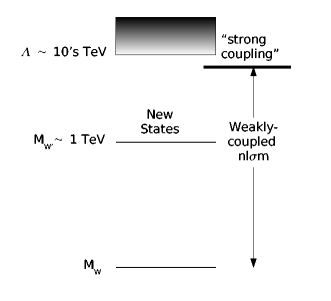
Figure 12: Fundamental scales of the three site model which are relevant to the calculation of the chiral-logarithmic corrections to the $S$ and $T$ parameters.

Finally, in the limit $M_{W}^{2}\ll M_{W^{\prime}}^{2}$, the couplings of the $U(1)$ and the $SU(2)_{2}$ gauge groups reduce to the corresponding SM values (up to corrections of ${\cal{O}}(M_{W}^{2}/M_{W^{\prime}}^{2})$) Foadi et al. (2004); Sekhar Chivukula et al. (2006):

$$g^{\prime}\simeq\frac{e}{c_{w}}\,\,\,\,\,,\,\,\,\,\,g\simeq\frac{e}{s_{w}}\,,$$ (119)

where we have used the tree-level definitions for $c_{w}$ and $s_{w}$ given by Eqs. (114) and (115). The chiral-logarithmic corrections to the $S$ and $T$ parameters for the three site model with delocalized fermions in the limit $M_{W}\ll M_{W^{\prime}}^{2}$ have been previously calculated in Feynman gauge ($\xi=1$) Matsuzaki et al. (2006) and Landau gauge ($\xi=0$) Chivukula et al. (2007) with identical results. In the present work, we use the exact expressions for the gauge couplings and mixing angles as given in Appendix B. By using the exact expressions for these parameters, our one-loop results retain sub-leading terms in $M_{W}^{2}/M_{W^{\prime}}^{2}$ which can be important for smaller values of $M_{W^{\prime}}$ (and $M_{Z^{\prime}}$). We have checked that our (unitary gauge) results in the limit $M_{W}^{2}\ll M_{W^{\prime}}^{2}$ agree with those of Refs. Matsuzaki et al. (2006) and Chivukula et al. (2007), thus proving the gauge-independence of our calculation.

VII.1 The $S$ Parameter

In the three site model with localized fermions, the $S$ parameter receives large corrections at tree level Foadi et al. (2004); Perelstein (2004). As alluded to earlier, however, this problem can be alleviated by allowing the light fermions to have a small coupling to the middle $SU(2)$ of Fig. 2. In this situation, the tree-level contribution to the $S$ parameter is given by Chivukula et al. (2005a); Anichini et al. (1995):

$$\alpha S_{tree}=\frac{4s_{w}^{2}M_{W}^{2}}{M_{W^{\prime}}^{2}}\biggl{(}1-\frac{x_{1}\,M_{W^{\prime}}^{2}}{2\,M_{W}^{2}}\biggr{)}+{\cal{O}}\biggl{(}\frac{M_{W}^{4}}{M_{W^{\prime}}^{4}}\biggr{)}\,.$$ (120)

For localized fermions $(x_{1}=0)$, where the fermions only directly couple to the end gauge groups of the moose diagram, $S_{tree}$ can only be made to agree with constraints from experimental data for very large values of $M_{W^{\prime}}$ ($\sim 2-3$ TeV). This spoils the restoration of unitarity in $V_{L}V_{L}$ scattering (where $V=W,Z$) which requires $M_{W^{\prime},Z^{\prime}}\leq 1.5$ TeV. However, from Eq. (120), we see that delocalizing the fermions provides a negative contribution to $S_{tree}$ which reduces the overall value at tree level. In fact, for $x_{1}=2M_{W}^{2}/M_{W^{\prime}}^{2}$, the tree-level contribution to $S$ completely vanishes, a situation which is referred to as ideal delocalization Sekhar Chivukula et al. (2005b). Thus, assessing the one-loop contributions to the $S$ parameter in the three site model becomes an important issue. In particular, the one-loop results are useful to answer an important question in Higgsless models: is there a unique choice for $x_{1}$ which is ideal for all orders or, in the case that the one-loop corrections are large, does $x_{1}$ need to be tuned order-by-order in perturbation theory in order to keep the value of $S$ within experimental limits. We will address this issue in the following.

Using the generic results for the PT self-energies from the previous sections and identifying poles in $\epsilon$ with the appropriate chiral logarithms as discussed above, the one-loop-corrected $S$ parameter in the three site model can be written as:

$$S_{3-site} = S_{tree}+A_{W}^{S}\,\log\biggl{(}\frac{\Lambda^{2}}{M_{W}^{2}}\biggr{)}+A_{W^{\prime}}^{S}\,\log\biggl{(}\frac{\Lambda^{2}}{M_{W^{\prime}}^{2}}\biggr{)}+S_{0}$$ (121)

$$= S_{tree}+A_{W}^{S}\,\log\biggl{(}\frac{M_{W^{\prime}}^{2}}{M_{W}^{2}}\biggr{)}+(A_{W^{\prime}}^{S}+A_{W}^{S})\,\log\biggl{(}\frac{\Lambda^{2}}{M_{W^{\prime}}^{2}}\biggr{)}+S_{0}$$

where, in the second line, the second term represents the contributions from the low-energy region (below $M_{W^{\prime}}$), the third term comprises the high-energy contributions and $S_{0}$ represents contributions from higher-dimension operators. Specifically, $S_{0}$ arises from the first two operators of Eq. (16). Inserting the expressions for the gauge fields in terms of the mass eigenstates (Eqs.(20)- (22)) into these operators, we can isolate shifts to the kinetic energy terms of the mass eigenstates. The effective Lagrangian describing these shifts takes the form Csaki et al. (2005):

$${\cal{L}}_{S_{0}}=-\frac{A}{4}\,F_{\mu\nu}F^{\mu\nu}-\frac{C}{4}\,Z_{\mu\nu}Z^{\mu\nu}+\frac{G}{2}\,F_{\mu\nu}Z^{\mu\nu}\,,$$ (122)

where $F_{\mu\nu}$ and $Z_{\mu\nu}$ are the usual Abelian field strengths and the coefficients $A,C$ and $G$ in the three site model are found to be:

$$A = -2(\alpha_{(1)1}\,b_{10}\,b_{20}+\alpha_{(2)1}\,b_{00}\,b_{10})\,,$$ (123)

$$C = -2(\alpha_{(1)1}\,b_{12}\,b_{22}+\alpha_{(2)1}\,b_{02}\,b_{12})\,,$$ (124)

$$G = \alpha_{(1)1}\,(b_{10}\,b_{22}+b_{12}\,b_{20})+\alpha_{(2)1}\,(b_{00}\,b_{12}+b_{02}\,b_{10})\,.$$ (125)

Finally, in terms of these coefficients, the contribution to $S$ from higher-dimension operators is Csaki et al. (2005):

$$S_{0}=\frac{4s_{w}^{2}c_{w}^{2}}{\alpha}\biggl{[}A-C-\frac{c_{w}^{2}-s_{w}^{2}}{s_{w}c_{w}}\,G\biggr{]}\,.$$ (126)

Thus, as stated earlier, the coefficients $\alpha_{(i)1}$ serve as counterterms which absorb the logarithmic divergences of Eq. (121), namely the $\log(\Lambda^{2}/M_{W^{\prime}}^{2})$ terms. In other words, these coefficients parameterize the effects of unknown physics above the scale $\Lambda$. Since we are mainly interested in studying the behavior of the one-loop results, we will set $S_{0}$ to zero in the following analysis.

At this point, an important check on our calculation is the numerical value of the coefficient ($A_{W}^{S}$) of the low-energy contribution. At energies well below $M_{W^{\prime}}$, the symmetries of the three site model are the same as those of the SM with a heavy Higgs boson Longhitano (1980, 1981). This implies that the dimension-two interactions in the two models at low energy are identical which, in turn, requires that the chiral-logarithmic corrections calculated from these interactions take the same form in the two theories Bando et al. (1985a, b, 1988a, 1988b). One would therefore expect that, in the limit that $M_{W}^{2}\ll M_{W^{\prime}}^{2}$, the coefficient of the low-energy contribution in the three site model should reduce to the value one would obtain in the SM with a heavy Higgs boson, i.e. Peskin and Takeuchi (1992); Herrero and Ruiz Morales (1994, 1995); Dittmaier and Grosse-Knetter (1996); Matias (1996); Alam et al. (1998):

$$A_{SM}^{S}=\frac{1}{12\pi}\,.$$ (127)

In the top panel of Fig. 13, we plot $A_{W}^{S}$ as a function of $M_{W^{\prime}}$ assuming ideal delocalization of the light fermions and that the mass of the $Z^{\prime}$ satisfies the relation $M_{Z^{\prime}}^{2}=M_{W^{\prime}}^{2}+(M_{Z}^{2}-M_{W}^{2})$. Clearly, $A_{W}^{S}$ saturates at the SM value for masses $M_{W^{\prime}}\simeq$ 1.5 TeV such that we find it useful to rewrite $A_{W}^{S}$ as:

$$A_{W}^{S}=\frac{1}{12\pi}+\kappa_{S}\,,$$ (128)

where $\kappa_{S}$ represents the contributions which decouple in the $M_{W^{\prime}}\to\infty$ limit . It is interesting to note, however, that the sub-leading terms in $M_{W}^{2}/M_{W^{\prime}}^{2}$ can have a significant impact for masses in the 300-700 GeV range leading to differences of a factor of two or so.

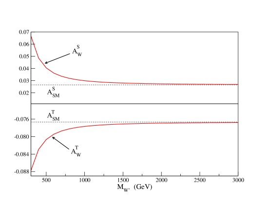
Figure 13: Top (Bottom) Panel: Coefficient for the low-energy contribution to $S_{3-site}$ ($T_{3-site}$) as a function of the $W^{\prime}$ mass. These plots assume ideal delocalization of the fermions and $M_{Z^{\prime}}^{2}=M_{W^{\prime}}^{2}+(M_{Z}^{2}-M_{W}^{2})$.

Precision electroweak data can now be used to constrain $S_{3-site}$ and, consequently, some of the relevant parameters (e.g., $M_{W^{\prime}}$, $\Lambda$ or the $\alpha_{(i)1}$ coefficients). However, this process is complicated by the fact that most global analyses are performed in the context of the SM with a fundamental Higgs boson. The physically-allowed region for $S$ (and $T$) is extracted in these analyses by performing a $\chi^{2}$ fit to fourteen precisely measured electroweak observables. For the case of a heavy Higgs boson, however, these analyses can be easily converted to a Higgsless scenario Bagger et al. (2000); Chivukula et al. (2000). This is accomplished by first subtracting the leading chiral-logarithmic contribution from a heavy Higgs boson Peskin and Takeuchi (1992); Herrero and Ruiz Morales (1994, 1995); Dittmaier and Grosse-Knetter (1996); Matias (1996); Alam et al. (1998); Chivukula and Evans (1999):

$$S_{Higgs}=\frac{1}{12\pi}\log\biggl{(}\frac{M_{H}^{2}}{M_{W}^{2}}\biggr{)}\,,$$ (129)

and then adding back in the contribution from Eq. (121). Thus, the value of the $S$ parameter to be used in the $\chi^{2}$ fit is simply given by:

$$S(S_{0},M_{W^{\prime}},\Lambda) = S_{ref}(M_{H}^{ref})-S_{Higgs}+S_{3-site}$$ (130)

$$\equiv [S_{ref}(M_{H}^{ref})-S_{Higgs}]+S_{1-loop}+S_{0}\,,$$

where $S_{ref}(M_{H}^{ref})$ is the SM $S$ parameter as a function of the reference Higgs boson mass, $M_{H}^{ref}$. In principle, for a heavy Higgs boson, $S_{ref}$ is dominated by the chiral-logarithmic term (Eq.(129)) such that any dependence on $M_{H}^{ref}$ cancels in the square-bracketed term in Eq.(130). The total one-loop contribution $S_{1-loop}$ from the three site model is then given by:

$$S_{1-loop}=S_{tree}+\delta S\,$$ (131)

where $\delta S$, the contribution from the loop diagrams alone, is:

$$\delta S=\frac{1}{12\pi}\,\log\biggl{(}\frac{M_{W^{\prime}}^{2}}{M_{W}^{2}}\biggr{)}+\kappa_{S}\,\log\biggl{(}\frac{M_{W^{\prime}}^{2}}{M_{W}^{2}}\biggr{)}+(A_{W^{\prime}}^{S}+A_{W}^{S})\,\log\biggl{(}\frac{\Lambda^{2}}{M_{W^{\prime}}^{2}}\biggr{)}\,.$$ (132)

Comparing Eq. (129) with the first term of Eq. (132) makes it clear that, in some sense, the role of the Higgs boson in the three site model is played by the $W^{\prime}$ Sekhar Chivukula et al. (2006). In other words, the Higgs mass, which cuts off the logarithmic divergences in the SM, is replaced by the mass of the $W^{\prime}$. In the following, this observation will allow us to compare our one-loop results directly with experimental constraints to obtain bounds on the three site model without carrying out the full analysis outlined above. This is accomplished provided we identify the mass of the $W^{\prime}$ with the corresponding Higgs boson mass used in the global analysis. In particular, we will consider two values: $M_{W^{\prime}}=M_{H}^{ref}=340$ GeV and 1 TeV, for which the 90% C.L. limits on $S$ are Yao et al. (2006):

$$-0.33\leq S\leq 0.05\,\,\,\,\,\,\,\,(M_{W^{\prime}}=M_{H}^{ref}=340\,\,\mbox{GeV})$$ (133)

$$-0.45\leq S\leq 0.00\,\,\,\,\,\,\,\,(M_{W^{\prime}}=M_{H}^{ref}=1\,\,\mbox{TeV})\,.$$ (134)

At this point, the one-loop result $\delta S$ is a function of four parameters: the masses $M_{W^{\prime}},M_{Z^{\prime}}$, the delocalization parameter $x_{1}$ and the cutoff scale $\Lambda$. In comparing the three site model to experimental limits, we will identify the mass of the $W^{\prime}$ with the particular Higgs boson mass used in the global fit. Thus, we are left with only $M_{Z^{\prime}}$, $x_{1}$ and $\Lambda$ as free parameters. In Fig. 14, we plot $S_{1-loop}$ as a function of the mass splitting $M_{Z^{\prime}}-M_{W^{\prime}}$ for $M_{W^{\prime}}$ = 340 GeV (top panel) and $M_{W^{\prime}}$ = 1 TeV (bottom panel). We also consider two values of the cutoff $\Lambda$ for each mass. In these plots, we have assumed ideal delocalization for the light fermions such that $S_{tree}=0$. For both $W^{\prime}$ masses considered, we note that the corrections to $S$ in the three site model can be large ($\sim{\cal{O}}(\pm 1)$) even with $S_{tree}=0$. Indeed, there appear to be only small windows in the mass difference where $S_{1-loop}$ can be brought into approximate agreement with the experimental constraints. In particular, for $M_{W^{\prime}}=340$ GeV, the allowed regions are $M_{Z^{\prime}}-M_{W^{\prime}}\approx 0.2$ GeV where the $Z^{\prime}$ and $W^{\prime}$ are nearly degenerate and $M_{Z^{\prime}}-M_{W^{\prime}}\approx M_{Z}-M_{W}$. Finally, it is interesting to note that in both cases, $S_{1-loop}$ becomes nearly independent of $\Lambda$ above $M_{Z^{\prime}}-M_{W^{\prime}}\approx M_{Z}-M_{W}$ which (from Eq. (132)) implies:

$$A_{W}^{S}+A_{W^{\prime}}^{S}\simeq 0\,,$$ (135)

in this range.

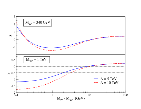
Figure 14: The $S$ parameter in the three site Higgsless model at the one-loop level as a function of the mass difference $M_{Z^{\prime}}-M_{W^{\prime}}$ for different values of the cutoff of the effective theory, $\Lambda$. Ideal delocalization is assumed in these plots such that $S_{tree}$ = 0 (120). The upper (lower) panel corresponds to $M_{W^{\prime}}$ = 340 GeV (1 TeV). The horizontal dashed lines indicate the 90% C.L. bounds on the $S$ parameter for Higgs boson of the same mass Yao et al. (2006).

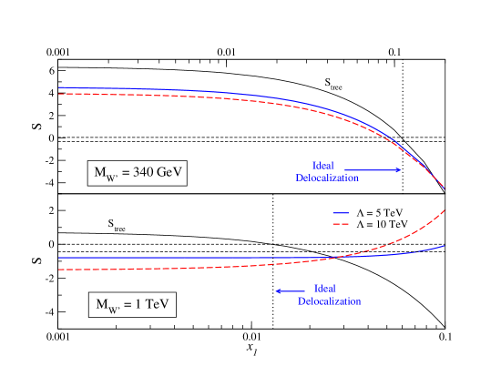
Figure 15: The $S$ parameter in the three site Higgsless model at the one-loop level as a function of the delocalization parameter $x_{1}$ for $M_{W^{\prime}}$ = 340 GeV (top) and 1 TeV (bottom). The 90% C.L. limits on $S$ for a Higgs boson of the same mass are indicated by horizontal dashed lines Yao et al. (2006).

Finally, we consider the dependence of $S_{1-loop}$ (and $S_{tree}$) on the delocalization parameter $x_{1}$ as shown in Fig. 15. Again, we consider two values of $M_{W^{\prime}}$ and we have set $M_{Z^{\prime}}^{2}=M_{W^{\prime}}^{2}+(M_{Z}^{2}-M_{W}^{2})$. We denote by a vertical dotted line the point at which $S_{tree}$ = 0. The dependence of the $S$ parameter on the delocalization procedure itself is an important issue in the three site model and other Higgsless models in general. The outstanding question is whether $x_{1}$ must be tuned order-by-order in perturbation theory in such a way to bring $S$ into agreement with precision electroweak data or the value of $x_{1}$ which cancels $S_{tree}$ is ideal at all orders. As we see from the top panel of Fig. 15, going from tree level to one-loop level requires a tuning of $x_{1}$ at the $\sim$ 20-30% level for smaller values of $M_{W^{\prime}}$. This relatively small tuning is due to the fact that the total contribution to $S$ is dominated by the tree-level value. However, as evidenced by the bottom panel, the tuning becomes much more severe for heavier masses. Indeed, for $M_{W^{\prime}}=$ 1 TeV, one must tune $x_{1}$ by a factor of $\sim$ 5 in order to reconcile $S_{1-loop}$ with the constraints from data. Of course, this conclusion is highly dependent on the particular choice of $M_{Z^{\prime}}$ (see Fig. 14), but the relationship between $M_{Z^{\prime}}$ and $M_{W^{\prime}}$ we have chosen for these plots is a preferred one in the three site model since it results in maximal suppression of unitarity-violating terms in $W_{L}W_{L}$ scattering (see Fig. 2 of Ref. Foadi et al. (2004)).

VII.2 The $T$ Parameter

At tree level in the three site model, the $T$ parameter exactly vanishes due to the presence of an $SU(2)$ custodial symmetry. When the fermions are delocalized to negate large corrections to the $S$ parameter, the SM fermions develop heavy partners with the same SM quantum numbers. At the one-loop level, these new fermions, especially the partners of the top and bottom quarks, can make potentially sizable contributions to the $T$ parameter Sekhar Chivukula et al. (2006). We will not consider these corrections here, but we note that they are typically of the same size and opposite sign relative to the gauge sector contributions which we discuss below. The end result is a large cancelation between the two contributions such that the $T$ parameter is safe in the three site model even at the one-loop level.

The one-loop, chiral-logarithmic corrections to $T$ from the gauge sector of the three site model naturally separate into low- and high-energy contributions:

$$T_{3-site} = A_{W}^{T}\,\log\biggl{(}\frac{\Lambda^{2}}{M_{W}^{2}}\biggr{)}+A_{W^{\prime}}^{T}\,\log\biggl{(}\frac{\Lambda^{2}}{M_{W^{\prime}}^{2}}\biggr{)}+T_{0}$$ (136)

$$= A_{W}^{T}\,\log\biggl{(}\frac{M_{W^{\prime}}^{2}}{M_{W}^{2}}\biggr{)}+(A_{W^{\prime}}^{T}+A_{W}^{T})\,\log\biggl{(}\frac{\Lambda^{2}}{M_{W^{\prime}}^{2}}\biggr{)}+T_{0}\,,$$

where $T_{0}$ represents the contribution from the dimension-two operator of Eq. (14). The expression for $T_{0}$ can be extracted by inserting the expansions of the gauge fields in terms of the mass eigenstates (Eqs. (20) and (21)) into Eq. (14). Isolating corrections to the SM-like $Z$ boson mass, we find that ${\cal{L}}_{2}^{\prime}$ produces a term of the form:

$${\cal{L}}_{T^{0}}=-\frac{z}{2}\,M_{Z}^{2}\,Z_{\mu}Z^{\mu}\,,$$ (137)

where $z$ is given by:

$$z=\frac{\beta_{(2)}\,f_{1}^{2}}{2M_{Z}^{2}}\,(g^{\prime}\,b_{02}-\tilde{g}\,b_{12})^{2}\,.$$ (138)

In contrast, higher-dimension operators do not contribute to a shift in the $W$ boson mass and $T_{0}$ is given by Csaki et al. (2005):

$$T_{0}=-z=-\frac{\beta_{(2)}\,f_{1}^{2}}{2M_{Z}^{2}}\,(g^{\prime}\,b_{02}-\tilde{g}\,b_{12})^{2}\,.$$ (139)

Combining Eq. (139) with Eq. (136) makes it clear that the $\beta_{(2)}$ coefficient acts as a counterterm for the $T$ parameter. Therefore, as in the previous section, we will set $T_{0}$ to zero for our analysis.

As a check of our calculation for $T$ in the three site model, we plot the coefficient of the low-energy contribution, $A_{W}^{T}$, in the bottom panel of Fig. (13). In the energy region below $M_{W^{\prime}}$, the operators which generate corrections to $T$ in the three site model are identical to the operators of the SM with a heavy Higgs boson Bando et al. (1985a, b, 1988a, 1988b). Therefore, in the limit $M_{W}^{2}\ll M_{W^{\prime}}^{2}$, $A_{W}^{T}$ reduces to the SM value: Peskin and Takeuchi (1992); Herrero and Ruiz Morales (1994, 1995); Dittmaier and Grosse-Knetter (1996); Matias (1996); Alam et al. (1998):

$$A_{SM}^{T}=-\frac{3}{16\pi c_{w}^{2}}\,,$$ (140)

as seen in the bottom panel of Fig. (13). Thus, to simplify our analysis, we find it convenient to rewrite the low-energy coefficient as:

$$A_{W}^{T}=-\frac{3}{16\pi c_{w}^{2}}+\kappa_{T}\,,$$ (141)

where $\kappa_{T}$ parameterizes the piece of the low-energy contributions which decouples in the large $M_{W^{\prime}}$ limit. In contrast to the low-energy coefficient for the $S$ parameter, we see that the sub-leading terms in $M_{W}^{2}/M_{W^{\prime}}^{2}$ have a much smaller effect on $A_{W}^{T}$ for lower values of $M_{W^{\prime}}$.

In analogy to the previous section, the one-loop prediction for $T$ can now be compared to precision electroweak data in order to constrain some (or all) of the parameters of the three site model. The analysis follows along the same lines as the case of the $S$ parameter. First, the chiral-logarithmic contribution from a heavy Higgs boson Peskin and Takeuchi (1992); Herrero and Ruiz Morales (1994, 1995); Dittmaier and Grosse-Knetter (1996); Matias (1996); Alam et al. (1998); Chivukula and Evans (1999):

$$T_{Higgs}=-\frac{3}{16\pi c_{w}^{2}}\log\biggl{(}\frac{M_{H}^{2}}{M_{W}^{2}}\biggr{)}\,,$$ (142)

must be subtracted from the global analysis. Then, adding back in the contribution from Eq. (136), the value of $T$ to be used in the $\chi^{2}$ fit is given by:

$$T(T_{0},M_{W^{\prime}},\Lambda) = T_{ref}(M_{H}^{ref})-T_{Higgs}+T_{3-site}$$ (143)

$$\equiv [T_{ref}(M_{H}^{ref})-T_{Higgs}]+T_{1-loop}+T_{0}\,,$$ (144)

where $T_{ref}(M_{H}^{ref})$ is the SM $T$ parameter as a function of the reference Higgs boson mass, $M_{H}^{ref}$. For large enough values of the Higgs boson mass, $T_{ref}$ is dominated by the chiral-logarithmic contribution from the Higgs such that the quantity in square brackets is independent of $M_{H}^{ref}$. Lastly, the one-loop contribution $T_{1-loop}$ is found to be:

$$T_{1-loop}=-\frac{3}{16\pi c_{w}^{2}}\,\log\biggl{(}\frac{M_{W^{\prime}}^{2}}{M_{W}^{2}}\biggr{)}+\kappa_{T}\,\log\biggl{(}\frac{M_{W^{\prime}}^{2}}{M_{W}^{2}}\biggr{)}+(A_{W^{\prime}}^{T}+A_{W}^{T})\,\log\biggl{(}\frac{\Lambda^{2}}{M_{W^{\prime}}^{2}}\biggr{)}\,.$$ (145)

Again, comparing Eq. (142) with the first term of Eq. (145), we see that the cutoff of the logarithmic divergences from the low-energy sector, which is typically provided by the Higgs boson mass, is being played by the $W^{\prime}$ mass. Lastly, we mention that, given the potentially large (and positive definite) corrections coming from the fermionic sector, we will not exhibit any limits in the following plots. To be consistent, though, we will consider the same mass values as in the previous section: $M_{W^{\prime}}=M_{H}^{ref}=340$ GeV and 1 TeV, for which the 90% C.L. limits on $T$ are Yao et al. (2006):

$$-0.15\leq T\leq 0.27\,\,\,\,\,\,\,\,(M_{W^{\prime}}=M_{H}^{ref}=340\,\,\mbox{GeV})$$ (146)

$$0.02\leq T\leq 0.42\,\,\,\,\,\,\,\,(M_{W^{\prime}}=M_{H}^{ref}=1\,\,\mbox{TeV})\,.$$ (147)

First, we consider the dependence of $T$ on the mass difference $M_{Z^{\prime}}-M_{W^{\prime}}$ in Fig. 16. In comparison to the results for the $S$ parameter, we note that the overall size of the corrections to $T$ are much smaller. We also point out that, for $M_{Z^{\prime}}-M_{W^{\prime}}\geq 1$ GeV, the corrections are of the same size and opposite sign relative to the fermionic contribution Sekhar Chivukula et al. (2006). The result is a large cancelation which brings the full three site model contribution to $T$ within the experimental bounds given above. Finally, we again note that, above $M_{Z^{\prime}}-M_{W^{\prime}}=M_{Z}-M_{W}$, the one-loop results become nearly independent of the cutoff scale $\Lambda$, which implies:

$$A_{W}^{T}+A_{W^{\prime}}^{T}\simeq 0$$ (148)

in this range.

Finally, we consider the $x_{1}$ dependence of the one-loop contributions to $T$. Since $x_{1}$ respects the custodial symmetry present in the three site model, one would expect this dependence to be negligible Sekhar Chivukula et al. (2006). In Fig. 17, we plot our results as a function of $x_{1}$ for two separate $M_{W^{\prime}}$ values. From these plots, it is apparent that the one-loop corrections are, in fact, independent of $x_{1}$ over the majority of the range considered. Only at the larger values of $x_{1}$ do the values of $T$ start to show some dependence. However, these larger values of $x_{1}$ are typically ruled out by experimental constraints on the $ZWW$ vertex Sekhar Chivukula et al. (2006).

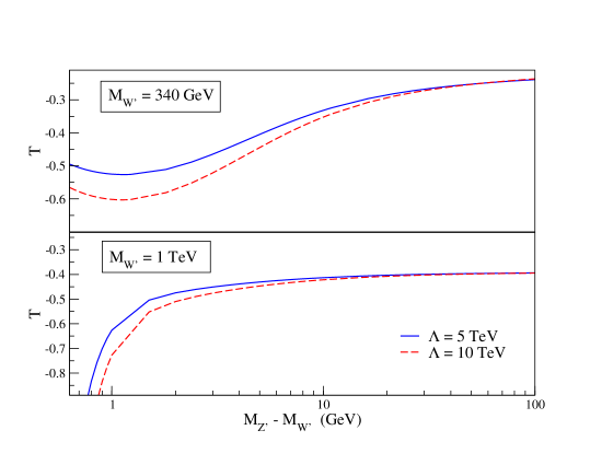
Figure 16: One-loop, chiral-logarithmic corrections to the $T$ parameter in the three site model as a function of the mass difference $M_{Z^{\prime}}-M_{W^{\prime}}$ and $\Lambda$. The lower (upper) panel corresponds to $M_{W^{\prime}}$ = 340 GeV (1 TeV) and we have assumed ideally delocalized fermions.

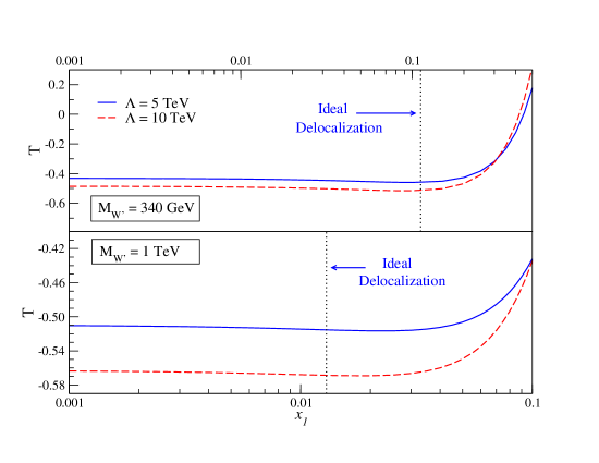
Figure 17: One-loop, chiral-logarithmic corrections to the $T$ parameter in the three site model as a function of the delocalization parameter $x_{1}$. The lower (upper) panel corresponds to $M_{W^{\prime}}$ = 340 GeV (1 TeV). The point of ideal fermion delocalization is depicted by a vertical dotted line.

VIII Conclusions

We have calculated the one-loop corrections to the $S$ and $T$ parameters in models which contain extra vector gauge bosons, but which are devoid of any fundamental scalars (i.e., Higgs bosons). We have performed this calculation using a novel application of the Pinch Technique (PT) which requires including certain pieces from vertex and box corrections, along with the usual loop-corrected two-point functions, in order to obtain gauge-independent expressions for the gauge boson self-energies Degrassi and Sirlin (1992b, a); Papavassiliou and Sirlin (1994); Degrassi et al. (1993). All of the diagrams needed to construct the PT self-energies have been calculated using generic couplings for the gauge boson self-interactions as well as the interactions between the light fermions and gauge bosons. This permits our results to be applied to various models by simply identifying the generic couplings of our expressions with the fundamental parameters of a specific model. To conclude our algorithm, we have demonstrated how to assemble all of the one-loop diagrams in order to obtain gauge-independent expressions for the $S$ and $T$ parameters.

As an example of how the algorithm presented here may be applied, we have calculated the one-loop, chiral-logarithmic corrections to $S$ and $T$ in the highly-deconstructed three site model Foadi et al. (2004); Perelstein (2004); Sekhar Chivukula et al. (2006). The gauge sector of this model, which is identical to that of the BESS model Casalbuoni et al. (1985, 1987), consists of a SM-like set of gauge bosons (massless photon and light vector gauge bosons, $W^{\pm}$ and $Z$) plus an extra set of heavy vector gauge bosons ($W^{\prime\pm}$ and $Z^{\prime}$). At tree level, mixing between the various gauge eigenstates generates a large contribution to the $S$ parameter. However, when the fermions of the model are allowed to derive their couplings from all three gauge groups, they provide a negative contribution to the $S$ parameter which can reduce or even negate the large contribution from the gauge sector. This underlines the need for a one-loop calculation of the $S$ parameter in this model and other Higgsless models where similar delocalization procedures can be employed to reduce large corrections from the extended gauge sectors. The $T$ parameter in the three site model vanishes at tree level due to the presence of a custodial $SU(2)$ symmetry. Thus, assessing the one-loop corrections to $T$ in this model also becomes important.

The loop-corrected values of the $S$ and $T$ parameters in the three site model were previously calculated in both the Feynman Matsuzaki et al. (2006) and Landau Chivukula et al. (2007) gauges in the limit $M_{W}^{2}\ll M_{W^{\prime}}^{2}$. In the calculation presented here, however, we have worked with the exact expressions for the free parameters of the model. In other words, we have retained sub-leading terms in $M_{W}^{2}/M_{W^{\prime}}^{2}$ which can be important for smaller values of $M_{W^{\prime}}$. We have compared our results, which were obtained by employing the unitary gauge, in the limit $M_{W}^{2}\ll M_{W^{\prime}}^{2}$ with those of Refs. Matsuzaki et al. (2006) and Chivukula et al. (2007) and found excellent agreement. This was an important check of our algorithm and, in fact, proves the gauge-independence of our results.

In our approach, the one-loop expressions for $S$ and $T$ in the three site model reduce to functions of only four parameters: the cutoff of the effective theory ($\Lambda$), the degree of delocalization for the light fermions ($x_{1}$) and the masses of the heavy gauge bosons ($M_{W^{\prime}}$ and $M_{Z^{\prime}}$). The first of these only appears in the chiral logarithms which are present due to the non-renormalizability of the theory and is assumed to be in the range 5 TeV $<\Lambda<$ 10 TeV. We have shown that, for both $S$ and $T$, the low-energy contribution in the three site model reduces to the usual SM value with the Higgs boson mass dependence replaced by the $W^{\prime}$ mass.

In particular, we studied the dependence of the $S$ and $T$ parameters on the mass difference $M_{Z^{\prime}}-M_{W^{\prime}}$ and the delocalization parameter $x_{1}$. While the dependence of $T$ on these quantities is minimal, the $S$ parameter exhibits strong dependence on both and, in fact, can only be reconciled with experimental limits in small ranges of both quantities. The dependence of $S$ on $x_{1}$ is of particular interest in the three site model. The outstanding issue is whether or not $x_{1}$ must be tuned order-by-order in perturbation theory to bring $S$ into agreement with experimental constraints. In our analysis, we have found that the tuning is minimal for lighter $W^{\prime}$ masses. This is mainly due to dominance of the tree-level contribution over the one-loop contributions for small $M_{W^{\prime}}$. However, for larger masses, the tuning can be much more severe. In particular, for $M_{W^{\prime}}$ = 1 TeV, we found that $x_{1}$ must be tuned by a factor of five in going from tree level to the one-loop level.

Finally, it should be stated that our calculation is not exclusive to Higgsless models. As mentioned in the Introduction, one-loop corrections to the VGB self-energies can always be separated into gauge-invariant contributions from fermions, scalars and gauge bosons. In other words, our calculation could be used to calculate the gauge-bosonic contributions to oblique parameters in models which contain fundamental (or composite) Higgs bosons.

Appendix A Scalar Integrals and Tensor Coefficients

The scalar integrals that appear in the calculation of the PT self-energies are the one-point integral $A_{0}(M)$:

$$A_{0}(M)\equiv\int\frac{d^{n}k}{(2\pi)^{n}}\frac{1}{k^{2}-M^{2}}\,,$$ (149)

and the two-point integral $B_{0}(q^{2};M_{1},M_{2})$:

$$B_{0}(q^{2};M_{1},M_{2})=\int\frac{d^{n}k}{(2\pi)^{n}}\frac{1}{(k^{2}-M_{1}^{2})((k+q)^{2}-M_{2}^{2})}\,.$$ (150)

In order to extract the chiral-logarithmic corrections, we only need to calculate the poles of the scalar integrals which are then identified with the appropriate chiral logarithms:

$$A_{0}(M)\bigl{|}_{pole} = \frac{i}{16\pi^{2}\epsilon}M^{2}\to\frac{i}{16\pi^{2}}\,\log\biggl{(}\frac{\Lambda^{2}}{M^{2}}\biggr{)}M^{2}\,,$$ (151)

and:

$$B_{0}(q^{2};M_{1},M_{2})\bigl{|}_{pole} = \frac{i}{16\pi^{2}\epsilon}\to\frac{i}{16\pi^{2}}\,\log\biggl{(}\frac{\Lambda^{2}}{M^{2}}\biggr{)}\,.$$ (152)

The tensor integrals that arise in our calculation consist of the rank-one and rank-two two-point integrals:

$$B^{\mu}(q^{2};M_{1},M_{2}) = \int\frac{d^{n}k}{(2\pi)^{n}}\frac{k^{\mu}}{(k^{2}-M_{1}^{2})((k+q)^{2}-M_{2}^{2})}\,,$$ (153)

$$B^{\mu\nu}(q^{2};M_{1},M_{2}) = \int\frac{d^{n}k}{(2\pi)^{n}}\frac{k^{\mu}k^{\nu}}{(k^{2}-M_{1}^{2})((k+q)^{2}-M_{2}^{2})}\,.$$ (154)

Tensor integrals can always be expanded in terms of external momenta and the metric tensor $g^{\mu\nu}$ Passarino and Veltman (1979). Specifically, the integrals in Eqs. (153) and (154) can be written as

$$B^{\mu}(q^{2};M_{1},M_{2}) = q^{\mu}\,B_{11}(q^{2};M_{1},M_{2})$$ (155)

$$B^{\mu\nu}(q^{2};M_{1},M_{2}) = q^{\mu}q^{\nu}\,B_{21}(q^{2};M_{1},M_{2})+g^{\mu\nu}\,B_{22}(q^{2};M_{1},M_{2})\,.$$ (156)

Finally, equating the the tensor integral with its respective expansion and contracting both sides with external momenta and $g^{\mu\nu}$, one can solve the system of equations for the coefficients in Eqs. (155) and (156) in terms of the scalar integrals. Specifically,:

$$B_{11}(q^{2};M_{1},M_{2}) = \frac{1}{2q^{2}}\biggl{[}A_{0}(M_{1})-A_{0}(M_{2})-(q^{2}+M_{1}^{2}-M_{2}^{2})B_{0}(q^{2};M_{1},M_{2})\biggr{]}$$ (157)

$$B_{21}(q^{2};M_{1},M_{2}) = \frac{1}{3q^{2}}\biggl{[}A_{0}(M_{2})+2(M_{2}^{2}-M_{1}^{2}-q^{2})\,B_{11}(q^{2};M_{1},M_{2})$$ (158)

$$\,\,\,\,\,\,\,\,\,\,\,\,\,\,\,\,\,\,\,\,-M_{1}^{2}\,B_{0}(q^{2};M_{1},M_{2})\biggr{]}$$

$$B_{22}(q^{2};M_{1},M_{2}) = \frac{1}{3}\biggl{[}\frac{1}{2}A_{0}(M_{2})+M_{1}^{2}\,B_{0}(q^{2};M_{1},M_{2})$$ (159)

$$\,\,\,\,\,\,\,\,\,\,\,\,\,\,\,\,\,\,\,\,-\frac{1}{2}(M_{2}^{2}-M_{1}^{2}-q^{2})B_{11}(q^{2};M_{1},M_{2})\biggr{]}\,.$$

Appendix B Formulae for the Three Site Model

In this appendix, we summarize the relevant formulae for the three site model Foadi et al. (2004); Perelstein (2004); Sekhar Chivukula et al. (2006). We begin by finding the mass eigenvalues. First, in the charged sector, the mass matrix is:

$$M_{CC}=\frac{1}{4}\left(\begin{array}[]{cc}\tilde{g}^{2}(f_{1}^{2}+f_{2}^{2})&\,\,\,\,\,-g\tilde{g}f_{2}^{2}\\ -g\tilde{g}f_{2}^{2}&g^{2}f_{2}^{2}\end{array}\right)\,,$$ (160)

for which we find the eigenvalues:

$$M_{W,W^{\prime}}^{2}=\frac{1}{8}\biggl{\{}\tilde{g}^{2}(f_{1}^{2}+f_{2}^{2})+g^{2}\,f_{2}^{2}\mp\biggl{[}(\tilde{g}^{2}(f_{1}^{2}+f_{2}^{2})+g^{2}\,f_{2}^{2})^{2}-4f_{1}^{2}f_{2}^{2}g^{2}\tilde{g}^{2}\biggr{]}^{\frac{1}{2}}\biggr{\}}\,,$$ (161)

where the SM-like $W$ is identified with the lighter of the two eigenvalues.

Next, the mass matrix for the neutral sector is:

$$M_{NC}=\frac{1}{8}\left(\begin{array}[]{ccc}g^{\prime 2}f_{1}^{2}&-g^{\prime}\tilde{g}f_{1}^{2}&0\\ -g^{\prime}\tilde{g}f_{1}^{2}&\,\,\,\,\tilde{g}^{2}(f_{1}^{2}+f_{2}^{2})&\,\,\,\,-g\tilde{g}f_{2}^{2}\\ 0&-g\tilde{g}f_{2}^{2}&g^{2}f_{2}^{2}\end{array}\right)\,.$$ (162)

Diagonalizing this matrix results in a massless eigenstate, which is identified with the SM photon, and two massive states with mass eigenvalues:

$$M_{Z,Z^{\prime}} = \frac{1}{16}\biggl{\{}\tilde{g}^{2}(f_{1}^{2}+f_{2}^{2})+g^{\prime 2}f_{1}^{2}+g^{2}f_{2}^{2}$$ (163)

$$\,\,\,\,\,\,\,\,\mp\biggl{[}(\tilde{g}^{2}(f_{1}^{2}+f_{2}^{2})+g^{\prime 2}f_{1}^{2}+g^{2}f_{2}^{2})^{2}-4f_{1}^{2}f_{2}^{2}(g^{2}\tilde{g}^{2}+g^{\prime 2}(g^{2}+\tilde{g}^{2}))\biggr{]}^{\frac{1}{2}}\biggr{\}}\,.$$

where the SM-like $Z$ is identified with the lighter of the two states.

In its original form, the three site model contains five free parameters: $g,g^{\prime},\tilde{g},f_{1}$ and $f_{2}$. For our analysis, we find it convenient to exchange these parameters for the four masses ($M_{W},M_{Z},M_{W^{\prime}}$ and $M_{Z^{\prime}}$) defined through Eqs. (161) and (163). As the fifth parameter, we choose the electromagnetic coupling $e$ which is defined by Eq. (17). Solving these equations for the original parameters, we find Foadi et al. (2004):

$$g^{\prime 2} = {e^{2}M_{Z}^{2}M_{Z^{\prime}}^{2}\over M_{W}^{2}M_{W^{\prime}}^{2}}\ ,$$

$$\tilde{g}^{2} = g^{\prime 2}\left[{(M_{W}^{2}+M_{W^{\prime}}^{2})(M_{Z}^{2}+M_{Z^{\prime}}^{2}-M_{W}^{2}-M_{W^{\prime}}^{2})+M_{W}^{2}M_{W^{\prime}}^{2}-M_{Z}^{2}M_{Z^{\prime}}^{2}\over(M_{Z}^{2}+M_{Z^{\prime}}^{2}-M_{W}^{2}-M_{W^{\prime}}^{2})^{2}}\right]\ ,$$

$$g^{2} = {g^{\prime 2}M_{W}^{2}M_{W^{\prime}}^{2}}\left[{(M_{W}^{2}+M_{W^{\prime}}^{2})(M_{Z}^{2}+M_{Z^{\prime}}^{2}-M_{W}^{2}-M_{W^{\prime}}^{2})+M_{W}^{2}M_{W^{\prime}}^{2}-M_{Z}^{2}M_{Z^{\prime}}^{2}\over(M_{Z}^{2}-M_{W}^{2})(M_{Z^{\prime}}^{2}-M_{W^{\prime}}^{2})(M_{Z^{\prime}}^{2}-M_{W}^{2})(M_{W^{\prime}}^{2}-M_{Z}^{2})}\right]\ ,$$

$$f_{1}^{2} = {4\over g^{\prime 2}}(M_{Z}^{2}+M_{Z^{\prime}}^{2}-M_{W}^{2}-M_{W^{\prime}}^{2})\ ,$$

$$f_{2}^{2} = {16M_{W}^{2}M_{W^{\prime}}^{2}\over\tilde{g}^{2}g^{2}f_{1}^{2}}\ ,$$ (164)

where we have assumed in the above relations that $M_{Z^{\prime}}>M_{W^{\prime}}$.

Finally, in order to compute the couplings relevant to the calculation of the $S$ and $T$ parameters, we need to calculate the mixing angles defined through Eqs. (18)-(22). First, in the charged sector, we have $a_{11}=a_{22}$ and $a_{12}=-a_{21}$ where:

$$a_{11} = \left[{M_{W^{\prime}}^{2}(M_{W^{\prime}}^{2}-M_{Z}^{2})(M_{Z^{\prime}}^{2}-M_{W^{\prime}}^{2})\over M_{W^{\prime}}^{2}(M_{W^{\prime}}^{2}-M_{Z}^{2})(M_{Z^{\prime}}^{2}-M_{W^{\prime}}^{2})+M_{W}^{2}(M_{Z^{\prime}}^{2}-M_{W}^{2})(M_{Z}^{2}-M_{W}^{2})}\right]^{1/2}\ ,$$

$$a_{12} = \left[{M_{W}^{2}(M_{Z^{\prime}}^{2}-M_{W}^{2})(M_{Z}^{2}-M_{W}^{2})\over M_{W^{\prime}}^{2}(M_{W^{\prime}}^{2}-M_{Z}^{2})(M_{Z^{\prime}}^{2}-M_{W^{\prime}}^{2})+M_{W}^{2}(M_{Z^{\prime}}^{2}-M_{W}^{2})(M_{Z}^{2}-M_{W}^{2})}\right]^{1/2}\ .$$ (165)

The mixing angles in the neutral sector are given by:

$$b_{00} = \frac{e}{g^{\prime}}\,,$$ (166)

$$b_{10} = \frac{e}{\tilde{g}}\,,$$

$$b_{20} = \frac{e}{g}\,,$$

$$b_{01} = -\left[{(M_{Z^{\prime}}^{2}-M_{W}^{2})(M_{Z^{\prime}}^{2}-M_{W^{\prime}}^{2})\over M_{Z^{\prime}}^{2}(M_{Z^{\prime}}^{2}-M_{Z}^{2})}\right]^{1/2}\ ,$$

$$b_{11} = \left[{(M_{Z^{\prime}}^{2}-M_{W}^{2})(M_{Z^{\prime}}^{2}-M_{W^{\prime}}^{2})\over M_{Z^{\prime}}^{2}(M_{Z^{\prime}}^{2}-M_{Z}^{2})\Bigl{[}(M_{W}^{2}+M_{W^{\prime}}^{2})(M_{Z}^{2}+M_{Z^{\prime}}^{2}-M_{W}^{2}-M_{W^{\prime}}^{2})+M_{W}^{2}M_{W^{\prime}}^{2}-M_{Z}^{2}M_{Z^{\prime}}^{2}\Bigr{]}}\right]^{1/2}$$

$$\times\biggl{(}M_{W^{\prime}}^{2}+M_{W}^{2}-M_{Z}^{2}\biggr{)}\ ,$$

$$b_{21} = -\left[{M_{W}^{2}M_{W^{\prime}}^{2}(M_{Z}^{2}-M_{W}^{2})(M_{W^{\prime}}^{2}-M_{Z}^{2})\over M_{Z^{\prime}}^{2}(M_{Z^{\prime}}^{2}-M_{Z}^{2})\Bigl{[}(M_{W}^{2}+M_{W^{\prime}}^{2})(M_{Z}^{2}+M_{Z^{\prime}}^{2}-M_{W}^{2}-M_{W^{\prime}}^{2})+M_{W}^{2}M_{W^{\prime}}^{2}-M_{Z}^{2}M_{Z^{\prime}}^{2}\Bigr{]}}\right]^{1/2}\ ,$$

$$b_{02} = -\left[{(M_{Z}^{2}-M_{W}^{2})(M_{W^{\prime}}^{2}-M_{Z}^{2})\over M_{Z}^{2}(M_{Z^{\prime}}^{2}-M_{Z}^{2})}\right]^{1/2}\ ,$$

$$b_{12} = \left[{(M_{Z}^{2}-M_{W}^{2})(M_{W^{\prime}}^{2}-M_{Z}^{2})\over M_{Z}^{2}(M_{Z^{\prime}}^{2}-M_{Z}^{2})\Bigl{[}(M_{W}^{2}+M_{W^{\prime}}^{2})(M_{Z}^{2}+M_{Z^{\prime}}^{2}-M_{W}^{2}-M_{W^{\prime}}^{2})+M_{W}^{2}M_{W^{\prime}}^{2}-M_{Z}^{2}M_{Z^{\prime}}^{2}\Bigr{]}}\right]^{1/2}$$

$$\times\biggl{(}M_{W^{\prime}}^{2}+M_{W}^{2}-M_{Z^{\prime}}^{2}\biggr{)}\ ,$$

$$b_{22} = \left[{M_{W}^{2}M_{W^{\prime}}^{2}(M_{Z^{\prime}}^{2}-M_{W}^{2})(M_{Z^{\prime}}^{2}-M_{W^{\prime}}^{2})\over M_{Z}^{2}(M_{Z^{\prime}}^{2}-M_{Z}^{2})\Bigl{[}(M_{W}^{2}+M_{W^{\prime}}^{2})(M_{Z}^{2}+M_{Z^{\prime}}^{2}-M_{W}^{2}-M_{W^{\prime}}^{2})+M_{W}^{2}M_{W^{\prime}}^{2}-M_{Z}^{2}M_{Z^{\prime}}^{2}\Bigr{]}}\right]^{1/2}.$$

Appendix C Pinch Contributions from Light-Heavy Gauge Boson Mixing

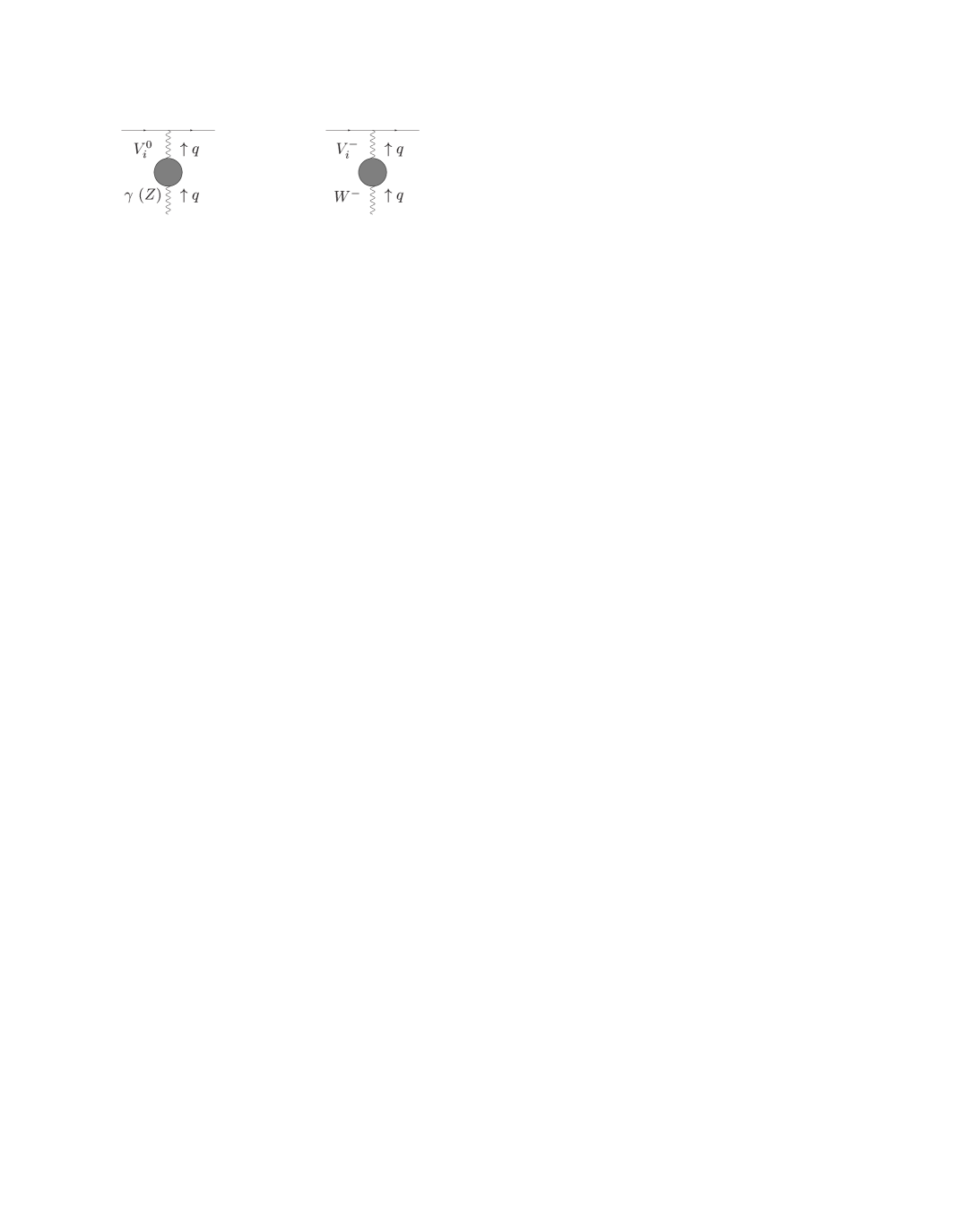
Figure 18: One-loop corrections which result in mixing between the light and heavy gauge bosons. In the limit where the mass of the heavy gauge boson is much larger than the momentum $q$, these diagrams give rise to pinch-like contributions.

In addition to the pinch contributions arising from vertex corrections as discussed in Sections IV.2 and V.2, one-loop diagrams which mix the light and heavy gauge boson propagators can also give rise to pinch-like contributions. The diagrams which contribute to these types of corrections are depicted in Fig. 18 for both the neutral- and charged-current cases. The amplitudes for these corrections can easily be calculated by using the results of Sections  IV.1 and V.1 with one of the external light gauge bosons replaced by a heavy gauge boson and subsequently coupling these diagrams to a fermion line. Below, we outline the calculation of these corrections for the three site model.

First, in the case of the neutral currents, we must rewrite the current associated with the $Z^{\prime}$ ($\Gamma^{\mu}_{Z^{\prime}}$) in terms of those associated with the photon ($\Gamma^{\mu}_{\gamma}$) and the SM-like $Z$ ($\Gamma^{\mu}_{Z}$). Using Eqs. (34)-(36), we find:

$$\Gamma^{\mu}_{Z^{\prime}} \equiv \bar{u}(p_{2})\,\gamma^{\mu}\,(g_{V_{f}}^{(Z^{\prime})}+g_{A_{f}}^{(Z^{\prime})}\,\gamma_{5})\,u(p_{1})$$ (167)

$$= \Gamma_{Z}^{\mu}-\biggl{[}\frac{g^{\prime}b_{02}}{(g(1-x_{1})b_{22}+\tilde{g}x_{1}b_{12}-g^{\prime}b_{02})}+\frac{g^{\prime}b_{01}}{(g(1-x_{1})b_{21}+\tilde{g}x_{1}b_{11}-g^{\prime}b_{01})}\biggr{]}\,\Gamma_{\gamma}^{\mu}\,,$$

where $\Gamma_{Z}^{\mu}$ and $\Gamma_{\gamma}^{\mu}$ are given respectively by Eqs. (47) and (48). Then, the corrections to the $\gamma\ell\ell$ ($Z\ell\ell$) vertex from $\gamma(Z)-Z^{\prime}$ mixing are given by:

$$\Delta{\cal{A}}_{V,\gamma(Z)}^{\mu}|_{\gamma(Z)-Z^{\prime}} = -ig_{Z^{\prime}\ell\ell}\Gamma_{Z^{\prime}}^{\mu}\frac{-i}{q^{2}-M_{Z^{\prime}}^{2}}\,\Delta\Pi_{\gamma(Z)-Z^{\prime}}$$ (168)

$$= \frac{g_{Z^{\prime}\ell\ell}}{M_{Z^{\prime}}^{2}}\biggl{\{}\Gamma_{Z}^{\mu}-\biggl{[}\frac{g^{\prime}b_{02}}{(g(1-x_{1})b_{22}+\tilde{g}x_{1}b_{12}-g^{\prime}b_{02})}$$

$$\,\,\,\,\,\,\,\,\,\,\,\,\,\,\,+\frac{g^{\prime}b_{01}}{(g(1-x_{1})b_{21}+\tilde{g}x_{1}b_{11}-g^{\prime}b_{01})}\biggr{]}\,\Gamma_{\gamma}^{\mu}\biggr{\}}\Delta\Pi_{\gamma(Z)-Z^{\prime}}\,,$$

where $\Delta\Pi_{\gamma(Z)-Z^{\prime}}$ can be calculated using the results of Section IV.1 with one of the external light gauge bosons replaced by a $Z^{\prime}$ and we have assumed that $q^{2}\approx M_{Z}^{2}\ll M_{Z^{\prime}}^{2}$ in order to expand the denominator of the $Z^{\prime}$ propagator.

The corrections from $W-W^{\prime}$ mixing prove to be much simpler given the fact that the $W^{\prime}$ current is identical to the current associated with the SM-like $W$. In fact, we find that the contribution from $W-W^{\prime}$ mixing takes the compact form:

$$\Delta{\cal{A}}_{V,W}^{\mu}|_{W-W^{\prime}}=\frac{g_{\ell\nu W^{\prime}}}{M_{W^{\prime}}^{2}}\,\Gamma_{W}^{\mu}\,\Delta\Pi_{W-W^{\prime}}\,,$$ (169)

where $\Delta\Pi_{W-W^{\prime}}$ can be calculated using the results of Section V.1 and, again, we have expanded the denominator of the $W^{\prime}$ propagator assuming $q^{2}\approx M_{W}^{2}\ll M_{W^{\prime}}^{2}$.

Finally, Eqs. (168) and (169) can be combined with the corrections from the standard vertex corrections (Eqs. (45) and (71) respectively) in order to extract the total pinch contributions $\{V_{\gamma(Z)}\}$ and $\{V_{W}\}$ needed to construct the PT self-energies.

References

- Arkani-Hamed et al. (1998) N. Arkani-Hamed, S. Dimopoulos, and G. R. Dvali, Phys. Lett. B429, 263 (1998), eprint hep-ph/9803315.
- Randall and Sundrum (1999) L. Randall and R. Sundrum, Phys. Rev. Lett. 83, 3370 (1999), eprint hep-ph/9905221.
- Csaki et al. (2004a) C. Csaki, C. Grojean, H. Murayama, L. Pilo, and J. Terning, Phys. Rev. D69, 055006 (2004a), eprint hep-ph/0305237.
- Cacciapaglia et al. (2005a) G. Cacciapaglia, C. Csaki, C. Grojean, and J. Terning, Phys. Rev. D71, 035015 (2005a), eprint hep-ph/0409126.
- Nomura (2003) Y. Nomura, JHEP 11, 050 (2003), eprint hep-ph/0309189.
- Csaki et al. (2004b) C. Csaki, C. Grojean, L. Pilo, and J. Terning, Phys. Rev. Lett. 92, 101802 (2004b), eprint hep-ph/0308038.
- Lee et al. (1977) B. W. Lee, C. Quigg, and H. B. Thacker, Phys. Rev. D16, 1519 (1977).
- Arkani-Hamed et al. (2001) N. Arkani-Hamed, A. G. Cohen, and H. Georgi, Phys. Rev. Lett. 86, 4757 (2001), eprint hep-th/0104005.
- Hill et al. (2001) C. T. Hill, S. Pokorski, and J. Wang, Phys. Rev. D64, 105005 (2001), eprint hep-th/0104035.
- Appelquist and Bernard (1980) T. Appelquist and C. W. Bernard, Phys. Rev. D22, 200 (1980).
- Longhitano (1980) A. C. Longhitano, Phys. Rev. D22, 1166 (1980).
- Longhitano (1981) A. C. Longhitano, Nucl. Phys. B188, 118 (1981).
- Bagger et al. (1993) J. Bagger, S. Dawson, and G. Valencia, Nucl. Phys. B399, 364 (1993), eprint hep-ph/9204211.
- Perelstein (2004) M. Perelstein, JHEP 10, 010 (2004), eprint hep-ph/0408072.
- Chivukula et al. (2007) R. S. Chivukula, S. Matsuzaki, E. H. Simmons, and M. Tanabashi (2007), eprint hep-ph/0702218.
- Foadi et al. (2004) R. Foadi, S. Gopalakrishna, and C. Schmidt, JHEP 03, 042 (2004), eprint hep-ph/0312324.
- Hirn and Stern (2004) J. Hirn and J. Stern, Eur. Phys. J. C34, 447 (2004), eprint hep-ph/0401032.
- Casalbuoni et al. (2004) R. Casalbuoni, S. De Curtis, and D. Dominici, Phys. Rev. D70, 055010 (2004), eprint hep-ph/0405188.
- Chivukula et al. (2004a) R. S. Chivukula, E. H. Simmons, H.-J. He, M. Kurachi, and M. Tanabashi, Phys. Rev. D70, 075008 (2004a), eprint hep-ph/0406077.
- Georgi (2005) H. Georgi, Phys. Rev. D71, 015016 (2005), eprint hep-ph/0408067.
- Sekhar Chivukula et al. (2005a) R. Sekhar Chivukula, E. H. Simmons, H.-J. He, M. Kurachi, and M. Tanabashi, Phys. Rev. D71, 035007 (2005a), eprint hep-ph/0410154.
- Sekhar Chivukula et al. (2006) R. Sekhar Chivukula et al. (2006), eprint hep-ph/0607124.
- Cacciapaglia et al. (2005b) G. Cacciapaglia, C. Csaki, C. Grojean, M. Reece, and J. Terning, Phys. Rev. D72, 095018 (2005b), eprint hep-ph/0505001.
- Foadi et al. (2005) R. Foadi, S. Gopalakrishna, and C. Schmidt, Phys. Lett. B606, 157 (2005), eprint hep-ph/0409266.
- Foadi and Schmidt (2006) R. Foadi and C. Schmidt, Phys. Rev. D73, 075011 (2006), eprint hep-ph/0509071.
- Chivukula et al. (2005a) R. S. Chivukula, E. H. Simmons, H.-J. He, M. Kurachi, and M. Tanabashi, Phys. Rev. D71, 115001 (2005a), eprint hep-ph/0502162.
- Casalbuoni et al. (2005) R. Casalbuoni, S. De Curtis, D. Dolce, and D. Dominici, Phys. Rev. D71, 075015 (2005), eprint hep-ph/0502209.
- Sekhar Chivukula et al. (2005b) R. Sekhar Chivukula, E. H. Simmons, H.-J. He, M. Kurachi, and M. Tanabashi, Phys. Rev. D72, 015008 (2005b), eprint hep-ph/0504114.
- Casalbuoni et al. (1985) R. Casalbuoni, S. De Curtis, D. Dominici, and R. Gatto, Phys. Lett. B155, 95 (1985).
- Casalbuoni et al. (1987) R. Casalbuoni, S. De Curtis, D. Dominici, and R. Gatto, Nucl. Phys. B282, 235 (1987).
- Peskin and Takeuchi (1992) M. E. Peskin and T. Takeuchi, Phys. Rev. D46, 381 (1992).
- Degrassi and Sirlin (1992a) G. Degrassi and A. Sirlin, Phys. Rev. D46, 3104 (1992a).
- Degrassi et al. (1993) G. Degrassi, B. A. Kniehl, and A. Sirlin, Phys. Rev. D48, 3963 (1993).
- Degrassi and Sirlin (1992b) G. Degrassi and A. Sirlin, Nucl. Phys. B383, 73 (1992b).
- Papavassiliou and Sirlin (1994) J. Papavassiliou and A. Sirlin, Phys. Rev. D50, 5951 (1994), eprint hep-ph/9403378.
- Cornwall (1981) J. M. Cornwall (1981), eprint UCLA/81/TEP/12.
- Cornwall (1982) J. M. Cornwall, Phys. Rev. D26, 1453 (1982).
- Cornwall and Papavassiliou (1989) J. M. Cornwall and J. Papavassiliou, Phys. Rev. D40, 3474 (1989).
- Papavassiliou (1990) J. Papavassiliou, Phys. Rev. D41, 3179 (1990).
- Matsuzaki et al. (2006) S. Matsuzaki, R. S. Chivukula, M. Tanabashi, and E. H. Simmons (2006), eprint hep-ph/0607191.
- Agashe et al. (2003) K. Agashe, A. Delgado, M. J. May, and R. Sundrum, JHEP 08, 050 (2003), eprint hep-ph/0308036.
- Barbieri et al. (2004a) R. Barbieri, A. Pomarol, and R. Rattazzi, Phys. Lett. B591, 141 (2004a), eprint hep-ph/0310285.
- Csaki et al. (2004c) C. Csaki, C. Grojean, J. Hubisz, Y. Shirman, and J. Terning, Phys. Rev. D70, 015012 (2004c), eprint hep-ph/0310355.
- Davoudiasl et al. (2004a) H. Davoudiasl, J. L. Hewett, B. Lillie, and T. G. Rizzo, Phys. Rev. D70, 015006 (2004a), eprint hep-ph/0312193.
- Burdman and Nomura (2004) G. Burdman and Y. Nomura, Phys. Rev. D69, 115013 (2004), eprint hep-ph/0312247.
- Cacciapaglia et al. (2004) G. Cacciapaglia, C. Csaki, C. Grojean, and J. Terning, Phys. Rev. D70, 075014 (2004), eprint hep-ph/0401160.
- Davoudiasl et al. (2004b) H. Davoudiasl, J. L. Hewett, B. Lillie, and T. G. Rizzo, JHEP 05, 015 (2004b), eprint hep-ph/0403300.
- Barbieri et al. (2004b) R. Barbieri, A. Pomarol, R. Rattazzi, and A. Strumia, Nucl. Phys. B703, 127 (2004b), eprint hep-ph/0405040.
- Agashe et al. (2004) K. Agashe, G. Perez, and A. Soni, Phys. Rev. Lett. 93, 201804 (2004), eprint hep-ph/0406101.
- Hewett et al. (2004) J. L. Hewett, B. Lillie, and T. G. Rizzo, JHEP 10, 014 (2004), eprint hep-ph/0407059.
- Agashe et al. (2005) K. Agashe, G. Perez, and A. Soni, Phys. Rev. D71, 016002 (2005), eprint hep-ph/0408134.
- Lillie (2006) B. Lillie, JHEP 02, 019 (2006), eprint hep-ph/0505074.
- Agashe et al. (2007a) K. Agashe, G. Perez, and A. Soni, Phys. Rev. D75, 015002 (2007a), eprint hep-ph/0606293.
- Carena et al. (2006) M. Carena, E. Ponton, J. Santiago, and C. E. M. Wagner, Nucl. Phys. B759, 202 (2006), eprint hep-ph/0607106.
- Cacciapaglia et al. (2007a) G. Cacciapaglia, C. Csaki, G. Marandella, and J. Terning, Phys. Rev. D75, 015003 (2007a), eprint hep-ph/0607146.
- Djouadi et al. (2006) A. Djouadi, G. Moreau, and F. Richard (2006), eprint hep-ph/0610173.
- Cacciapaglia et al. (2007b) G. Cacciapaglia, C. Csaki, G. Marandella, and J. Terning, JHEP 02, 036 (2007b), eprint hep-ph/0611358.
- Contino et al. (2006) R. Contino, T. Kramer, M. Son, and R. Sundrum (2006), eprint hep-ph/0612180.
- Carena et al. (2007) M. Carena, E. Ponton, J. Santiago, and C. E. M. Wagner (2007), eprint hep-ph/0701055.
- Lillie et al. (2007) B. Lillie, L. Randall, and L.-T. Wang (2007), eprint hep-ph/0701166.
- Agashe et al. (2007b) K. Agashe, H. Davoudiasl, G. Perez, and A. Soni (2007b), eprint hep-ph/0701186.
- Chivukula et al. (2004b) R. S. Chivukula, H.-J. He, J. Howard, and E. H. Simmons, Phys. Rev. D69, 015009 (2004b), eprint hep-ph/0307209.
- Chivukula et al. (2004c) R. S. Chivukula, E. H. Simmons, H.-J. He, M. Kurachi, and M. Tanabashi, Phys. Lett. B603, 210 (2004c), eprint hep-ph/0408262.
- Chivukula et al. (2005b) R. S. Chivukula, E. H. Simmons, H.-J. He, M. Kurachi, and M. Tanabashi, Phys. Rev. D72, 075012 (2005b), eprint hep-ph/0508147.
- Sekhar Chivukula et al. (2005c) R. Sekhar Chivukula, E. H. Simmons, H.-J. He, M. Kurachi, and M. Tanabashi, Phys. Rev. D72, 095013 (2005c), eprint hep-ph/0509110.
- Sekhar Chivukula et al. (2007) R. Sekhar Chivukula, E. H. Simmons, H.-J. He, M. Kurachi, and M. Tanabashi, Phys. Rev. D75, 035005 (2007), eprint hep-ph/0612070.
- Birkedal et al. (2005) A. Birkedal, K. Matchev, and M. Perelstein, Phys. Rev. Lett. 94, 191803 (2005), eprint hep-ph/0412278.
- Passarino and Veltman (1979) G. Passarino and M. J. G. Veltman, Nucl. Phys. B160, 151 (1979).
- Yao et al. (2006) W. M. Yao et al. (Particle Data Group), J. Phys. G33, 1 (2006).
- Li and Pagels (1971) L.-F. Li and H. Pagels, Phys. Rev. Lett. 26, 1204 (1971).
- Ling-Fong and Pagels (1972) L. Ling-Fong and H. Pagels, Phys. Rev. D5, 1509 (1972).
- Langacker and Pagels (1973) P. Langacker and H. Pagels, Phys. Rev. D8, 4595 (1973).
- Anichini et al. (1995) L. Anichini, R. Casalbuoni, and S. De Curtis, Phys. Lett. B348, 521 (1995), eprint hep-ph/9410377.
- Csaki et al. (2005) C. Csaki, J. Hubisz, and P. Meade (2005), eprint hep-ph/0510275.
- Bando et al. (1985a) M. Bando, T. Kugo, S. Uehara, K. Yamawaki, and T. Yanagida, Phys. Rev. Lett. 54, 1215 (1985a).
- Bando et al. (1985b) M. Bando, T. Kugo, and K. Yamawaki, Nucl. Phys. B259, 493 (1985b).
- Bando et al. (1988a) M. Bando, T. Fujiwara, and K. Yamawaki, Prog. Theor. Phys. 79, 1140 (1988a).
- Bando et al. (1988b) M. Bando, T. Kugo, and K. Yamawaki, Phys. Rept. 164, 217 (1988b).
- Herrero and Ruiz Morales (1994) M. J. Herrero and E. Ruiz Morales, Nucl. Phys. B418, 431 (1994), eprint hep-ph/9308276.
- Herrero and Ruiz Morales (1995) M. J. Herrero and E. Ruiz Morales, Nucl. Phys. B437, 319 (1995), eprint hep-ph/9411207.
- Dittmaier and Grosse-Knetter (1996) S. Dittmaier and C. Grosse-Knetter, Nucl. Phys. B459, 497 (1996), eprint hep-ph/9505266.
- Matias (1996) J. Matias, Nucl. Phys. B478, 90 (1996), eprint hep-ph/9604390.
- Alam et al. (1998) S. Alam, S. Dawson, and R. Szalapski, Phys. Rev. D57, 1577 (1998), eprint hep-ph/9706542.
- Bagger et al. (2000) J. A. Bagger, A. F. Falk, and M. Swartz, Phys. Rev. Lett. 84, 1385 (2000), eprint hep-ph/9908327.
- Chivukula et al. (2000) R. S. Chivukula, C. Hoelbling, and N. J. Evans, Phys. Rev. Lett. 85, 511 (2000), eprint hep-ph/0002022.
- Chivukula and Evans (1999) R. S. Chivukula and N. J. Evans, Phys. Lett. B464, 244 (1999), eprint hep-ph/9907414.