Introduction to Chiral Perturbation Theory

A brief introduction to chiral perturbation theory, the effective field theory of quantum chromodynamics at low energies, is given.

1 Introduction

The strong interactions are described by quantum chromodynamics (QCD), a local non-abelian gauge theory. The QCD Lagrangian comprises quark and gluon fields which carry color charges and interact with coupling strength $g$. The renormalized coupling $g$ depends on the momentum at which the measurement is performed and decreases as the momentum scale $Q$ is increased. This behavior is referred to as running of the strong coupling constant $\alpha_{s}(Q)=g^{2}(Q)/(4\pi)$. The coupling $\alpha_{s}$ decreases for large momenta and the theory becomes asymptotically free with quasi-free quarks and gluons asympfree .

In this regime of QCD perturbation theory in $\alpha_{s}$ converges. For small momenta, on the other hand, $\alpha_{s}$ is large so that quarks and gluons arrange themselves in strongly bound clusters to form hadrons, e.g., protons, neutrons, pions, kaons, etc. In order to describe the physics of hadrons at low energies, perturbation theory is not useful because $\alpha_{s}$ is large. This is illustrated for $\pi\pi$ scattering in Fig. 1 where both sample diagrams—along with infinitely many other contributions—are equally important, although the right diagram appears at a much higher order in the perturbative series in $\alpha_{s}$.

Figure 1: Two sample diagrams which contribute to $\pi\pi$ scattering. Solid and curly lines denote quarks and gluons, respectively.

Alternative model-independent approaches are required in the non-pertur-bative regime of QCD. These are provided either by QCD lattice simulations which are a numerical solution to QCD or—at low energies—by chiral perturbation theory, the effective field theory of QCD. In the first case the QCD path integral in Euclidean space-time is evaluated numerically via Monte Carlo sampling, see e.g. lattice . In the latter case, one makes use of the fact that at low energies the relevant, effective degrees of freedom are hadrons rather than quarks and gluons which are not observed as free particles.

It is thus convenient to replace in the low-energy limit the QCD Lagrangian by an effective Lagrangian which is formulated in terms of the effective degrees of freedom, i.e. pions, kaons, eta, etc. The corresponding field theoretical formalism is called chiral perturbation theory (ChPT) Wein1 ; GL1 ; GL2 .

In these lectures a brief introduction to ChPT is presented emphasizing some basic principles and a few simple applications. It is not intended to provide a detailed review of ChPT, in particular we restrict ourselves to the purely mesonic sector and do not consider baryons. For more comprehensive reviews the reader is referred to ChPT .

This paper is organized as follows. In the next section some well-known examples and basic principles of effective field theories in general are presented. Section 3 describes the construction principles for the chiral effective Lagrangian. Higher orders and loops are discussed in Sec. 4.

2 Effective field theories

The basic idea of an effective field theory is to treat the active, light particles as relevant degrees of freedom, while the heavy particles are frozen and reduced to static sources. The dynamics are described by an effective Lagrangian which is formulated in terms of the light particles and incorporates all important symmetries and symmetry-breaking patterns of the underlying fundamental theory.

2.1 Scattering of light by light in QED at very low energies

The Lagrangian of quantum electrodynamics (QED) is given by

$$\mathcal{L}_{\mbox{\scriptsize{QED}}}=\mathcal{L}_{0}+\mathcal{L}_{\mbox{\scriptsize{int}}}$$ (1)

with the free part

$$\mathcal{L}_{0}=\bar{\psi}\left(i\partial\!\!\!/-m\right)\psi-\frac{1}{4}F_{\mu\nu}F^{\mu\nu}$$ (2)

and the interaction piece

$$\mathcal{L}_{\mbox{\scriptsize{int}}}=-e\bar{\psi}A\!\!\!/\psi\ .$$ (3)

Fermion and photon fields are denoted by $\psi$ and $A_{\mu}$ , respectively, $F_{\mu\nu}=\partial_{\mu}A_{\nu}-\partial_{\nu}A_{\mu}$ is the field strength tensor, and a gauge fixing term has been omitted for brevity.

Consider light by light scattering at very low photon energies $\omega\ll m$. In this instance, electrons (and positrons) cannot be produced in the final state, but contribute instead via virtual processes. The calculation of the lowest order diagram which is given by a single electron loop, Fig. 2, is straightforward but cumbersome.

Figure 2: Light by light scattering to lowest order. The wavy and solid lines denote the photons and electrons, respectively.

However, at very low energies the amplitude for light by light scattering is equally reproduced by the effective Lagrangian HE ; Schw

$$\mathcal{L}_{\mbox{\scriptsize{eff}}}=-\frac{1}{4}F_{\mu\nu}F^{\mu\nu}+\frac{e^{4}}{1440\,\pi^{2}m^{4}}\left[(F_{\mu\nu}F^{\mu\nu})^{2}+\frac{7}{16}(F_{\mu\nu}\tilde{F}^{\mu\nu})^{2}\right]+\ldots$$ (4)

which only contains the field strength tensor $F_{\mu\nu}$ and its dual counterpart $\tilde{F}_{\mu\nu}=\epsilon_{\mu\nu\rho\sigma}F^{\rho\sigma}$ as explicit degress of freedom. The ellipsis denotes corrections to this Lagrangian involving more derivatives which arise from the energy expansion of the original one-loop diagram in powers of $\omega/m$. Moreover, the coefficients of the operators in the effective Lagrangian receive corrections of higher orders in $e^{2}$ through multiloop diagrams.

It is instructive to illustrate the conversion to the effective field theory with Feynman diagrams. By treating at very low photon energies the electrons as heavy static sources the electron propagators of the electron loop in QED “shrink” to a single point. This gives rise to 4-photon contact interactions which correspond to the vertices of the effective Lagrangian, see Fig. 3.

$\rightarrow$

Figure 3: The one-loop diagram of QED is replaced in the effective theory by 4-photon contact interactions.

A significant property is that the U(1) gauge symmetry of the underlying QED Lagrangian is maintained by the effective Lagrangian, Eq. (4), since the building blocks $F_{\mu\nu}F^{\mu\nu}$ and $F_{\mu\nu}\tilde{F}^{\mu\nu}$ are both gauge invariant. As we will see below, invariance under the relevant symmetries is an important constraint in constructing effective Lagrangians.

2.2 Weak interactions at very low energies

A second well-known example of an effective field theory is encountered in weak interactions. Consider the amplitude for the flavor changing weak process at lowest order from single $W$ boson exchange

$${\cal A}=\left(\frac{ig}{\sqrt{2}}\right)^{2}V_{us}V_{ud}^{*}\left(\bar{u}\gamma^{\mu}{\textstyle\frac{1-\gamma_{5}}{2}}s\right)\left(\bar{d}\gamma^{\nu}{\textstyle\frac{1-\gamma_{5}}{2}}u\right)\left(\frac{-ig_{\mu\nu}}{p^{2}-M_{W}^{2}}\right)\ ,$$ (5)

where $V_{ij}$ are elements of the Kobayashi-Maskawa mixing matrix and the $W$ propagator is given in Feynman gauge. In the limit of small momentum transfer, $p^{2}\ll M_{W}^{2}$, the $W$ propagator can be expanded in $p^{2}/M_{W}^{2}$ such that the amplitude is approximated by the local interaction

$${\cal A}=\frac{i}{M_{W}^{2}}\left(\frac{ig}{\sqrt{2}}\right)^{2}V_{us}V_{ud}^{*}\left(\bar{u}\gamma^{\mu}{\textstyle\frac{1-\gamma_{5}}{2}}s\right)\left(\bar{d}\gamma_{\mu}{\textstyle\frac{1-\gamma_{5}}{2}}u\right)+{\cal O}\left(\frac{p^{2}}{M_{W}^{4}}\right)\ .$$ (6)

Diagrammatically this approximation is illustrated in Fig. 4, where the contact interaction arises from the effective Lagrangian

$$\mathcal{L}_{\mbox{\scriptsize{eff}}}=-2\sqrt{2}G_{F}V_{us}V_{ud}^{*}\left(\bar{u}\gamma^{\mu}{\textstyle\frac{1-\gamma_{5}}{2}}s\right)\left(\bar{d}\gamma_{\mu}{\textstyle\frac{1-\gamma_{5}}{2}}u\right)$$ (7)

with the Fermi constant $G_{F}=g^{2}/\left(4\sqrt{2}M_{W}^{2}\right)$.

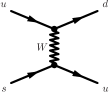
$\rightarrow$

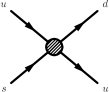
Figure 4: At low energies the single $W$ boson exchange reduces to a four-quark contact interaction.

2.3 Chiral symmetry in QCD

As mentioned above, the relevant symmetries of the underlying theory must also be maintained by the effective field theory. In this section, we will study the (approximate) chiral symmetry of QCD. The QCD Lagrangian reads in compact notation

$$\mathcal{L}_{\mbox{\scriptsize{QCD}}}=\bar{q}\left(i\gamma^{\mu}D_{\mu}-m_{q}\right)q-\frac{1}{2}\mbox{Tr}_{c}\left(G^{\mu\nu}G_{\mu\nu}\right)\ ,$$ (8)

where $q^{T}=(u,d,s,c,b,t)$ comprises the six quark flavors, $D_{\mu}=\partial_{\mu}-igG_{\mu}$ is the covariant derivative, $G_{\mu}$ the gluon fields, and $G_{\mu\nu}=\partial_{\mu}G_{\nu}-\partial_{\nu}G_{\mu}-ig\,[G_{\mu},G_{\nu}]$ the gluon field strength tensor. Tr_c denotes the trace in color space. The Dirac field $q$ is a 72-component object; each of the 6 quark flavors appears in 3 different colors and has 4 spinor components.

The quarks can be grouped into light and heavy flavors according to their masses: the $u,d,s$ quarks are substantially lighter than the $c,b,t$ quarks pdg . Hence, the limit of massless light quarks, $m_{u}=m_{d}=m_{s}=0$, the so-called chiral limit, seems to be a reasonable approximation and can be improved by treating the light quark masses as perturbations. The $c,b,t$ quarks, on the other hand, can be treated at low energies as infinitely heavy and the only active degrees of freedom are those associated with the light $u,d,s$ quarks.

It is straightforward to see that in the chiral limit the QCD Lagrangian has an extra symmetry. In this limit, the relevant part of $\mathcal{L}_{\mbox{\scriptsize{QCD}}}$ is (we use the same notation for simplicity)

$$\mathcal{L}_{\mbox{\scriptsize{QCD}}}=\sum_{q=u,d,s}\bar{q}i\gamma_{\mu}D^{\mu}q-\frac{1}{2}\mbox{Tr}_{c}(G_{\mu\nu}G^{\mu\nu})\ .$$ (9)

Here, $q$ represents a one-flavor quark field. By introducing right- and left-handed quark fields

$$q_{R/L}=\,\frac{1}{2}(1\pm\gamma_{5})\,q$$ (10)

one arrives at

$$\mathcal{L}_{\mbox{\scriptsize{QCD}}}=\sum_{q=u,d,s}\left(\bar{q}_{L}i\gamma_{\mu}D^{\mu}q_{L}+\bar{q}_{R}i\gamma_{\mu}D^{\mu}q_{R}\right)-\frac{1}{2}\mbox{Tr}_{c}(G_{\mu\nu}G^{\mu\nu})\ .$$ (11)

Independent transformations of the right- and left-handed quark fields

$$q_{R}\,\rightarrow\,R\,q_{R}\ ,\qquad\qquad q_{L}\,\rightarrow\,L\,q_{L}$$ (12)

with $R\in\mbox{SU(3)}_{R},\ L\in\mbox{SU(3)}_{L}$ leave the massless QCD Lagrangian invariant. This invariance is referred to as SU(3)${}_{L}\times$SU(3)_R chiral symmetry of massless QCD. One observes that the gluon interactions do not change the helicity of quarks but the quark mass term does.

Due to Noether’s theorem an immediate consequence of a continuous symmetry of a Lagrangian is the existence of a conserved current $J_{\mu}$ with $\partial_{\mu}J^{\mu}=0$. The corresponding charge

$$Q(t)=\int d^{3}x\ J_{0}(t,\mathbf{x})$$ (13)

is time-independent, i.e. $dQ/dt=0$. Familiar examples are the invariance of the Lagrangian with regard to translations in time and space and rotations which imply, respectively, conservation of energy, momentum and angular momentum. At the operator level, the conserved charges commute with the Hamiltonian.

In the chiral limit of QCD the conserved currents of chiral symmetry are

$$L_{\mu}^{a}=\sum_{q=u,d,s}\bar{q}_{L}\gamma_{\mu}\frac{\lambda^{a}}{2}q_{L}\ ,\qquad\quad R_{\mu}^{a}=\sum_{q=u,d,s}\bar{q}_{R}\gamma_{\mu}\frac{\lambda^{a}}{2}q_{R}$$ (14)

with the Gell-Mann matrices $\lambda^{a}$. The invariant charges $Q_{L}^{a},Q_{R}^{a}$ generate the algebra of SU(3)_L and SU(3)_R, respectively. It is useful to define the combinations

$$Q_{V}^{a}=Q_{R}^{a}+Q_{L}^{a}\ ;\qquad Q_{A}^{a}=Q_{R}^{a}-Q_{L}^{a}$$ (15)

which have a different behavior under parity

$$Q_{V}^{a}\rightarrow Q_{V}^{a}\ ;\qquad Q_{A}^{a}\rightarrow-Q_{A}^{a}\ .$$ (16)

Consider an eigenstate $|\psi\rangle$ of $H_{\mbox{\scriptsize{QCD}}}$ (in the chiral limit)

$$H_{\mbox{\scriptsize{QCD}}}|\psi\rangle=E|\psi\rangle\ .$$ (17)

The states $Q_{V}^{a}|\psi\rangle$ and $Q_{A}^{a}|\psi\rangle$ have the same energy $E$ but opposite parity. Thus for each positive parity state there should be a negative parity state with equal mass. This pattern is, however, not observed in the particle spectrum pdg . For example, the light pseudoscalar ($J^{P}=0^{-}$) mesons, $(\pi,K,\eta)$, have a considerably lower mass than the scalar ($J^{P}=0^{+}$) mesons.

The solution to this paradoxon is provided by the Nambu-Goldstone realization of chiral symmetry NJL which asserts that the QCD vacuum, $|0\rangle$, is not invariant under the action of the axial charges

$$Q_{V}^{a}|0\rangle=0\qquad Q_{A}^{a}|0\rangle\neq 0\ .$$ (18)

The chiral $SU(3)_{L}\times SU(3)_{R}$ symmetry of the QCD Hamiltonian is said to be spontaneously broken down to $SU(3)_{V}$. Spontaneous breakdown of a symmetry takes place if the full symmetry group of the Hamiltonian is not shared by the vacuum.

Another example of spontaneous symmetry breakdown occurs in ferromagnets. For temperatures above the Curie temperature, $T>T_{c}$, the magnetic dipoles are randomly oriented. As soon as the temperature falls below the Curie temperature $T_{c}$ spontaneous magnetization occurs and the dipoles are aligned in some arbitrary direction. Spontaneous symmetry breakdown takes also place for the SU(2)${}_{L}\times$U(1) symmetry of the electroweak interactions.

In general, spontaneous breakdown of a continuous symmetry has important consequences. Goldstone’s theorem states that a spontaneously broken continuous symmetry implies massless spinless particles: the Goldstone bosons. In the case of massless QCD, the eight axial charges $Q_{A}^{a}$ create states $|\phi\rangle=Q_{A}|0\rangle$ which are energetically degenerate with the vacuum $|0\rangle$ since

$$H|\phi\rangle=HQ_{A}|0\rangle=Q_{A}H|0\rangle=0\ .$$ (19)

This gives rise to eight massless pseudoscalar mesons. The axial charges $Q_{A}^{a}$ acting on any particle state generate Goldstone bosons, e.g. an energy eigenstate $|\psi\rangle$ is degenerate with the multi-particle state $Q_{A}^{a}|\psi\rangle$ which resolves the paradoxon from above.

The eight lightest hadrons are indeed the pseudoscalars $\pi^{\pm}$,$\pi^{0}$,$K^{\pm}$,$K^{0}$,$\bar{K}^{0}$,
$\eta$ with masses $m_{\pi}\approx 138$ MeV, $m_{K}\approx 495$ MeV and $m_{\eta}\approx 547$ MeV pdg . Since the nonzero masses of the light quarks break chiral symmetry explicitly the Goldstone bosons are not exactly massless. However, the explicit breaking can be considered to be small and treated perturbatively. In the limit of vanishing quark masses, $m_{u},m_{d},m_{s}\rightarrow 0$, the Goldstone boson masses approach zero, $m_{\pi},m_{K},m_{\eta}\rightarrow 0$, while all other hadrons remain massive in the chiral limit and are separated from the ground state roughly by a characteristic gap

$$\Delta\sim M_{\mbox{\scriptsize proton}}\sim 1\,\mbox{GeV}\ .$$ (20)

In the remainder of this section, it is demonstrated that only the spontaneous breakdown of a continuous symmetry gives rise to Goldstone bosons, whereas in the case of a discrete symmetry Goldstone bosons are not generated.

Discrete symmetry case

Consider the Lagrangian density with a scalar field $\phi$

$$\mathcal{L}=\frac{1}{2}\partial_{\mu}\phi\partial^{\mu}\phi+\frac{1}{2}m^{2}\phi^{2}-\frac{1}{4}\lambda\phi^{4}\ .$$ (21)

The Lagrangian is invariant under the discrete symmetry of reflections, $\phi\rightarrow-\phi$. The corresponding potential is given by

$$V(\phi^{2})=-\frac{1}{2}m^{2}\phi^{2}+\frac{1}{4}\lambda\phi^{4}\ ,$$ (22)

and since the energy must be bound from below the coupling $\lambda$ is positive. The coefficient $m^{2}$, on the other hand, is not constrained. There are two possible cases depending on the sign of $m^{2}$ as illustrated in Fig. 5.

\begin{overpic}[width=86.72267pt,clip]{nobreak.eps} \put(90.0,-10.0){\scalebox{0.9}{$\phi$}} \put(52.0,58.0){\scalebox{0.9}{$V(\phi^{2})$}} \end{overpic}

\begin{overpic}[width=86.72267pt,clip]{break.eps} \put(92.0,13.0){\scalebox{0.9}{$\phi$}} \put(52.0,58.0){\scalebox{0.9}{$V(\phi^{2})$}} \end{overpic}

Figure 5: Potential $V(\phi^{2})$, Eq. (22), for $m^{2}<0$ (left) and $m^{2}>0$ (right).

For $m^{2}<0$ there is a unique minimum at $\phi=0$, but for $m^{2}>0$ the potential $V(\phi^{2})$ is minimized by two possible ground state fields $\phi=\pm\sqrt{m^{2}/\lambda}$. In the quantum field theoretical language this implies that the field $\phi$ develops a vacuum expectation value

$$\langle 0|\phi|0\rangle=\pm\sqrt{\frac{m^{2}}{\lambda}}\ .$$ (23)

Hence, there are two possible vacua but each vacuum is not invariant under reflection symmetry, i.e. the theory is spontaneously broken. Massless Goldstone bosons, however, do not appear.

Continuous symmetry case

Consider now the Lagrangian with two scalar fields $\sigma$ and $\pi$

$$\mathcal{L}=\frac{1}{2}(\partial_{\mu}\sigma)^{2}+\frac{1}{2}(\partial_{\mu}\pi)^{2}-V(\sigma^{2}+\pi^{2})$$ (24)

with $V$ defined as in Eq. (22). It exhibits an O(2) symmetry; continuous transformations of the type

$$\left(\begin{array}[]{c}\sigma\\ \pi\end{array}\right)\rightarrow\left(\begin{array}[]{cc}\phantom{+}\cos\alpha&\phantom{+}\sin\alpha\\ -\sin\alpha&\phantom{+}\cos\alpha\end{array}\right)\left(\begin{array}[]{c}\sigma\\ \pi\end{array}\right)$$ (25)

leave the Lagrangian invariant. The extrema of the corresponding potential $V$ are determined by the equations

$$\frac{dV}{d\sigma} = \sigma[-m^{2}+\lambda(\sigma^{2}+\pi^{2})]=0\ ,$$

$$\frac{dV}{d\pi} = \pi[-m^{2}+\lambda(\sigma^{2}+\pi^{2})]=0\ .$$ (26)

For $m^{2}>0$ the minima are at $\sigma^{2}+\pi^{2}=m^{2}/\lambda$ and related to each other through O(2) rotations. Any point on the circle of minima may be chosen to be the true vacuum $|0\rangle$. One may take, e.g.,

$$\langle 0|\sigma|0\rangle=\sqrt{\frac{m^{2}}{\lambda}}\ ;\qquad\langle 0|\pi|0\rangle=0\ .$$ (27)

Clearly, the O(2) symmetry of the Lagrangian is spontaneously broken by the vacuum state. Small oscillations around this vacuum state can be described by shifting the $\sigma$ field

$$\sigma^{\prime}\equiv\sigma-\sqrt{\frac{m^{2}}{\lambda}}$$ (28)

so that the Lagragian reads in terms of the new fields (up to an irrelevant constant)

$$\mathcal{L} = \,\frac{1}{2}(\partial_{\mu}\sigma^{\prime})^{2}+\frac{1}{2}(\partial_{\mu}\pi)^{2}-m^{2}\sigma^{\prime 2}$$ (29)

$$-\lambda\,\sqrt{\frac{m^{2}}{\lambda}}\,\sigma^{\prime}\,(\sigma^{\prime 2}+\pi^{2})-\frac{1}{4}\,\lambda\,(\sigma^{\prime 2}+\pi^{2})^{2}\ .$$

With this choice of coordinates the mass term for the $\pi$ field has disappeared and the $\pi$ becomes massless. The $\pi$ field is then interpreted as a polar angle oscillation around the vacuum which does not cost any energy. A Goldstone boson has been created through spontaneous breakdown of the continuous O(2) symmetry in the original Lagrangian.

3 Construction of the chiral effective Lagrangian

In this section we outline the construction principles for the chiral effective Lagrangian. The chiral SU(3) Lagrangian is in general a function of the Goldstone boson (GB) fields $(\pi^{0},\pi^{\pm},K^{\pm},K^{0},\bar{K}^{0},\eta)$. In order to construct the effective Lagrangian, we must first know the interaction between the GBs.

To this aim, we recall from the previous section that the eight axial charges $Q_{A}^{a}$ do not annihilate the vacuum, $Q_{A}^{a}|0\rangle\neq 0$. The states $Q_{A}^{a}|0\rangle\neq 0$ are associated with the GBs $\phi^{a}=(\pi,K,\eta)$. This implies non-vanishing matrix elements of the axial vector current $A_{\mu}^{a}$

$$\langle 0|A_{\mu}^{a}(x)|\phi^{b}(p)\rangle=ie^{-ip\cdot x}\,p_{\mu}\,\delta^{ab}\,f_{a}$$ (30)

(no summation over $a$). The decay constant $f_{a}$ measures the strength with which the Goldstone boson $\phi^{a}$ decays via the axial vector current $A_{\mu}^{a}$ into the hadronic vacuum. The decay constants are extracted experimentally from weak decays of the GBs, e.g., $\pi^{+}\to l^{+}\nu_{l}$ yields $f_{\pi}=92.4$ MeV Hol .

Taking the divergence of Eq. (30) leads to

$$\langle 0|\partial^{\mu}A_{\mu}^{a}(0)|\phi^{b}(p)\rangle=\delta^{ab}m_{a}^{2}f_{a}\ .$$ (31)

In the chiral limit, the axial vector current is conserved, $\partial^{\mu}A_{\mu}^{a}=0$, so that $m_{a}^{2}=0$ as required by Goldstone’s theorem. In the real world, however, chiral SU(3)${}_{L}\times$ SU(3)_R symmetry is explicitly broken by the finite quark masses $m_{u},m_{d},m_{s}$ and the axial vector current is not conserved. One introduces the GB field operators $\Phi^{a}$ with the normalization $\langle 0|\Phi^{a}(0)|\phi^{b}(p)\rangle=\delta^{ab}$. Eq. (31) can then be rewritten as

$$\langle 0|\partial^{\mu}A_{\mu}^{a}(0)|\phi^{b}(p)\rangle=m_{a}^{2}f_{a}\langle 0|\Phi^{a}(0)|\phi^{b}(p)\rangle\ .$$ (32)

At the operator level, this is the hypothesis of the partially conserved axial vector current (PCAC)

$$\partial^{\mu}A_{\mu}^{a}=m_{a}^{2}f_{a}\Phi^{a}\ .$$ (33)

The axial currents can thus be employed as interpolating fields for the Goldstone bosons and identity (33) implies a vanishing interaction between the GBs at zero momentum. Consider to this end, e.g., the matrix element (suppressing flavor indices)

$${\cal M}_{\mu}(p_{1},p_{2},p_{3})=\langle\phi(p_{2})\phi(p_{3})|A_{\mu}(0)|\phi(p_{1})\rangle\ .$$ (34)

The amplitude ${\cal M}_{\mu}$ contains two parts: contributions with no GB poles and contributions where the axial current generates a GB pole, see Fig. 6.

Figure 6: Contributions to ${\cal M}_{\mu}$ in Eq. (34) with (left) and without (right) a GB pole. The wavy and solid lines denote the axial vector current and the Goldstone bosons, respectively.

In the chiral limit, the matrix element has the decomposition

$${\cal M}_{\mu}(p_{1},p_{2},p_{3})=\frac{fq_{\mu}}{q^{2}}T(p_{1},p_{2},p_{3},q)+R_{\mu}\ ,$$ (35)

where $q=-p_{1}-p_{2}-p_{3}$, $T$ is the GB-GB scattering matrix element, $f$ the decay constant in the chiral limit, and $R_{\mu}$ is non-singular as $q_{\mu}\to 0$ by definition. Contracting both sides with $q^{\mu}$ yields

$$0=q^{\mu}{\cal M}_{\mu}(p_{1},p_{2},p_{3})=fT(p_{1},p_{2},p_{3},q)+q^{\mu}R_{\mu}\ .$$ (36)

In the limit $q_{\mu}\to 0$ one obtains

$$T(p_{1},p_{2},p_{3},q)=0\ .$$ (37)

The GBs do not interact at vanishing momenta.

At low but finite energies, the interaction between GBs can be expanded in powers of small momenta. Consider for example the GB-GB scattering matrix $T$ which can be written as a function of the three Mandelstam variables $s=(p_{1}+p_{2})^{2}$, $t=(p_{1}+p_{3})^{2}$ and $u=(p_{1}+q)^{2}$. Its low energy expansion reads

$$T(s,t,u)=f_{1}s+g_{1}t+h_{1}u+\ldots$$ (38)

with momentum-independent expansion coefficients $f_{i},g_{i},h_{i}$. The chiral effective Lagrangian is also ordered according to the low energy expansion. Powers of GB momenta in the amplitude correspond to powers of derivatives on GB fields in the Lagrangian. The ordering of the effective Lagrangian in increasing powers of derivatives is called chiral ordering or chiral power counting.

Next, we would like to investigate how GB fields are represented in the chiral Lagrangian. To this aim, we shall study the transformation properties of the GBs under chiral transformations.

Let $G$ be the group of chiral SU(3)${}_{L}\times$ SU(3)_R transformations. For a given representation of $G$ the GB fields transform according to

$$\phi\to\phi^{\prime}=F(g,\phi)\ ,\qquad g\in G$$ (39)

with the representation property

$$F(g_{1},F(g_{2},\phi))=F(g_{1}g_{2},\phi)\ .$$ (40)

Consider group elements $h\in G$ which leave the “origin”, i.e. the vacuum, invariant, $F(h,0)=0$. Obviously, these elements form a subgroup $H$: for $h_{1},h_{2}\in H$ it follows that $h_{1}h_{2}\in H$. $H$ is equivalent to the subgroup SU(3)_V which leaves the vacuum invariant.

The function

$$g\to F(g,0)=F(gh,0)\qquad h\in H$$ (41)

maps the coset space $G/H$ onto the space of GB fields. This mapping is invertible since $F(g_{1},0)=F(g_{2},0)$ implies $g_{1}^{-1}g_{2}\in H$. As the dimension of the coset space is equal to the number of Goldstone boson fields, the GBs can be identified with elements of $G/H$. The Goldstone boson fields are said to live on the coset space SU(3)${}_{L}\times$ SU(3)_R/SU(3)_V.

Any $g\in G$ can be decomposed as $g=qh$ with $q\in G/H$ and $h\in H$. The choice of representatives in the coset space $G/H$ is arbitrary. Possible choices are for example

$$g=(g_{L},g_{R})=(1,g_{R}g_{L}^{-1})(g_{L},g_{L})\equiv qh$$ (42)

or

$$g=(g_{L},g_{R})=(g_{L}g_{R}^{-1},1)(g_{R},g_{R})\equiv q^{\prime}h^{\prime}\ .$$ (43)

If we pick, e.g., the latter choice then the action of $G$ on $G/H$ is given by

$$(L,R)(g_{L}g_{R}^{-1},1)=(Lg_{L}g_{R}^{-1},R)=(Lg_{L}g_{R}^{-1}R^{-1},1)(R,R)\ .$$ (44)

The Goldstone bosons are then summarized by the matrix-valued field $U=g_{L}g_{R}^{-1}$ which transforms under chiral transformations as

$$U(x)\to U^{\prime}(x)=LU(x)R^{-1}=LU(x)R^{\dagger}$$ (45)

for $L/R\in\mbox{SU(3)}_{L/R}$. The exponential representation is convenient for $U\in$ SU(3)

$$U=\exp\left(\frac{i}{f}\phi^{a}\lambda^{a}\right)\ ,$$ (46)

where $\lambda^{a}$ are the generators of SU(3)

$$\phi=\phi^{a}\lambda^{a}=\sqrt{2}\left(\begin{array}[]{ccc}\frac{1}{\sqrt{2}}\pi^{0}+\frac{1}{\sqrt{6}}\eta&\phantom{+}\pi^{+}&\phantom{+}K^{+}\\ \phantom{+}\pi^{-}&-\frac{1}{\sqrt{2}}\pi^{0}+\frac{1}{\sqrt{6}}\eta&\phantom{+}K^{0}\\ \phantom{+}K^{-}&\phantom{+}\bar{K}^{0}&\phantom{+}-\frac{2}{\sqrt{6}}\eta\end{array}\right)\ .$$ (47)

The chiral effective Lagrangian for QCD is written in terms of the GB fields which are collected in the matrix-valued field $U$

$$\mathcal{L}_{\mbox{\scriptsize{eff}}}=\mathcal{L}_{\mbox{\scriptsize{eff}}}(U,\partial U,\partial^{2}U,\ldots)\ .$$ (48)

The effective Lagrangian shares the same symmetries with QCD: $C,P,T$, Lorentz invariance and, in particular, chiral SU(3)${}_{L}\times$ SU(3)_R symmetry. As outlined above, the chiral Lagrangian is expanded in chiral powers which are related (in the chiral limit) to the number of derivatives acting on the GB fields. The chiral power counting of the Lagrangian reads

$$\mathcal{L}_{\mbox{\scriptsize{eff}}}=\mathcal{L}_{\mbox{\scriptsize{eff}}}^{(0)}+\mathcal{L}_{\mbox{\scriptsize{eff}}}^{(2)}+\mathcal{L}_{\mbox{\scriptsize{eff}}}^{(4)}+\ldots\ .$$ (49)

Only even chiral powers arise since the Lagrangian is a Lorentz scalar which implies that tensor indices of derivatives appear in pairs. At each chiral order the effective Lagrangian must be invariant under chiral SU(3)${}_{L}\times$ SU(3)_R transformations. At zeroth chiral order this invariance implies that $\mathcal{L}_{\mbox{\scriptsize{eff}}}^{(0)}$ can only be a function of $UU^{\dagger}=1$. This amounts to an irrelevant constant in the Lagrangian which can be dropped.

At second order, the chiral invariant terms with two derivatives are

$$\mathcal{L}_{\mbox{\scriptsize{eff}}}^{(2)}=c_{1}\langle\partial_{\mu}U^{\dagger}\partial^{\mu}U\rangle+c_{2}\langle U^{\dagger}\Box U\rangle\ ,$$ (50)

where $\langle\ldots\rangle$ is the trace in flavor space. The second term can be reduced to the first one by partial integration; only one term remains at second chiral order

$$\mathcal{L}_{\mbox{\scriptsize{eff}}}^{(2)}=c_{1}\langle\partial_{\mu}U^{\dagger}\partial^{\mu}U\rangle\ .$$ (51)

Since terms of zeroth chiral order have been dropped, the second chiral order is effectively the leading order (LO). We note the appearance of a coupling constant $c_{1}$, a so-called low-energy constant (LEC). It is fixed by expanding the matrix-valued field $U$ in the GB fields $\phi$

$$U=\exp\left(\frac{i}{f}\phi\right)=1+\frac{i}{f}\phi-\frac{1}{2f^{2}}\phi^{2}+{\cal O}(\phi^{3})$$ (52)

and requiring the standard kinetic term

$$\mathcal{L}_{\mbox{\scriptsize{eff}}}^{(2)}=\frac{1}{2}\partial_{\mu}\phi^{a}\partial^{\mu}\phi^{a}+{\cal O}(\phi^{4})$$ (53)

which yields $c_{1}=f^{2}/4$.

Therefore, the effective Lagrangian at LO reads

$$\mathcal{L}_{\mbox{\scriptsize{eff}}}^{(2)}=\frac{f^{2}}{4}\langle\partial_{\mu}U^{\dagger}\partial^{\mu}U\rangle\ .$$ (54)

At leading chiral order there is only one LEC (in the chiral limit) and chiral symmetry constrains all vertices with increasing number of GB fields in the LO Lagrangian.

The interpretation of the LEC $f$ can be directly inferred by considering the Noether axial current of chiral symmetry for $\mathcal{L}_{\mbox{\scriptsize{eff}}}^{(2)}$

$$A_{\mu}^{a}=i\frac{f^{2}}{4}\langle\lambda^{a}\{\partial_{\mu}U,U^{\dagger}\}\rangle\ .$$ (55)

Upon comparison with the PCAC hypothesis

$$\langle 0|A_{\mu}^{a}(0)|\phi^{b}(p)\rangle=ip_{\mu}\delta^{ab}f_{a}$$ (56)

one confirms that $f$ is the GB decay constant in the chiral limit.

As a first application we are now in a position to predict, e.g., $\pi\pi$ scattering at leading chiral order. The scattering amplitude has the decomposition

$${\cal M}(\pi^{a}(p_{a})\,\pi^{b}(p_{b})\to\pi^{c}(p_{c})\,\pi^{d}(p_{d}))$$

$$\quad=\delta^{ab}\delta^{cd}A(s,t,u)+\delta^{ac}\delta^{bd}A(t,s,u)+\delta^{ad}\delta^{bc}A(u,t,s)\ ,$$ (57)

where $a,b,c,d$ are flavor indices and $s=(p_{a}+p_{b})^{2},\,t=(p_{a}-p_{c})^{2},\,u=(p_{a}-p_{d})^{2}$. Employing $\mathcal{L}_{\mbox{\scriptsize{eff}}}^{(2)}$ one calculates

$$A(s,t,u)=\frac{s}{f^{2}}\ .$$ (58)

Up to now, we have worked in chiral limit $m_{u},m_{d},m_{s}=0$ where chiral symmetry is exact. In the real world the quark masses do not vanish and introduce an explicit breaking of chiral symmetry in $\mathcal{L}_{\mbox{\scriptsize{QCD}}}$

$$\mathcal{L}_{\mbox{\scriptsize{QCD}}}=\mathcal{L}_{\mbox{\scriptsize{QCD}}}^{0}-\bar{q}{\cal M}q=\mathcal{L}_{\mbox{\scriptsize{QCD}}}^{0}-\bar{q}_{R}{\cal M}q_{L}-\bar{q}_{L}{\cal M}q_{R}\ ,$$ (59)

where $\mathcal{L}_{\mbox{\scriptsize{QCD}}}^{0}$ is the massless QCD Lagrangian and ${\cal M}=\mbox{diag}(m_{u},m_{d},m_{s})$ the light quark mass matrix. The chiral symmetry breaking patterns induced by the light quark masses must be reproduced at the level of the effective field theory. To this end, we interpret the quark mass matrix as an external scalar source $s$

$$\bar{q}{\cal M}q=\bar{q}_{L}{\cal M}q_{R}+\bar{q}_{R}{\cal M}^{\dagger}q_{L}\to\bar{q}_{L}sq_{R}+\bar{q}_{R}s^{\dagger}q_{L}\ .$$ (60)

The external scalar source $s$ is required to transform under chiral rotations as

$$s\to LsR^{\dagger}\ .$$ (61)

Obviously, this leaves the QCD Lagrangian invariant under chiral rotations and implies that the effective Lagrangian must also remain invariant in the presence of $s$. Hence, the chiral invariant effective Lagrangian is extended with $s$ as an additional building block

$$\mathcal{L}_{\mbox{\scriptsize{eff}}}(U,\partial U,\partial^{2}U,\ldots)\to\mathcal{L}_{\mbox{\scriptsize{eff}}}(U,\partial U,\partial^{2}U,\ldots;s)\ .$$ (62)

Once the effective Lagrangian is constructed one can go back to the real world by setting $s={\cal M}$. In (standard) chiral perturbation theory the chiral counting rule is $s={\cal M}={\cal O}(p^{2})$, i.e. the quark masses are booked as second chiral order. In addition to the derivative expansion the effective Lagrangian is expanded in powers of $s$. At leading chiral order one obtains

$$\mathcal{L}_{\mbox{\scriptsize{eff}}}^{(2)} = \frac{f^{2}}{4}\langle\partial_{\mu}U^{\dagger}\partial^{\mu}U\rangle+\frac{f^{2}}{2}B\langle sU^{\dagger}+Us^{\dagger}\rangle$$ (63)

$$= \frac{f^{2}}{4}\langle\partial_{\mu}U^{\dagger}\partial^{\mu}U\rangle+\frac{f^{2}}{2}B\langle{\cal M}(U+U^{\dagger})\rangle\ .$$

We have introduced an additional constant $B$ related to explicit chiral symmetry breaking.

The expansion of the symmetry-breaking part in powers of GB fields reads

$$\frac{f^{2}}{2}B\langle{\cal M}(U+U^{\dagger})\rangle=(m_{u}+m_{d}+m_{s})Bf^{2}-\frac{1}{2}B\langle{\cal M}\phi^{2}\rangle+{\cal O}(\phi^{4})\ .$$ (64)

The first term in this expansion is related to the vacuum expectation values of the scalar quark densities

$$\langle 0|\bar{q}q|0\rangle=\langle 0|\frac{\textstyle\partial H_{\mbox{\tiny QCD}}}{\textstyle\partial m_{q}}|0\rangle=-\langle 0|\frac{\textstyle\partial\mathcal{L}_{\mbox{\tiny eff}}}{\textstyle\partial m_{q}}|0\rangle=-f^{2}B+{\cal O}(m_{q})$$ (65)

and $B$ is the order parameter of spontaneous chiral symmetry breaking. At lowest order the quark condensates are degenerate

$$\langle 0|\bar{u}u|0\rangle=\langle 0|\bar{d}d|0\rangle=\langle 0|\bar{s}s|0\rangle=-f^{2}B\ .$$ (66)

The second term in the expansion in Eq. (64) is the mass term for the GB fields

$$\begin{array}[]{ll}m^{2}_{\pi^{+}}&=2B\hat{m}\\ m^{2}_{\pi^{0}}&=2B\hat{m}+{\cal O}\left[\frac{\textstyle(m_{u}-m_{d})^{2}}{\textstyle m_{s}-\hat{m}}\right]\\ m^{2}_{K^{+}}&=B(m_{u}+m_{s})\\[5.69046pt] m^{2}_{K^{0}}&=B(m_{d}+m_{s})\\ m^{2}_{\eta}&=\frac{2}{3}B(\hat{m}+2m_{s})+{\cal O}\left[\frac{\textstyle(m_{u}-m_{d})^{2}}{\textstyle m_{s}-\hat{m}}\right]\end{array}$$ (67)

with $\hat{m}=\frac{1}{2}(m_{u}+m_{d})$. The terms proportional to $(m_{u}-m_{d})^{2}$ are due to $\pi^{0}$-$\eta$ mixing. They constitute tiny corrections and are usually neglected. The mass relations in Eq. (67) explain why one counts $s={\cal O}(p^{2})$ (taking $B$ to be of zeroth chiral order). For finite light quark masses we see that the GBs are not massless any longer (sometimes they are referred to as pseudo-GBs).

From the previous equalities one obtains immediately the Gell-Mann–Oakes–Renner relations

$$\begin{array}[]{ll}f_{\pi}^{2}m^{2}_{\pi}&=-2\hat{m}\langle 0|\bar{q}q|0\rangle+{\cal O}(m_{q}^{2})\\[5.69046pt] f_{K}^{2}m^{2}_{K}&=-(\hat{m}+m_{s})\langle 0|\bar{q}q|0\rangle+{\cal O}(m_{q}^{2})\\[5.69046pt] f_{\eta}^{2}m^{2}_{\eta}&=-\frac{2}{3}(\hat{m}+2m_{s})\langle 0|\bar{q}q|0\rangle+{\cal O}(m_{q}^{2})\\[5.69046pt] \end{array}$$ (68)

and the Gell-Mann–Okubo mass relation

$$3m^{2}_{\eta}=4m^{2}_{K}-m^{2}_{\pi}\ .$$ (69)

To leading chiral order, the strong interactions at low energies are characterized by the two scales $f$ and $B$ with

$$\begin{array}[]{rl}f\simeq f_{\pi}&\simeq 93\,\mathrm{MeV}\\[5.69046pt] B&\simeq 1800\,\mathrm{MeV}\ ,\end{array}$$ (70)

where the value of $B$ has been extracted from the sum-rule value $\langle 0|\bar{q}q|0\rangle=-(250\,\mathrm{MeV})^{3}$ SVZ .

One important goal of chiral perturbation theory is to extract the light quark mass ratios from phenomenology. Note that the absolute values of the quark masses cannot be extracted since they depend on the QCD renormalization scale, but the QCD scale dependence cancels out in quark mass ratios. For example, from the leading order mass relations one obtains

$$\frac{m_{u}}{m_{d}}=\frac{(m^{2}_{K^{+}}-m^{2}_{K^{0}})_{\mbox{\tiny QCD}}+m^{2}_{\pi^{0}}}{(m^{2}_{K^{0}}-m^{2}_{K^{+}})_{\mbox{\tiny QCD}}+m^{2}_{\pi^{0}}}\ ,$$ (71)

where the tiny contribution from $\pi^{0}$-$\eta$ mixing and electromagnetic effects in the kaon mass difference have been neglected. Next, we employ Dashen’s theorem Dash which asserts that electromagnetic contributions to the mass splittings $m^{2}_{K^{+}}-m^{2}_{K^{0}}$ and $m^{2}_{\pi^{+}}-m^{2}_{\pi^{0}}$ are identical in the chiral limit

$$\begin{array}[]{ll}(m^{2}_{K^{+}}-m^{2}_{K^{0}})_{\mbox{\scriptsize QCD}}&=(m^{2}_{K^{+}}-m^{2}_{K^{0}})_{\mbox{\scriptsize phys}}-(m^{2}_{K^{+}}-m^{2}_{K^{0}})_{\mbox{\scriptsize em}}\\[5.69046pt] &=(m^{2}_{K^{+}}-m^{2}_{K^{0}})_{\mbox{\scriptsize phys}}-(m^{2}_{\pi^{+}}-m^{2}_{\pi^{0}})_{\mbox{\scriptsize em}}\\[5.69046pt] &=(m^{2}_{K^{+}}-m^{2}_{K^{0}})_{\mbox{\scriptsize phys}}-(m^{2}_{\pi^{+}}-m^{2}_{\pi^{0}})_{\mbox{\scriptsize phys}}\ .\end{array}$$ (72)

The last equation is valid since the pion mass difference is (almost) entirely due to electromagnetic contributions. Insertion of this identity in the quark mass ratio yields Wei1

$$\frac{m_{u}}{m_{d}}=\frac{m^{2}_{K^{+}}-m^{2}_{K^{0}}+2m^{2}_{\pi^{0}}-m^{2}_{\pi^{+}}}{m^{2}_{K^{0}}-m^{2}_{K^{+}}+m^{2}_{\pi^{+}}}=0.55\ .$$ (73)

At leading order, the possibility $m_{u}=0$ which would lead to a solution of the strong $CP$ problem is excluded. In a similar manner one finds Wei1

$$\frac{m_{s}}{m_{d}}=\frac{m^{2}_{K^{0}}+m^{2}_{K^{+}}-m^{2}_{\pi^{0}}}{m^{2}_{K^{0}}-m^{2}_{K^{+}}+m^{2}_{\pi^{+}}}=20.1\ .$$ (74)

These leading order ratios are, of course, subject to higher order corrections.

We note in passing that due to the inclusion of finite quark masses the $\pi\pi$ scattering amplitude, Eq. (58), is modified according to

$$A(s,t,u)=\frac{s-m_{\pi}^{2}}{f^{2}}=\frac{s-m_{\pi}^{2}}{f^{2}_{\pi}}+{\cal O}(p^{4})\ .$$ (75)

In the remainder of this section we extend the effective field theoretical formalism to include external vector and axial-vector fields. This is necessary for the calculation of Green functions of quark currents, e.g., for the electromagnetic form factor of the pion

$$\langle\pi(p^{\prime})|J_{\mu}^{\mbox{\scriptsize{em}}}|\pi(p)\rangle=\langle\pi(p^{\prime})|\bar{q}\gamma_{\mu}Qq|\pi(p)\rangle\ ,$$ (76)

where $Q=\frac{1}{3}\mbox{diag}(2,-1,-1)$ is the quark charge matrix. Green functions of quark currents are conveniently calculated by applying the external field method. (As a matter of fact, we have already encountered this technique for the scalar quark densities $\langle 0|\bar{q}q|0\rangle$ which are obtained by differentiating with respect to the external field $s$.)

To this aim, one extends $\mathcal{L}_{\mbox{\scriptsize{QCD}}}$ in the presence of external fields

$$\mathcal{L}_{\mbox{\scriptsize{QCD}}}=\mathcal{L}_{\mbox{\scriptsize{QCD}}}^{0}+\bar{q}\gamma_{\mu}(v^{\mu}+\gamma_{5}a^{\mu})q-\bar{q}(s+i\gamma_{5}p)q\ ,$$ (77)

where $v^{\mu}$, $a^{\mu}$, $s$, and $p$ are hermitian matrices denoting the external vector, axial-vector, scalar, and pseudoscalar fields, respectively. The coupling of external photon fields ${\cal A}_{\mu}$ to the quarks, e.g., is given by the prescription $v_{\mu}=-eQ{\cal A}_{\mu}$. Green functions of electromagnetic currents are then obtained by functional derivatives of the generating functional $Z[v,a,s,p]$ with respect to ${\cal A}_{\mu}$. Couplings to weak currents are also collected in $v_{\mu}$ and $a_{\mu}$.

Due to the inclusion of electromagnetic and weak currents global chiral symmetry is promoted to a local one. The Lagrangian $\mathcal{L}_{\mbox{\scriptsize{QCD}}}$ in Eq. (77) remains invariant under the local chiral SU(3)${}_{L}\times$SU(3)_R transformations

$$\begin{array}[]{rl}q_{R}&\to\ Rq_{R}\\[5.69046pt] q_{L}&\to\ Lq_{L}\\[5.69046pt] r_{\mu}=v_{\mu}+a_{\mu}&\to\ Rr_{\mu}R^{\dagger}+iR\partial_{\mu}R^{\dagger}\\[5.69046pt] l_{\mu}=v_{\mu}-a_{\mu}&\to\ Ll_{\mu}L^{\dagger}+iL\partial_{\mu}L^{\dagger}\\[5.69046pt] s+ip&\to\ L(s+ip)R^{\dagger}\ .\end{array}$$ (78)

Local chiral symmetry must also be maintained by the extended effective Lagrangian in the presence of external fields

$$\mathcal{L}_{\mbox{\scriptsize{eff}}}(U,\partial U,\partial^{2}U,\ldots)\to\mathcal{L}_{\mbox{\scriptsize{eff}}}(U,\partial U,\partial^{2}U,\ldots;v,a,s,p)\ .$$ (79)

The local nature of chiral symmetry requires the introduction of a covariant derivative

$$\partial_{\mu}U\to D_{\mu}U=\partial_{\mu}U-il_{\mu}U+iUr_{\mu}$$ (80)

which transforms under chiral rotations as

$$D_{\mu}U\to L(D_{\mu}U)R^{\dagger}\ .$$ (81)

In addition, the vector and axial-vector fields $v_{\mu}$, $a_{\mu}$ enter the effective Lagrangian also through the non-Abelian field strength tensors, $R_{\mu\nu},L_{\mu\nu}$,

$$\begin{array}[]{l}R_{\mu\nu}=\partial_{\mu}r_{\nu}-\partial_{\nu}r_{\mu}-i[r_{\mu},r_{\nu}]\\[5.69046pt] L_{\mu\nu}=\partial_{\mu}l_{\nu}-\partial_{\nu}l_{\mu}-i[l_{\mu},l_{\nu}]\end{array}$$ (82)

with the transformation properties

$$R_{\mu\nu}\to R\,R_{\mu\nu}\,R^{\dagger}\ ,\qquad L_{\mu\nu}\to L\,L_{\mu\nu}\,L^{\dagger}\ .$$ (83)

4 Higher orders and loops

In the previous section we have outlined the construction principles for the chiral effective Lagrangian. The effective Lagrangian is ordered in powers of Goldstone boson momenta and masses, a chiral power counting scheme is established. The leading order effective Lagrangian $\mathcal{L}_{\mbox{\scriptsize{eff}}}^{(2)}$ was constructed explicitly and sample calculations have been performed at the leading tree level order. In this section we focus on the inclusion of next-to-leading order (NLO) contributions. On the one hand, these are the tree level diagrams with vertices from $\mathcal{L}_{\mbox{\scriptsize{eff}}}^{(4)}$. On the other hand, loop diagrams with vertices from $\mathcal{L}_{\mbox{\scriptsize{eff}}}^{(2)}$ must be taken into account.

The chiral expansion of the effective Lagrangian reads

$$\mathcal{L}_{\mbox{\scriptsize{eff}}}=\mathcal{L}_{\mbox{\scriptsize{eff}}}^{(2)}+\mathcal{L}_{\mbox{\scriptsize{eff}}}^{(4)}+\ldots\ .$$ (84)

The most general effective Lagrangian at fourth chiral order, $\mathcal{L}_{\mbox{\scriptsize{eff}}}^{(4)}$, which respects the relevant symmetries of QCD is GL2

$$\begin{array}[]{ll}\mathcal{L}_{\mbox{\scriptsize{eff}}}^{(4)}&=L_{1}\langle D_{\mu}U^{\dagger}D^{\mu}U\rangle^{2}+L_{2}\langle D_{\mu}U^{\dagger}D_{\nu}U\rangle\langle D^{\mu}U^{\dagger}D^{\nu}U\rangle\\[5.69046pt] &+\,L_{3}\langle D_{\mu}U^{\dagger}D^{\mu}UD_{\nu}U^{\dagger}D^{\nu}U\rangle+L_{4}\langle D_{\mu}U^{\dagger}D^{\mu}U\rangle\langle\chi U^{\dagger}+U\chi^{\dagger}\rangle\\[5.69046pt] &+L_{5}\langle D_{\mu}U^{\dagger}D^{\mu}U(\chi^{\dagger}U+U^{\dagger}\chi)\rangle+L_{6}\langle\chi U^{\dagger}+U\chi^{\dagger}\rangle^{2}\\[5.69046pt] &+L_{7}\langle\chi U^{\dagger}-U\chi^{\dagger}\rangle^{2}+L_{8}\langle\chi U^{\dagger}\chi U^{\dagger}+U\chi^{\dagger}U\chi^{\dagger}\rangle\\[5.69046pt] &-iL_{9}\langle R^{\mu\nu}D_{\mu}U^{\dagger}D_{\nu}U+L^{\mu\nu}D_{\mu}UD_{\nu}U^{\dagger}\rangle+L_{10}\langle R_{\mu\nu}U^{\dagger}L^{\mu\nu}U\rangle\end{array}$$ (85)

with $\chi\equiv 2B(s+ip)$. Ten low-energy constants enter with unknown values which must be determined from phenomenology. At next-to-next-to-leading order even 90 unknown LECs enter BCE2 . Due to the proliferation of unknown couplings in the effective Lagrangian ChPT seems to lose its predictive power. However, the situation is ameliorated since only a few LECs contribute to a particular process. There is no need to determine all LECs of the effective Lagrangian for a given process. Moreover, the contributions from higher chiral orders are suppressed as they appear with additional powers of small momenta or Goldstone boson masses. Therefore in practice only the LECs from lower orders are required.

At fourth chiral order, contributions from $\mathcal{L}_{\mbox{\scriptsize{eff}}}^{(4)}$ to the pseudoscalar meson masses stem solely from tree diagrams, see Fig. 7.

Figure 7: Tree diagram contribution to the self-energy of the Goldstone bosons. The square denotes a vertex from $\mathcal{L}_{\mbox{\scriptsize{eff}}}^{(4)}$.

Corrections from $\mathcal{L}_{\mbox{\scriptsize{eff}}}^{(4)}$ to $\pi\pi$ scattering at ${\cal O}(p^{4})$ also contribute through tree diagrams, Fig. 8.

Figure 8: Tree diagram contribution to $\pi\pi$ scattering at order order ${\cal O}(p^{4})$. The square denotes a vertex from $\mathcal{L}_{\mbox{\scriptsize{eff}}}^{(4)}$.

As already indicated above, tree diagrams are not the whole story. At next-to-leading order loop diagrams must be included as well. The loops also restore unitarity of the $S$-matrix which can be seen as follows. Unitarity of the $S$-matrix implies

$$SS^{\dagger}=1\ .$$ (86)

Inserting the usual decomposition $S=1+iT$ yields

$$-i(T-T^{\dagger})=T^{\dagger}T\ .$$ (87)

Since $T$ is symmetric due to time reversal invariance the last relation simplifies to

$$2\,\mbox{Im}\,T=T^{\dagger}T\ .$$ (88)

Tree diagrams do not have an imaginary piece and thus cannot satisfy Eq. (88), i.e., unitarity is violated if only tree diagrams are taken into account. However, unitarity of the $S$-matrix is perturbatively restored by including loop diagrams which have imaginary parts.

As a simple example of a loop calculation, we sketch the evaluation of the one-loop contributions to the GB self-energies. To this end, we expand the $U$ fields in $\mathcal{L}_{\mbox{\scriptsize{eff}}}^{(2)}$

$$\begin{array}[]{ll}\mathcal{L}_{\mbox{\scriptsize{eff}}}^{(2)}&=\frac{f^{2}}{4}\langle D_{\mu}U^{\dagger}D^{\mu}U\rangle+\frac{f^{2}}{2}B\langle{\cal M}(U^{\dagger}+U)\rangle\\[5.69046pt] &=\mathcal{L}_{\mbox{\scriptsize{kin}}}+\mathcal{L}_{\mbox{\scriptsize{int}}}\\[5.69046pt] &=\frac{1}{4}\langle\partial_{\mu}\phi\partial^{\mu}\phi\rangle-\frac{1}{2}B\langle{\cal M}\phi^{2}\rangle\\[5.69046pt] &\quad+\frac{1}{48f^{2}}\langle[\partial_{\mu}\phi,\phi][\partial^{\mu}\phi,\phi]\rangle+\frac{1}{24f^{2}}B\langle{\cal M}\phi^{4}\rangle+\ldots\quad.\end{array}$$ (89)

Interaction vertices with four GB fields arise which yield contributions to the meson masses via tadpoles, see Fig. 9.

Figure 9: Tadpole contribution to the self-energy of the Goldstone bosons. The vertex stems from $\mathcal{L}_{\mbox{\scriptsize{eff}}}^{(2)}$.

The calculation of the tadpole diagram involves the loop integration

$$\int\frac{d^{4}k}{(2\pi)^{4}}\frac{i}{k^{2}-m_{\phi}^{2}+i\epsilon}\ ,$$ (90)

where $m_{\phi}$ is the GB mass in the loop. This loop integral is quadratically ultraviolet divergent and a regularization scheme is necessary which maintains the symmetries of the theory, in particular chiral symmetry. One must be careful when employing cutoff regularization schemes since these introduce an additional massive cutoff scale which may spoil chiral symmetry GJLW . In this respect, a convenient mass-independent regularization scheme is provided by dimensional regularization. The basic idea of dimensional regularization is as follows. The dimension of the loop integration is changed to an arbitrary dimension $d\in\mathds{R}$. For $d$ small enough the integral remains ultraviolet finite and can be performed explicitly. Afterwards, the analytic continuation back to $d=4$ dimensions is performed.

To be more explicit, consider the tadpole integral in $d$ dimensions

$$I=\mu^{4-d}\int\frac{d^{d}k}{(2\pi)^{d}}\frac{i}{k^{2}-m_{\phi}^{2}+i\epsilon}\ .$$ (91)

The regularization scale $\mu$ has been introduced to maintain the mass dimension of $I$ for arbitrary space-time dimension $d$. The calculation of $I$ is performed in a straightforward manner

$$\begin{array}[]{ll}I&=\mu^{4-d}{\displaystyle\int\frac{d^{d}k}{(2\pi)^{d}}\frac{i}{k^{2}-m_{\phi}^{2}+i\epsilon}}={\displaystyle\mu^{4-d}\int\frac{d^{d}k_{\mbox{\tiny E}}}{(2\pi)^{d}}\frac{1}{k^{2}_{\mbox{\tiny E}}+m_{\phi}^{2}}}\\[11.38092pt] &={\displaystyle\mu^{4-d}\int\frac{d^{d}k_{\mbox{\tiny E}}}{(2\pi)^{d}}\int_{0}^{\infty}d\lambda\ \exp\left\{-\lambda\left(k^{2}_{\mbox{\tiny E}}+m_{\phi}^{2}\right)\right\}}\\[11.38092pt] &={\displaystyle\frac{\mu^{4-d}}{(2\pi)^{d}}\int_{0}^{\infty}d\lambda\ \exp\left(-\lambda m_{\phi}^{2}\right)\int d^{d}k_{\mbox{\tiny E}}\ \exp\left(-\lambda k^{2}_{\mbox{\tiny E}}\right)}\\[11.38092pt] &={\displaystyle\frac{\mu^{4-d}}{(2\pi)^{d}}\int_{0}^{\infty}d\lambda\ \exp\left(-\lambda m_{\phi}^{2}\right)\left(\frac{\pi}{\lambda}\right)^{d/2}}\\[11.38092pt] &={\displaystyle(4\pi)^{-\frac{d}{2}}m_{\phi}^{2}\left(\frac{m_{\phi}}{\mu}\right)^{d-4}\Gamma(1-\frac{d}{2})}\ .\end{array}$$ (92)

A Wick rotation to Euclidean space has been performed in the first line. Expanding the result in $d-4$ yields

$$I=m_{\phi}^{2}\left\{2L+\frac{1}{16\pi^{2}}\ln\left(\frac{m_{\phi}^{2}}{\mu^{2}}\right)\right\}+{\cal O}(d-4)$$ (93)

with the divergent piece

$$L=\frac{\mu^{d-4}}{16\pi^{2}}\left[\frac{1}{d-4}-\frac{1}{2}\left(\ln 4\pi+1+\Gamma^{\prime}(1)\right)\right]\ .$$ (94)

The tadpole integral $I$ is decomposed into two parts: a non-analytic term from the GB infrared singularities proportional to the “chiral log” $\ln(m_{\phi}^{2}/\mu^{2})$ and a piece $L$ which diverges for $d\to 4$.

A complete one-loop calculation for GB self-energies with vertices from $\mathcal{L}_{\mbox{\scriptsize{eff}}}^{(2)}$ reveals that divergent parts proportional to $L$ are of fourth chiral order and analytic in the quark masses and GB momenta. Hence, the divergent components can be compensated by renormalizing the LECs of fourth chiral order

$$L_{i}=L_{i}^{r}+\lambda_{i}L$$ (95)

such that the sum of loops and LECs (including fourth chiral order) remains finite for $d\to 4$ and can be evaluated in four space-time dimensions.

The above considerations for one-loop contributions to the self-energy can be generalized to other processes and higher loops. Consider a connected $L$-loop diagram for a given physical process. The chiral order (or chiral dimension) $D$ of a loop integral counts dimensions of GB masses and momenta (utilizing a mass-independent regularization scheme such as, e.g., dimensional regularization) and is given by

$$D=2+2L+\sum_{k}(k-2)N_{k}\ ,$$ (96)

where $L$ is the number of loops and $N_{k}$ the number of vertices of order ${\cal O}(p^{k})$.

Vertices from the lowest order Lagrangian $\mathcal{L}_{\mbox{\scriptsize{eff}}}^{(2)}$ do not alter the chiral dimension, while vertices from higher orders increase $D$. Each loop also increases the chiral dimension, i.e. the loopwise expansion corresponds with the chiral expansion. From Eq. (96) one infers that at leading chiral order only tree diagrams with vertices of $\mathcal{L}_{\mbox{\scriptsize{eff}}}^{(2)}$ contribute. At next-to-leading order both tree diagrams with exactly one fourth order vertex and one-loop diagrams with vertices of second chiral order contribute. Two-loop diagrams start contributing at sixth chiral order and so forth.

As an explicit example of the chiral expansion we consider the Feynman diagrams for $\pi\pi$ scattering up to one-loop order. At lowest order, ${\cal O}(p^{2})$, a tree diagram with a lowest order vertex contributes, see Fig. 10.

Figure 10: Leading ${\cal O}(p^{2})$ contribution to $\pi\pi$ scattering. The vertex stems from $\mathcal{L}_{\mbox{\scriptsize{eff}}}^{(2)}$.

At next-to-leading order, ${\cal O}(p^{4})$, both tree diagrams with vertices from $\mathcal{L}_{\mbox{\scriptsize{eff}}}^{(4)}$ (Fig. 8) and one-loop diagrams with lowest order vertices (Fig. 11) contribute.

Figure 11: One-loop diagrams for $\pi\pi$ scattering with vertices from $\mathcal{L}_{\mbox{\scriptsize{eff}}}^{(2)}$.

The corresponding loop integrals are of the type

$$\int\frac{d^{d}l}{(2\pi)^{d}}\frac{p_{1}\cdot p_{2}\ \ p_{3}\cdot p_{4}}{[l^{2}-m_{a}^{2}+i\epsilon]\ [(l+p_{1}+p_{2})^{2}-m_{b}^{2}+i\epsilon]}\ .$$ (97)

The construction of the most general chiral effective Lagrangian compliant with the symmetries and usage of a regularization scheme which respects these symmetries guarantees that appearing divergences can be absorbed in the LECs. Therefore, quantum effects do not violate chiral symmetry. For a mass-independent regularization scheme the occuring divergences will be of higher chiral order than the involved vertices. In this way, a systematic renormalization procedure emerges. The complete renormalization program at one- and two-loop order has been carried out by employing a background field method and heat kernel techniques GL1 ; GL2 ; BCE .

The chiral expansion is ordered in increasing powers of GB masses and momenta. Each additional loop produces a factor of $1/f^{2}$ from the expansion of $U=\exp(i\phi/f)$ multiplied by the loop factor $1/(4\pi)^{2}$. Since each loop increases the chiral dimensionality $D$ by two, inverse powers of the scale $4\pi f\simeq 4\pi f_{\pi}\simeq 1.2\,\mathrm{GeV}$ enter in the chiral expansion. The scale of spontaneous chiral symmetry breakdown is thus

$$\Lambda_{\chi}=4\pi f_{\pi}\simeq 1.2\,\mathrm{GeV}\ .$$ (98)

Moreover, variation of the regularization scale $\mu$ allows for shuffling finite contributions from loops to LECs and vice versa. This suggests that contributions from renormalized LECs have roughly the same order of magnitude and, thus, the same expansion scale. Based on this naive estimate, the natural expansion parameter of the chiral amplitudes is expected to be

$$\frac{m_{\eta}^{2}}{16\pi^{2}f_{\pi}^{2}}\simeq 0.22\ .$$ (99)

However, in practice substantial higher order corrections which are not in accord with this rule may occur in the chiral expansion.

Let us focus now on the values of the renormalized constants which are not fixed by chiral symmetry. They must be calculated either directly from QCD or fixed from experimental data. In the first case one tries to extract the values of the LECs from lattice QCD simulations, but only a smaller set of LECs has been extracted so far using this procedure, see e.g. LEClat . The second option, i.e. the direct comparison of the chiral amplitudes with available experimental data, has been applied more extensively. The phenomenological values and sources for the renormalized coupling constants $L_{i}^{r}$ at the regularization scale $\mu=M_{\rho}$ are presented in Table 1.

$i$	$L_{i}^{r}(\mu=M_{\rho})\times 10^{3}$	source
1	$0.4\pm 0.3$	$\pi\pi\to\pi\pi,K_{e4}$
2	$1.35\pm 0.3$	$\pi\pi\to\pi\pi,K_{e4}$
3	$-3.5\pm 1.1$	$\pi\pi\to\pi\pi,K_{e4}$
4	$-0.3\pm 0.5$	Zweig rule
5	$1.4\pm 0.5$	$f_{K}/f_{\pi}$
6	$-0.2\pm 0.3$	Zweig rule
7	$-0.4\pm 0.2$	Gell-Mann–Okubo
8	$0.9\pm 0.3$	$m_{K^{0}}^{2}-m_{K^{+}}^{2}$
9	$6.9\pm 0.7$	$\langle r^{2}\rangle_{V}^{\pi}$
10	$-5.5\pm 0.7$	$\pi\to e\nu\gamma$

Table 1: Phenomenological values and sources for the renormalized coupling constants $L_{i}^{r}(\mu=M_{\rho})$ BEG .

Once the LECs are determined one can predict further observables at the same chiral order.

Consider, e.g., the extraction of $L_{5}$. The LEC $L_{5}$ governs SU(3) breaking in the GB decay constants

$$\frac{f_{K}}{f_{\pi}}=1+\frac{4L_{5}^{r}}{f^{2}}(m_{K}^{2}-m_{\pi}^{2})+\mbox{chiral logs}\ .$$ (100)

Comparison with the experimental value pdg

$$\left(\frac{f_{K}}{f_{\pi}}\right)_{\mbox{\scriptsize exp}}=1.22$$ (101)

fixes $L_{5}^{r}$.

The values of the $L_{i}$ can be understood in terms of meson resonance exchange reso . For resonance masses considerably larger than the involved momenta, $M_{R}^{2}\gg p^{2}$, the resonance propagators shrink to a single point and produce contact interactions of the chiral Lagrangian

$$\frac{1}{p^{2}-M_{R}^{2}}\to-\frac{1}{M_{R}^{2}}+{\cal O}(p^{2})\ .$$ (102)

Diagrammatically this is depicted in Fig. 12.

$\rightarrow$

Figure 12: In the static limit of heavy resonance masses (represented by the double line) vertices of the chiral effective Lagrangian are produced.

Resonance saturation is based on the assumption that the $L_{i}^{r}(\mu=M_{\rho})$ are practically saturated by resonance exchange (chiral duality). This principle appears to work very well, see Table 2.

$i$	$L_{i}^{r}(\mu=M_{\rho})\times 10^{3}$	$L_{i}^{\mbox{\scriptsize res}}\times 10^{3}$
1	$0.4\pm 0.3$	$0.6$
2	$1.35\pm 0.3$	$1.2$
3	$-3.5\pm 1.1$	$-3.0$
4	$-0.3\pm 0.5$	$0.0$
5	$1.4\pm 0.5$	$1.4$
6	$-0.2\pm 0.3$	$0.0$
7	$-0.4\pm 0.2$	$-0.3$
8	$0.9\pm 0.3$	$0.9$
9	$6.9\pm 0.7$	$6.9$
10	$-5.5\pm 0.7$	$-6.0$

Table 2: Phenomenological values $L_{i}^{r}(\mu=M_{\rho})$ in comparison with the values $L_{i}^{\mbox{\scriptsize res}}$ from resonance saturation reso .

One also observes that whenever spin-1 resonances contribute they dominate the resonance exchange (chiral vector meson dominance).

After setting up the NLO Lagrangian we are now in a position to calculate the light quark mass ratios at next-to-leading order. The ${\cal O}(p^{4})$ expressions for the light quark mass ratios are

$$\frac{m_{K}^{2}}{m_{\pi}^{2}}=\frac{m_{s}+\hat{m}}{m_{u}+m_{d}}\left[1+\Delta_{M}+{\cal O}(m_{q}^{2})\right]$$ (103)

and

$$\frac{(m_{K^{0}}^{2}-m_{K^{+}}^{2})_{\mbox{\tiny QCD}}}{m_{K}^{2}-m_{\pi}^{2}}=\frac{m_{d}-m_{u}}{m_{s}-\hat{m}}\left[1+\Delta_{M}+{\cal O}(m_{q}^{2})\right]$$ (104)

with the same chiral correction

$$\Delta_{M}=\frac{8}{f^{2}}[2L_{8}^{r}-L_{5}^{r}]\ (m_{K}^{2}-m_{\pi}^{2})+\mbox{chiral logs}\ .$$ (105)

Combining both results one obtains the parameter-free relation

$$Q^{2}\equiv\frac{m_{s}^{2}-\hat{m}^{2}}{m_{d}^{2}-m_{u}^{2}}=\frac{m_{K}^{2}}{m_{\pi}^{2}}\frac{m^{2}_{K}-m^{2}_{\pi}}{m^{2}_{K^{0}}-m^{2}_{K^{+}}+m^{2}_{\pi^{+}}-m^{2}_{\pi^{0}}}\ ,$$ (106)

where Dashen’s theorem Dash has been employed

$$(m_{K^{0}}^{2}-m_{K^{+}}^{2})_{\mbox{\tiny QCD}}=m^{2}_{K^{0}}-m^{2}_{K^{+}}+m^{2}_{\pi^{+}}-m^{2}_{\pi^{0}}\ .$$ (107)

This yields

$$Q_{\mbox{\tiny Dashen}}\simeq 24.1\ .$$ (108)

It is argued in the literature that chiral corrections to Dashen’s theorem may decrease $Q$ by up to 10% Dashcorr . In fact, dispersive calculations of the decay $\eta\to 3\pi$ also suggest a slightly lower value Qval , but the exact value for $Q$ is still under lively discussion.

We close this section with two remarks.

SU(2) chiral perturbation theory

In this presentation, we have assumed that the strange quark mass $m_{s}$ is light and in the chiral regime. The appropriate framework then is SU(3) ChPT. Since the group SU(2) is a subgroup of SU(3), the SU(3) Lagrangian is also valid for chiral SU(2) relevant for the pions $(\pi^{\pm},\pi^{0})$. If, on the other hand, $m_{s}$ is considered to be large, kaons and the eta are heavy particles and may be integrated out such that only pionic degrees of freedom remain GL2 . The result is a pure SU(2) chiral Lagrangian with less LECs GL1 .

Axial U(1) anomaly

Finally, we would like to comment on the axial U(1) anomaly of the strong interactions. At the classical level, the QCD Lagrangian exhibits a U(3)${}_{L}\times$U(3)_R symmetry

$$\mbox{U(3)}_{L}\times\mbox{U(3)}_{R}=\mbox{SU(3)}_{L}\times\mbox{SU(3)}_{R}\times\mbox{U(1)}_{V}\times\mbox{U(1)}_{A}$$ (109)

which comprises the SU(3)${}_{L}\times$SU(3)_R symmetry considered so far. Under the transformations

$$q_{R}\rightarrow R\,q_{R},\quad q_{L}\rightarrow L\,q_{L},\qquad R,L\in\mbox{U(3)}$$ (110)

the classical QCD Lagrangian remains invariant. The U(1)_V symmetry corresponds with baryon number conservation and is usually neglected. In contrast, the U(1)_A symmetry of the classical Lagrangian is broken at the quantum level. Under axial U(1) transformations the path integral picks up an additional contribution from the fermion determinant such that the full quantum theory does not exhibit the axial U(1) symmetry anomalies . This is the so-called axial U(1) anomaly.

If the axial U(1) symmetry were not broken by the anomaly, it would imply the existence of another isoscalar $0^{-}$ Goldstone boson with a small mass Wein

$$m\leq\sqrt{3}m_{\pi}\ .$$ (111)

The lightest pseudoscalar meson and singlet under SU(3)_V is the $\eta^{\prime}$ with a mass

$$m_{\eta^{\prime}}=958\,\mathrm{MeV}\sim\Lambda_{\chi}\gg m_{\pi,K,\eta}$$ (112)

close to the scale of spontaneous chiral symmetry breakdown, $\Lambda_{\chi}$. The $\eta^{\prime}$ is not a Goldstone boson and remains massive in the chiral limit. Hence, it is not included explicitly in conventional ChPT although its effects are hidden in coupling constants of the Lagrangian GL2 .

However, in the limit $N_{c}\rightarrow\infty$, where $N_{c}$ is the number of colors, the axial U(1) anomaly vanishes and a nonet of Goldstone bosons is generated, $(\pi,K,\eta,\eta^{\prime})$, which now includes the $\eta^{\prime}$ as ninth Goldstone boson with a mass comparable to the other GBs. Stated differently, the extra mass of the $\eta^{\prime}$ is induced by the axial anomaly. Starting from the large $N_{c}$ limit it is possible to include the $\eta^{\prime}$ systematically in the effective theory GL2 ; etap . The chiral amplitudes can be expanded simultaneously both in chiral powers and powers of $1/N_{c}$ which establishes a rigorous counting scheme largeNc . Besides, by adding the $\eta^{\prime}$ in the effective Lagrangian strong $CP$ violation is automatically included and allows for the calculation of strong $CP$ violating effects, such as the electric dipole moment of the neutron EDM .

References

• (1) D. J. Gross and F. Wilczek: Phys. Rev. Lett. 30, 1343 (1973);
H. D. Politzer: Phys. Rev. Lett. 30, 1346 (1973)
• (2) I. Montvay and G. Münster, “Quantum fields on a lattice,” Cambridge University Press, Cambridge (1994);
R. Gupta: [arXiv:hep-lat/9807028]
• (3) S. Weinberg: Physica 96 A, 327 (1979)
• (4) J. Gasser and H. Leutwyler: Ann. Phys. 158, 142 (1984)
• (5) J. Gasser and H. Leutwyler: Nucl. Phys. B 250, 465 (1985)
• (6) See e.g:
V. Bernard, N. Kaiser and U.-G. Meißner: Int. J. Mod. Phys. E 4, 193 (1995);
V. Bernard and U.-G. Meißner: [arXiv:hep-ph/0611231];
G. Ecker: Prog. Part. Nucl. Phys. 35, 1 (1995);
G. Ecker: [arXiv:hep-ph/0011026];
J. Gasser: Lect. Notes Phys. 629, 1 (2004);
H. Leutwyler: [arXiv:hep-ph/9406283];
H. Leutwyler: [arXiv:hep-ph/0008124];
A. V. Manohar: [arXiv: hep-ph/9606222];
U.-G. Meißner: Rept. Prog. Phys. 56, 903 (1993);
A. Pich: [arXiv:hep-ph/9806303];
S. Scherer: Adv. Nucl. Phys. 27, 277 (2003);
S. Scherer and M. R. Schindler: [arXiv:hep-ph/0505265]
• (7) W. Heisenberg and H. Euler: Z. Physik 98, 714 (1936)
• (8) J. Schwinger: Phys. Rev. 82, 664 (1951)
• (9) W.-M. Yao et al. [Particle Data Group Collaboration]: J. Phys. G 33, 1 (2006)
• (10) Y. Nambu: Phys. Rev. Lett. 4, 380 (1960); Phys. Rev. 117, 648 (1960);
Y. Nambu and G. Jona-Lasinio: Phys. Rev. 122, 345 (1961)
• (11) B. R. Holstein: Phys. Lett. B 244, 83 (1990)
• (12) N. H. Fuchs, H. Sazdjian and J. Stern: Phys. Lett. B 269, 183 (1991);
M. Knecht, H. Sazdjian, J. Stern and N. H. Fuchs: Phys. Lett. B 313, 229 (1993)
• (13) M. A. Shifman, A. I. Vainshtein and V. I. Zakharov: Nucl. Phys. B 147, 385 (1979)
• (14) R. Dashen: Phys. Rev. 183, 1245 (1969)
• (15) S. Weinberg: Trans. NY Acad. Sci. 38, 185 (1977)
• (16) J. Bijnens, G. Colangelo and G. Ecker: JHEP 9902, 020 (1999)
• (17) I. Gerstein, R. Jackiw, B. W.Lee and S Weinberg: Phys. Rev. D 3, 2486 (1971)
• (18) J. Bijnens, G. Colangelo and G. Ecker: Annals Phys. 280, 100 (2000)
• (19) See, e.g., C. Aubin et al. [MILC Collaboration]: Phys. Rev. D 70, 114501 (2004)
• (20) J. Bijnens, G. Ecker and J. Gasser: [arXiv:hep-ph/9411232]
• (21) G. Ecker, J. Gasser, A. Pich and E. de Rafael: Nucl. Phys. B 321, 311 (1989);
J. F. Donoghue, C. Ramirez and G. Valencia: Phys. Rev. D 39, 1947 (1989)
• (22) J. F. Donoghue, B. R. Holstein and D. Wyler: Phys. Rev. D 47, 2089 (1993);
R. Baur and R. Urech: Phys. Rev. D 53, 6552 (1996);
J. Bijnens and J. Prades: Nucl. Phys. B 490, 239 (1997)
• (23) J. Kambor, C. Wiesendanger and D. Wyler: Nucl. Phys. B 465, 215 (1996);
A. V. Anisovich and H. Leutwyler: Phys. Lett. B 375, 335 (1996);
B. V. Martemyanov and V. S. Sopov: Phys. Rev. D 71, 017501 (2005)
• (24) W. A. Bardeen: Phys. Rev. 184, 1848 (1969);
K. Fujikawa: Phys. Rev. Lett. 42, 1195 (1979)
• (25) S. Weinberg: Phys. Rev. D 11, 3583 (1975)
• (26) E. Witten: Ann. Phys. (N.Y.) 128, 363 (1980);
P. di Vecchia and G. Veneziano: Nucl. Phys. B 171, 253 (1980)
• (27) R. Kaiser and H. Leutwyler: Eur. Phys. J. C 17, 623 (2000)
• (28) A. Pich and E. de Rafael: Nucl. Phys. B 367, 313 (1991);
B. Borasoy: Phys. Rev. D 61, 114017 (2000)
Index