The Virtual Photon Structure to the Next-to-next-to-leading Order in QCD

Abstract

We investigate the unpolarized virtual photon structure functions $F_{2}^{\gamma}(x,Q^{2},P^{2})$ and $F_{L}^{\gamma}(x,Q^{2},P^{2})$ in perturbative QCD for the kinematical region $\Lambda^{2}\ll P^{2}\ll Q^{2}$, where $-Q^{2}(-P^{2})$ is the mass squared of the probe (target) photon and $\Lambda$ is the QCD scale parameter. Using the framework of the operator product expansion supplemented by the renormalization group method, we derive the definite predictions for the moments of $F_{2}^{\gamma}(x,Q^{2},P^{2})$ up to the next-to-next-to-leading order (NNLO) (the order $\alpha\alpha_{s}$) and for the moments of $F_{L}^{\gamma}(x,Q^{2},P^{2})$ up to the next-to-leading order (NLO) (the order $\alpha\alpha_{s}$). The NNLO corrections to the sum rule of $F_{2}^{\gamma}(x,Q^{2},P^{2})$ are negative and found to be $7\%\sim 10\%$ of the sum of the LO and NLO contributions, when $P^{2}\!=\!1{\rm GeV}^{2}$ and $Q^{2}\!=\!30\sim 100{\rm GeV}^{2}$ or $P^{2}\!=\!3{\rm GeV}^{2}$ and $Q^{2}\!=\!100{\rm GeV}^{2}$, and the number of active quark flavors $n_{f}$ is three or four. The NLO corrections to $F_{L}^{\gamma}$ are also negative. The moments are inverted numerically to obtain the predictions for $F_{2}^{\gamma}(x,Q^{2},P^{2})$ and $F_{L}^{\gamma}(x,Q^{2},P^{2})$ as functions of $x$.

I Introduction

The experiments at the Large Hadron Collider (LHC) will be started shortly and it is much anticipated that signals for the new physics beyond the Standard Model (SM) will be discovered LHC . Once these signals are observed, they would be examined more closely in a proposed $e^{+}e^{-}$ collider machine called the International Linear Collider (ILC) ILC . In analyzing these signals for the new physics, the knowledge of the SM, especially, of QCD will be more important than ever before. It is well known that, in $e^{+}e^{-}$ collision experiments, the cross section for the two-photon processes $e^{+}e^{-}\rightarrow e^{+}e^{-}+{\rm hadrons}$  shown in Fig.1 dominates at high energies over other processes such as the annihilation process $e^{+}e^{-}\rightarrow\gamma^{*}\rightarrow{\rm hadrons}$. Here we consider the two-photon processes in the double-tag events, where both of the outgoing $e^{+}$ and $e^{-}$ are detected. In particular, we investigate the case in which one of the virtual photon is very far off shell (large $Q^{2}\equiv-q^{2}$), while the other is close to the mass shell (small $P^{2}\equiv-p^{2}$). This process can be viewed as a deep-inelastic electron-photon scattering where the target is a photon rather than a nucleon WalshBKT . In the deep-inelastic scattering off a photon target, we can study the photon structure functions, which are the analogs of the nucleon structure functions. The photon structure functions are defined in the lowest order of the QED coupling constant $\alpha=e^{2}/4\pi$ and, in this paper, they are of order $\alpha$.

Figure 1: Deep inelastic scattering on a virtual photon in the $e^{+}~{}e^{-}$ collider experiments.

The unpolarized (spin-averaged) photon structure functions $F_{2}^{\gamma}(x,Q^{2})$ and $F_{L}^{\gamma}(x,Q^{2})$ of the real photon ($P^{2}\!=\!0$) were first studied in the parton-model (PM) WalshZerwas and then investigated in perturbative QCD. A pioneering work was done by Witten Witten in which he derived the leading order (LO) QCD contributions to $F_{2}^{\gamma}$ and $F_{L}^{\gamma}$. A few years later the next-to-leading order (NLO) corrections to $F_{2}^{\gamma}$ were calculated BB . These results were obtained in the framework based on the operator product expansion (OPE) CHM supplemented by the renormalization group (RG) method. The same results were rederived by the QCD improved PM powered by the parton evolution equations Dewitt ; GR . Recently, the lowest six even-integer Mellin moments of the photon-parton splitting functions were caluculated to the next-to-next-to-leading order (NNLO) and the parton distributions of real photon and the sturucture function $F_{2}^{\gamma}$ were analyzed MVV . The same authors later gave the compact and accurate parameterization of the photon-parton splitting functions up to the NNLO in Ref.MVV3 .

When polarized beams are used in $e^{+}e^{-}$ collision experiments, we can get information on the spin structure of the photon. The QCD analysis of the polarized structure function $g_{1}^{\gamma}(x,Q^{2})$ for the real photon target was performed in the LO KS and in the NLO SV ; GRS . For more information on the theoretical and experimental investigation of both unpolarized and polarized photon structure, see Ref.Krawczyk .

A unique and interesting feature of the photon structure functions is that, in contrast with the nucleon case, the target mass squared $-P^{2}$ is not fixed but can take various values and that the structure functions show different behaviors depending on the values of $P^{2}$. The photon has two characters: The photon couples directly to quarks (pointlike nature) and also it behaves as vector bosons (hadronic nature) JJS . Thus the structure function $F_{2}^{\gamma}(x,Q^{2})$ of the real photon ($P^{2}\!=\!0$) may be decomposed as

$$F_{2}^{\gamma}(x,Q^{2})=F_{2}^{\gamma}(x,Q^{2})|_{\rm pointlike}+F_{2}^{\gamma}(x,Q^{2})|_{\rm hadronic}~{}.$$ (1)

The first term, a pointlike piece, can be calculated in principle in a perturbative method. On the other hand, the second term, a hadronic piece, can only be computed by some nonperturbative methods like lattice QCD, or estimated, for example, by the vector meson dominance model JJS .

The moments of $F_{2}^{\gamma}(x,Q^{2})|_{\rm pointlike}$ and $F_{2}^{\gamma}(x,Q^{2})|_{\rm hadronic}$ for even $n$ may be written, respectively, as

$$\int_{0}^{1}dxx^{n-2}F_{2}^{\gamma}(x,Q^{2})|_{\rm pointlike} = \alpha\Bigl{\{}\frac{1}{\alpha_{s}(Q^{2})}a_{n}+b_{n}+{\cal O}(\alpha_{s}(Q^{2}))\Bigr{\}}~{},$$ (2)

$$\int_{0}^{1}dxx^{n-2}F_{2}^{\gamma}(x,Q^{2})|_{\rm hadronic} = \alpha h_{n}(\alpha_{s}(Q^{2}))~{},$$ (3)

where $x$ is the Bjorken variable and $\alpha_{s}(Q^{2})=g^{2}(Q^{2})/4\pi$ is the QCD running coupling constant. Since $1/\alpha_{s}(Q^{2})$ behaves as $\ln(Q^{2}/\Lambda^{2})$ at large-$Q^{2}$, where $\Lambda$ is the QCD scale parameter, the first term $a_{n}/\alpha_{s}(Q^{2})$ dominates over the $b_{n}$ term and also over the hadronic term $h_{n}(\alpha_{s}(Q^{2}))$. The definite prediction for the LO contributions $a_{n}$ was given in Ref.Witten . Meanwhile, the NLO corrections $b_{n}$ were calculated only for $n\!>\!2$ in Ref.BB . For $n\!>\!2$, the hadronic moments $h_{n}(\alpha_{s}(Q^{2}))$ vanish in the large-$Q^{2}$ limit and the $b_{n}$ terms give finite contributions. However, at $n\!=\!2$, the hadronic energy-momentum tensor operator comes into play. Due to the conservation of this operator, $b_{n}$ shows a singularity at $n\!=\!2$ and $h_{n=2}(\alpha_{s}(Q^{2}))$ does not vanish at large-$Q^{2}$. Actually, $h_{n}(\alpha_{s}(Q^{2}))$ also develops a singularity at $n\!=\!2$ which cancels out the one of $b_{n}$, and $h_{n}(\alpha_{s}(Q^{2}))$ and $b_{n}$ in combination give a finite but perturbatively uncalculable contribution at $n\!=\!2$ UW2 . The fact that a definite information on the NLO second moment is missing prevents us to fully predict the shape and magnitude of the structure function of $F_{2}^{\gamma}(x,Q^{2})$ up to the order ${\cal O}(\alpha)$.

It was then pointed out in Ref.UW2 that the situation changes significantly when we analyze the structure function of a virtual photon with $P^{2}$ much larger than the QCD parameter $\Lambda^{2}$. More specifically, we consider the following kinematical region,

$$\Lambda^{2}\ll P^{2}\ll Q^{2}~{}.$$ (4)

In this region, the hadronic component of the photon can also be dealt with perturbatively and thus a definite prediction of the whole structure function, its shape and magnitude, may become possible. In fact, the virtual photon structure function $F_{2}^{\gamma}(x,Q^{2},P^{2})$ in the kinematical region (4) was calculated in the LO (the order $\alpha/\alpha_{s}$) UW1 and in the NLO (the order $\alpha$) UW2 ; Rossi , and the longitudinal structure function $F_{L}^{\gamma}(x,Q^{2},P^{2})$ in the LO (the order $\alpha$) UW2 without any unknown parameters. It is notable that the pathology of singularity, which appeared at $n\!=\!2$ in the term $b_{n}$ of Eq.(2) for the real photon target, disappeared from the moments of $F_{2}^{\gamma}(x,Q^{2},P^{2})$. The parton contents of the virtual photon for the case (4) were studied in Refs.DG ; GRStratmann ; Fontannaz .

In the same kinematical region (4), the polarized virtual structure function $g_{1}^{\gamma}(x,Q^{2},P^{2})$ was investigated up to the NLO in QCD in Ref.SU1 and in the second paper of GRS . Moreover, the polarized parton distributions inside the virtual photon were analyzed in various factorization schemes SU2 . Quite recently the first moment of $g_{1}^{\gamma}(x,Q^{2},P^{2})$ was calculated up to the NNLO SUU .

In this paper we investigate the unpolarized virtual photon structure functions $F_{2}^{\gamma}(x,Q^{2},P^{2})$ and $F_{L}^{\gamma}(x,Q^{2},P^{2})$ in the kinematical region (4) in QCD. Here we neglect all the power corrections of the form $(P^{2}/Q^{2})^{k}$ ($k=1,2,\cdots$) which may arise from target mass and higher-twist effects. We present definite predictions for $F_{2}^{\gamma}(x,Q^{2},P^{2})$ up to the NNLO (the order $\alpha\alpha_{s}$) and for $F_{L}^{\gamma}(x,Q^{2},P^{2})$ up to the NLO (the order $\alpha\alpha_{s}$). The recent calculations of the three-loop anomalous dimensions for the quark and gluon operators MVV1 ; MVV2 and of the three-loop photon-quark and photon-gluon splitting functions MVV3 have paved the way for this investigation. Using the framework of the OPE supplemented by the RG method, we give, in the next section, an expression for the moments of $F_{2}^{\gamma}(x,Q^{2},P^{2})$ up to the NNLO corrections. In Sec.III we enumerate all the necessary QCD parameters to evaluate the NNLO corrections. In Sec.IV the second moment of $F_{2}^{\gamma}(x,Q^{2},P^{2})$ will be evaluated up to the NNLO. The numerical analysis of $F_{2}^{\gamma}(x,Q^{2},P^{2})$ as a function of $x$ will be given in Sec.V. In Sec.VI the longitudinal virtual photon structure function $F_{L}^{\gamma}(x,Q^{2},P^{2})$ will be analyzed up to the NLO. The final section is devoted to the conclusions.

II Theoretical framework based on the OPE and the NNLO corrections to $F_{2}^{\gamma}(x,Q^{2},P^{2})$

In this article we analyze the virtual photon structure functions $F_{2}^{\gamma}(x,Q^{2},P^{2})$ and $F_{L}^{\gamma}(x,Q^{2},P^{2})$ using the theoretical framework based on the OPE and RG method. Unless otherwise stated, we will follow the notation of Ref.BB .

Figure 2: Forward scattering of a virtual photon with momentum $q$ and another virtual photon with momentum $p$. The Lorentz indices are denoted by $\mu,\nu,\rho,\tau$.

Let us consider the forward virtual photon scattering amplitude for $\gamma(q)+\gamma(p)\rightarrow\gamma(q)+\gamma(p)$ illustrated in Fig.2,

$$T_{\mu\nu\rho\tau}(p,q)=i\int d^{4}xd^{4}yd^{4}ze^{iq\cdot x}e^{ip\cdot(y-z)}\langle 0|T(J_{\mu}(x)J_{\nu}(0)J_{\rho}(y)J_{\tau}(z))|0\rangle~{},$$ (5)

where $J_{\mu}$ is the electromagnetic current. Its absorptive part is related to the structure tensor $W_{\mu\nu\rho\tau}(p,q)$ for the target photon with mass squared $p^{2}=-P^{2}$ probed by the photon with $q^{2}=-Q^{2}$:

$$W_{\mu\nu\rho\tau}(p,q)=\frac{1}{\pi}{\rm Im}T_{\mu\nu\rho\tau}(p,q)~{}.$$ (6)

Taking a spin average for the target photon, we get

$$W_{\mu\nu}^{\gamma}(p,q) = \frac{1}{2}\sum_{\lambda}\epsilon^{\rho*}_{(\lambda)}(p)W_{\mu\nu\rho\tau}(p,q)\epsilon^{\tau}_{(\lambda)}(p)~{}$$ (7)

$$= -\frac{1}{2}g^{\rho\tau}W_{\mu\nu\rho\tau}(p,q)$$

$$= \frac{1}{2}\int d^{4}xe^{iqx}\langle\gamma(p)|J_{\mu}(x)J_{\nu}(0)|\gamma(p)\rangle_{\rm spin\ av}.$$

Now $W_{\mu\nu}^{\gamma}(p,q)$ is expressed in terms of two independent structure functions $F_{L}^{\gamma}(x,Q^{2},P^{2})$ and $F_{2}^{\gamma}(x,Q^{2},P^{2})$:

$$W_{\mu\nu}^{\gamma}(p,q) = \Bigl{\{}g_{\mu\nu}-\frac{q_{\mu}q_{\nu}}{q^{2}}\Bigr{\}}\frac{1}{x}F_{L}^{\gamma}(x,Q^{2},P^{2})$$ (8)

$$+\Bigl{\{}-g_{\mu\nu}+\frac{q^{\mu}p^{\nu}+p^{\mu}q^{\nu}}{p\cdot q}-\frac{p_{\mu}p_{\nu}}{(p\cdot q)^{2}}q^{2}\Bigr{\}}\frac{1}{x}F_{2}^{\gamma}(x,Q^{2},P^{2})~{},$$

where $x=Q^{2}/2p\cdot q$.

Applying OPE for the product of two electromagnetic currents at short distance we get

$$i\int d^{4}xe^{iqx}T(J_{\mu}(x)J_{\nu}(0)) = \left[g_{\mu\nu}-\frac{q_{\mu}q_{\nu}}{q^{2}}\right]\sum_{n=0\atop n={\rm even}}\left(\frac{2}{Q^{2}}\right)^{n}q_{\mu_{1}}\cdots q_{\mu_{n}}\sum_{i}C^{i}_{L,n}O_{i}^{\mu_{1}\cdots\mu_{n}}$$ (9)

$$+ \Bigl{[}-g_{\mu\lambda}g_{\nu\sigma}q^{2}+g_{\mu\lambda}q_{\nu}q_{\sigma}+g_{\nu\sigma}q_{\mu}q_{\lambda}-g_{\mu\nu}q_{\lambda}q_{\sigma}\Bigr{]}$$

$$\times\sum_{n=2\atop n={\rm even}}\left(\frac{2}{Q^{2}}\right)^{n}q_{\mu_{1}}\cdots q_{\mu_{n-2}}\sum_{i}C^{i}_{2,n}O_{i}^{\lambda\sigma\mu_{1}\cdots\mu_{{n-2}}}$$

$$+ \cdots~{},$$

where $C^{i}_{L,n}$ and $C^{i}_{2,n}$ are the coefficient functions which contribute to the structure functions $F_{L}^{\gamma}$ and $F_{2}^{\gamma}$, respectively, and $O_{i}^{\mu_{1}\cdots\mu_{n}}$ and $O_{i}^{\lambda\sigma\mu_{1}\cdots\mu_{{n-2}}}$ are spin-$n$ twist-2 operators (hereafter we often refer to $O_{i}^{\mu_{1}\cdots\mu_{n}}$ as $O_{i}^{n}$). The sum on $i$ runs over the possible twist-2 operators and $\cdots$ represents other terms with irrelevant coefficient functions and operators. In fact, the relevant $O_{i}^{n}$ are singlet quark ($\psi$), gluon ($G$), nonsinglet quark ($NS$) and photon ($\gamma$) operators as follows:

$$O_{\psi}^{\mu_{1}\cdots\mu_{n}} = i^{n-1}\overline{\psi}\gamma^{\{\mu_{1}}D^{\mu_{2}}\cdots D^{\mu_{n}\}}~{}\bm{1}\psi-{\rm trace\ terms}~{},$$ (10a)

$$O_{G}^{\mu_{1}\cdots\mu_{n}} = \frac{1}{2}~{}i^{n-2}{G_{\alpha}}^{\{\mu_{1}}D^{\mu_{2}}\cdots D^{\mu_{n-1}}G^{\alpha\mu_{n}\}}-{\rm trace\ terms}~{},$$ (10b)

$$O_{NS}^{\mu_{1}\cdots\mu_{n}} = i^{n-1}\overline{\psi}\gamma^{\{\mu_{1}}D^{\mu_{2}}\cdots D^{\mu_{n}\}}(Q^{2}_{ch}-\langle e^{2}\rangle\bm{1})\psi-{\rm trace\ terms}~{},$$ (10c)

$$O_{\gamma}^{\mu_{1}\cdots\mu_{n}} = \frac{1}{2}~{}i^{n-2}{F_{\alpha}}^{\{\mu_{1}}\partial^{\mu_{2}}\cdots\partial^{\mu_{n-1}}F^{\alpha\mu_{n}\}}-{\rm trace\ terms}~{},$$ (10d)

where $\{\ \ \ \}$ means complete symmetrization over the Lorentz indices $\mu_{1}\cdots\mu_{n}$ and $D^{\mu}$ denotes covariant derivative. In quark operators $O_{\psi}^{n}$ and $O_{NS}^{n}$ given in Eqs.(10a) and (10c), $\bm{1}$ is an $n_{f}\times n_{f}$ unit matrix, $Q^{2}_{ch}$ is the square of the $n_{f}\times n_{f}$ quark-charge matrix, with $n_{f}$ being the number of active quark (i.e., the massless quark) flavors, and $\langle e^{2}\rangle=(\sum_{i}^{n_{f}}e^{2}_{i})/n_{f}$ is the average charge squared where $e_{i}$ is the electromagnetic charge of the active quark with flavor $i$ in the unit of proton charge. It is noted that we have a relation ${\rm Tr}(Q^{2}_{ch}-\langle e^{2}\rangle\bm{1})=0$. The essential feature in the analysis of the photon structure functions, in contrast to the case of the nucleon counterparts, is the appearance of photon operators $O_{\gamma}^{n}$ in addition to the familiar hadronic operators $O_{\psi}^{n}$, $O_{G}^{n}$ and $O_{NS}^{n}$ Witten .

The spin-averaged matrix elements of these operators sandwiched by the photon state with momentum $p$ are expressed as

$$\langle\gamma(p)|O_{i}^{\mu_{1}\cdots\mu_{n}}|\gamma(p)\rangle_{\rm spin\ av}=A_{n}^{i}(\mu^{2},P^{2})~{}\{p^{\mu_{1}}\cdots p^{\mu_{n}}~{}-\ {\rm trace\ terms}\}$$ (11)

with $i=\psi,G,NS,\gamma$, and $\mu$ is the renormalization point. Then the moment sum rules for $F_{2}^{\gamma}$ and $F_{L}^{\gamma}$ are given as follows CHM :

$$\int_{0}^{1}dxx^{n-2}F_{2}^{\gamma}(x,Q^{2},P^{2}) = \sum_{i=\psi,G,NS,\gamma}C_{2,n}^{i}(Q^{2}/\mu^{2},{\bar{g}}(\mu^{2}),\alpha)~{}A_{n}^{i}(\mu^{2},P^{2})~{},$$ (12a)

$$\int_{0}^{1}dxx^{n-2}F_{L}^{\gamma}(x,Q^{2},P^{2}) = \sum_{i=\psi,G,NS,\gamma}C_{L,n}^{i}(Q^{2}/\mu^{2},{\bar{g}}(\mu^{2}),\alpha)~{}A_{n}^{i}(\mu^{2},P^{2})~{},$$ (12b)

with ${\bar{g}}(\mu^{2})$ being effective running QCD coupling constant at $\mu^{2}$. Recall that in this article the photon structure functions are defined to be of order $\alpha$. Since the coefficient functions $C_{2,n}^{\gamma}$ and $C_{L,n}^{\gamma}$ are ${\cal O}(\alpha)$, it is sufficient to evaluate $A^{\gamma}_{n}$ at ${\cal O}(1)$. Thus we have

$$A^{\gamma}_{n}(\mu^{2},P^{2})=1~{}.$$ (13)

On the other hand, the matrix elements $A^{i}_{n}$ $(i=\psi,G,NS)$ for the hadronic operators start at ${\cal O}(\alpha)$. For $-p^{2}=P^{2}\gg\Lambda^{2}$, we can calculate $A^{i}_{n}$ $(i=\psi,G,NS)$ perturbatively in each power of $g^{2}$. When $\mu^{2}$ is chosen at $P^{2}$, they are expressed in the form as

$$A^{i}_{n}(\mu^{2},P^{2})|_{\mu^{2}=P^{2}}=\frac{\alpha}{4\pi}{\widetilde{A}}^{i}_{n}({\bar{g}}(P^{2}))~{},\qquad{\rm for}\quad i=\psi,G,NS~{}.$$ (14)

Let us first analyze the structure function $F_{2}^{\gamma}(x,Q^{2},P^{2})$. We will evaluate its moment sum rule up to the NNLO. The $Q^{2}$-dependence of the coefficient functions $C_{2,n}^{i}(Q^{2}/\mu^{2},{\bar{g}}(\mu^{2}),\alpha)$ in (12a) is governed by the RG equation. Putting $\mu^{2}=-p^{2}=P^{2}$, its solution is given by

$$C_{2,n}^{i}(Q^{2}/P^{2},{\bar{g}}(P^{2}),\alpha)=\biggl{(}T\exp\biggl{[}\int_{{\bar{g}}(Q^{2})}^{{\bar{g}}(P^{2})}dg\frac{\gamma_{n}(g,\alpha)}{\beta(g)}\biggr{]}\biggr{)}_{ij}C^{j}_{2,n}(1,{\bar{g}}(Q^{2}),\alpha)~{},$$ (15)

with $i,j=\psi,G,NS$ and $\gamma$ . Here $\beta(g)$ is the beta function and $\gamma_{n}(g^{2},\alpha)$ is the anomalous dimension matrix. To the lowest order in $\alpha$, this matrix has the following form:

$$\gamma_{n}(g,\alpha)=\biggl{(}\begin{array}[]{c|c}{\hat{\gamma}}_{n}(g)&\bm{0}\\ \hline\cr\bm{K}_{n}(g,\alpha)&{0}\end{array}\biggr{)}~{},$$ (16)

where ${\widehat{\gamma}}_{n}(g^{2})$ is the usual $3\times 3$ anomalous dimension matrix in the hadronic sector

$${\widehat{\gamma}}_{n}(g)=\begin{pmatrix}\gamma^{n}_{\psi\psi}(g)&\gamma^{n}_{G\psi}(g)&0\\ \gamma^{n}_{\psi G}(g)&\gamma^{n}_{GG}(g)&0\\ 0&0&\gamma^{n}_{NS}(g)\end{pmatrix}~{},$$ (17)

and $\bm{K}_{n}(g,\alpha)$ is the three-component row vector

$$\bm{K}_{n}(g,\alpha)=\Bigl{(}K^{n}_{\psi}(g,\alpha)~{},~{}K^{n}_{G}(g,\alpha)~{},~{}K^{n}_{NS}(g,\alpha)\Bigr{)}~{},$$ (18)

which represents the mixing between photon operator and remaining three hadronic operators. Then the evolution factor in (15) is expressed in the form as BB ,

$$T\exp\biggl{[}\int_{{\bar{g}}(Q^{2})}^{{\bar{g}}(P^{2})}dg\frac{\gamma_{n}(g,\alpha)}{\beta(g)}\biggr{]}=\left(\begin{array}[]{c|c}M_{n}&{\bf 0}\\ \hline\cr\bm{X}_{n}&{1}\end{array}\right)~{},$$ (19)

where

$$M_{n}(Q^{2}/P^{2},{\bar{g}}(P^{2})) = T\exp\left[\int_{{\bar{g}}(Q^{2})}^{{\bar{g}}(P^{2})}dg\frac{{\widehat{\gamma}}_{n}(g)}{\beta(g)}\right]~{},$$ (20)

$$\bm{X}_{n}(Q^{2}/P^{2},{\bar{g}}(P^{2}),\alpha) = \int_{{\bar{g}}(Q^{2})}^{{\bar{g}}(P^{2})}dg\frac{\bm{K}_{n}(g,\alpha)}{\beta(g)}T\exp\left[\int_{{\bar{g}}(Q^{2})}^{g}dg^{\prime}\frac{{\hat{\gamma}}_{n}({g^{\prime}})}{\beta(g^{\prime})}\right]~{}.$$ (21)

Thus using (13)-(15) and (19)-(21), we get

$$\int_{0}^{1}dx~{}x^{n-2}F_{2}^{\gamma}(x,Q^{2},P^{2}) = \frac{\alpha}{4\pi}{\widetilde{\bm{A}}}_{n}({\bar{g}}(P^{2}))\cdot M_{n}(Q^{2}/P^{2},{\bar{g}}(P^{2}))\cdot\bm{C}_{2,n}(1,{\bar{g}}(Q^{2}))$$ (22)

$$+\bm{X}_{n}(Q^{2}/P^{2},{\bar{g}}(P^{2}),\alpha)\cdot\bm{C}_{2,n}(1,{\bar{g}}(Q^{2}))$$

$$+C_{2,n}^{\gamma}(1,{\bar{g}}(Q^{2}),\alpha)~{},$$

with

$${\widetilde{\bm{A}}}_{n}({\bar{g}})=({\widetilde{A}}_{n}^{\psi}({\bar{g}}),{\widetilde{A}}_{n}^{G}({\bar{g}}),{\widetilde{A}}_{n}^{NS}({\bar{g}}))~{},$$ (23)

and

$$\bm{C}_{2,n}(1,{\bar{g}})=\left(\begin{array}[]{c}C_{2,n}^{\psi}(1,{\bar{g}})\\ C_{2,n}^{G}(1,{\bar{g}})\\ C_{2,n}^{NS}(1,{\bar{g}})\end{array}\right)~{}.$$ (24)

In order to evaluate $M_{n}(Q^{2}/P^{2},{\bar{g}}(P^{2}))$ in (20) up to the NNLO, we first expand ${\widehat{\gamma}}_{n}(g)$ in powers of $g^{2}$ up to the three-loop level as

$${\widehat{\gamma}}_{n}(g) = {\widehat{\gamma}}_{n}^{(0)}(g)+{\widehat{\gamma}}_{n}^{(1)}(g)+{\widehat{\gamma}}_{n}^{(2)}(g)+\cdots$$ (25)

$$= \frac{g^{2}}{16\pi^{2}}{\widehat{\gamma}}_{n}^{(0)}+\frac{g^{4}}{(16\pi^{2})^{2}}{\widehat{\gamma}}_{n}^{(1)}+\frac{g^{6}}{(16\pi^{2})^{3}}{\widehat{\gamma}}_{n}^{(2)}+\cdots~{}.$$

Then putting ${\bar{g}}_{1}={\bar{g}}(P^{2})$ and ${\bar{g}}_{2}={\bar{g}}(Q^{2})$, we find that $M_{n}(Q^{2}/P^{2},{\bar{g}}(P^{2}))$ is expanded as

$$M_{n}(Q^{2}/P^{2},{\bar{g}}(P^{2}))=T\exp\left[\int_{{\bar{g}}_{2}}^{{\bar{g}}_{1}}dg\frac{{\hat{\bm{\gamma}}}_{n}(g)}{\beta(g)}\right]$$

$$\qquad=\exp\left[\int_{{\bar{g}}_{2}}^{{\bar{g}}_{1}}dg\frac{{\hat{\bm{\gamma}}}_{n}^{(0)}(g)}{\beta(g)}\right]$$

$$\quad\qquad+\int_{{\bar{g}}_{2}}^{{\bar{g}}_{1}}dg\exp\left[\int_{g}^{{\bar{g}}_{1}}dg^{\prime}\frac{{\hat{\bm{\gamma}}}_{n}^{(0)}(g^{\prime})}{\beta(g^{\prime})}\right]\frac{{\hat{\bm{\gamma}}}_{n}^{(1)}(g)}{\beta(g)}\exp\left[\int_{{\bar{g}}_{2}}^{g}dg^{\prime\prime}\frac{{\hat{\bm{\gamma}}}_{n}^{(0)}(g^{\prime\prime})}{\beta(g^{\prime\prime})}\right]$$

$$\quad\qquad+\int_{{\bar{g}}_{2}}^{{\bar{g}}_{1}}dg\exp\left[\int_{g}^{{\bar{g}}_{1}}dg^{\prime}\frac{{\hat{\bm{\gamma}}}_{n}^{(0)}(g^{\prime})}{\beta(g^{\prime})}\right]\frac{{\hat{\bm{\gamma}}}_{n}^{(2)}(g)}{\beta(g)}\exp\left[\int_{{\bar{g}}_{2}}^{g}dg^{\prime\prime}\frac{{\hat{\bm{\gamma}}}_{n}^{(0)}(g^{\prime\prime})}{\beta(g^{\prime\prime})}\right]$$

$$\quad\qquad+\int_{{\bar{g}}_{2}}^{{\bar{g}}_{1}}dg_{a}\exp\left[\int_{g_{a}}^{{\bar{g}}_{1}}dg^{\prime}\frac{{\hat{\bm{\gamma}}}_{n}^{(0)}(g^{\prime})}{\beta(g^{\prime})}\right]\frac{{\hat{\bm{\gamma}}}_{n}^{(1)}(g_{a})}{\beta(g_{a})}\int_{{\bar{g}}_{2}}^{g_{a}}dg_{b}\exp\left[\int_{g_{b}}^{g_{a}}dg^{\prime\prime}\frac{{\hat{\bm{\gamma}}}_{n}^{(0)}(g^{\prime\prime})}{\beta(g^{\prime\prime})}\right]$$

$$\qquad\qquad\qquad\times\frac{{\hat{\bm{\gamma}}}_{n}^{(1)}(g_{b})}{\beta(g_{b})}\exp\left[\int_{{\bar{g}}_{2}}^{g_{b}}dg^{\prime\prime\prime}\frac{{\hat{\bm{\gamma}}}_{n}^{(0)}(g^{\prime\prime\prime})}{\beta(g^{\prime\prime\prime})}\right]+\cdots~{}.$$ (26)

To evaluate the integrals, we make a full use of the projection operators obtained from the one-loop anomalous dimension matrix ${\widehat{\gamma}}^{(0)}_{n}$ in (25) BB :

$${\widehat{\gamma}}^{(0)}_{n}=\sum_{i=+,-,NS}\lambda^{n}_{i}~{}P^{n}_{i}~{},$$ (27)

where $\lambda^{n}_{i}~{}(i=+,-,NS)$ and $P^{n}_{i}$ are eigenvalues of ${\widehat{\gamma}}^{(0)}_{n}$ and the corresponding projection operators, respectively. The explicit forms of $\lambda^{n}_{i}$ and $P^{n}_{i}$ are given in Appendix A. Expanding $\beta(g)$ in powers of $g^{2}$ up to the three-loop level as

$$\beta(g)=-\frac{g^{3}}{16\pi^{2}}\beta_{0}-\frac{g^{5}}{(16\pi^{2})^{2}}\beta_{1}-\frac{g^{7}}{(16\pi^{2})^{3}}\beta_{2}+\cdots~{},$$ (28)

we perform integration in (26). The final form of $M_{n}(Q^{2}/P^{2},{\bar{g}}(P^{2}))$ up to the NNLO is given in (117) in Appendix A.

Similarly, expanding ${\bm{K}}_{n}(g,\alpha)$ in powers of $g^{2}$ up to the three-loop level as

$${\bm{K}}_{n}(g,\alpha)=-\frac{e^{2}}{16\pi^{2}}{\bm{K}}_{n}^{(0)}-\frac{e^{2}g^{2}}{(16\pi^{2})^{2}}{\bm{K}}_{n}^{(1)}-\frac{e^{2}g^{4}}{(16\pi^{2})^{3}}{\bm{K}}_{n}^{(2)}+\cdots~{},$$ (29)

we can evaluate $\bm{X}_{n}(Q^{2}/P^{2},{\bar{g}}(P^{2}),\alpha)$ in (21) up to the NNLO. The result is given in (118) in Appendix A.

Finally, expansions are made for the photon matrix elements of hadronic operators ${\widetilde{\bm{A}}}_{n}({\bar{g}}(P^{2}))$ in (23) as well as the coefficient functions ${\bm{C}}_{2,n}(1,{\bar{g}}(Q^{2}))$ in (24) and $C_{2,n}^{\gamma}(1,{\bar{g}}(Q^{2}),\alpha)$ in (22) up to the two-loop level as follows:

$${\widetilde{\bm{A}}}_{n}({\bar{g}}(P^{2})) = {\widetilde{\bm{A}}}_{n}^{(1)}+\frac{{\bar{g}}^{2}(P^{2})}{16\pi^{2}}{\widetilde{\bm{A}}}_{n}^{(2)}+\cdots~{},$$ (30)

$${\bm{C}}_{2,n}(1,{\bar{g}}(Q^{2})) = {\bm{C}}_{2,n}^{(0)}+\frac{{\bar{g}}^{2}(Q^{2})}{16\pi^{2}}{\bm{C}}_{2,n}^{(1)}+\frac{{\bar{g}}^{4}(Q^{2})}{(16\pi^{2})^{2}}{\bm{C}}_{2,n}^{(2)}+\cdots$$ (31)

$$C_{2,n}^{\gamma}(1,{\bar{g}}(Q^{2}),\alpha) = \frac{e^{2}}{16\pi^{2}}C_{2,n}^{\gamma(1)}+\frac{e^{2}{\bar{g}}^{2}(Q^{2})}{(16\pi^{2})^{2}}C_{2,n}^{\gamma(2)}+\cdots~{}.$$ (32)

Then putting (117), (118), (30), (31) and (32) into (22), we obtain the expression for the moment sum rule of $F_{2}^{\gamma}(x,Q^{2},P^{2})$ up to the NNLO ($\alpha\alpha_{s}$) corrections as follows:

$$\int_{0}^{1}dxx^{n-2}F_{2}^{\gamma}(x,Q^{2},P^{2})$$ (33)

$$= \frac{\alpha}{4\pi}\frac{1}{2\beta_{0}}\Biggl{\{}\frac{4\pi}{\alpha_{s}(Q^{2})}\sum_{i}{\cal L}^{n}_{i}\left[1-\left(\frac{\alpha_{s}(Q^{2})}{\alpha_{s}(P^{2})}\right)^{d_{i}^{n}+1}\right]$$

$$\qquad+\sum_{i}{\cal A}_{i}^{n}\left[1-\left(\frac{\alpha_{s}(Q^{2})}{\alpha_{s}(P^{2})}\right)^{d_{i}^{n}}\right]+\sum_{i}{\cal B}_{i}^{n}\left[1-\left(\frac{\alpha_{s}(Q^{2})}{\alpha_{s}(P^{2})}\right)^{d_{i}^{n}+1}\right]+{\cal C}^{n}$$

$$\qquad+\frac{\alpha_{s}(Q^{2})}{4\pi}\Biggl{(}\sum_{i}{\cal D}_{i}^{n}\left[1-\left(\frac{\alpha_{s}(Q^{2})}{\alpha_{s}(P^{2})}\right)^{d_{i}^{n}-1}\right]+\sum_{i}{\cal E}_{i}^{n}\left[1-\left(\frac{\alpha_{s}(Q^{2})}{\alpha_{s}(P^{2})}\right)^{d_{i}^{n}}\right]$$

$$\qquad\qquad\qquad+\sum_{i}{\cal F}_{i}^{n}\left[1-\left(\frac{\alpha_{s}(Q^{2})}{\alpha_{s}(P^{2})}\right)^{d_{i}^{n}+1}\right]+{\cal G}^{n}\Biggr{)}$$

$$\qquad+{\cal O}(\alpha_{s}^{2})\Biggr{\}}~{},\hskip 56.9055pt{\rm with}\quad i=+,-,NS~{},$$

where $d_{i}^{n}=\frac{\lambda_{i}^{n}}{2\beta_{0}}$ . The coefficients ${\cal L}^{n}_{i}$, ${\cal A}^{n}_{i}$, ${\cal B}^{n}_{i}$, ${\cal C}^{n}$, ${\cal D}^{n}_{i}$, ${\cal E}^{n}_{i}$, ${\cal F}^{n}_{i}$ and ${\cal G}^{n}$ are given by

$${\cal L}^{n}_{i} = \bm{K}_{n}^{(0)}P_{i}^{n}\mbox{\boldmath$C$}_{2,n}^{(0)}\frac{1}{d_{i}^{n}+1}~{},$$ (34)

$${\cal A}^{n}_{i} = -\bm{K}_{n}^{(0)}\sum_{j}\frac{P^{n}_{j}\hat{\gamma}_{n}^{(1)}P^{n}_{i}}{\lambda^{n}_{j}-\lambda^{n}_{i}+2\beta_{0}}{\bm{C}}_{2,n}^{(0)}\frac{1}{d_{i}^{n}}-\bm{K}_{n}^{(0)}P^{n}_{i}{\bm{C}}_{2,n}^{(0)}\frac{\beta_{1}}{\beta_{0}}\frac{1-d_{i}^{n}}{d_{i}^{n}}$$ (35)

$$+\bm{K}_{n}^{(1)}P^{n}_{i}{\bm{C}}_{2,n}^{(0)}\frac{1}{d_{i}^{n}}-2\beta_{0}{\widetilde{\bm{A}}}_{n}^{(1)}P^{n}_{i}{\bm{C}}_{2,n}^{(0)}~{},$$

$${\cal B}^{n}_{i} = \bm{K}_{n}^{(0)}\sum_{j}\frac{P^{n}_{i}\hat{\gamma}_{n}^{(1)}P^{n}_{j}}{\lambda^{n}_{i}-\lambda^{n}_{j}+2\beta_{0}}{\bm{C}}_{2,n}^{(0)}\frac{1}{1+d_{i}^{n}}$$ (36)

$$+ \bm{K}_{n}^{(0)}P^{n}_{i}{\bm{C}}_{2,n}^{(1)}\frac{1}{1+d_{i}^{n}}-\bm{K}_{n}^{(0)}P^{n}_{i}{\bm{C}}_{2,n}^{(0)}\frac{\beta_{1}}{\beta_{0}}\frac{d_{i}^{n}}{1+d_{i}^{n}}~{},$$

$${\cal C}^{n} = 2\beta_{0}(C_{2,n}^{\gamma(1)}+{\widetilde{\bm{A}}}_{n}^{(1)}\cdot{\bm{C}}_{2,n}^{(0)})~{},$$ (37)

$${\cal D}^{n}_{i} = -\bm{K}_{n}^{(0)}P^{n}_{i}{\bm{C}}_{2,n}^{(0)}\left(\frac{\beta^{2}_{1}}{\beta^{2}_{0}}-\frac{\beta_{2}}{\beta_{0}}\frac{1}{1-d_{i}^{n}}\right)\left(1-\frac{d_{i}^{n}}{2}\right)$$ (38)

$$-\bm{K}_{n}^{(0)}\sum_{j}\frac{P^{n}_{j}\hat{\gamma}_{n}^{(1)}P^{n}_{i}}{\lambda^{n}_{j}-\lambda^{n}_{i}+2\beta_{0}}{\bm{C}}_{2,n}^{(0)}\frac{\beta_{1}}{\beta_{0}}\frac{1-d_{j}^{n}}{1-d_{i}^{n}}$$

$$-\bm{K}_{n}^{(0)}\sum_{j}\frac{P^{n}_{j}\hat{\gamma}_{n}^{(1)}P^{n}_{i}}{\lambda^{n}_{j}-\lambda^{n}_{i}+4\beta_{0}}{\bm{C}}_{2,n}^{(0)}\frac{\beta_{1}}{\beta_{0}}\Bigl{(}\frac{1-d_{i}^{n}+d_{j}^{n}}{1-d_{i}^{n}}\Bigr{)}$$

$$+\bm{K}_{n}^{(0)}\sum_{j}\frac{P^{n}_{j}\hat{\gamma}_{n}^{(2)}P^{n}_{i}}{\lambda^{n}_{j}-\lambda^{n}_{i}+4\beta_{0}}{\bm{C}}_{2,n}^{(0)}\frac{1}{1-d_{i}^{n}}$$

$$-\bm{K}_{n}^{(0)}\sum_{j,k}\frac{P^{n}_{k}\hat{\gamma}_{n}^{(1)}P^{n}_{j}\hat{\gamma}_{n}^{(1)}P^{n}_{i}}{(\lambda^{n}_{j}-\lambda^{n}_{i}+2\beta_{0})(\lambda^{n}_{k}-\lambda^{n}_{i}+4\beta_{0})}{\bm{C}}_{2,n}^{(0)}\frac{1}{1-d_{i}^{n}}$$

$$+\bm{K}_{n}^{(1)}P^{n}_{i}{\bm{C}}_{2,n}^{(0)}\frac{\beta_{1}}{\beta_{0}}+\bm{K}_{n}^{(1)}\sum_{j}\frac{P^{n}_{j}\hat{\gamma}_{n}^{(1)}P^{n}_{i}}{\lambda^{n}_{j}-\lambda^{n}_{i}+2\beta_{0}}{\bm{C}}_{2,n}^{(0)}\frac{1}{1-d_{i}^{n}}$$

$$-\bm{K}_{n}^{(2)}P^{n}_{i}{\bm{C}}_{2,n}^{(0)}\frac{1}{1-d_{i}^{n}}+2\beta_{0}{\widetilde{\bm{A}}}_{n}^{(1)}\sum_{j}\frac{P^{n}_{j}\hat{\gamma}_{n}^{(1)}P^{n}_{i}}{\lambda^{n}_{j}-\lambda^{n}_{i}+2\beta_{0}}{\bm{C}}_{2,n}^{(0)}$$

$$-2\beta_{0}{\widetilde{\bm{A}}}_{n}^{(1)}P^{n}_{i}{\bm{C}}_{2,n}^{(0)}\frac{\beta_{1}}{\beta_{0}}d_{i}^{n}-2\beta_{0}{\widetilde{\bm{A}}}_{n}^{(2)}P^{n}_{i}{\bm{C}}_{2,n}^{(0)}~{},$$

$${\cal E}^{n}_{i} = -\bm{K}_{n}^{(0)}P^{n}_{i}{\bm{C}}_{2,n}^{(1)}\frac{\beta_{1}}{\beta_{0}}\frac{1-d_{i}^{n}}{d_{i}^{n}}-\bm{K}_{n}^{(0)}\sum_{j}\frac{P^{n}_{j}\hat{\gamma}_{n}^{(1)}P^{n}_{i}}{\lambda^{n}_{j}-\lambda^{n}_{i}+2\beta_{0}}{\bm{C}}_{2,n}^{(1)}\frac{1}{d_{i}^{n}}$$

$$+\bm{K}_{n}^{(1)}P^{n}_{i}{\bm{C}}_{2,n}^{(1)}\frac{1}{d_{i}^{n}}+\bm{K}_{n}^{(0)}P^{n}_{i}{\bm{C}}_{2,n}^{(0)}\frac{\beta^{2}_{1}}{\beta^{2}_{0}}(1-d_{i}^{n})$$

$$-\bm{K}_{n}^{(0)}\sum_{j}\frac{P^{n}_{i}\hat{\gamma}_{n}^{(1)}P^{n}_{j}}{\lambda^{n}_{i}-\lambda^{n}_{j}+2\beta_{0}}{\bm{C}}_{2,n}^{(0)}\frac{\beta_{1}}{\beta_{0}}\frac{1-d_{i}^{n}}{d_{i}^{n}}+\bm{K}_{n}^{(0)}\sum_{j}\frac{P^{n}_{j}\hat{\gamma}_{n}^{(1)}P^{n}_{i}}{\lambda^{n}_{j}-\lambda^{n}_{i}+2\beta_{0}}{\bm{C}}_{2,n}^{(0)}\frac{\beta_{1}}{\beta_{0}}$$

$$-\bm{K}_{n}^{(0)}\sum_{j,k}\frac{P^{n}_{j}\hat{\gamma}_{n}^{(1)}P^{n}_{i}\hat{\gamma}_{n}^{(1)}P^{n}_{k}}{(\lambda^{n}_{i}-\lambda^{n}_{k}+2\beta_{0})(\lambda^{n}_{j}-\lambda^{n}_{i}+2\beta_{0})}{\bm{C}}_{2,n}^{(0)}\frac{1}{d_{i}^{n}}$$

$$-\bm{K}_{n}^{(1)}P^{n}_{i}{\bm{C}}_{2,n}^{(0)}\frac{\beta_{1}}{\beta_{0}}+\bm{K}_{n}^{(1)}\sum_{j}\frac{P^{n}_{i}\hat{\gamma}_{n}^{(1)}P^{n}_{j}}{\lambda^{n}_{i}-\lambda^{n}_{j}+2\beta_{0}}{\bm{C}}_{2,n}^{(0)}\frac{1}{d_{i}^{n}}$$

$$-2\beta_{0}{\widetilde{\bm{A}}}_{n}^{(1)}\sum_{j}\frac{P^{n}_{i}\hat{\gamma}_{n}^{(1)}P^{n}_{j}}{\lambda^{n}_{i}-\lambda^{n}_{j}+2\beta_{0}}{\bm{C}}_{2,n}^{(0)}+2\beta_{0}{\widetilde{\bm{A}}}_{n}^{(1)}P^{n}_{i}{\bm{C}}_{2,n}^{(0)}\frac{\beta_{1}}{\beta_{0}}d_{i}^{n}-2\beta_{0}{\widetilde{\bm{A}}}_{n}^{(1)}P^{n}_{i}{\bm{C}}_{2,n}^{(1)}~{},$$

$${\cal F}^{n}_{i} = \bm{K}_{n}^{(0)}P^{n}_{i}{\bm{C}}_{2,n}^{(2)}\frac{1}{1+d_{i}^{n}}-\bm{K}_{n}^{(0)}P^{n}_{i}{\bm{C}}_{2,n}^{(1)}\frac{\beta_{1}}{\beta_{0}}\frac{d_{i}^{n}}{1+d_{i}^{n}}$$

$$+\bm{K}_{n}^{(0)}\sum_{j}\frac{P^{n}_{i}\hat{\gamma}_{n}^{(1)}P^{n}_{j}}{\lambda^{n}_{i}-\lambda^{n}_{j}+2\beta_{0}}{\bm{C}}_{2,n}^{(1)}\frac{1}{1+d_{i}^{n}}$$

$$+\bm{K}_{n}^{(0)}P^{n}_{i}{\bm{C}}_{2,n}^{(0)}\left(\frac{\beta^{2}_{1}}{\beta^{2}_{0}}-\frac{\beta_{2}}{\beta_{0}}\frac{1}{1+d_{i}^{n}}\right)\frac{d_{i}^{n}}{2}$$

$$-\bm{K}_{n}^{(0)}\sum_{j}\frac{P^{n}_{i}\hat{\gamma}_{n}^{(1)}P^{n}_{j}}{\lambda^{n}_{i}-\lambda^{n}_{j}+2\beta_{0}}{\bm{C}}_{2,n}^{(0)}\frac{\beta_{1}}{\beta_{0}}\frac{d_{j}^{n}}{1+d_{i}^{n}}$$

$$-\bm{K}_{n}^{(0)}\sum_{j}\frac{P^{n}_{i}\hat{\gamma}_{n}^{(1)}P^{n}_{j}}{\lambda^{n}_{i}-\lambda^{n}_{j}+4\beta_{0}}{\bm{C}}_{2,n}^{(0)}\frac{\beta_{1}}{\beta_{0}}\frac{1+d_{i}^{n}-d_{j}^{n}}{1+d_{i}^{n}}$$

$$+\bm{K}_{n}^{(0)}\sum_{j}\frac{P^{n}_{i}\hat{\gamma}_{n}^{(2)}P^{n}_{j}}{\lambda^{n}_{i}-\lambda^{n}_{j}+4\beta_{0}}{\bm{C}}_{2,n}^{(0)}\frac{1}{1+d_{i}^{n}}$$

$$+\bm{K}_{n}^{(0)}\sum_{j,k}\frac{P^{n}_{i}\hat{\gamma}_{n}^{(1)}P^{n}_{j}\hat{\gamma}_{n}^{(1)}P^{n}_{k}}{(\lambda^{n}_{j}-\lambda^{n}_{k}+2\beta_{0})}{\bm{C}}_{2,n}^{(0)}\Bigl{(}\frac{1}{\lambda^{n}_{i}-\lambda^{n}_{j}+2\beta_{0}}-\frac{1}{\lambda^{n}_{i}-\lambda^{n}_{k}+4\beta_{0}}\Bigr{)}\frac{1}{1+d_{i}^{n}}~{},$$

$${\cal G}^{n} = 2\beta_{0}(C_{2,n}^{\gamma(2)}+{\widetilde{\bm{A}}}_{n}^{(1)}\cdot{\bm{C}}_{2,n}^{(1)}+{\widetilde{\bm{A}}}_{n}^{(2)}\cdot{\bm{C}}_{2,n}^{(0)})~{},$$ (41)

with $i,j,k=+,-,NS$. The LO term ${\cal L}^{n}_{i}$ was obtained by Witten Witten . The NLO ($\alpha$) corrections ${\cal A}^{n}_{i}$, ${\cal B}^{n}_{i}$ and ${\cal C}^{n}$ without terms with ${\widetilde{\bm{A}}}_{n}^{(1)}$ were first derived by Bardeen and Buras BB for the case of the real photon target (i.e. $P^{2}=0$). Later authors in Ref.UW2 analyzed the NLO ($\alpha$) corrections for the case of the virtual photon target ($P^{2}\gg\Lambda^{2}$) and the terms with ${\widetilde{\bm{A}}}_{n}^{(1)}$ were added to ${\cal A}^{n}_{i}$ and ${\cal C}^{n}$. The coefficients ${\cal D}^{n}_{i}$, ${\cal E}^{n}_{i}$, ${\cal F}^{n}_{i}$ and ${\cal G}^{n}$ are the NNLO ($\alpha\alpha_{s}$) corrections and new.

For $n=2$, one of the eigenvalues, $\lambda_{-}^{n=2}$, in Eq.(27) vanishes and we have $d_{-}^{n=2}=0$. This is due to the fact that the corresponding operator is the hadronic energy-momentum tensor and is, therefore, conserved with a null anomalous dimension BB . The coefficients ${\cal A}^{n=2}_{-}$ and ${\cal E}^{n=2}_{-}$ have terms which are proportional to $\frac{1}{d_{-}^{n=2}}$ and thus diverge. However, we see from (33) that these coefficients are multiplied by a factor $\Bigl{[}1-\Bigl{(}\alpha_{s}(Q^{2})/\alpha_{s}(P^{2})\Bigr{)}^{d_{-}^{n=2}}\Bigr{]}$ which vanishes. In the end, the coefficients ${\cal A}^{n=2}_{-}$ and ${\cal E}^{n=2}_{-}$ multiplied by this factor remain finite UW2 .

III Parameters in the $\overline{\rm MS}$ scheme

All the quantities necessary to evaluate the NNLO ($\alpha\alpha_{s}$) corrections to the moments of $F_{2}^{\gamma}(x,Q^{2},P^{2})$ have been calculated and most of them are presented in the literature, except for the two-loop photon matrix elements of hadronic operators ${\widetilde{A}}_{n}^{(2)\psi}$, ${\widetilde{A}}_{n}^{(2)G}$ and ${\widetilde{A}}_{n}^{(2)NS}$. Also for the three-loop anomalous dimensions $K_{\psi}^{{(2),n}}$, $K_{G}^{{(2),n}}$ and $K_{NS}^{{(2),n}}$, we only have approximate expressions in the form of photon-quark and photon-gluon splitting functions. In the following we will enumerate all these necessary parameters. The expressions are the ones calculated in the modified minimal subtraction ($\overline{\rm MS}$) scheme BBDM .

III.1 Quark-charge factors and $\beta$ function parameters

The following quark-charge factors are often used below:

$$\delta_{\psi}=\langle e^{2}\rangle=\sum_{i=1}^{n_{f}}e_{i}^{2}/n_{f}~{},\qquad\delta_{NS}=1~{},\qquad\delta_{\gamma}=3n_{f}\langle e^{4}\rangle=3\sum_{i=1}^{n_{f}}e_{i}^{4}~{}.$$ (42)

The $\beta$ function parameters $\beta_{0}$, $\beta_{1}$ and $\beta_{2}$ TVZ are given by

$$\beta_{0} = \frac{11}{3}C_{A}-\frac{2}{3}n_{f}~{},$$ (43)

$$\beta_{1} = \frac{34}{3}C_{A}^{2}-\frac{10}{3}C_{A}n_{f}-2C_{F}n_{f}~{},$$ (44)

$$\beta_{2} = \frac{2857}{54}C_{A}^{3}-\frac{1415}{54}C_{A}^{2}n_{f}-\frac{205}{18}C_{A}C_{F}n_{f}+\frac{79}{54}C_{A}n_{f}^{2}+C_{F}^{2}n_{f}+\frac{11}{9}C_{F}n_{f}^{2}~{},$$ (45)

with $C_{A}=3$ and $C_{F}=\frac{4}{3}$ in QCD.

III.2 Coefficient functions

As shown in (31) and (32), we need the hadronic coefficient functions $C_{2,n}^{i}(1,{\bar{g}}(Q^{2}))$ with $i=\psi,G$ and $NS$, and the photon coefficient function $C_{2,n}^{\gamma}(1,{\bar{g}}(Q^{2}),\alpha)$ up to the two-loop level. At the tree-level, we have

$$C_{2,n}^{\psi(0)}=\delta_{\psi}~{},\quad C_{2,n}^{G(0)}=0~{},\quad C_{2,n}^{NS(0)}=\delta_{NS}~{},\quad C_{2,n}^{\gamma(0)}=0~{}.$$ (46)

The one-loop coefficient functions were calculated in the MS scheme in Refs.BBDM and FRS . The $\overline{\rm MS}$ results are written in the form as

$$C_{2,n}^{\psi(1)}=\delta_{\psi}{\overline{B}}^{n}_{\psi},\quad C_{2,n}^{G(1)}=\delta_{\psi}{\overline{B}}^{n}_{G}~{},\quad C_{2,n}^{NS(1)}=\delta_{NS}{\overline{B}}^{n}_{NS}~{},\quad C_{2,n}^{\gamma(1)}=\delta_{\gamma}{\overline{B}}^{n}_{\gamma}~{},$$ (47)

where ${\overline{B}}^{n}_{\psi}={\overline{B}}^{n}_{NS}$ and ${\overline{B}}^{n}_{G}$ are obtained, for example, from the MS-scheme results for $B^{n}_{\psi}=B^{n}_{NS}$ and $B^{n}_{G}$ given in Eqs.(4.10) and (4.11) of Ref.BB by discarding the terms proportional to ${\rm ln}(4\pi-\gamma_{E})$. ${\overline{B}}^{n}_{\gamma}$ is related to ${\overline{B}}^{n}_{G}$ by ${\overline{B}}^{n}_{\gamma}=(2/n_{f}){\overline{B}}^{n}_{G}$ .

The two-loop coefficient functions corresponding to the hadronic operators were calculated in the $\overline{\rm MS}$ scheme in Ref.vNZ ; ZvN1 . They were expressed in fractional momentum space as functions $x$. The results in Mellin space as functions of $n$ are found, for example, in Ref. MochVermaseren :

$$C_{2,n}^{\psi(2)} = \delta_{\psi}\{c_{2,q}^{(2),+{\rm ns}}(n)+c_{2,q}^{(2),-{\rm ns}}(n)+c_{2,q}^{(2),{\rm ps}}(n)\},$$ (48)

$$C_{2,n}^{G(2)} = \delta_{\psi}c_{2,g}^{(2)}(n),$$ (49)

$$\quad C_{2,n}^{NS(2)} = \delta_{NS}\{c_{2,q}^{(2),+{\rm ns}}(n)+c_{2,q}^{(2),-{\rm ns}}(n)\}~{}.~{}$$ (50)

where $c_{2,q}^{(2),+{\rm ns}}(n)$, $c_{2,q}^{(2),-{\rm ns}}(n)$, $c_{2,q}^{(2),{\rm ps}}(n)$ and $c_{2,g}^{(2)}(n)$ are given in Eqs.(197), (198), (201) and (202) in Appendix B of Ref.MochVermaseren , respectively, with $N$ being replaced by $n$. The two-loop photon coefficient function $C_{2,n}^{\gamma(2)}$ is expressed as

$$C_{2,n}^{\gamma(2)}=\delta_{\gamma}c_{2,\gamma}^{(2)}(n)~{},$$ (51)

where $c_{2,\gamma}^{(2)}(n)$ is obtained from $c_{2,g}^{(2)}(n)$ in (49) by replacing $C_{A}\rightarrow 0$ and $\frac{n_{f}}{2}\rightarrow 1$ MVV .

III.3 Anomalous dimensions

The one-loop anomalous dimensions for the hadronic sector were calculated long time ago GrossWilczek ; GeorgiPolitzer . The expressions of $\gamma^{(0),n}_{\psi\psi}=\gamma^{(0),n}_{NS}$, $\gamma^{(0),n}_{\psi G}$, $\gamma^{(0),n}_{G\psi}$ and $\gamma^{(0),n}_{GG}$ are given, for example, in Eqs.(4.1), (4.2), (4.3) and (4.4) of Ref.BB , respectively, with $f$ being replaced by $n_{f}$. As for the one-loop anomalous dimension row vector $\bm{K}_{n}^{(0)}=(K_{\psi}^{{(0),n}},K_{G}^{{(0),n}},K_{NS}^{{(0),n}})$, we have $K_{G}^{{(0),n}}=0$, and $K_{\psi}^{{(0),n}}$ and $K_{NS}^{{(0),n}}$ are given, respectively, in Eqs.(4.5) and (4.6) of Ref.BB with $f$ being replaced by $n_{f}$ again.

The two-loop anomalous dimensions for the hadronic sector were calculated in Ref.FRS and recalculated using a different method and a different gauge in Ref.CFP . The results by the two groups agreed with each other except in the part of $\gamma^{(1),n}_{GG}$ proportional to $C_{G}^{2}$, but this discrepancy was solved later HvN . They are given by

$$\gamma^{(1),n}_{NS} = 2\gamma^{(1)+}_{\rm ns}(n)~{},$$ (52)

$$\gamma^{(1),n}_{\psi\psi} = 2(\gamma^{(1)+}_{\rm ns}(n)+\gamma^{(1)}_{\rm ps}(n))~{},$$ (53)

$$\gamma^{(1),n}_{\psi G} = 2\gamma^{(1)}_{\rm qg}(n)~{},$$ (54)

$$\gamma^{(1),n}_{G\psi} = 2\gamma^{(1)}_{\rm gq}(n)~{},$$ (55)

$$\gamma^{(1),n}_{GG} = 2\gamma^{(1)}_{\rm gg}(n)~{},$$ (56)

where $\gamma^{(1)+}_{\rm ns}(n)$ is given in Eq.(3.5) of Ref.MVV1 , and $\gamma^{(1)}_{\rm ps}(n)$, $\gamma^{(1)}_{\rm qg}(n)$, $\gamma^{(1)}_{\rm gq}(n)$ and $\gamma^{(1)}_{\rm gg}(n)$ are given, respectively, in Eqs.(3.6), (3.7), (3.8) and (3.9) of Ref.MVV2 , with $N$ being replaced by $n$. The factor of 2 in (52) - (56) appears since, in Refs.MVV1 and MVV2 , the anomalous dimension $\gamma$ of the renormalized operator $O$ is defined as $dO/{d{\rm ln}\mu^{2}}=-\gamma O$ instead of $dO/{d{\rm ln}\mu}=-\gamma O$.

The two-loop anomalous dimensions $K_{\psi}^{{(1),n}}$, $K_{NS}^{{(1),n}}$ and $K_{G}^{{(1),n}}$ can be obtained from $\gamma^{(1),n}_{\psi G}$ and $\gamma^{(1),n}_{GG}$ by replacing color factors with relevant charge factors BB . Moreover we need an additional procedure for $K_{G}^{{(1),n}}$. They are given by

$$K_{\psi}^{{(1),n}} = -3n_{f}\langle e^{2}\rangle C_{F}D_{\psi G}(n)~{},$$ (57)

$$K_{NS}^{{(1),n}} = -3n_{f}(\langle e^{4}\rangle-\langle e^{2}\rangle^{2})C_{F}D_{\psi G}(n)~{},$$ (58)

$$K_{G}^{{(1),n}} = -3n_{f}\langle e^{2}\rangle C_{F}(D_{GG}(n)-8)~{},$$ (59)

where $D_{\psi G}(n)$ and $D_{GG}(n)$ are obtained from $\gamma^{(1),n}_{\psi G}$ and $\gamma^{(1),n}_{GG}$, respectively, by replacing $C_{A}\rightarrow 0$ and $C_{F}n_{f}\rightarrow 2$. The number 8 in (59) is due to the gluon self-energy contribution to $\gamma^{(1),n}_{GG}$, which should be dropped for $K_{G}^{{(1),n}}$ FP ; GRV .

The three-loop anomalous dimensions for the hadronic sector have been calculated recently in Refs.MVV1 and MVV2 . They are expressed as

$$\gamma^{(2),n}_{NS} = 2\gamma^{(2)+}_{\rm ns}(n)~{},$$ (60)

$$\gamma^{(2),n}_{\psi\psi} = 2(\gamma^{(2)+}_{\rm ns}(n)+\gamma^{(2)}_{\rm ps}(n))~{},$$ (61)

$$\gamma^{(2),n}_{\psi G} = 2\gamma^{(2)}_{\rm qg}(n)~{},$$ (62)

$$\gamma^{(2),n}_{G\psi} = 2\gamma^{(2)}_{\rm gq}(n)~{},$$ (63)

$$\gamma^{(2),n}_{GG} = 2\gamma^{(2)}_{\rm gg}(n)~{},$$ (64)

where $\gamma^{(2)+}_{\rm ns}(n)$ is given in Eq.(3.7) of Ref.MVV1 , and $\gamma^{(2)}_{\rm ps}(n)$, $\gamma^{(2)}_{\rm qg}(n)$, $\gamma^{(2)}_{\rm gq}(n)$ and $\gamma^{(2)}_{\rm gg}(n)$ are given, respectively, in Eqs.(3.10), (3.11), (3.12) and (3.13) of Ref.MVV2 , with $N$ being replaced by $n$.

Concerning the three-loop anomalous dimensions $K_{\psi}^{{(2),n}}$, $K_{NS}^{{(2),n}}$ and $K_{G}^{{(2),n}}$, the exact expressions have not been in literature yet. In fact, the lowest six even-integer Mellin moments, $n=2,\cdots,12$, of these anomalous dimensions were calculated and given in Ref.MVV . Quite recently, the authors of Ref.MVV have presented compact parameterizations of the three-loop photon-non-singlet quark and photon-gluon splitting functions, $P^{(2)}_{{\rm ns}\gamma}(x)$ and $P^{(2)}_{{\rm g}\gamma}(x)$, instead of providing the exact analytic results MVV3 . It is remarked there that their parameterizations deviate from the lengthy full expressions by about 0.1% or less. They also gave in Ref.MVV3 the analytic expression of the three-loop photon-pure-singlet quark splitting function $P^{(2)}_{{\rm ps}\gamma}(x)$. It is true that we can infer the analytic expressions for some parts of $K_{\psi}^{{(2),n}}$, $K_{NS}^{{(2),n}}$ and $K_{G}^{{(2),n}}$ from the known three-loop results of $\gamma^{(2),n}_{\psi G}$ and $\gamma^{(2),n}_{GG}$. For instance, the expressions of $K_{\psi}^{{(2),n}}$ and $K_{NS}^{{(2),n}}$ which have the color factor $C_{F}^{2}$ are obtained from $\gamma^{(2),n}_{\psi G}$ by taking the terms which are proportional to the color factor $n_{f}C_{F}^{2}$. Also the terms of $K_{G}^{{(2),n}}$ which have the color factors $n_{f}C_{F}$ and $C_{F}^{2}$ are related to the ones of $\gamma^{(2),n}_{GG}$ with the color factors $n_{f}^{2}C_{F}$ and $n_{f}C_{F}^{2}$, respectively. But at present we do not have the exact analytic expressions of $K_{\psi}^{{(2),n}}$, $K_{NS}^{{(2),n}}$ and $K_{G}^{{(2),n}}$ as a whole.

Under these circumstances we are reconciled to use of approximate expressions for $K_{\psi}^{{(2),n}}$, $K_{NS}^{{(2),n}}$ and $K_{G}^{{(2),n}}$. They are obtained by taking the Mellin moments of the parameterizations for $P^{(2)}_{{\rm ns}\gamma}(x)$ and $P^{(2)}_{{\rm g}\gamma}(x)$, and of the exact result for $P^{(2)}_{{\rm ps}\gamma}(x)$ which are presented in Ref.MVV3 . Then we have

$$K_{NS}^{{(2),n}} \approx K_{NS\ \rm approx}^{{(2),n}}\equiv-3n_{f}(\langle e^{4}\rangle-\langle e^{2}\rangle^{2})~{}2E_{{\rm ns}\gamma}^{\rm approx}(n)~{},$$ (65)

$$K_{\psi}^{{(2),n}} \approx K_{\psi\ \rm approx}^{{(2),n}}\equiv-3n_{f}\langle e^{2}\rangle 2\Bigl{\{}E_{{\rm ns}\gamma}^{\rm approx}(n)+E_{{\rm ps}\gamma}(n)\Bigr{\}}~{},$$ (66)

$$K_{G}^{{(2),n}} \approx K_{G\ \rm approx}^{{(2),n}}\equiv-3n_{f}\langle e^{2}\rangle 2E_{G\gamma}^{\rm approx}(n)~{},$$ (67)

where the explicit expressions of $E_{{\rm ns}\gamma}^{\rm approx}(n)$, $E_{{\rm ps}\gamma}(n)$, and $E_{G\gamma}^{\rm approx}(n)$ are given in Appendix B. Again the appearance of the factor of 2 in (65) - (67) is due to the difference in definition of the anomalous dimensions. As mentioned earlier, the lowest six even-integer Mellin moments, $n=2,\cdots,12$, of $K_{NS}^{{(2),n}}$, $K_{\psi}^{{(2),n}}$ and $K_{G}^{{(2),n}}$ were given in Ref.MVV . When we write $K_{NS}^{{(2),n}}$ and $K_{G}^{{(2),n}}$ as

$$K_{NS}^{{(2),n}} \equiv -3n_{f}(\langle e^{4}\rangle-\langle e^{2}\rangle^{2})~{}2E_{{\rm ns}\gamma}(n)~{},$$ (68)

$$K_{G}^{{(2),n}} \equiv -3n_{f}\langle e^{2}\rangle 2E_{G\gamma}(n)~{},$$ (69)

then we get the exact results of $E_{{\rm ns}\gamma}(n)$ and $E_{G\gamma}(n)$ for even $n=2,\cdots,12$. We give in Table1 the results of $E_{{\rm ns}\gamma}(n)$, $E_{{\rm ns}\gamma}^{\rm approx}(n)$, $E_{{\rm G}\gamma}(n)$ and $E_{{\rm G}\gamma}^{\rm approx}(n)$ in numerical form for the lowest six even-integer values of $n$. We see the deviations of $E_{{\rm ns}\gamma}^{\rm approx}(n)$ from $E_{{\rm ns}\gamma}(n)$ and $E_{{\rm G}\gamma}^{\rm approx}(n)$ from $E_{{\rm G}\gamma}(n)$ are both far less than 0.1% for these values of $n$.

Table 1:  Numerical values of $E_{{\rm ns}\gamma}(n)$, $E_{{\rm ns}\gamma}^{\rm approx}(n)$, $E_{{\rm G}\gamma}(n)$ and $E_{{\rm G}\gamma}^{\rm approx}(n)$ for the lowest six even-integer values of $n$. The values for $E_{{\rm ns}\gamma}(n)$ ($E_{{\rm G}\gamma}(n)$) are found in Eq.(3.1) (Eq.(3.3)) or obtained by evaluating Eqs.(A.1)-(A.6) (Eqs.(A.7)-(A.12)) of Ref.MVV . The values of $E_{{\rm ns}\gamma}^{\rm approx}(n)$ and $E_{{\rm G}\gamma}^{\rm approx}(n)$ are obtained from the expressions given in (120) and (121) in Appendix B, respectively.

	$E_{{\rm ns}\gamma}(n)$	$E_{{\rm ns}\gamma}^{\rm approx}(n)$	$E_{G\gamma}(n)$	$E_{G\gamma}^{\rm approx}(n)$
$n=2$	-086.9753+1.47051 $n_{f}$	-086.9844+1.47104 $n_{f}$	31.41970+5.157750$n_{f}$	31.41550+5.158030$n_{f}$
$n=4$	-102.8310+1.47737 $n_{f}$	-102.8480+1.47787 $n_{f}$	23.94270+1.108860$n_{f}$	23.94190+1.108880$n_{f}$
$n=6$	-109.2780+1.65653 $n_{f}$	-109.2990+1.65699 $n_{f}$	15.65170+0.695953$n_{f}$	15.65070+0.695944$n_{f}$
$n=8$	-111.1670+1.69550 $n_{f}$	-111.1920+1.69592 $n_{f}$	10.96610+0.498196$n_{f}$	10.96510+0.498178$n_{f}$
$n=10$	-111.0350+1.67061 $n_{f}$	-111.0620+1.67099 $n_{f}$	08.16031+0.379060$n_{f}$	08.15953+0.379038$n_{f}$
$n=12$	-109.9430+1.61908 $n_{f}$	-109.9720+1.61943 $n_{f}$	06.34829+0.300274$n_{f}$	06.34777+0.300250$n_{f}$

III.4 Photon matrix elements

The two-loop operator matrix elements have been calculated up to the finite terms by Matiounine, Smith and van Neerven (MSvN) MSvN . Using their results and changing color-group factors, we obtain the photon matrix elements of hadronic operators up to the two-loop level.

First we clear up a subtle issue which appears in the calculation of the photon matrix elements of the hadronic operators. The one-loop gluon coefficient function ${\overline{B}}^{n}_{G}$ in (47) was calculated by two groups, BBDM and FRS (we have taken initials of the authors of Refs.BBDM and FRS , respectively). Both groups evaluated one-loop diagrams contributing to the forward virtual photon-gluon scattering as well as those contributing to the matrix element of the quark operator between gluon states, and they took a difference between the two to obtain ${\overline{B}}^{n}_{G}$. But actually BBDM calculated the gluon spin averaged contributions, i.e., multiplying $g_{\rho\tau}$ and contracting pairs of Lorentz indices $\rho$ and $\tau$, whereas FRS picked up the parts which are proportional to $g_{\rho\tau}$. Thus the BBDM results on the contributions to the forward virtual photon-gluon scattering and the gluon matrix element of quark operator are different from those by FRS, but the difference between the two contributions, i.e., ${\overline{B}}^{n}_{G}$, is the same as it should be.

We have defined the photon structure functions $F_{2}^{\gamma}$ and $F_{L}^{\gamma}$ in (7) and (8), taking a spin average of the target photon for the structure tensor $W_{\mu\nu\rho\tau}(p,q)$. We, therefore, adopt the BBDM result rather than that of FRS and convert it to the photon case. Then for the photon matrix elements of the hadronic operators at one-loop level we get ,

$${\widetilde{A}}_{n}^{(1)\psi} = 3n_{f}\langle e^{2}\rangle H_{q}^{(1)}(n)~{},$$

$${\widetilde{A}}_{n}^{(1)G} = 0~{},$$ (70)

$${\widetilde{A}}_{n}^{(1)NS} = 3n_{f}\Bigl{(}\langle e^{4}\rangle-\langle e^{2}\rangle^{2}\Bigr{)}H_{q}^{(1)}(n)~{},$$

where

$$H_{q}^{(1)}(n)=4\biggl{[}-\frac{1}{n}+\frac{1}{n^{2}}-\frac{4}{(n+1)^{2}}+\frac{4}{(n+2)^{2}}+\biggl{(}\frac{1}{n}-\frac{2}{n+1}+\frac{2}{n+2}\biggr{)}S_{1}(n)\biggr{]}~{},$$ (71)

with $S_{1}(n)=\sum^{n}_{j=1}\frac{1}{j}$ . Actually, $H_{q}^{(1)}(n)$ is related to the BBDM result on the one-loop gluon matrix element of quark operator $A_{nG}^{(2)\psi}$ given in Eq.(6.2) of Ref.BBDM as $A_{nG}^{(2)\psi}=\frac{\alpha_{s}}{4\pi}\frac{n_{f}}{2}H_{q}^{(1)}(n)$.

MSvN have presented in Appendix A of Ref.MSvN full expressions for the two-loop corrected operator matrix elements which are unrenormalized and include external self-energy corrections. The expressions are given in parton momentum fraction space, i.e., in $z$-space. Taking the moments, the unrenormalized matrix elements of the (flavor-singlet) quark operators between gluon states are written in the form as (see Eq.(2.18) of Ref.MSvN ),

$${\widehat{A}}_{qg,\rho\tau}(n,\frac{-p^{2}}{\mu^{2}},\frac{1}{\epsilon})={\widehat{A}}_{qg}^{\rm PHYS}(n)T^{(1)}_{\rho\tau}+{\widehat{A}}_{qg}^{\rm EOM}(n)T^{(2)}_{\rho\tau}+{\widehat{A}}_{qg}^{\rm NGI}(n)T^{(3)}_{\rho\tau}~{},$$ (72)

where

$${\widehat{A}}_{qg}^{k}(n)=\int_{0}^{1}dzz^{n-1}{\widehat{A}}_{qg}^{k}(z,\frac{-p^{2}}{\mu^{2}},\frac{1}{\epsilon})~{},\qquad k={\rm PHYS~{},EOM\ and\ NGI}~{},$$ (73)

and the expressions of ${\widehat{A}}_{qg}^{\rm PHYS}(z,\frac{-p^{2}}{\mu^{2}},\frac{1}{\epsilon})$, ${\widehat{A}}_{qg}^{\rm EOM}(z,\frac{-p^{2}}{\mu^{2}},\frac{1}{\epsilon})$ and ${\widehat{A}}_{qg}^{\rm NGI}(z,\frac{-p^{2}}{\mu^{2}},\frac{1}{\epsilon})$ are given in Eqs.(A7), (A8) and (A9) of Ref.MSvN , respectively. Refer to Ref.MSvN for the explanation of the “PHYS”, “EOM” and “NGI” parts. The tensors $T^{(i)}_{\rho\tau}\ (i=1,2,3)$ are given by (see Eqs.(2.19)-(2.21) of Ref.MSvN and note that we have changed the Lorentz indices of gluon fields from $\mu\nu$ to $\rho\tau$),

$$T^{(1)}_{\rho\tau} = \Bigl{[}g_{\rho\tau}-\frac{p_{\rho}\Delta_{\tau}+\Delta_{\rho}p_{\tau}}{\Delta\cdot p}+\frac{\Delta_{\rho}\Delta_{\tau}p^{2}}{(\Delta\cdot p)^{2}}\Bigr{]}(\Delta\cdot p)^{n}~{},$$ (74)

$$T^{(2)}_{\rho\tau} = \Bigl{[}\frac{p_{\rho}p_{\tau}}{p^{2}}-\frac{p_{\rho}\Delta_{\tau}+\Delta_{\rho}p_{\tau}}{\Delta\cdot p}+\frac{\Delta_{\rho}\Delta_{\tau}p^{2}}{(\Delta\cdot p)^{2}}\Bigr{]}(\Delta\cdot p)^{n}~{},$$ (75)

$$T^{(3)}_{\rho\tau} = \Bigl{[}-\frac{p_{\rho}\Delta_{\tau}+\Delta_{\rho}p_{\tau}}{2\Delta\cdot p}+\frac{\Delta_{\rho}\Delta_{\tau}p^{2}}{(\Delta\cdot p)^{2}}\Bigr{]}(\Delta\cdot p)^{n}~{},$$ (76)

where $\Delta_{\mu}$ is a lightlike vector ($\Delta^{2}=0$). The renormalization of ${\widehat{A}}_{qg,\rho\tau}(n,\frac{-p^{2}}{\mu^{2}},\frac{1}{\epsilon})$ proceeds as follows: First the coupling constant and gauge constant renormalizations are performed. Then the remaining ultraviolet divergences are removed by multiplication of the operator renormalization constants. We get the finite expression at $\mu^{2}=-p^{2}$ as

$$A_{qg,\rho\tau}(n)|_{\mu^{2}=-p^{2}} = \ \Bigl{\{}\frac{\alpha_{s}}{4\pi}~{}a_{qg}^{(1)}(n)+\Bigl{(}\frac{\alpha_{s}}{4\pi}\Bigr{)}^{2}~{}a_{qg}^{(2)}(n)\Bigr{\}}T^{(1)}_{\rho\tau}$$ (77)

$$+\Bigl{\{}\frac{\alpha_{s}}{4\pi}~{}b_{qg}^{(1)}(n)+\Bigl{(}\frac{\alpha_{s}}{4\pi}\Bigr{)}^{2}~{}b_{qg}^{(2)}(n)\Bigr{\}}T^{(2)}_{\rho\tau}$$

$$+\Bigl{(}\frac{\alpha_{s}}{4\pi}\Bigr{)}^{2}~{}a_{qA}^{(2)}(n)~{}T^{(3)}_{\rho\tau}~{}.$$

The expressions of $a_{qg}^{(i)}(n)$ and $b_{qg}^{(i)}(n)\ (i=1,2)$ are given in Appendix C, while $a_{qA}^{(2)}(n)$ is made up of the terms proportional to $C_{A}\frac{n_{f}}{2}$ and is, therefore, irrelevant to the photon matrix element of the quark operator. Now multiplying $g^{\rho\tau}$ and contracting pairs of indices $\rho$ and $\tau$, we get

$$\frac{1}{2}g^{\rho\tau}\frac{1}{(\Delta\cdot p)^{n}}A_{qg,\rho\tau}(n)|_{\mu^{2}=-p^{2}} = ~{}\frac{\alpha_{s}}{4\pi}~{}\Bigl{\{}a_{qg}^{(1)}(n)-\frac{1}{2}b_{qg}^{(1)}(n)\Bigr{\}}$$ (78)

$$+\Bigl{(}\frac{\alpha_{s}}{4\pi}\Bigr{)}^{2}~{}\Bigl{\{}a_{qg}^{(2)}(n)-\frac{1}{2}b_{qg}^{(2)}(n)-\frac{1}{2}a_{qA}^{(2)}(n)\Bigr{\}}~{}.$$

We can see from the expressions of $a_{qg}^{(1)}(n)$ and $b_{qg}^{(1)}(n)$ in (124) and (125), respectively, that the FRS result for the one-loop gluon matrix element of quark operator corresponds to $a_{qg}^{(1)}(n)$, while the BBDM result corresponds to the combination $\Bigl{\{}a_{qg}^{(1)}(n)-\frac{1}{2}b_{qg}^{(1)}(n)\Bigr{\}}$. Indeed we find that $H_{q}^{(1)}(n)$ in (71) is written as $\frac{n_{f}}{2}H_{q}^{(1)}(n)=\Bigl{\{}a_{qg}^{(1)}(n)-\frac{1}{2}b_{qg}^{(1)}(n)\Bigr{\}}$.

The two-loop photon matrix elements of the quark operators are derived from the combination $\Bigl{\{}a_{qg}^{(2)}(n)-\frac{1}{2}b_{qg}^{(2)}(n)-\frac{1}{2}a_{qA}^{(2)}(n)\Bigr{\}}$ in (78) with the following replacements: $C_{A}\rightarrow 0$, $\Bigl{(}\frac{n_{f}}{2}\Bigr{)}^{2}\rightarrow 0$ and $C_{F}\frac{n_{f}}{2}\rightarrow\Bigl{[}C_{F}\times{\rm charge\ factor}\Bigr{]}$. The terms proportional to $\Bigl{(}\frac{n_{f}}{2}\Bigr{)}^{2}$ in $a_{qg}^{(2)}(n)$ and $b_{qg}^{(2)}(n)$ come from the external gluon self-energy corrections and should be discarded for the photon case. Thus we obtain

$${\widetilde{A}}_{n}^{(2)\psi} = 3n_{f}\langle e^{2}\rangle H_{q}^{(2)}(n)~{},$$

$${\widetilde{A}}_{n}^{(2)NS} = 3n_{f}\Bigl{(}\langle e^{4}\rangle-\langle e^{2}\rangle^{2}\Bigr{)}H_{q}^{(2)}(n)~{},$$ (79)

where

$$H_{q}^{(2)}(n) = C_{F}\biggl{\{}\Bigl{(}\frac{1}{n}-\frac{2}{n+1}+\frac{2}{n+2}\Bigr{)}\Bigl{(}-\frac{4}{3}S_{1}(n)^{3}-4S_{2}(n)S_{1}(n)+\frac{64}{3}S_{3}(n)$$ (80)

$$\hskip 227.62204pt-16S_{2,1}(n)-48\zeta_{3}\Bigr{)}$$

$$\hskip 42.67912pt+S_{1}(n)^{2}\Bigl{(}\frac{6}{n}-\frac{8}{n+1}+\frac{16}{n+2}-\frac{16}{n^{2}}+\frac{40}{(n+1)^{2}}-\frac{32}{(n+2)^{2}}\Bigr{)}$$

$$\hskip 42.67912pt+S_{1}(n)\Bigl{(}\frac{4}{n}-\frac{80}{n+1}+\frac{56}{n+2}+\frac{16}{n^{2}}-\frac{48}{(n+1)^{2}}+\frac{64}{(n+2)^{2}}$$

$$\hskip 184.9429pt-\frac{32}{n^{3}}+\frac{176}{(n+1)^{3}}-\frac{128}{(n+2)^{3}}\Bigr{)}$$

$$\hskip 42.67912pt+S_{2}(n)\Bigl{(}\frac{6}{n}+\frac{8}{n+1}-\frac{16}{n^{2}}+\frac{40}{(n+1)^{2}}-\frac{32}{(n+2)^{2}}\Bigr{)}$$

$$\hskip 42.67912pt+\frac{38}{n}-\frac{70}{n+1}+\frac{56}{n+2}+\frac{56}{n^{2}}-\frac{198}{(n+1)^{2}}+\frac{144}{(n+2)^{2}}-\frac{22}{n^{3}}$$

$$\hskip 42.67912pt-\frac{40}{(n+1)^{3}}+\frac{128}{(n+2)^{3}}+\frac{20}{n^{4}}+\frac{88}{(n+1)^{4}}\biggr{\}}~{}.$$

Similarly the renormalized matrix elements of the gluon operators between gluon states at $\mu^{2}=-p^{2}$ are written as (the unrenormalized version is given in Eq.(2.33) of Ref.MSvN ),

$$A_{gg,\rho\tau}(n)|_{\mu^{2}=-p^{2}} = \ \Bigl{\{}\frac{\alpha_{s}}{4\pi}~{}a_{gg}^{(1)}(n)+\Bigl{(}\frac{\alpha_{s}}{4\pi}\Bigr{)}^{2}~{}a_{gg}^{(2)}(n)\Bigr{\}}T^{(1)}_{\rho\tau}$$ (81)

$$+\Bigl{\{}\frac{\alpha_{s}}{4\pi}~{}b_{gg}^{(1)}(n)+\Bigl{(}\frac{\alpha_{s}}{4\pi}\Bigr{)}^{2}~{}b_{gg}^{(2)}(n)\Bigr{\}}T^{(2)}_{\rho\tau}$$

$$+\Bigl{\{}\frac{\alpha_{s}}{4\pi}~{}a_{gA}^{(1)}(n)+\Bigl{(}\frac{\alpha_{s}}{4\pi}\Bigr{)}^{2}~{}a_{gA}^{(2)}(n)\Bigr{\}}~{}T^{(3)}_{\rho\tau}~{}.$$

The one-loop results $a_{gg}^{(1)}(n)$, $b_{gg}^{(1)}(n)$ and $a_{gA}^{(1)}(n)$ are all proportional to the color factor $C_{A}$ and thus they are irrelevant to the photon matrix elements. Also the two-loop result $a_{gA}^{(2)}(n)$ is made up of the terms proportional to $C_{A}^{2}$ or $C_{A}\frac{n_{f}}{2}$ and is irrelevant. The expressions of $a_{gg}^{(2)}(n)$ and $b_{gg}^{(2)}(n)$ are given by (128) and (129), respectively, in Appendix C. Then, we take the combination $\Bigl{\{}a_{gg}^{(2)}(n)-\frac{1}{2}b_{gg}^{(2)}(n)\Bigr{\}}$ and make replacements, $C_{A}\rightarrow 0$, $\Bigl{(}\frac{n_{f}}{2}\Bigr{)}^{2}\rightarrow 0$ and $C_{F}\frac{n_{f}}{2}\rightarrow\Bigl{[}C_{F}\times{\rm charge\ factor}\Bigr{]}$. Furthermore, we realize that the last two terms in parentheses of (128) have also resulted from the external gluon self-energy corrections and are thus irrelevant for the photon case. In the end we obtain for the photon matrix elements of the gluon operators,

$${\widetilde{A}}_{n}^{(2)G}=3n_{f}\langle e^{2}\rangle H_{G}^{(2)}(n)~{},$$ (82)

where

$$H_{G}^{(2)}(n) = C_{F}\biggl{\{}\Bigl{(}S_{1}(n)^{2}+S_{2}(n)\Bigr{)}\Bigl{(}\frac{16}{3(n-1)}+\frac{4}{n}-\frac{4}{n+1}-\frac{16}{3(n+2)}-\frac{8}{n^{2}}-\frac{8}{(n+1)^{2}}\Bigr{)}$$ (83)

$$\hskip 34.14322pt+S_{1}(n)\Bigl{(}-\frac{32}{9(n-1)}-\frac{32}{n}+\frac{32}{n+1}+\frac{32}{9(n+2)}+\frac{32}{n^{2}}+\frac{8}{(n+1)^{2}}$$

$$\hskip 199.16928pt-\frac{64}{3(n+2)^{2}}-\frac{32}{n^{3}}-\frac{48}{(n+1)^{3}}\Bigr{)}$$

$$\hskip 34.14322pt+S_{-2}(n)\Bigl{(}\frac{32}{3(n-1)}-\frac{32}{n}+\frac{32}{n+1}-\frac{32}{3(n+2)}\Bigr{)}$$

$$\hskip 34.14322pt+\frac{872}{27(n-1)}-\frac{80}{n}+\frac{16}{n+1}+\frac{856}{27(n+2)}-\frac{40}{n^{2}}+\frac{104}{(n+1)^{2}}+\frac{64}{9(n+2)^{2}}+\frac{44}{n^{3}}$$

$$\hskip 34.14322pt+\frac{28}{(n+1)^{3}}-\frac{128}{3(n+2)^{3}}-\frac{40}{n^{4}}-\frac{88}{(n+1)^{4}}\biggr{\}}~{}.$$

With all these necessary parameters at hand, we are now ready to analyze the moments of $F_{2}^{\gamma}(x,Q^{2},P^{2})$ up to the NNLO. First we evaluate the coefficients ${\cal L}^{n}_{i}$, ${\cal A}^{n}_{i}$, ${\cal B}^{n}_{i}$, ${\cal C}^{n}$, ${\cal D}^{n}_{i}$, ${\cal E}^{n}_{i}$, ${\cal F}^{n}_{i}$ and ${\cal G}^{n}$ with $i=+,-,NS$, the expressions of which are given in Eqs.(34)-(41), for $n\!=\!2,4,\cdots,12$ in the cases of $n_{f}\!=\!3$ and $n_{f}\!=\!4$. The results are listed in Tables 2 (for $n_{f}\!=\!3$) and 3 (for $n_{f}\!=\!4$). In Table 1 of Ref.UW2 , the numerical values of the seven NLO coefficients, ${\cal A}^{n}_{i}$, ${\cal B}^{n}_{i}$, and ${\cal C}^{n}$ with $i=+,-,NS$ for $n\!=\!2,4,\cdots,20$ in the case of $n_{f}=4$ were already given. Our results on ${\cal A}^{n}_{i}$, ${\cal B}^{n}_{i}$, and ${\cal C}^{n}$ in Table 3 are consistent with those in Ref.UW2 except for the values of ${\cal A}^{n}_{+}$ and ${\cal A}^{n}_{-}$. The discrepancy in the values of ${\cal A}^{n}_{+}$ and ${\cal A}^{n}_{-}$ arises from a term $-8$ in the parentheses of Eq.(59). See the discussion below Eq.(59). The numerical calculation of the NNLO coefficients ${\cal D}^{n}_{+}$,${\cal D}^{n}_{-}$ and ${\cal D}^{n}_{NS}$ for $n\!=\!2,4,\cdots,12$ in Tables 2 and 3 was performed by using the “exact” values of the three-loop anomalous dimensions, $K_{NS}^{{(2),n}}$, $K_{\psi}^{{(2),n}}$ and $K_{G}^{{(2),n}}$, for $n\!=\!2,\cdots,12$ given in Ref.MVV (at upper levels) and also by using the approximate expressions, $K_{NS\ \rm approx}^{{(2),n}}$, $K_{\psi\ \rm approx}^{{(2),n}}$ and $K_{G\ \rm approx}^{{(2),n}}$ defined in Eqs.(65)-(67) (in parentheses at lower levels). The coefficients ${\cal A}^{n}_{-}$ and ${\cal E}^{n}_{-}$ cannot be evaluated at $n\!=\!2$ since they become singular there. More details concerning this singularity will be discussed in the next section.

The coefficients ${\cal D}^{n}_{-}$ and ${\cal D}^{n}_{NS}$ in Table 2 take extremely large values at $n=6$. The values of ${\cal D}^{n=6}_{-}$ and ${\cal D}^{n=6}_{NS}$ in Table 3 are also large. This is due to the fact that ${\cal D}^{n}_{-}$ and ${\cal D}^{n}_{NS}$ have terms with the factors $\frac{1}{1-d_{-}^{n}}$ and $\frac{1}{1-d_{NS}^{n}}$, respectively, and that $d_{-}^{n}$ and $d_{NS}^{n}$ happen to be very close to one at $n=6$. Actually we obtain $d_{-}^{n=6}=0.995846$ and $d_{NS}^{n=6}\!=\!1.00035$ for $n_{f}\!=\!3$ (Table 2), and $d_{-}^{n=6}\!=\!1.07427$ and $d_{NS}^{n=6}\!=\!1.08038$ for $n_{f}\!=\!4$ (Table 3). But we see from (33) that ${\cal D}_{-}^{n}$ and ${\cal D}_{NS}^{n}$ are multiplied, respectively, by the factors $\Bigl{[}1-\left(\frac{\alpha_{s}(Q^{2})}{\alpha_{s}(P^{2})}\right)^{d_{-}^{n}-1}\Bigr{]}$ and $\Bigl{[}1-\left(\frac{\alpha_{s}(Q^{2})}{\alpha_{s}(P^{2})}\right)^{d_{NS}^{n}-1}\Bigr{]}$ which become very small when $d_{-}^{n}$ and $d_{NS}^{n}$ are close to one. Thus the contributions of the parts with ${\cal D}_{-}^{n=6}$ and ${\cal D}_{NS}^{n=6}$ to the 6-th moment of $F_{2}^{\gamma}(x,Q^{2},P^{2})$ do not stand out from the others.

Table 2: Numerical values of ${\cal L}^{n}_{i},{\cal A}^{n}_{i},{\cal B}^{n}_{i},{\cal D}^{n}_{i},{\cal E}^{n}_{i},{\cal F}^{n}_{i}(i=+,-,NS)$, and ${\cal C}^{n}$ and ${\cal G}^{n}$ for $n=2,4,\cdots,12$ in the case of $n_{f}=3$. The calculation of ${\cal D}^{n}_{+}$,${\cal D}^{n}_{-}$ and ${\cal D}^{n}_{NS}$ was performed by using the “exact” values of $K_{NS}^{{(2),n}}$, $K_{\psi}^{{(2),n}}$ and $K_{G}^{{(2),n}}$ given in Ref.MVV (at upper levels) and also by using the approximate expressions, $K_{NS\ \rm approx}^{{(2),n}}$, $K_{\psi\ \rm approx}^{{(2),n}}$ and $K_{G\ \rm approx}^{{(2),n}}$ defined in Eqs.(65)-(67) (in parentheses at lower levels).

n	${\cal L}^{n}_{+}$	${\cal L}^{n}_{-}$	${\cal L}^{n}_{NS}$	${\cal A}^{n}_{+}$	${\cal A}^{n}_{-}$	${\cal A}^{n}_{NS}$	${\cal B}^{n}_{+}$	${\cal B}^{n}_{-}$	${\cal B}^{n}_{NS}$	${\cal C}^{n}$
$2$	0.46900000	0.4267	0.42480	-2.840300	—	-5.5940	1.748100	-1.8535	0.8290	0-9.3333
$4$	0.00433600	0.3639	0.18360	-0.554300	-2.6267	-1.3299	0.073530	-3.3149	1.4607	-10.7467
$6$	0.00054280	0.2324	0.11640	-0.061330	-1.8806	-0.9403	0.016520	-2.9783	1.5349	0-9.1088
$8$	0.00014930	0.1689	0.08451	-0.009544	-1.6566	-0.8277	0.006245	-2.9612	1.4906	0-7.7504
$10$	0.00005803	0.1318	0.06591	-0.002817	-1.5336	-0.7664	0.002993	-2.8263	1.4169	0-6.7116
$12$	0.00002748	0.1075	0.05375	-0.001087	-1.4425	-0.7210	0.001652	-2.6744	1.3390	0-5.9074

n	${\cal D}^{n}_{+}$	${\cal D}^{n}_{-}$	${\cal D}^{n}_{NS}$	${\cal E}^{n}_{+}$	${\cal E}^{n}_{-}$	${\cal E}^{n}_{NS}$	${\cal F}^{n}_{+}$	${\cal F}^{n}_{-}$	${\cal F}^{n}_{NS}$	${\cal G}^{n}$
$2$	$\genfrac{}{}{0.0pt}{}{\mbox{\phantom{-}60.5098\phantom{0}\phantom{0}}}{\mbox{(\phantom{-}60.5014\phantom{0}\phantom{0})}}$	$\genfrac{}{}{0.0pt}{}{\mbox{\phantom{-}\phantom{0}\phantom{0}32.9286}}{\mbox{(\phantom{-}\phantom{0}\phantom{0}32.9251)}}$	$\genfrac{}{}{0.0pt}{}{\mbox{\phantom{0}\phantom{0}\phantom{0}63.1965}}{\mbox{(\phantom{0}\phantom{0}\phantom{0}63.1909)}}$	-10.58670	—	-10.9168	6.97290	-13.7973	03.7817	-251.3619
$4$	$\genfrac{}{}{0.0pt}{}{\mbox{\phantom{-}\phantom{0}7.9871\phantom{0}\phantom{0}}}{\mbox{(\phantom{-}\phantom{0}7.9873\phantom{0}\phantom{0})}}$	$\genfrac{}{}{0.0pt}{}{\mbox{\phantom{-}\phantom{0}\phantom{0}25.9791}}{\mbox{(\phantom{-}\phantom{0}\phantom{0}25.9222)}}$	$\genfrac{}{}{0.0pt}{}{\mbox{\phantom{0}\phantom{0}\phantom{0}11.6147}}{\mbox{(\phantom{0}\phantom{0}\phantom{0}11.5840)}}$	0-9.39900	-23.9288	-10.5807	1.31060	-48.8620	20.6599	-204.5836
$6$	$\genfrac{}{}{0.0pt}{}{\mbox{\phantom{-}\phantom{0}0.01877\phantom{0}}}{\mbox{(\phantom{-}\phantom{0}0.01877\phantom{0})}}$	$\genfrac{}{}{0.0pt}{}{\mbox{-4007.0415}}{\mbox{(-4011.3304)}}$	$\genfrac{}{}{0.0pt}{}{\mbox{24025.6303}}{\mbox{(24050.8845)}}$	0-1.86670	-24.0991	-12.4017	0.45960	-56.4575	29.3881	-176.9466
$8$	$\genfrac{}{}{0.0pt}{}{\mbox{\phantom{-}\phantom{0}0.03222\phantom{0}}}{\mbox{(\phantom{-}\phantom{0}0.03221\phantom{0})}}$	$\genfrac{}{}{0.0pt}{}{\mbox{\phantom{-}\phantom{0}165.7976}}{\mbox{(\phantom{-}\phantom{0}165.9277)}}$	$\genfrac{}{}{0.0pt}{}{\mbox{\phantom{0}\phantom{0}\phantom{0}82.2116}}{\mbox{(\phantom{0}\phantom{0}\phantom{0}82.2758)}}$	0-0.39930	-29.0367	-14.5993	0.22170	-67.5380	34.0579	-157.4181
$10$	$\genfrac{}{}{0.0pt}{}{\mbox{\phantom{0}-0.001732}}{\mbox{(\phantom{0}-0.001738)}}$	$\genfrac{}{}{0.0pt}{}{\mbox{\phantom{-}\phantom{0}109.3285}}{\mbox{(\phantom{-}\phantom{0}109.4090)}}$	$\genfrac{}{}{0.0pt}{}{\mbox{\phantom{0}\phantom{0}\phantom{0}54.5447}}{\mbox{(\phantom{0}\phantom{0}\phantom{0}54.5847)}}$	0-0.14530	-32.8877	-16.4753	0.12490	-73.0111	36.6197	-142.6108
$12$	$\genfrac{}{}{0.0pt}{}{\mbox{\phantom{0}-0.01825\phantom{0}}}{\mbox{(\phantom{0}-0.01826\phantom{0})}}$	$\genfrac{}{}{0.0pt}{}{\mbox{\phantom{-}\phantom{0}\phantom{0}86.8381}}{\mbox{(\phantom{-}\phantom{0}\phantom{0}86.9019)}}$	$\genfrac{}{}{0.0pt}{}{\mbox{\phantom{0}\phantom{0}\phantom{0}43.3780}}{\mbox{(\phantom{0}\phantom{0}\phantom{0}43.4098)}}$	0-0.06532	-35.8891	-17.9598	0.07764	-75.9024	38.0024	-130.8717

Table 3: Numerical values of ${\cal L}^{n}_{i},{\cal A}^{n}_{i},{\cal B}^{n}_{i},{\cal D}^{n}_{i},{\cal E}^{n}_{i},{\cal F}^{n}_{i}(i=+,-,NS)$, and ${\cal C}^{n}$ and ${\cal G}^{n}$ for $n=2,4,\cdots,12$ in the case of $n_{f}=4$. The calculation of ${\cal D}^{n}_{+}$,${\cal D}^{n}_{-}$ and ${\cal D}^{n}_{NS}$ was performed by using the “exact” values of $K_{NS}^{{(2),n}}$, $K_{\psi}^{{(2),n}}$ and $K_{G}^{{(2),n}}$ given in Ref.MVV (at upper levels) and also by using the approximate expressions, $K_{NS\ \rm approx}^{{(2),n}}$, $K_{\psi\ \rm approx}^{{(2),n}}$ and $K_{G\ \rm approx}^{{(2),n}}$ defined in Eqs.(65)-(67) (in parentheses at lower levels).

n	${\cal L}^{n}_{+}$	${\cal L}^{n}_{-}$	${\cal L}^{n}_{NS}$	${\cal A}^{n}_{+}$	${\cal A}^{n}_{-}$	${\cal A}^{n}_{NS}$	${\cal B}^{n}_{+}$	${\cal B}^{n}_{-}$	${\cal B}^{n}_{NS}$	${\cal C}^{n}$
$2$	0.80780000	1.0582	0.62310	2.760800	—	-6.0944	3.877400	-8.5894	1.3076	-16.3237
$4$	0.00935600	0.7327	0.26610	5.124400	-3.7321	-1.3858	0.168800	-0.4820	2.1599	-18.7956
$6$	0.00123500	0.4656	0.16790	0.095290	-2.9038	-1.0480	0.039090	-6.0485	2.2395	-15.9311
$8$	0.00034650	0.3374	0.12150	0.019530	-2.7046	-0.9735	0.014950	-5.9573	2.1613	-13.5552
$10$	0.00013620	0.2627	0.09461	0.006354	-2.5904	-0.9322	0.007216	-5.6671	2.0468	-11.7384
$12$	0.00006497	0.2140	0.07704	0.002598	-2.4906	-0.8963	0.003999	-5.3501	1.9293	-10.3319

n	${\cal D}^{n}_{+}$	${\cal D}^{n}_{-}$	${\cal D}^{n}_{NS}$	${\cal E}^{n}_{+}$	${\cal E}^{n}_{-}$	${\cal E}^{n}_{NS}$	${\cal F}^{n}_{+}$	${\cal F}^{n}_{-}$	${\cal F}^{n}_{NS}$	${\cal G}^{n}$
$2$	$\genfrac{}{}{0.0pt}{}{\mbox{-84.4549\phantom{0}}}{\mbox{(-84.4748\phantom{0})}}$	$\genfrac{}{}{0.0pt}{}{\mbox{\phantom{-}\phantom{0}64.6182}}{\mbox{(\phantom{-}\phantom{0}64.6102)}}$	$\genfrac{}{}{0.0pt}{}{\mbox{\phantom{-}\phantom{0}63.5804}}{\mbox{(\phantom{-}\phantom{0}63.5722)}}$	13.2519	—	-12.7900	7.0067	0-68.4928	00.8275	-439.6247
$4$	$\genfrac{}{}{0.0pt}{}{\mbox{-17.3048\phantom{0}}}{\mbox{(-17.3044\phantom{0})}}$	$\genfrac{}{}{0.0pt}{}{\mbox{-140.7574}}{\mbox{(-140.9078)}}$	$\genfrac{}{}{0.0pt}{}{\mbox{\phantom{0}-64.7231}}{\mbox{(\phantom{0}-64.7847)}}$	92.4633	0-2.4550	-11.2489	2.6666	0-28.0786	24.5807	-357.8108
$6$	$\genfrac{}{}{0.0pt}{}{\mbox{\phantom{-}\phantom{0}0.4163\phantom{0}}}{\mbox{(\phantom{-}\phantom{0}0.4163\phantom{0})}}$	$\genfrac{}{}{0.0pt}{}{\mbox{\phantom{-}894.6070}}{\mbox{(\phantom{-}895.0955)}}$	$\genfrac{}{}{0.0pt}{}{\mbox{\phantom{-}301.7867}}{\mbox{(\phantom{-}301.9492)}}$	03.0154	-37.7241	-13.9828	1.0159	-099.2476	37.1197	-309.4744
$8$	$\genfrac{}{}{0.0pt}{}{\mbox{\phantom{0}-0.04747}}{\mbox{(\phantom{0}-0.04749)}}$	$\genfrac{}{}{0.0pt}{}{\mbox{\phantom{-}326.5791}}{\mbox{(\phantom{-}326.7480)}}$	$\genfrac{}{}{0.0pt}{}{\mbox{\phantom{-}116.7791}}{\mbox{(\phantom{-}116.8392)}}$	00.8428	-47.7463	-17.3117	0.5046	-121.0094	43.9510	-275.3197
$10$	$\genfrac{}{}{0.0pt}{}{\mbox{\phantom{0}-0.2306\phantom{0}}}{\mbox{(\phantom{0}-0.2306\phantom{0})}}$	$\genfrac{}{}{0.0pt}{}{\mbox{\phantom{-}228.9242}}{\mbox{(\phantom{-}229.0460)}}$	$\genfrac{}{}{0.0pt}{}{\mbox{\phantom{-}\phantom{0}82.2373}}{\mbox{(\phantom{-}\phantom{0}82.2809)}}$	00.3366	-55.8735	-20.1683	0.2888	-132.4677	47.7946	-249.4221
$12$	$\genfrac{}{}{0.0pt}{}{\mbox{\phantom{0}-0.7548\phantom{0}}}{\mbox{(\phantom{0}-0.7548\phantom{0})}}$	$\genfrac{}{}{0.0pt}{}{\mbox{\phantom{-}183.5002}}{\mbox{(\phantom{-}183.6024)}}$	$\genfrac{}{}{0.0pt}{}{\mbox{\phantom{-}\phantom{0}65.9952}}{\mbox{(\phantom{-}\phantom{0}66.0319)}}$	00.1600	-62.2711	-22.4456	0.1813	-139.2236	49.9533	-228.8909

IV Sum rule of $F_{2}^{\gamma}(x,Q^{2},P^{2})$

The sum rule of the structure function $F_{2}^{\gamma}$,

$$\int_{0}^{1}dxF_{2}^{\gamma}(x,Q^{2},P^{2})~{},$$ (84)

can be studied by taking the $n\to 2$ limit of Eq.(33). At $n\!=\!2$ one of the eigenvalues of ${\widehat{\gamma}}_{n=2}(g)$, the anomalous dimension matrix in the hadronic sector given in (17), vanishes, due to the conservation of energy momentum tensor. Thus we have a zero eigenvalue, $\lambda^{n=2}_{-}\!=\!0$, for the one-loop anomalous dimension matrix ${\widehat{\gamma}}^{(0)}_{n=2}$ and, therefore, we get $d_{-}^{n=2}\!=\!\frac{\lambda^{n=2}_{-}}{2\beta_{0}}\!=\!0$. Among the coefficients which appeared in (33), two of them, namely, ${\cal A}_{-}^{n}$ and ${\cal E}_{-}^{n}$ would develop singularities at $n\!=\!2$, since those coefficients have terms with the factor $\frac{1}{d_{-}^{n}}$. However, as we see from (33), both ${\cal A}_{-}^{n}$ and ${\cal E}_{-}^{n}$ are multiplied by a factor $\Bigl{[}1-\left(\frac{\alpha_{s}(Q^{2})}{\alpha_{s}(P^{2})}\right)^{d_{-}^{n}}\Bigr{]}$ which also vanishes at $n=2$. Provided that we regard the expression $\frac{1}{\epsilon}(1-x^{\epsilon})$ as its limiting value for $\epsilon\to 0$, $-{\rm ln}x$ , then the ${\cal A}_{-}^{n}$ and ${\cal E}_{-}^{n}$ parts of (33) give finite contribution as

$$\lim_{n\to 2}~{}{\cal A}_{-}^{n}\left[1-\left(\frac{\alpha_{s}(Q^{2})}{\alpha_{s}(P^{2})}\right)^{d_{-}^{n}}\right] = -{\overline{\cal A}}_{-}^{n=2}\ln\frac{\alpha_{s}(Q^{2})}{\alpha_{s}(P^{2})}~{},$$ (85)

$$\lim_{n\to 2}~{}{\cal E}_{-}^{n}\left[1-\left(\frac{\alpha_{s}(Q^{2})}{\alpha_{s}(P^{2})}\right)^{d_{-}^{n}}\right] = -{\overline{\cal E}}_{-}^{n=2}\ln\frac{\alpha_{s}(Q^{2})}{\alpha_{s}(P^{2})}~{},$$ (86)

where

$${\overline{\cal A}}_{-}^{n=2} = \Bigl{[}-\bm{K}_{n}^{(0)}\sum_{j}\frac{P^{n}_{j}\hat{\gamma}_{n}^{(1)}P^{n}_{-}}{\lambda^{n}_{j}+2\beta_{0}}{\bm{C}}_{2,n}^{(0)}-\bm{K}_{n}^{(0)}P^{n}_{-}{\bm{C}}_{2,n}^{(0)}\frac{\beta_{1}}{\beta_{0}}+\bm{K}_{n}^{(1)}P^{n}_{-}{\bm{C}}_{2,n}^{(0)}~{}\Bigr{]}_{n=2},$$ (87)

$${\overline{\cal E}}^{n=2}_{-} = \Bigl{[}-\bm{K}_{n}^{(0)}P^{n}_{-}{\bm{C}}_{2,n}^{(1)}\frac{\beta_{1}}{\beta_{0}}-\bm{K}_{n}^{(0)}\sum_{j}\frac{P^{n}_{j}\hat{\gamma}_{n}^{(1)}P^{n}_{-}}{\lambda^{n}_{j}+2\beta_{0}}{\bm{C}}_{2,n}^{(1)}+\bm{K}_{n}^{(1)}P^{n}_{-}{\bm{C}}_{2,n}^{(1)}$$ (88)

$$-\bm{K}_{n}^{(0)}\sum_{j}\frac{P^{n}_{-}\hat{\gamma}_{n}^{(1)}P^{n}_{j}}{-\lambda^{n}_{j}+2\beta_{0}}{\bm{C}}_{2,n}^{(0)}\frac{\beta_{1}}{\beta_{0}}-\bm{K}_{n}^{(0)}\sum_{j,k}\frac{P^{n}_{j}\hat{\gamma}_{n}^{(1)}P^{n}_{-}\hat{\gamma}_{n}^{(1)}P^{n}_{k}}{(-\lambda^{n}_{k}+2\beta_{0})(\lambda^{n}_{j}+2\beta_{0})}{\bm{C}}_{2,n}^{(0)}$$

$$+\bm{K}_{n}^{(1)}\sum_{j}\frac{P^{n}_{-}\hat{\gamma}_{n}^{(1)}P^{n}_{j}}{-\lambda^{n}_{j}+2\beta_{0}}{\bm{C}}_{2,n}^{(0)}\Bigr{]}_{n=2}~{}.$$

The coefficient functions, anomalous dimensions and photon matrix elements at $n=2$ are given in Appendix D. Using these values we obtain ${\overline{\cal A}}_{-}^{n=2}\!=\!-1.3274~{}(-2.2857)$ and ${\overline{\cal E}}^{n=2}_{-}\!=\!5.7664~{}(18.553)$ for $n_{f}\!=\!3~{}(4)$. The numerical values of ${\cal L}^{n=2}_{i}$, ${\cal A}^{n=2}_{i}$, ${\cal B}^{n=2}_{i}$, ${\cal D}^{n=2}_{i}$, ${\cal E}^{n=2}_{i}$, ${\cal F}^{n=2}_{i}$ $(i=+,-,NS)$ and ${\cal C}^{n=2}$ and ${\cal G}^{n=2}$, except for ${\cal A}_{-}^{n=2}$ and ${\cal E}_{-}^{n\!=\!2}$, were already given in Table 2 (for $n_{f}\!=\!3$) and 3 (for $n_{f}\!=\!4$).

Let us express the sum rule in the following form as

$$\int_{0}^{1}dxF_{2}^{\gamma}(x,Q^{2},P^{2})=\frac{\alpha}{4\pi}\frac{1}{2\beta_{0}}\Bigl{\{}\frac{4\pi}{\alpha_{s}(Q^{2})}c_{LO}+c_{NLO}+\frac{\alpha_{s}(Q^{2})}{4\pi}c_{NNLO}+{\cal O}(\alpha_{s}^{2})\Bigr{\}}~{},$$ (89)

where the first, second and third terms in the curly brackets correspond to the LO, NLO and NNLO contributions, respectively. The coefficients $c_{LO}$, $c_{NLO}$ and $c_{NNLO}$ depend on the number of the active quark flavors $n_{f}$, and also on $\alpha_{s}(Q^{2})$ and $\alpha_{s}(P^{2})$. For the QCD running coupling constant $\alpha_{s}(Q^{2})$, we use the following formula which takes into account the $\beta$ function parameters up to the three-loop level ParticleData ,

$$\frac{\alpha_{s}(Q^{2})}{4\pi}=\frac{1}{\beta_{0}L}-\frac{1}{(\beta_{0}L)^{2}}\frac{\beta_{1}}{\beta_{0}}\ln L+\frac{1}{(\beta_{0}L)^{3}}\left(\frac{\beta_{1}}{\beta_{0}}\right)^{2}\left[\left(\ln L-\frac{1}{2}\right)^{2}+\frac{\beta_{0}\beta_{2}}{\beta_{1}^{2}}-\frac{5}{4}\right]+{\cal O}\left(\frac{1}{L^{4}}\right),$$ (90)

where $L\!=\!\ln(Q^{2}/\Lambda^{2})$, and $\beta_{0}$, $\beta_{1}$ and $\beta_{2}$ are given in Eqs.(43)-(45). Taking $\Lambda\!=\!0.2$ GeV, we get, for example, $\alpha_{s}(Q^{2}\!=\!100{\rm GeV}^{2})\!=\!0.1461~{}(0.1595)$ and $\alpha_{s}(Q^{2}\!=\!3{\rm GeV}^{2})\!=\!0.2487~{}(0.2717)$ for the case $n_{f}\!=\!3$ (4).

We list in Table 4 the numerical values of the coefficients $c_{LO}$, $c_{NLO}$ and $c_{NNLO}$ for the cases $n_{f}\!=\!3$ and 4. We have studied three cases: $(Q^{2},P^{2})=$(30${\rm GeV}^{2}$, 1${\rm GeV}^{2}$), (100${\rm GeV}^{2}$, 1${\rm GeV}^{2}$) and (100${\rm GeV}^{2}$, 3${\rm GeV}^{2}$). We already know that $c_{NLO}$ takes negative values UW2 . We find that the coefficient $c_{NNLO}$ also takes negative values which are rather large in magnitude compared with those of $c_{LO}$ and $c_{NLO}$. Also listed in Table 4 are the NLO ($\alpha\alpha_{s}$) and NNLO ($\alpha\alpha_{s}^{2}$) corrections relative to LO ($\alpha$) and the ratios of the NNLO to the sum of the LO and NLO contributions for the sum rule of $F_{2}^{\gamma}(x,Q^{2},P^{2})$. We see that the NNLO corrections give negative contribution to the sum rule. In fact, we will see in the next section that the NNLO corrections reduce $F_{2}^{\gamma}(x,Q^{2},P^{2})$ at larger $x$. For the kinematical region of $Q^{2}$ and $P^{2}$ which we have studied, the NNLO corrections are found to be rather large. When $P^{2}\!=\!1{\rm GeV}^{2}$ and $Q^{2}\!=\!30\sim 100{\rm GeV}^{2}$ or $P^{2}\!=\!3{\rm GeV}^{2}$ and $Q^{2}\!=\!100{\rm GeV}^{2}$, and $n_{f}$ is three or four, the NNLO corrections are $7\%\sim 10\%$ of the sum of the LO and NLO contributions.

Table 4: The numerical values of coefficients $c_{LO}$, $c_{NLO}$ and $c_{NNLO}$ in Eq.(89), and the NLO and NNLO corrections relative to LO for the sum rule of $F_{2}^{\gamma}(x,Q^{2},P^{2})$ in several cases of $Q^{2}$ and $P^{2}$. The ratios of the NNLO to the sum of the LO and NLO contributions are also listed. For the QCD running coupling constant $\alpha_{s}$, we have used the formula given in Eq.(90) with $\Lambda\!=\!0.2$ GeV.

	$Q^{2}({\rm GeV}^{2})$	$P^{2}({\rm GeV}^{2})$	$c_{LO}$	$c_{NLO}$	$c_{NNLO}$	LO	NLO	NNLO	NNLO/(LO+NLO)
$n_{f}=3$	30	1	0.7631	-11.66	-331.2	1	-0.2063	-0.0791	-0.0997
	100	1	0.8613	-12.21	-355.3	1	-0.1649	-0.0558	-0.0668
	100	3	0.6690	-11.22	-313.8	1	-0.1949	-0.0634	-0.0787
$n_{f}=4$	30	1	1.429	-18.90	-525.7	1	-0.1950	-0.0800	-0.0993
	100	1	1.614	-19.59	-551.4	1	-0.1541	-0.0551	-0.0651
	100	3	1.257	-18.38	-507.5	1	-0.1855	-0.0650	-0.0798

V Numerical analysis of $F_{2}^{\gamma}(x,Q^{2},P^{2})$

We now perform the inverse Mellin transform of (33) to obtain $F_{2}^{\gamma}$ as a function of $x$. The $n$-th moment is denoted as

$$M_{2}^{\gamma}(n,Q^{2},P^{2})=\int_{0}^{1}dx~{}x^{n-1}\frac{F_{2}^{\gamma}(x,Q^{2},P^{2})}{x}~{}.$$ (91)

Then by inverting the moments (91) we get

$$\frac{F_{2}^{\gamma}(x,Q^{2},P^{2})}{x}=\frac{1}{2\pi i}\int_{C-i\infty}^{C+i\infty}dn~{}x^{-n}M_{2}^{\gamma}(n,Q^{2},P^{2})~{},$$ (92)

where the integration contour runs to the right of all singularities of $M_{2}^{\gamma}(n,Q^{2},P^{2})$ in the complex $n$-plane. In order to have better convergence of the numerical integration, we change the contour from the vertical line connecting $C-i\infty$ with $C+i\infty$ ($C$ is an appropriate positive constant), introducing a small positive constant $\varepsilon$, to

$$n=C-\varepsilon|y|+iy,\qquad\qquad-\infty<y<\infty~{}.$$ (93)

Hence we have

$$\frac{F_{2}^{\gamma}(x,Q^{2},P^{2})}{x} = \frac{1}{\pi}\int_{0}^{\infty}\left[\mbox{Re}\{M_{2}^{\gamma}(z,Q^{2},P^{2})e^{-z\ln(x)}\}\right.$$ (94)

$$\qquad\qquad-\left.\varepsilon\mbox{Im}\{M_{2}^{\gamma}(z,Q^{2},P^{2})e^{-z\ln(x)}\}\right]dy~{},$$

where $z=C-\varepsilon y+iy$.

As we see from Eqs.(33)-(41), the $n$-th moment $M_{2}^{\gamma}(n,Q^{2},P^{2})$ is written in terms of coefficient functions, anomalous dimensions and photon matrix elements, which in turn are expressed by the rational functions of integer $n$ and also by the various harmonic sums Vermaseren1 . Thus we need to make an analytic continuation of these harmonic sums from integer $n$ to complex $n$. There are several proposals for this continuation Blumlein1 ; Kotikov1 . The method we adopted here is to use the asymptotic expansions of the harmonic sums and their translation relations. The details are explained in Appendix E.

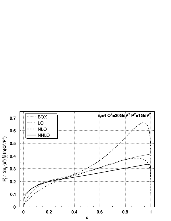
Figure 3: Virtual photon structure function $F_{2}^{\gamma}(x,Q^{2},P^{2})$ in units of $(3\alpha n_{f}\langle e^{4}\rangle/\pi)\ln(Q^{2}/P^{2})$ for $Q^{2}\!=\!30$ GeV² and $P^{2}\!=\!1$ GeV² with $n_{f}\!=\!4$ and the QCD scale parameter $\Lambda\!=\!0.2$ GeV. We plot the Box (tree) diagram contribution including non-leading corrections (short-dashed line), the QCD leading order (LO) (dash-dotted line), the next-to-leading order (NLO) (long-dashed line) and the next-to-next-to-leading order (NNLO) (solid line) results.

In Fig.3 we plot the virtual photon structure function $F_{2}^{\gamma}(x,Q^{2},P^{2})$ predicted by pQCD for the case of $n_{f}\!=\!4$, $Q^{2}\!=\!30$ GeV² and $P^{2}\!=\!1$ GeV² with the QCD scale parameter $\Lambda\!=\!0.2$ GeV. The vertical axis corresponds to

$$F_{2}^{\gamma}(x,Q^{2},P^{2})/\frac{3\alpha}{\pi}n_{f}\langle e^{4}\rangle\ln\frac{Q^{2}}{P^{2}}~{}.$$ (95)

Here we show four curves; the LO, NLO and NNLO QCD results and the Box (tree) diagram contribution including non-leading corrections. The box contribution is expressed by UW2

$$F_{2}^{\gamma({\rm Box})}(x,Q^{2},P^{2}) = \frac{3\alpha}{\pi}n_{f}\langle e^{4}\rangle\biggl{\{}x\Bigl{[}x^{2}+(1-x)^{2}\Bigr{]}\ln\frac{Q^{2}}{P^{2}}$$ (96)

$$\qquad\qquad-2x\Bigl{[}1-3x+3x^{2}+(1-2x+2x^{2})\ln x\Bigr{]}\biggr{\}}~{},$$

where power corrections $P^{2}/Q^{2}$ and quark mass effects are ignored. It is noted that, in these analyses, even for the LO and NLO QCD curves, we have used the QCD running coupling constant $\alpha_{s}(Q^{2})$ which is valid up to the three-loop level and is governed by the formula (90) and we have put $\Lambda\!=0.2$GeV.

The LO and NLO QCD results with the same values of $n_{f}$, $Q^{2}$ and $P^{2}$ as well as the Box contribution were already given in Fig.6 of Ref.UW2 . But in Ref.UW2 the formula for $\alpha_{s}(Q^{2})$ which is valid in the one-loop level was used to obtain the LO curve, while the two-loop level formula for $\alpha_{s}(Q^{2})$ was applied for the NLO graph, and the QCD scale parameter $\Lambda$ was set to be 0.1 GeV in both cases. The LO result in Fig.3 has a similar shape as the corresponding one in Ref.UW2 but is different in magnitude; the former is slightly larger than the latter for almost the whole $x$ region. This is due to the fact that the one-loop-level formula for $\alpha_{s}(Q^{2})$ was used for the LO curve in Ref.UW2 while we applied the three-loop-level formula even for the LO result. On the other hand, the NLO curve in Fig.3 is similar to the corresponding one in Ref.UW2 in shape and magnitude.

Now we observe in Fig.3 that there exist notable NNLO QCD corrections at larger $x$. The corrections are negative and the NNLO curve comes below the NLO one in the region $0.3\lesssim x<1$. This is expected from the $n\!=\!2$ moment analysis in Sec.IV. From Table 4 we see that the ratio of the NNLO to the sum of the LO and NLO contributions for the sum rule of $F_{2}^{\gamma}(x,Q^{2},P^{2})$ is  $-0.099$  for the case of $n_{f}\!=\!4$, $Q^{2}\!=\!30$ GeV² and $P^{2}\!=\!1$ GeV². At lower $x$ region, $0.05\lesssim x\lesssim 0.3$, the NNLO corrections to the NLO results are found to be negligibly small.

We have also studied the QCD corrections to $F_{2}^{\gamma}(x,Q^{2},P^{2})$ with different $Q^{2}$ and $P^{2}$ but with $n_{f}\!=\!4$.

Figure 4: Virtual photon structure function $F_{2}^{\gamma}(x,Q^{2},P^{2})$ for $Q^{2}\!=\!100$ GeV² and $P^{2}\!=\!1$ GeV² with $n_{f}\!=\!4$ and $\Lambda\!=\!0.2$ GeV.

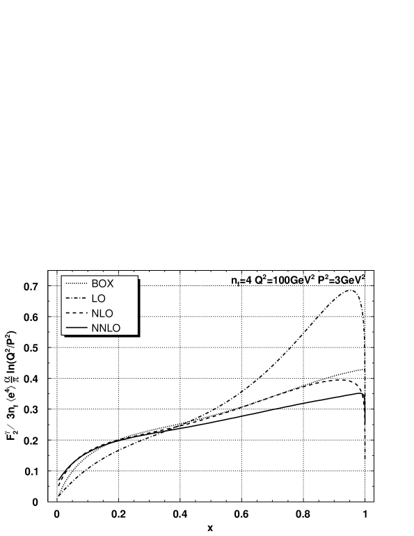
Figure 5: Virtual photon structure function $F_{2}^{\gamma}(x,Q^{2},P^{2})$ for $Q^{2}\!=\!100$ GeV² and $P^{2}\!=\!3$ GeV² with $n_{f}\!=\!4$ and $\Lambda\!=\!0.2$ GeV.

In Fig.4 we plot the case for $Q^{2}\!=\!100$ GeV² and $P^{2}\!=\!1$ GeV². Another case for $Q^{2}\!=\!100$ GeV² and $P^{2}\!=\!3$ GeV² is shown in Fig.5. We have not seen any sizable change for the normalized structure function (95) for these different values of $Q^{2}$ and $P^{2}$. In both cases the NNLO corrections reduce $F_{2}^{\gamma}(x,Q^{2},P^{2})$ at larger $x$. We have examined the $n_{f}=3$ case as well. It is observed that the normalized structure function (95) is insensitive to the number of active flavors.

Finally we should note that the spin-averaged structure function directly accessible in the experiment is not $F_{2}^{\gamma}$, but the so-called effective structure function $F_{\rm eff}^{\gamma}\simeq F_{2}^{\gamma}+(3/2)F_{L}^{\gamma}$ as discussed in ref. Krawczyk ; GRStratmann ; GRSchienbein

VI Longitudinal structure function $F_{L}^{\gamma}(x,Q^{2},P^{2})$

We have considered the structure function $F_{2}^{\gamma}$ so far. Regarding another structure function $F_{L}^{\gamma}$, its LO contribution, which is of order $\alpha$, was calculated in QCD for the real photon ($P^{2}\!=\!0$) target in Refs.Witten ; BB . The analysis was extended to the case of the virtual photon ($\Lambda^{2}\ll P^{2}\ll Q^{2}$) target UW2 . We will now derive a formula for the moment sum rule of $F_{L}^{\gamma}(x,Q^{2},P^{2})$ up to the NLO (${\cal O}(\alpha\alpha_{s}$)) corrections. Comparing Eq.(12b) with (12a) and examining the form of (15), we see that the formula for $F_{L}^{\gamma}(x,Q^{2},P^{2})$ is obtained from (22) only by replacing $\bm{C}_{2,n}(1,{\bar{g}}(Q^{2}))$ and $C_{2,n}^{\gamma}(1,{\bar{g}}(Q^{2}),\alpha)$ with $\bm{C}_{L,n}(1,{\bar{g}}(Q^{2}))$ and $C_{L,n}^{\gamma}(1,{\bar{g}}(Q^{2}),\alpha)$, respectively. An expansion is made for $\bm{C}_{L,n}(1,{\bar{g}}(Q^{2}))$ and $C_{L,n}^{\gamma}(1,{\bar{g}}(Q^{2}),\alpha)$ up to the two-loop level as

$${\bm{C}}_{L,n}(1,{\bar{g}}(Q^{2})) = {\bm{C}}_{L,n}^{(0)}+\frac{{\bar{g}}^{2}(Q^{2})}{16\pi^{2}}{\bm{C}}_{L,n}^{(1)}+\frac{{\bar{g}}^{4}(Q^{2})}{(16\pi^{2})^{2}}{\bm{C}}_{L,n}^{(2)}+\cdots~{},$$ (97)

$$C_{L,n}^{\gamma}(1,{\bar{g}}(Q^{2}),\alpha) = \frac{e^{2}}{16\pi^{2}}C_{L,n}^{\gamma(1)}+\frac{e^{2}{\bar{g}}^{2}(Q^{2})}{(16\pi^{2})^{2}}C_{L,n}^{\gamma(2)}+\cdots~{}.$$ (98)

Here we note that there is no contribution of the tree diagrams to the longitudinal coefficient functions and thus we have ${\bm{C}}_{L,n}^{(0)}={\bm{0}}$.

The moments of $F_{L}^{\gamma}(x,Q^{2},P^{2})$ are then given as follows (see Eqs.(33)-(41) for comparison):

$$\int_{0}^{1}dxx^{n-2}F_{L}^{\gamma}(x,Q^{2},P^{2})$$ (99)

$$= \frac{\alpha}{4\pi}\frac{1}{2\beta_{0}}\Biggl{\{}\sum_{i}{\cal B}_{(L),i}^{n}\left[1-\left(\frac{\alpha_{s}(Q^{2})}{\alpha_{s}(P^{2})}\right)^{d_{i}^{n}+1}\right]+{\cal C}_{(L)}^{n}$$

$$\qquad+\frac{\alpha_{s}(Q^{2})}{4\pi}\biggl{(}\sum_{i}{\cal E}_{(L),i}^{n}\left[1-\left(\frac{\alpha_{s}(Q^{2})}{\alpha_{s}(P^{2})}\right)^{d_{i}^{n}}\right]+\sum_{i}{\cal F}_{(L),i}^{n}\left[1-\left(\frac{\alpha_{s}(Q^{2})}{\alpha_{s}(P^{2})}\right)^{d_{i}^{n}+1}\right]$$

$$\hskip 99.58464pt+{\cal G}_{(L)}^{n}\biggr{)}+{\cal O}(\alpha_{s}^{2})\Biggr{\}}~{},\hskip 56.9055pt{\rm with}\quad i=+,-,NS~{},$$

where the coefficients ${\cal B}^{n}_{(L),i}$, ${\cal C}^{n}_{(L)}$, ${\cal E}^{n}_{(L),i}$, ${\cal F}^{n}_{(L),i}$ and ${\cal G}^{n}_{(L)}$ are

$${\cal B}^{n}_{(L),i} = \bm{K}_{n}^{(0)}P^{n}_{i}{\bm{C}}_{L,n}^{(1)}\frac{1}{1+d_{i}^{n}}~{},$$ (100)

$${\cal C}^{n}_{(L)} = 2\beta_{0}C_{L,n}^{\gamma(1)}~{},$$ (101)

$${\cal E}^{n}_{(L),i} = -\bm{K}_{n}^{(0)}P^{n}_{i}{\bm{C}}_{L,n}^{(1)}\frac{\beta_{1}}{\beta_{0}}\frac{1-d_{i}^{n}}{d_{i}^{n}}-\bm{K}_{n}^{(0)}\sum_{j}\frac{P^{n}_{j}\hat{\gamma}_{n}^{(1)}P^{n}_{i}}{\lambda^{n}_{j}-\lambda^{n}_{i}+2\beta_{0}}{\bm{C}}_{L,n}^{(1)}\frac{1}{d_{i}^{n}}$$ (102)

$$+\bm{K}_{n}^{(1)}P^{n}_{i}{\bm{C}}_{L,n}^{(1)}\frac{1}{d_{i}^{n}}-2\beta_{0}{\widetilde{\bm{A}}}_{n}^{(1)}P^{n}_{i}{\bm{C}}_{L,n}^{(1)}~{},$$

$${\cal F}^{n}_{(L),i} = \bm{K}_{n}^{(0)}P^{n}_{i}{\bm{C}}_{L,n}^{(2)}\frac{1}{1+d_{i}^{n}}-\bm{K}_{n}^{(0)}P^{n}_{i}{\bm{C}}_{L,n}^{(1)}\frac{\beta_{1}}{\beta_{0}}\frac{d_{i}^{n}}{1+d_{i}^{n}}$$ (103)

$$+\bm{K}_{n}^{(0)}\sum_{j}\frac{P^{n}_{i}\hat{\gamma}_{n}^{(1)}P^{n}_{j}}{\lambda^{n}_{i}-\lambda^{n}_{j}+2\beta_{0}}{\bm{C}}_{L,n}^{(1)}\frac{1}{1+d_{i}^{n}}~{},$$

$${\cal G}^{n}_{(L)} = 2\beta_{0}(C_{L,n}^{\gamma(2)}+{\widetilde{\bm{A}}}_{n}^{(1)}\cdot{\bm{C}}_{L,n}^{(1)})~{},$$ (104)

with $i,j=+,-,NS$. The coefficients ${\cal B}^{n}_{(L),i}$ and ${\cal C}^{n}_{(L)}$ represent the LO terms Witten ; BB ; UW2 , while the terms with ${\cal E}^{n}_{(L),i}$, ${\cal F}^{n}_{(L),i}$ and ${\cal G}^{n}_{(L)}$ are the NLO ($\alpha\alpha_{s}$) corrections and new. It is noted that, among these coefficients, ${\cal E}^{n}_{(L),-}$ becomes singular at $n\!=\!2$ since it has terms with the factor $\frac{1}{d_{-}^{n}}$ and $d_{-}^{n}$ vanishes as $n\!\rightarrow\!2$. But again, as in the case of the moments of $F_{2}^{\gamma}(x,Q^{2},P^{2})$, this coefficient is multiplied by a factor $\Bigl{[}1-\Bigl{(}\alpha_{s}(Q^{2})/\alpha_{s}(P^{2})\Bigr{)}^{d_{-}^{n}}\Bigr{]}$, and thus the product remain finite at $n\!=\!2$.

The one-loop longitudinal coefficient functions were well known ZWT ; HL ; BBDM . They are written in the form as

$$C_{L,n}^{\psi(1)}=\delta_{\psi}B^{n}_{\psi,L},\quad C_{L,n}^{G(1)}=\delta_{\psi}B^{n}_{G,L}~{},\quad C_{L,n}^{NS(1)}=\delta_{NS}B^{n}_{NS,L}~{},\quad C_{L,n}^{\gamma(1)}=\delta_{\gamma}B^{n}_{\gamma,L}~{},$$ (105)

where $B^{n}_{\psi,L}=B^{n}_{NS,L}$, $B^{n}_{G,L}$ and $B^{n}_{\gamma,L}$ are given, for example, in Eqs.(6.2) - (6.4) of Ref.BB . The two-loop longitudinal coefficient functions corresponding to the hadronic operators were calculated in the $\overline{\rm MS}$ scheme in Ref.vNZ ; ZvN1 . The results in Mellin space as functions of $n$ are found, for example, in Ref. MochVermaseren :

$$C_{L,n}^{\psi(2)} = \delta_{\psi}~{}\Bigl{\{}c_{L,q}^{(2),{\rm ns}}(n)+c_{L,q}^{(2),{\rm ps}}(n)\Bigr{\}},$$ (106)

$$C_{L,n}^{G(2)} = \delta_{\psi}~{}c_{L,g}^{(2)}(n),$$ (107)

$$\quad C_{L,n}^{NS(2)} = \delta_{NS}~{}c_{L,q}^{(2),{\rm ns}}(n)~{}.~{}$$ (108)

where $c_{L,q}^{(2),{\rm ns}}(n)$, $c_{L,q}^{(2),{\rm ps}}(n)$ and $c_{L,g}^{(2)}(n)$ are given in Eqs.(203), (204), and (205) in Appendix B of Ref.MochVermaseren , respectively, with $N$ being replaced by $n$. The two-loop photon longitudinal coefficient function $C_{L,n}^{\gamma(2)}$ is expressed as

$$C_{L,n}^{\gamma(2)}=\delta_{\gamma}c_{L,\gamma}^{(2)}(n)~{},$$ (109)

and $c_{L,\gamma}^{(2)}(n)$ is obtained from $c_{L,g}^{(2)}(n)$ in (107) by replacing $C_{A}\rightarrow 0$ and $\frac{n_{f}}{2}\rightarrow 1$.

Inverting the moments (99), we plot in Fig.6 the longitudinal virtual photon structure function $F_{L}^{\gamma}(x,Q^{2},P^{2})$ predicted by pQCD for the case of $n_{f}\!=\!4$, $Q^{2}\!=\!30$ GeV² and $P^{2}\!=\!1$ GeV² with the QCD scale parameter $\Lambda\!=\!0.2$ GeV. The vertical axis is in units of $F_{L}^{\gamma}(x,Q^{2},P^{2})/\frac{3\alpha}{\pi}n_{f}\langle e^{4}\rangle$. Here we show three curves; the LO and NLO QCD results and the Box (tree) diagram contribution, which is expressed by

$$F_{L}^{\gamma({\rm Box})}(x,Q^{2},P^{2})=\frac{3\alpha}{\pi}n_{f}\langle e^{4}\rangle\Bigl{\{}4x^{2}(1-x)\Bigr{\}}~{}.$$ (110)

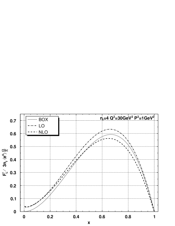
Figure 6: Longitudinal photon structure function $F_{L}^{\gamma}(x,Q^{2},P^{2})$ in units of $(3\alpha n_{f}\langle e^{4}\rangle/\pi)$ for $Q^{2}\!=\!30$ GeV² and $P^{2}\!=\!1$ GeV² with $n_{f}\!=\!4$ and the QCD scale parameter $\Lambda\!=\!0.2$ GeV. We plot the Box (tree) diagram contribution (short-dashed line), the QCD leading order (LO) (dash-dotted line) and the next-to-leading order (NLO) (long-dashed line) results.

The LO result in Fig.6 is consistent with the corresponding one in Fig.5 of Ref.UW2 , although the formulae used for $\alpha_{s}(Q^{2})$ differ in detail. We see from Fig.6 that the NLO QCD corrections are negative and the NLO curve comes below the LO one in the region $0.2\lesssim x<1$.

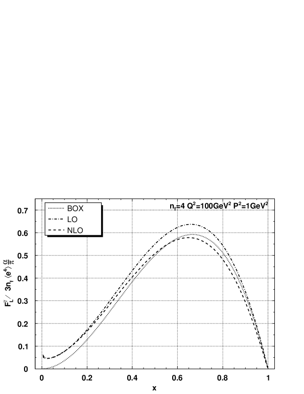
Figure 7: Longitudinal photon structure function $F_{L}^{\gamma}(x,Q^{2},P^{2})$ for $Q^{2}\!=\!100$ GeV² and $P^{2}\!=\!1$ GeV² with $n_{f}\!=\!4$ and $\Lambda\!=\!0.2$ GeV.

The QCD corrections to $F_{L}^{\gamma}(x,Q^{2},P^{2})$ for different values of $Q^{2}$, $P^{2}$ and $n_{f}$ are also studied. The case for $Q^{2}\!=\!100$ GeV² and $P^{2}\!=\!1$ GeV² with $n_{f}\!=\!4$ is shown in Fig.7. The LO curve has hardly changed from the one for $Q^{2}\!=\!30$ GeV² and $P^{2}\!=\!1$ GeV². The NLO corrections get smaller. The LO and NLO QCD curves for $Q^{2}\!=\!100$ GeV² and $P^{2}\!=\!3$ GeV² with $n_{f}\!=\!4$ appear to be almost the same as those in the case of $Q^{2}\!=\!30$ GeV² and $P^{2}\!=\!1$. The cases for $n_{f}\!=\!3$ are examined as well and we find that the normalized function $F_{L}^{\gamma}(x,Q^{2},P^{2})/\frac{3\alpha}{\pi}n_{f}\langle e^{4}\rangle$ is insensitive to the number of active flavors.

VII Conclusions

We have investigated the unpolarized virtual photon structure functions $F_{2}^{\gamma}(x,Q^{2},P^{2})$ and $F_{L}^{\gamma}(x,Q^{2},P^{2})$ for the kinematical region $\Lambda^{2}\ll P^{2}\ll Q^{2}$ in QCD. In the framework of the OPE supplemented by the RG method, we gave the definite predictions for the moments of $F_{2}^{\gamma}(x,Q^{2},P^{2})$ up to the NNLO (the order $\alpha\alpha_{s}$) and for the moments of $F_{L}^{\gamma}(x,Q^{2},P^{2})$ up to the NLO (the order $\alpha\alpha_{s}$). In the course of our evaluation, we utilized the recently calculated results of the three-loop anomalous dimensions for the quark and gluon operators. Also we derived the photon matrix elements of hadronic operators up to the two-loop level.

The sum rule of $F_{2}^{\gamma}(x,Q^{2},P^{2})$, i.e., the second moment, was numerically examined. The NNLO corrections are found to be $7\%\sim 10\%$ of the sum of the LO and NLO contributions, when $P^{2}\!=\!1{\rm GeV}^{2}$ and $Q^{2}\!=\!30\sim 100{\rm GeV}^{2}$ or $P^{2}\!=\!3{\rm GeV}^{2}$ and $Q^{2}\!=\!100{\rm GeV}^{2}$, and $n_{f}$ is three or four.

The inverse Mellin transform of the moments was performed to express the structure functions $F_{2}^{\gamma}(x,Q^{2},P^{2})$ and $F_{L}^{\gamma}(x,Q^{2},P^{2})$ as functions of $x$. We found that there exist sizable NNLO contributions for $F_{2}^{\gamma}$ at larger $x$. The corrections are negative and the NNLO curve comes below the NLO one in the region $0.3\lesssim x<1$. At lower $x$ region, $0.05\lesssim x\lesssim 0.3$, the NNLO corrections to the NLO results are found to be negligibly small. Concerning $F_{L}^{\gamma}$, the NLO corrections reduce the magnitude in the region $0.2\lesssim x<1$.

The comparison of the present NNLO theoretical prediction for the virtual photon structure functions with the existing experimental data will be discussed elsewhere.

Appendix A Evaluation of $M_{n}(Q^{2}/P^{2},{\bar{g}}(P^{2}))$ and $\bm{X}_{n}(Q^{2}/P^{2},{\bar{g}}(P^{2}),\alpha)$

In order to evaluate the integrals for $M_{n}(Q^{2}/P^{2},{\bar{g}}(P^{2}))$ given in (26), we employ the same method that was used by Bardeen and Buras in Ref.BB and make a full use of the projection operators obtained from the one-loop anomalous dimension matrix ${\widehat{\gamma}}^{0}_{n}$:

$${\widehat{\gamma}}^{(0)}_{n}=\sum_{i=+,-,NS}\lambda^{n}_{i}~{}P^{n}_{i}~{},$$ (111)

where $\lambda^{n}_{i}~{}(i=+,-,NS)$ are eigenvalues of ${\widehat{\gamma}}^{0}_{n}$ and are expressed as

$$\lambda^{n}_{\pm} = \frac{1}{2}\Bigl{\{}\gamma^{(0),n}_{\psi\psi}+\gamma^{(0),n}_{GG}\pm\Bigl{[}(\gamma^{(0),n}_{\psi\psi}-\gamma^{(0),n}_{GG})^{2}+4\gamma^{(0),n}_{\psi G}\gamma^{(0),n}_{G\psi}\Bigr{]}^{1/2}\Bigr{\}}~{},$$ (112)

$$\lambda^{n}_{NS} = \gamma^{(0),n}_{NS}~{},$$ (113)

and $P^{n}_{i}$ are the corresponding projection operators,

$$P^{n}_{\pm} = \frac{1}{\lambda^{n}_{\pm}-\lambda^{n}_{\mp}}\begin{pmatrix}\gamma^{(0),n}_{\psi\psi}-\lambda^{n}_{\mp}&\gamma^{(0),n}_{G\psi}&0\\ \gamma^{(0),n}_{\psi G}&\gamma^{(0),n}_{GG}-\lambda^{n}_{\mp}&0\\ 0&0&0\end{pmatrix}~{},$$ (114)

$$P^{n}_{NS} = \begin{pmatrix}0&0&0\\ 0&0&0\\ 0&0&1\end{pmatrix}~{}.$$ (115)

With an expansion of $\beta(g)$ up to the three-loop level in (28), we get its inverse as follows:

$$\frac{1}{\beta(g)}=-\frac{16\pi^{2}}{\beta_{0}}\frac{1}{g^{3}}\left\{1-\frac{g^{2}}{16\pi^{2}}\frac{\beta_{1}}{\beta_{0}}+\frac{g^{4}}{(16\pi^{2})^{2}}\left(\frac{\beta_{1}^{2}}{\beta_{0}^{2}}-\frac{\beta_{2}}{\beta_{0}}\right)+\cdots\right\}~{}.$$ (116)

Then using (111) and (116), we perform integration in (26).

The result is

$$M_{n}(Q^{2}/P^{2},{\bar{g}}(P^{2}))$$ (117)

$$= \sum_{i}P_{i}^{n}\left(\frac{{\bar{g}}_{2}^{2}}{{\bar{g}}_{1}^{2}}\right)^{d_{i}^{n}}+\frac{1}{16\pi^{2}}\sum_{i}P_{i}^{n}\left(\frac{{\bar{g}}_{2}^{2}}{{\bar{g}}_{1}^{2}}\right)^{d_{i}^{n}}d_{i}^{n}~{}\frac{\beta_{1}}{\beta_{0}}({\bar{g}}_{1}^{2}-{\bar{g}}_{2}^{2})$$

$$- \frac{1}{16\pi^{2}}\sum_{i,j}P_{i}^{n}{\hat{\bm{\gamma}}}_{n}^{(1)}P_{j}^{n}\frac{1}{\lambda_{i}^{n}-\lambda_{j}^{n}+2\beta_{0}}\biggl{[}{\bar{g}}_{1}^{2}\Bigl{(}\frac{{\bar{g}}_{2}^{2}}{{\bar{g}}_{1}^{2}}\Bigr{)}^{d_{j}^{n}}-{\bar{g}}_{2}^{2}\Bigl{(}\frac{{\bar{g}}_{2}^{2}}{{\bar{g}}_{1}^{2}}\Bigr{)}^{d_{i}^{n}}\biggr{]}$$

$$+ \frac{1}{(16\pi^{2})^{2}}\sum_{i}P_{i}^{n}\left(\frac{{\bar{g}}_{2}^{2}}{{\bar{g}}_{1}^{2}}\right)^{d_{i}^{n}}\frac{1}{2}\biggl{\{}-d_{i}^{n}\Bigl{[}\frac{\beta_{1}^{2}}{\beta_{0}^{2}}-\frac{\beta_{2}}{\beta_{0}}\Bigr{]}({\bar{g}}_{1}^{4}-{\bar{g}}_{2}^{4})+\Bigl{(}d_{i}^{n}~{}\frac{\beta_{1}}{\beta_{0}}\Bigr{)}^{2}({\bar{g}}_{1}^{2}-{\bar{g}}_{2}^{2})^{2}\biggr{\}}$$

$$- \frac{1}{(16\pi^{2})^{2}}\sum_{i,j}P_{i}^{n}{\hat{\bm{\gamma}}}_{n}^{(1)}P_{j}^{n}\frac{1}{\lambda_{i}^{n}-\lambda_{j}^{n}+2\beta_{0}}~{}\frac{\beta_{1}}{\beta_{0}}\Bigl{(}d_{i}^{n}{\bar{g}}_{1}^{2}-d_{j}^{n}{\bar{g}}_{2}^{2}\Bigr{)}\biggl{[}{\bar{g}}_{1}^{2}\Bigl{(}\frac{{\bar{g}}_{2}^{2}}{{\bar{g}}_{1}^{2}}\Bigr{)}^{d_{j}^{n}}-{\bar{g}}_{2}^{2}\Bigl{(}\frac{{\bar{g}}_{2}^{2}}{{\bar{g}}_{1}^{2}}\Bigr{)}^{d_{i}^{n}}\biggr{]}$$

$$+ \frac{1}{(16\pi^{2})^{2}}\sum_{i,j}P_{i}^{n}{\hat{\bm{\gamma}}}_{n}^{(1)}P_{j}^{n}\frac{\Bigl{(}1+d_{i}^{n}-d_{j}^{n}\Bigr{)}}{\lambda_{i}^{n}-\lambda_{j}^{n}+4\beta_{0}}~{}\frac{\beta_{1}}{\beta_{0}}\biggl{[}({\bar{g}}_{1}^{2})^{2}\Bigl{(}\frac{{\bar{g}}_{2}^{2}}{{\bar{g}}_{1}^{2}}\Bigr{)}^{d_{j}^{n}}-({\bar{g}}_{2}^{2})^{2}\Bigl{(}\frac{{\bar{g}}_{2}^{2}}{{\bar{g}}_{1}^{2}}\Bigr{)}^{d_{i}^{n}}\biggr{]}$$

$$- \frac{1}{(16\pi^{2})^{2}}\sum_{i,j}~{}\frac{P^{n}_{i}{\hat{\bm{\gamma}}}_{n}^{(2)}P^{n}_{j}}{\lambda^{n}_{i}-\lambda^{n}_{j}+4\beta_{0}}\biggl{[}({\bar{g}}_{1}^{2})^{2}\Bigl{(}\frac{{\bar{g}}_{2}^{2}}{{\bar{g}}_{1}^{2}}\Bigr{)}^{d_{j}^{n}}-({\bar{g}}_{2}^{2})^{2}\Bigl{(}\frac{{\bar{g}}_{2}^{2}}{{\bar{g}}_{1}^{2}}\Bigr{)}^{d_{i}^{n}}\biggr{]}$$

$$+ \frac{1}{(16\pi^{2})^{2}}\sum_{i,j,k}P^{n}_{i}{\hat{\bm{\gamma}}}_{n}^{(1)}P^{n}_{j}{\hat{\bm{\gamma}}}_{n}^{(1)}P^{n}_{k}\frac{1}{(\lambda^{n}_{j}-\lambda^{n}_{k}+2\beta_{0})}$$

$$\qquad\qquad\times\Biggl{[}\frac{1}{\lambda^{n}_{i}-\lambda^{n}_{k}+4\beta_{0}}\biggl{\{}({\bar{g}}_{1}^{2})^{2}\Bigl{(}\frac{{\bar{g}}_{2}^{2}}{{\bar{g}}_{1}^{2}}\Bigr{)}^{d_{k}^{n}}-({\bar{g}}_{2}^{2})^{2}\Bigl{(}\frac{{\bar{g}}_{2}^{2}}{{\bar{g}}_{1}^{2}}\Bigr{)}^{d_{i}^{n}}\biggr{\}}$$

$$\qquad\qquad\qquad\qquad-\frac{1}{\lambda^{n}_{i}-\lambda^{n}_{j}+2\beta_{0}}\biggl{\{}{\bar{g}}_{1}^{2}~{}{\bar{g}}_{2}^{2}~{}\Bigl{(}\frac{{\bar{g}}_{2}^{2}}{{\bar{g}}_{1}^{2}}\Bigr{)}^{d_{j}^{n}}-({\bar{g}}_{2}^{2})^{2}\Bigl{(}\frac{{\bar{g}}_{2}^{2}}{{\bar{g}}_{1}^{2}}\Bigr{)}^{d_{i}^{n}}\biggr{\}}\Biggr{]}~{},$$

where ${\bar{g}}_{1}^{2}={\bar{g}}^{2}(P^{2})$ and ${\bar{g}}_{2}^{2}={\bar{g}}^{2}(Q^{2})$. The first term is the leading, and the second and third terms are the next-to-leading terms. The rest are the next-to-next-to-leading terms.

Once we get the above expression for $M_{n}(Q^{2}/P^{2},{\bar{g}}(P^{2}))$ expanded up to the NNLO, we use an expansion of ${\bm{K}}_{n}(g,\alpha)$ in (29) up to the three-loop level and can evaluate $\bm{X}_{n}(Q^{2}/P^{2},{\bar{g}}(P^{2}),\alpha)$ in (21) up to the NNLO. The result is

$$\bm{X}_{n}(Q^{2}/P^{2},{\bar{g}}(P^{2}),\alpha)$$

$$= \frac{e^{2}}{2\beta_{0}}\frac{1}{{\bar{g}}_{2}^{2}}\bm{K}_{n}^{(0)}\sum_{i}P_{i}^{n}\frac{1}{d_{i}^{n}+1}\biggl{[}1-\biggl{(}\frac{{\bar{g}}_{2}^{2}}{{\bar{g}}_{1}^{2}}\biggr{)}^{d_{i}^{n}+1}\biggr{]}$$

$$+ \frac{e^{2}}{2\beta_{0}}\frac{1}{16\pi^{2}}\bm{K}_{n}^{(0)}\frac{\beta_{1}}{\beta_{0}}\sum_{i}P_{i}^{n}\biggl{\{}-\frac{d_{i}^{n}}{d_{i}^{n}+1}\biggl{[}1-\biggl{(}\frac{{\bar{g}}_{2}^{2}}{{\bar{g}}_{1}^{2}}\biggr{)}^{d_{i}^{n}+1}\biggr{]}+\frac{d_{i}^{n}-1}{d_{i}^{n}}\biggl{[}1-\biggl{(}\frac{{\bar{g}}_{2}^{2}}{{\bar{g}}_{1}^{2}}\biggr{)}^{d_{i}^{n}}\biggr{]}\biggr{\}}$$

$$+ \frac{e^{2}}{2\beta_{0}}\frac{1}{16\pi^{2}}\bm{K}_{n}^{(0)}\sum_{i}\biggl{\{}\sum_{j}\frac{P_{i}^{n}{\hat{\bm{\gamma}}}_{n}^{(1)}P_{j}^{n}}{\lambda_{i}^{n}-\lambda_{j}^{n}+2\beta_{0}}\frac{1}{d_{i}^{n}+1}\biggl{[}1-\biggl{(}\frac{{\bar{g}}_{2}^{2}}{{\bar{g}}_{1}^{2}}\biggr{)}^{d_{i}^{n}+1}\biggr{]}$$

$$\hskip 99.58464pt-\sum_{j}\frac{P_{j}^{n}{\hat{\bm{\gamma}}}_{n}^{(1)}P_{i}^{n}}{\lambda_{j}^{n}-\lambda_{i}^{n}+2\beta_{0}}\frac{1}{d_{i}^{n}}\biggl{[}1-\biggl{(}\frac{{\bar{g}}_{2}^{2}}{{\bar{g}}_{1}^{2}}\biggr{)}^{d_{i}^{n}}\biggr{]}\biggr{\}}$$

$$+ \frac{e^{2}}{2\beta_{0}}\frac{1}{16\pi^{2}}~{}\bm{K}_{n}^{(1)}\sum_{i}P_{i}^{n}\frac{1}{d_{i}^{n}}\biggl{[}1-\biggl{(}\frac{{\bar{g}}_{2}^{2}}{{\bar{g}}_{1}^{2}}\biggr{)}^{d_{i}^{n}}\biggr{]}$$

$$+ \frac{e^{2}}{2\beta_{0}}\frac{{\bar{g}}_{2}^{2}}{(16\pi^{2})^{2}}\bm{K}_{n}^{(0)}\sum_{i}P_{i}^{n}~{}\Biggl{\{}\frac{d_{i}^{n}}{2}\biggl{(}\frac{\beta_{1}^{2}}{\beta_{0}^{2}}-\frac{\beta_{2}}{\beta_{0}}\frac{1}{d_{i}^{n}+1}\biggr{)}\biggl{[}1-\biggl{(}\frac{{\bar{g}}_{2}^{2}}{{\bar{g}}_{1}^{2}}\biggr{)}^{d_{i}^{n}+1}\biggr{]}$$

$$\ +\frac{\beta_{1}^{2}}{\beta_{0}^{2}}~{}(1-d_{i}^{n})~{}\biggl{[}1-\biggl{(}\frac{{\bar{g}}_{2}^{2}}{{\bar{g}}_{1}^{2}}\biggr{)}^{d_{i}^{n}}\biggr{]}+\Bigl{(}\frac{d_{i}^{n}}{2}-1\Bigr{)}\biggl{(}\frac{\beta_{1}^{2}}{\beta_{0}^{2}}+\frac{\beta_{2}}{\beta_{0}}\frac{1}{d_{i}^{n}-1}\biggr{)}\biggl{[}1-\biggl{(}\frac{{\bar{g}}_{2}^{2}}{{\bar{g}}_{1}^{2}}\biggr{)}^{d_{i}^{n}-1}\biggr{]}\Biggr{\}}$$

$$+ \frac{e^{2}}{2\beta_{0}}\frac{{\bar{g}}_{2}^{2}}{(16\pi^{2})^{2}}\bm{K}_{n}^{(0)}\frac{\beta_{1}}{\beta_{0}}\sum_{i}$$

$$\quad\times\Biggl{\{}\biggl{(}-\sum_{j}\frac{P_{i}^{n}{\hat{\bm{\gamma}}}_{n}^{(1)}P_{j}^{n}}{\lambda_{i}^{n}-\lambda_{j}^{n}+2\beta_{0}}\frac{d_{j}^{n}}{d_{i}^{n}+1}-\sum_{j}\frac{P_{i}^{n}{\hat{\bm{\gamma}}}_{n}^{(1)}P_{j}^{n}}{\lambda_{i}^{n}-\lambda_{j}^{n}+4\beta_{0}}\frac{1+d_{i}^{n}-d_{j}^{n}}{d_{i}^{n}+1}\biggr{)}$$

$$\hskip 241.84842pt\times\biggl{[}1-\biggl{(}\frac{{\bar{g}}_{2}^{2}}{{\bar{g}}_{1}^{2}}\biggr{)}^{d_{i}^{n}+1}\biggr{]}$$

$$\qquad+\biggl{(}\sum_{j}\frac{P_{i}^{n}{\hat{\bm{\gamma}}}_{n}^{(1)}P_{j}^{n}}{\lambda_{i}^{n}-\lambda_{j}^{n}+2\beta_{0}}\Bigl{(}1-\frac{1}{d_{i}^{n}}\Bigr{)}+\sum_{j}\frac{P_{j}^{n}{\hat{\bm{\gamma}}}_{n}^{(1)}P_{i}^{n}}{\lambda_{j}^{n}-\lambda_{i}^{n}+2\beta_{0}}\biggr{)}\biggl{[}1-\biggl{(}\frac{{\bar{g}}_{2}^{2}}{{\bar{g}}_{1}^{2}}\biggr{)}^{d_{i}^{n}}\biggr{]}$$

$$\qquad+\biggl{(}\sum_{j}\frac{P_{j}^{n}{\hat{\bm{\gamma}}}_{n}^{(1)}P_{i}^{n}}{\lambda_{j}^{n}-\lambda_{i}^{n}+2\beta_{0}}\frac{1-d_{j}^{n}}{d_{i}^{n}-1}+\sum_{j}\frac{P_{j}^{n}{\hat{\bm{\gamma}}}_{n}^{(1)}P_{i}^{n}}{\lambda_{j}^{n}-\lambda_{i}^{n}+4\beta_{0}}\frac{1+d_{j}^{n}-d_{i}^{n}}{d_{i}^{n}-1}\biggr{)}$$

$$\hskip 241.84842pt\times\biggl{[}1-\biggl{(}\frac{{\bar{g}}_{2}^{2}}{{\bar{g}}_{1}^{2}}\biggr{)}^{d_{i}^{n}-1}\biggr{]}\Biggr{\}}$$

$$+ \frac{e^{2}}{2\beta_{0}}\frac{{\bar{g}}_{2}^{2}}{(16\pi^{2})^{2}}\bm{K}_{n}^{(0)}\sum_{i}\biggl{\{}\sum_{j}\frac{P^{n}_{i}{\hat{\bm{\gamma}}}_{n}^{(2)}P^{n}_{j}}{\lambda^{n}_{i}-\lambda^{n}_{j}+4\beta_{0}}\frac{1}{d_{i}^{n}+1}\biggl{[}1-\biggl{(}\frac{{\bar{g}}_{2}^{2}}{{\bar{g}}_{1}^{2}}\biggr{)}^{d_{i}^{n}+1}\biggr{]}$$

$$\hskip 99.58464pt-\sum_{j}\frac{P^{n}_{j}{\hat{\bm{\gamma}}}_{n}^{(2)}P^{n}_{i}}{\lambda^{n}_{j}-\lambda^{n}_{i}+4\beta_{0}}\frac{1}{d_{i}^{n}-1}\biggl{[}1-\biggl{(}\frac{{\bar{g}}_{2}^{2}}{{\bar{g}}_{1}^{2}}\biggr{)}^{d_{i}^{n}-1}\biggr{]}\biggr{\}}$$

$$+\frac{e^{2}}{2\beta_{0}}\frac{{\bar{g}}_{2}^{2}}{(16\pi^{2})^{2}}\bm{K}_{n}^{(0)}\sum_{i}$$

$$\times\Biggl{\{}\sum_{j,k}\frac{P^{n}_{i}{\hat{\bm{\gamma}}}_{n}^{(1)}P^{n}_{j}{\hat{\bm{\gamma}}}_{n}^{(1)}P^{n}_{k}}{\lambda^{n}_{j}-\lambda^{n}_{k}+2\beta_{0}}\biggl{(}\frac{1}{\lambda^{n}_{i}-\lambda^{n}_{j}+2\beta_{0}}-\frac{1}{\lambda^{n}_{i}-\lambda^{n}_{k}+4\beta_{0}}\biggr{)}$$

$$\hskip 142.26378pt\times\frac{1}{d_{i}^{n}+1}\biggl{[}1-\biggl{(}\frac{{\bar{g}}_{2}^{2}}{{\bar{g}}_{1}^{2}}\biggr{)}^{d_{i}^{n}+1}\biggr{]}$$

$$-\sum_{j,k}\frac{P^{n}_{j}{\hat{\bm{\gamma}}}_{n}^{(1)}P^{n}_{i}{\hat{\bm{\gamma}}}_{n}^{(1)}P^{n}_{k}}{\lambda^{n}_{i}-\lambda^{n}_{k}+2\beta_{0}}\frac{1}{\lambda^{n}_{j}-\lambda^{n}_{i}+2\beta_{0}}~{}\frac{1}{d_{i}^{n}}\biggl{[}1-\biggl{(}\frac{{\bar{g}}_{2}^{2}}{{\bar{g}}_{1}^{2}}\biggr{)}^{d_{i}^{n}}\biggr{]}$$

$$+\sum_{j,k}\frac{P^{n}_{k}{\hat{\bm{\gamma}}}_{n}^{(1)}P^{n}_{j}{\hat{\bm{\gamma}}}_{n}^{(1)}P^{n}_{i}}{\lambda^{n}_{j}-\lambda^{n}_{i}+2\beta_{0}}\frac{1}{\lambda^{n}_{k}-\lambda^{n}_{i}+4\beta_{0}}~{}\frac{1}{d_{i}^{n}-1}\biggl{[}1-\biggl{(}\frac{{\bar{g}}_{2}^{2}}{{\bar{g}}_{1}^{2}}\biggr{)}^{d_{i}^{n}-1}\biggr{]}\Biggr{\}}$$

$$+\frac{e^{2}}{2\beta_{0}}\frac{{\bar{g}}^{2}_{2}}{(16\pi^{2})^{2}}\bm{K}_{n}^{(1)}\frac{\beta_{1}}{\beta_{0}}\sum_{i}P_{i}^{n}\biggl{\{}-\biggl{[}1-\biggl{(}\frac{{\bar{g}}_{2}^{2}}{{\bar{g}}_{1}^{2}}\biggr{)}^{d_{i}^{n}}\biggr{]}+\biggl{[}1-\biggl{(}\frac{{\bar{g}}_{2}^{2}}{{\bar{g}}_{1}^{2}}\biggr{)}^{d_{i}^{n}-1}\biggr{]}\biggr{\}}$$

$$+\frac{e^{2}}{2\beta_{0}}\frac{{\bar{g}}^{2}_{2}}{(16\pi^{2})^{2}}\bm{K}_{n}^{(1)}\sum_{i}\biggl{\{}\sum_{j}\frac{P_{i}^{n}{\hat{\bm{\gamma}}}_{n}^{(1)}P_{j}^{n}}{\lambda_{i}^{n}-\lambda_{j}^{n}+2\beta_{0}}~{}\frac{1}{d_{i}^{n}}~{}\biggl{[}1-\biggl{(}\frac{{\bar{g}}_{2}^{2}}{{\bar{g}}_{1}^{2}}\biggr{)}^{d_{i}^{n}}\biggr{]}$$

$$\qquad\qquad-\sum_{j}\frac{P_{j}^{n}{\hat{\bm{\gamma}}}_{n}^{(1)}P_{i}^{n}}{\lambda_{j}^{n}-\lambda_{i}^{n}+2\beta_{0}}~{}\frac{1}{d_{i}^{n}-1}~{}\biggl{[}1-\biggl{(}\frac{{\bar{g}}_{2}^{2}}{{\bar{g}}_{1}^{2}}\biggr{)}^{d_{i}^{n}-1}\biggr{\}}$$

$$+\frac{e^{2}}{2\beta_{0}}\frac{{\bar{g}}_{2}^{2}}{(16\pi^{2})^{2}}~{}\bm{K}_{n}^{(2)}P_{i}^{n}\biggl{\{}\frac{1}{d_{i}^{n}-1}\biggl{[}1-\biggl{(}\frac{{\bar{g}}_{2}^{2}}{{\bar{g}}_{1}^{2}}\biggr{)}^{d_{i}^{n}-1}\biggr{]}+{\cal O}({\bar{g}}^{2}_{2})\biggr{\}}~{}.$$ (118)

where ${\bar{g}}_{1}^{2}={\bar{g}}^{2}(P^{2})$ and ${\bar{g}}_{2}^{2}={\bar{g}}^{2}(Q^{2})$. The first term is the leading, and the second to fourth terms are the next-to-leading terms. The rest are the next-to-next-to-leading terms.

Appendix B $E_{{\rm ns}\gamma}^{\rm approx}(n)$, $E_{G\gamma}^{\rm approx}(n)$ and $E_{{\rm ps}\gamma}(n)$

We give the explicit expressions of $E_{{\rm ns}\gamma}^{\rm approx}(n)$, $E_{G\gamma}^{\rm approx}(n)$ and $E_{{\rm ps}\gamma}(n)$ which have appeared in (65)-(67). They are obtained by taking the Mellin moments of the parameterizations for $P^{(2)}_{{\rm ns}\gamma}(x)$ and $P^{(2)}_{{\rm g}\gamma}(x)$ and of the exact result for $P^{(2)}_{{\rm ps}\gamma}(x)$, which are presented in Eqs.(6)-(8) of Ref.MVV3 . Using a single harmonic sum $S_{m}(n)$ defined by

$$S_{m}(n)=\sum_{j=1}^{n}\frac{1}{j^{m}}~{},$$ (119)

they are expressed as

$$E_{{\rm ns}\gamma}^{\rm approx}(n) \equiv -\int^{1}_{0}dxx^{n-1}\{\text{the r.h.s. of Eq.(6) in Ref.\cite[cite]{\@@bibref{Authors Phrase1YearPhrase2}{MVV3}{\@@citephrase{(}}{\@@citephrase{)}}}}\}$$ (120)

$$= -\frac{128S_{1}(n)^{4}}{27n}+\frac{62.5244S_{1}(n)^{3}}{n}-\frac{50.08S_{1}(n)^{3}}{n+1}-\frac{256S_{2}(n)S_{1}(n)^{2}}{9n}$$

$$-\frac{175.3S_{1}(n)^{2}}{n}-\frac{195.4S_{1}(n)^{2}}{n^{2}}-\frac{150.24S_{1}(n)^{2}}{(n+1)^{2}}-\frac{203.227S_{2}(n)S_{1}(n)}{n}$$

$$-\frac{150.24S_{2}(n)S_{1}(n)}{n+1}-\frac{1024S_{3}(n)S_{1}(n)}{27n}-\frac{128S_{2}(n)^{2}}{9n}+\frac{785.14S_{1}(n)}{n}$$

$$-\frac{325.4S_{1}(n)}{n^{3}}-\frac{300.48S_{1}(n)}{(n+1)^{3}}-\frac{175.3S_{2}(n)}{n}-\frac{520.8S_{2}(n)}{n^{2}}-\frac{150.24S_{2}(n)}{(n+1)^{2}}$$

$$-\frac{591.151S_{3}(n)}{n}-\frac{100.16S_{3}(n)}{n+1}-\frac{256S_{4}(n)}{9n}-\frac{492.087}{n}+\frac{1262}{n+1}-\frac{449.2}{n+2}$$

$$+\frac{1445}{n+3}+\frac{1279.86}{n^{2}}+\frac{1169}{(n+1)^{2}}-\frac{403.2}{n^{3}}+\frac{160}{n^{4}}-\frac{300.48}{(n+1)^{4}}-\frac{512}{9n^{5}}$$

$$+ n_{f}\biggl{\{}-\frac{32S_{1}(n)^{3}}{27n}-\frac{258.142S_{1}(n)^{2}}{n}+\frac{270S_{1}(n)^{2}}{n+1}+\frac{269.4S_{1}(n)^{2}}{n^{2}}$$

$$\qquad+\frac{535.244S_{2}(n)S_{1}(n)}{n}-\frac{905.06S_{1}(n)}{n}+\frac{540S_{1}(n)}{(n+1)^{2}}+\frac{17.046S_{1}(n)}{n^{3}}$$

$$\qquad-\frac{258.142S_{2}(n)}{n}+\frac{270S_{2}(n)}{n+1}+\frac{286.446S_{2}(n)}{n^{2}}+\frac{553.476S_{3}(n)}{n}$$

$$\qquad-\frac{628.124}{n}-\frac{114.4}{n+1}+\frac{24.86}{n+2}+\frac{53.39}{n+3}-\frac{49.5895}{n^{2}}-\frac{26.63}{(n+1)^{2}}$$

$$\qquad+\frac{21.984}{n^{3}}+\frac{540}{(n+1)^{3}}-\frac{64}{9n^{4}}\biggr{\}}~{},$$

$$E_{G\gamma}^{\rm approx}(n) \equiv -\int^{1}_{0}dxx^{n-1}\{\text{the r.h.s. of Eq.(7) in Ref.\cite[cite]{\@@bibref{Authors Phrase1YearPhrase2}{MVV3}{\@@citephrase{(}}{\@@citephrase{)}}}}\}$$ (121)

$$=\frac{32S_{1}(n)^{3}}{27n}-\frac{32S_{1}(n)^{3}}{27(n+1)}+\frac{79.13S_{1}(n)^{2}}{n}-\frac{79.13S_{1}(n)^{2}}{n+1}-\frac{433.2S_{1}(n)^{2}}{n^{2}}$$

$$+\frac{429.644S_{1}(n)^{2}}{(n+1)^{2}}-\frac{862.844S_{2}(n)S_{1}(n)}{n}+\frac{862.844S_{2}(n)S_{1}(n)}{n+1}$$

$$+\frac{1512.39S_{1}(n)}{n}-\frac{1512.39S_{1}(n)}{n+1}+\frac{549.5S_{1}(n)}{n^{2}}-\frac{707.76S_{1}(n)}{(n+1)^{2}}-\frac{2460S_{1}(n)}{n^{3}}$$

$$+\frac{4185.69S_{1}(n)}{(n+1)^{3}}+\frac{628.63S_{2}(n)}{n}-\frac{628.63S_{2}(n)}{n+1}-\frac{2893.2S_{2}(n)}{n^{2}}$$

$$+\frac{3756.04S_{2}(n)}{(n+1)^{2}}-\frac{3324.03S_{3}(n)}{n}+\frac{3324.03S_{3}(n)}{n+1}$$

$$+\frac{73.1409}{n-1}-\frac{1673.57}{n}+\frac{3180.43}{n+1}-\frac{1420}{n+2}+\frac{406.7}{n+3}-\frac{566.7}{n+4}+\frac{128}{3(n-1)^{2}}$$

$$+\frac{6400}{3n^{2}}-\frac{3688.39}{(n+1)^{2}}-\frac{2247.4}{n^{3}}+\frac{990.14}{(n+1)^{3}}+\frac{1600}{3n^{4}}+\frac{9438.76}{(n+1)^{4}}-\frac{3584}{9n^{5}}$$

$$+\frac{3584}{9(n+1)^{5}}+\Bigl{(}\frac{2460}{n}-\frac{2460}{n+1}\Bigr{)}\zeta_{3}+\Bigl{(}\frac{2460}{n^{2}}-\frac{2460}{(n+1)^{2}}\Bigr{)}\zeta_{2}$$

$$+n_{f}\biggl{\{}\frac{32S_{1}(n)^{2}}{9n}-\frac{32S_{1}(n)^{2}}{9(n+1)}-\frac{9.133S_{1}(n)^{2}}{n^{2}}+\frac{9.133S_{1}(n)^{2}}{(n+1)^{2}}-\frac{18.266S_{2}(n)S_{1}(n)}{n}$$

$$\qquad+\frac{18.266S_{2}(n)S_{1}(n)}{n+1}+\frac{46.4264S_{1}(n)}{n}-\frac{46.4264S_{1}(n)}{n+1}+\frac{16.18S_{1}(n)}{n^{2}}$$

$$\qquad-\frac{23.2911S_{1}(n)}{(n+1)^{2}}-\frac{76.66S_{1}(n)}{n^{3}}+\frac{113.192S_{1}(n)}{(n+1)^{3}}+\frac{19.7356S_{2}(n)}{n}-\frac{19.7356S_{2}(n)}{n+1}$$

$$\qquad-\frac{85.793S_{2}(n)}{n^{2}}+\frac{104.059S_{2}(n)}{(n+1)^{2}}-\frac{94.926S_{3}(n)}{n}+\frac{94.926S_{3}(n)}{n+1}$$

$$\qquad+\frac{40.5597}{n-1}-\frac{21.1683}{n}+\frac{17.0286}{n+1}-\frac{93.37}{n+2}+\frac{101.05}{n+3}-\frac{44.1}{n+4}+\frac{115.341}{n^{2}}$$

$$\qquad-\frac{161.767}{(n+1)^{2}}-\frac{52.82}{n^{3}}+\frac{13.3489}{(n+1)^{3}}-\frac{128}{9n^{4}}+\frac{299}{(n+1)^{4}}\biggr{\}}~{},$$

$$E_{{\rm ps}\gamma}(n) \equiv -\int^{1}_{0}dxx^{n-1}\{\text{the r.h.s. of Eq.(8) in Ref.\cite[cite]{\@@bibref{Authors Phrase1YearPhrase2}{MVV3}{\@@citephrase{(}}{\@@citephrase{)}}}}\}$$ (122)

$$= n_{f}C_{F}\biggl{\{}-\frac{2464}{81(n-1)}+\frac{432}{n}+\frac{72}{n+1}-\frac{38360}{81(n+2)}-\frac{344}{n^{2}}-\frac{368}{(n+1)^{2}}$$

$$\quad-\frac{3584}{27(n+1)^{2}}+\frac{288}{n^{3}}+\frac{208}{(n+1)^{3}}+\frac{448}{9(n+2)^{3}}-\frac{96}{n^{4}}+\frac{96}{(n+1)^{4}}$$

$$\quad+\frac{256}{3(n+2)^{4}}+\frac{64}{n^{5}}-\frac{128}{(n+1)^{5}}\biggr{\}}~{}.$$

Note that $E_{{\rm ps}\gamma}(n)$ is an exact result.

Appendix C Mellin moments $a_{qg}^{(i)}(n)$ and $b_{qg}^{(i)}(n)$ with $i=1,2$
and $a_{gg}^{(2)}(n)$ and $b_{gg}^{(2)}(n)$

The expressions of $a_{qg}^{(i)}(n)$ and $b_{qg}^{(i)}(n)$ with $i=$1 and 2 are obtained by taking the moments of the functions $a_{qg}^{(i)}(z)$ and $b_{qg}^{(i)}(z)$ as

$$a_{qg}^{(i)}(n)=\int_{0}^{1}dzz^{n-1}a_{qg}^{(i)}(z)~{},\quad b_{qg}^{(i)}(n)=\int_{0}^{1}dzz^{n-1}b_{qg}^{(i)}(z)~{},\qquad{\rm with}\ i=1,2$$ (123)

where $a_{qg}^{(i)}(z)$ and $b_{qg}^{(i)}(z)$ are extracted from the $\epsilon$-independent terms of ${\hat{A}}^{\rm PHYS}_{qg}\Bigl{(}z,\frac{-p^{2}}{\mu^{2}},\frac{1}{\epsilon}\Bigr{)}$ given in Eq.(A7) and of ${\hat{A}}^{\rm EOM}_{qg}\Bigl{(}z,\frac{-p^{2}}{\mu^{2}},\frac{1}{\epsilon}\Bigr{)}$ in Eq.(A8) of Ref.MSvN , respectively. See also Eqs.(2.27) and (2.28) of Ref.MSvN .

The one-loop results are

$$a_{qg}^{(1)}(n) = \frac{n_{f}}{2}4\biggl{\{}\Bigl{(}\frac{1}{n}-\frac{2}{n+1}+\frac{2}{n+2}\Bigr{)}\Bigl{(}S_{1}(n)-1\Bigr{)}+\frac{1}{n^{2}}-\frac{4}{(n+1)^{2}}+\frac{4}{(n+2)^{2}}\biggr{\}}~{},$$ (124)

$$b_{qg}^{(1)}(n) = \frac{n_{f}}{2}16\Bigl{(}\frac{1}{n+1}-\frac{1}{n+2}\Bigr{)}~{}.$$ (125)

The two-loop results are

$$a_{qg}^{(2)}(n) = C_{F}\frac{n_{f}}{2}\biggl{\{}\Bigl{(}\frac{1}{n}-\frac{2}{n+1}+\frac{2}{n+2}\Bigr{)}\Bigl{(}-\frac{4}{3}S_{1}(n)^{3}-4S_{2}(n)S_{1}(n)+\frac{64}{3}S_{3}(n)$$ (126)

$$\hskip 227.62204pt-16S_{2,1}(n)-48\zeta_{3}\Bigr{)}$$

$$\hskip 42.67912pt+S_{1}(n)^{2}\Bigl{(}\frac{6}{n}-\frac{24}{n+1}+\frac{32}{n+2}-\frac{16}{n^{2}}+\frac{40}{(n+1)^{2}}-\frac{32}{(n+2)^{2}}\Bigr{)}$$

$$\hskip 42.67912pt+S_{1}(n)\Bigl{(}\frac{12}{n}+\frac{8}{n+1}-\frac{40}{n+2}+\frac{16}{n^{2}}-\frac{128}{(n+1)^{2}}+\frac{128}{(n+2)^{2}}$$

$$\hskip 184.9429pt-\frac{32}{n^{3}}+\frac{176}{(n+1)^{3}}-\frac{128}{(n+2)^{3}}\Bigr{)}$$

$$\hskip 42.67912pt+S_{2}(n)\Bigl{(}\frac{6}{n}-\frac{8}{n+1}+\frac{16}{n+2}-\frac{16}{n^{2}}+\frac{40}{(n+1)^{2}}-\frac{32}{(n+2)^{2}}\Bigr{)}$$

$$\hskip 42.67912pt+\frac{14}{n}-\frac{38}{n+1}+\frac{48}{n+2}+\frac{64}{n^{2}}-\frac{126}{(n+1)^{2}}+\frac{80}{(n+2)^{2}}-\frac{22}{n^{3}}$$

$$\hskip 42.67912pt-\frac{88}{(n+1)^{3}}+\frac{128}{(n+2)^{3}}+\frac{20}{n^{4}}+\frac{88}{(n+1)^{4}}\biggr{\}}$$

$$+\ \ \text{terms proportional to }C_{A}\frac{n_{f}}{2}~{}\ {\rm or}\ \Bigl{(}\frac{n_{f}}{2}\Bigr{)}^{2}~{}~{},$$

$$b_{qg}^{(2)}(n) = 16C_{F}\frac{n_{f}}{2}\biggl{\{}\Bigl{(}S_{1}(n)^{2}+S_{2}(n)\Bigr{)}\Bigl{(}-\frac{2}{n+1}+\frac{2}{n+2}\Bigr{)}$$ (127)

$$\hskip 42.67912pt+S_{1}(n)\Bigl{(}\frac{1}{n}+\frac{11}{n+1}-\frac{12}{n+2}-\frac{10}{(n+1)^{2}}+\frac{8}{(n+2)^{2}}\Bigr{)}$$

$$\hskip 42.67912pt-\frac{3}{n}+\frac{4}{n+1}-\frac{1}{n+2}+\frac{1}{n^{2}}+\frac{9}{(n+1)^{2}}-\frac{8}{(n+2)^{2}}-\frac{6}{(n+1)^{3}}\biggr{\}}$$

$$+\ \ \text{terms proportional to }C_{A}\frac{n_{f}}{2}~{}\ {\rm or}\ \Bigl{(}\frac{n_{f}}{2}\Bigr{)}^{2}~{}~{},$$

where $S_{2,1}(n)=\sum^{n}_{j=1}\frac{1}{j^{2}}S_{1}(j)$. The terms proportional to $\Bigl{(}\frac{n_{f}}{2}\Bigr{)}^{2}$ in $a_{qg}^{(2)}(n)$ and $b_{qg}^{(2)}(n)$ come from the external gluon self-energy corrections and should be discarded for the photon case.

Similarly the expressions of $a_{gg}^{(2)}(n)$ and $b_{gg}^{(2)}(n)$ are obtained by taking the moments of the functions $a_{gg}^{(2)}(z)$ and $b_{gg}^{(2)}(z)$ which are extracted from the $\epsilon$-independent terms of ${\hat{A}}^{\rm PHYS}_{gg}\Bigl{(}z,\frac{-p^{2}}{\mu^{2}},\frac{1}{\epsilon}\Bigr{)}$ given in Eq.(A12) and of ${\hat{A}}^{\rm EOM}_{gg}\Bigl{(}z,\frac{-p^{2}}{\mu^{2}},\frac{1}{\epsilon}\Bigr{)}$ in Eq.(A13) of Ref.MSvN , respectively. See also Eqs.(2.34) and (2.35) of Ref.MSvN .

The two-loop results for $a_{gg}^{(2)}(n)$ and $b_{gg}^{(2)}(n)$ are

$$a_{gg}^{(2)}(n) = C_{F}\frac{n_{f}}{2}\biggl{\{}\Bigl{(}S_{1}(n)^{2}+S_{2}(n)\Bigr{)}\Bigl{(}\frac{16}{3(n-1)}+\frac{4}{n}-\frac{4}{n+1}-\frac{16}{3(n+2)}-\frac{8}{n^{2}}-\frac{8}{(n+1)^{2}}\Bigr{)}$$ (128)

$$\hskip 34.14322pt+S_{1}(n)\Bigl{(}\frac{16}{9(n-1)}-\frac{48}{n}+\frac{32}{n+1}+\frac{128}{9(n+2)}+\frac{32}{n^{2}}+\frac{24}{(n+1)^{2}}$$

$$\hskip 199.16928pt-\frac{64}{3(n+2)^{2}}-\frac{32}{n^{3}}-\frac{48}{(n+1)^{3}}\Bigr{)}$$

$$\hskip 34.14322pt+S_{-2}(n)\Bigl{(}\frac{32}{3(n-1)}-\frac{32}{n}+\frac{32}{n+1}-\frac{32}{3(n+2)}\Bigr{)}$$

$$\hskip 34.14322pt+\frac{680}{27(n-1)}-\frac{48}{n}+\frac{16}{n+1}+\frac{184}{27(n+2)}-\frac{56}{n^{2}}+\frac{56}{(n+1)^{2}}+\frac{256}{9(n+2)^{2}}+\frac{44}{n^{3}}$$

$$\hskip 34.14322pt+\frac{76}{(n+1)^{3}}-\frac{128}{3(n+2)^{3}}-\frac{40}{n^{4}}-\frac{88}{(n+1)^{4}}-\frac{55}{3}+16\zeta_{3}\biggr{\}}$$

$$+\ \ \text{terms proportional to }C_{A}^{2}~{}\ {\rm or}\ C_{A}\frac{n_{f}}{2}~{}\ {\rm or}\ \Bigl{(}\frac{n_{f}}{2}\Bigr{)}^{2}~{}~{},$$

$$b_{gg}^{(2)}(n) = C_{F}\frac{n_{f}}{2}\biggl{\{}S_{1}(n)\Bigl{(}\frac{32}{3(n-1)}-\frac{32}{n}+\frac{64}{3(n+2)}+\frac{32}{(n+1)^{2}}\Bigr{)}$$ (129)

$$\hskip 34.14322pt-\frac{128}{9(n-1)}+\frac{64}{n}-\frac{448}{9(n+2)}-\frac{32}{n^{2}}-\frac{96}{(n+1)^{2}}+\frac{128}{3(n+2)^{2}}+\frac{96}{(n+1)^{3}}\biggr{\}}$$

$$+\ \ \text{terms proportional to }C_{A}^{2}~{}\ {\rm or}\ C_{A}\frac{n_{f}}{2}~{}~{}.$$

The terms proportional to $\Bigl{(}\frac{n_{f}}{2}\Bigr{)}^{2}$ in $a_{gg}^{(2)}(n)$ again come from the external gluon self-energy corrections and should be discarded for the photon case. Furthermore, the contribution of the last two terms in the curly brackets of (128), more explicitely, $C_{F}\frac{n_{f}}{2}\Bigl{(}-\frac{55}{3}+16\zeta_{3}\Bigr{)}$, is also resulted from the external gluon self-energy corrections and is thus irrelevant.

Appendix D Values at $n=2$

D.1 Coefficient functions

With $\delta_{\psi}=\langle e^{2}\rangle$, $\delta_{NS}=1$ and $\delta_{\gamma}=3n_{f}\langle e^{4}\rangle$, we have

$\bullet$ At tree-level

$$C_{2,n=2}^{\psi(0)}=\delta_{\psi}~{},\quad C_{2,n=2}^{G(0)}=0~{},\quad C_{2,n=2}^{NS(0)}=\delta_{NS}~{},\quad C_{2,n=2}^{\gamma(0)}=0~{}.$$ (130)

$\bullet$ At one-loop

$$C_{2,n=2}^{\psi(1)} = \delta_{\psi}C_{F}\Bigl{(}\frac{1}{3}\Bigr{)},\qquad C_{2,n=2}^{G(1)}=\delta_{\psi}n_{f}\Bigl{(}-\frac{1}{2}\Bigr{)}~{},$$

$$C_{2,n=2}^{NS(1)} = \delta_{NS}C_{F}\Bigl{(}\frac{1}{3}\Bigr{)}~{},\qquad C_{2,n=2}^{\gamma(1)}=\delta_{\gamma}(-1)~{}.$$ (131)

$\bullet$ At two-loop

$$C_{2,n=2}^{\psi(2)} = \delta_{\psi}\Bigl{\{}C_{A}C_{F}\Bigl{(}\frac{3677}{135}-\frac{128}{5}\zeta_{3}\Bigr{)}+C_{F}n_{f}\Bigl{(}-\frac{457}{81}\Bigr{)}+C_{F}^{2}\Bigl{(}-\frac{4189}{810}+\frac{96}{5}\zeta_{3}\Bigr{)}\Bigr{\}},$$

$$C_{2,n=2}^{G(2)} = \delta_{\psi}\Bigl{\{}C_{F}n_{f}\Bigl{(}-\frac{4799}{810}+\frac{16}{5}\zeta_{3}\Bigr{)}+C_{A}n_{f}\Bigl{(}\frac{115}{324}-2\zeta_{3}\Bigr{)}\Bigr{\}},$$

$$\quad C_{2,n=2}^{NS(2)} = \delta_{NS}\Bigl{\{}C_{A}C_{F}\Bigl{(}\frac{3677}{135}-\frac{128}{5}\zeta_{3}\Bigr{)}+C_{F}n_{f}(-4)+C_{F}^{2}\Bigl{(}-\frac{4189}{810}+\frac{96}{5}\zeta_{3}\Bigr{)}\Bigr{\}}~{}.$$

$$C_{2,n=2}^{\gamma(2)} = \delta_{\gamma}C_{F}\Bigl{(}-\frac{4799}{405}+\frac{32}{5}\zeta_{3}\Bigr{)}~{}.$$ (132)

D.2 Anomalous dimensions

$\bullet$ At one-loop

$$\gamma^{(0),n=2}_{NS} = \gamma^{(0),n=2}_{\psi\psi}=C_{F}\Bigl{(}\frac{16}{3}\Bigr{)}~{},\qquad\gamma^{(0),n=2}_{\psi G}=n_{f}\Bigl{(}-\frac{4}{3}\Bigr{)}~{},$$

$$\gamma^{(0),n=2}_{G\psi} = C_{F}\Bigl{(}-\frac{16}{3}\Bigr{)}~{},\hskip 56.9055pt\gamma^{(0),n=2}_{GG}=n_{f}\Bigl{(}\frac{4}{3}\Bigr{)}~{},$$ (133)

and

$$K_{\psi}^{{(0),n=2}}=3n_{f}\langle e^{2}\rangle\Bigl{(}\frac{8}{3}\Bigr{)}~{},\quad K_{G}^{{(0),n=2}}=0~{},\quad K_{NS}^{(0),n=2}=3n_{f}(\langle e^{4}\rangle-\langle e^{2}\rangle^{2})\Bigl{(}\frac{8}{3}\Bigr{)}~{}.$$ (134)

$\bullet$ At two-loop

$$\gamma^{(1),n=2}_{NS} = C_{A}C_{F}\Bigl{(}\frac{752}{27}\Bigr{)}+C_{F}n_{f}\Bigl{(}-\frac{128}{27}\Bigr{)}+C_{F}^{2}\Bigl{(}-\frac{224}{27}\Bigr{)}~{},$$

$$\gamma^{(1),n=2}_{\psi\psi} = C_{A}C_{F}\Bigl{(}\frac{752}{27}\Bigr{)}+C_{F}n_{f}\Bigl{(}-\frac{208}{27}\Bigr{)}+C_{F}^{2}\Bigl{(}-\frac{224}{27}\Bigr{)}~{},$$

$$\gamma^{(1),n=2}_{\psi G} = C_{A}n_{f}\Bigl{(}-\frac{70}{27}\Bigr{)}+C_{F}n_{f}\Bigl{(}-\frac{148}{27}\Bigr{)}~{},$$ (135)

$$\gamma^{(1),n=2}_{G\psi} = C_{A}C_{F}\Bigl{(}-\frac{752}{27}\Bigr{)}+C_{F}n_{f}\Bigl{(}\frac{208}{27}\Bigr{)}+C_{F}^{2}\Bigl{(}\frac{224}{27}\Bigr{)}~{},$$

$$\gamma^{(1),n=2}_{GG} = C_{A}n_{f}\Bigl{(}\frac{70}{27}\Bigr{)}+C_{F}n_{f}\Bigl{(}\frac{148}{27}\Bigr{)}~{},$$

and

$$K_{NS}^{(1),n=2} = 3n_{f}(\langle e^{4}\rangle-\langle e^{2}\rangle^{2})C_{F}\Bigl{(}\frac{296}{27}\Bigr{)}~{},$$

$$K_{\psi}^{{(1),n=2}} = 3n_{f}\langle e^{2}\rangle C_{F}\Bigl{(}\frac{296}{27}\Bigr{)}~{},$$ (136)

$$K_{G}^{{(1),n=2}} = 3n_{f}\langle e^{2}\rangle C_{F}\Bigl{(}-\frac{80}{27}\Bigr{)}~{}.$$

$\bullet$ At three-loop

We get from MVV1 and MVV2 ,

$$\gamma^{(2),n=2}_{NS} = C_{A}C_{F}n_{f}\Bigl{(}-\frac{6256}{243}-\frac{128}{3}\zeta_{3}\Bigr{)}+C_{F}C_{A}^{2}\Bigl{(}\frac{41840}{243}+\frac{128}{3}\zeta_{3}\Bigr{)}+C_{F}n_{f}^{2}\Bigl{(}-\frac{448}{243}\Bigr{)}$$

$$+C_{F}^{2}C_{A}\Bigl{(}-\frac{17056}{243}-128\zeta_{3}\Bigr{)}+C_{F}^{2}n_{f}\Bigl{(}-\frac{6824}{243}+\frac{128}{3}\zeta_{3}\Bigr{)}+C_{F}^{3}\Bigl{(}-\frac{1120}{243}+\frac{256}{3}\zeta_{3}\Bigr{)}~{},$$

$$\gamma^{(2),n=2}_{\psi\psi} = C_{A}C_{F}n_{f}\Bigl{(}-\frac{44}{9}-\frac{256}{3}\zeta_{3}\Bigr{)}+C_{F}C_{A}^{2}\Bigl{(}\frac{41840}{243}+\frac{128}{3}\zeta_{3}\Bigr{)}+C_{F}n_{f}^{2}\Bigl{(}-\frac{568}{81}\Bigr{)}$$

$$+C_{F}^{2}C_{A}\Bigl{(}-\frac{17056}{243}-128\zeta_{3}\Bigr{)}+C_{F}^{2}n_{f}\Bigl{(}-\frac{14188}{243}+\frac{256}{3}\zeta_{3}\Bigr{)}+C_{F}^{3}\Bigl{(}-\frac{1120}{243}+\frac{256}{3}\zeta_{3}\Bigr{)}~{},$$

$$\gamma^{(2),n=2}_{\psi G} = C_{A}C_{F}n_{f}\Bigl{(}\frac{278}{9}-\frac{208}{3}\zeta_{3}\Bigr{)}+C_{A}n_{f}^{2}\Bigl{(}\frac{2116}{243}\Bigr{)}+C_{A}^{2}n_{f}\Bigl{(}-\frac{3589}{81}+48\zeta_{3}\Bigr{)}$$ (137)

$$+C_{F}n_{f}^{2}\Bigl{(}-\frac{346}{243}\Bigr{)}+C_{F}^{2}n_{f}\Bigl{(}-\frac{4310}{243}+\frac{64}{3}\zeta_{3}\Bigr{)}~{},$$

$$\gamma^{(2),n=2}_{G\psi} = C_{A}C_{F}n_{f}\Bigl{(}\frac{44}{9}+\frac{256}{3}\zeta_{3}\Bigr{)}+C_{A}C_{F}^{2}\Bigl{(}\frac{17056}{243}+128\zeta_{3}\Bigr{)}+C_{A}^{2}C_{F}\Bigl{(}-\frac{41840}{243}-\frac{128}{3}\zeta_{3}\Bigr{)}$$

$$+C_{F}n_{f}^{2}\Bigl{(}\frac{568}{81}\Bigr{)}+C_{F}^{2}n_{f}\Bigl{(}\frac{14188}{243}-\frac{256}{3}\zeta_{3}\Bigr{)}+C_{F}^{3}\Bigl{(}\frac{1120}{243}-\frac{256}{3}\zeta_{3}\Bigr{)}~{},$$

$$\gamma^{(2),n=2}_{GG} = C_{A}C_{F}n_{f}\Bigl{(}-\frac{278}{9}+\frac{208}{3}\zeta_{3}\Bigr{)}+C_{A}n_{f}^{2}\Bigl{(}-\frac{2116}{243}\Bigr{)}+C_{A}^{2}n_{f}\Bigl{(}\frac{3589}{81}-48\zeta_{3}\Bigr{)}$$

$$+C_{F}n_{f}^{2}\Bigl{(}\frac{346}{243}\Bigr{)}+C_{F}^{2}n_{f}\Bigl{(}\frac{4310}{243}-\frac{64}{3}\zeta_{3}\Bigr{)}~{},$$

and from MVV

$$K_{NS}^{(2),n=2} = -3n_{f}(\langle e^{4}\rangle-\langle e^{2}\rangle^{2})\Bigl{\{}C_{F}n_{f}\Bigl{(}\frac{536}{243}\Bigr{)}+C_{F}C_{A}\Bigl{(}-\frac{6044}{243}-\frac{64}{3}\zeta_{3}\Bigr{)}$$

$$\hskip 199.16928pt+C_{F}^{2}\Bigl{(}-\frac{8620}{243}+\frac{128}{3}\zeta_{3}\Bigr{)}\Bigr{\}}~{},$$

$$K_{\psi}^{{(2),n=2}} = -3n_{f}\langle e^{2}\rangle\Bigl{\{}C_{F}n_{f}\Bigl{(}-\frac{692}{243}\Bigr{)}+C_{F}C_{A}\Bigl{(}-\frac{6044}{243}-\frac{64}{3}\zeta_{3}\Bigr{)}+C_{F}^{2}\Bigl{(}-\frac{8620}{243}+\frac{128}{3}\zeta_{3}\Bigr{)}\Bigr{\}}~{},$$

$$K_{G}^{{(2),n=2}} = -3n_{f}\langle e^{2}\rangle\Bigl{\{}C_{F}n_{f}\Bigl{(}\frac{1880}{243}\Bigr{)}+C_{F}C_{A}\Bigl{(}-\frac{1138}{243}+\frac{64}{3}\zeta_{3}\Bigr{)}+C_{F}^{2}\Bigl{(}\frac{9592}{243}-\frac{128}{3}\zeta_{3}\Bigr{)}\Bigr{\}}~{}.$$

Note that a relation $\gamma^{(i),n=2}_{\psi\psi}\gamma^{(i),n=2}_{GG}-\gamma^{(i),n=2}_{\psi G}\gamma^{(i),n=2}_{G\psi}=0$ is indeed holds for $i=0,1,2$.

D.3 Photon matrix elements of quark and gluon operators

$\bullet$ At one-loop

$${\widetilde{A}}_{n=2}^{(1)\psi} = 3n_{f}\langle e^{2}\rangle\Bigl{(}\frac{2}{9}\Bigr{)}~{},$$

$${\widetilde{A}}_{n=2}^{(1)G} = 0~{},$$ (139)

$${\widetilde{A}}_{n=2}^{(1)NS} = 3n_{f}\Bigl{(}\langle e^{4}\rangle-\langle e^{2}\rangle^{2}\Bigr{)}\Bigl{(}\frac{2}{9}\Bigr{)}~{}.$$

$\bullet$ At two-loop

$${\widetilde{A}}_{n=2}^{(2)\psi} = 3n_{f}\langle e^{2}\rangle C_{F}\Bigl{(}\frac{616}{81}-16\zeta_{3}\Bigr{)}~{},$$

$${\widetilde{A}}_{n=2}^{(2)G} = 3n_{f}\langle e^{2}\rangle C_{F}\Bigl{(}\frac{383}{81}\Bigr{)}~{},$$ (140)

$${\widetilde{A}}_{n=2}^{(2)NS} = 3n_{f}\Bigl{(}\langle e^{4}\rangle-\langle e^{2}\rangle^{2}\Bigr{)}C_{F}\Bigl{(}\frac{616}{81}-16\zeta_{3}\Bigr{)}~{}.$$

Appendix E Analytic continuation of the harmonic sums

The moments of $F_{2}^{\gamma}(x,Q^{2},P^{2})$ given in (33) are expressed by the rational functions of integer $n$ and the various harmonic sums. The single harmonic sums are defined by

$$S_{k}(n)=\sum_{j=1}^{n}\frac{[{\rm sgn}(k)]^{j}}{j^{|k|}},$$ (141)

where $k=\pm 1,\pm 2,\cdots$, and the higher harmonic sums are defined recursively as

$$S_{k,m_{1},\cdots,m_{p}}(n)=\sum_{j=1}^{n}\frac{[{\rm sgn}(k)]^{j}}{j^{|k|}}S_{m_{1},\cdots,m_{p}}(j),$$ (142)

where indices $k$ and $m_{1},\cdots,m_{p}$ take nonzero integers. In order to invert the moments so that we get $F_{2}^{\gamma}$ as a function of $x$, we need to make an analytic continuation of these harmonic sums from integer $n$ to complex $n$. Since the moment sum rules of the $s$-$u$-crossing-even structure function $F_{2}^{\gamma}$ are defined for even integer $n$, the continuation should be performed from even $n$. Thus whenever a factor $(-1)^{n}$ appears, it should be replaced by $(+1)$. The method we adopted here for the analytic continuation is to use the asymptotic expansions of the harmonic sums and their translation relations. Choosing the following two harmonic sums

$$S_{1}(n) = \sum_{j=1}^{n}\frac{1}{j}~{},$$ (143)

$$S_{1,1,-2,1}(n) = \sum_{i=1}^{n}\frac{1}{i}\sum_{j=1}^{i}\frac{1}{j}\sum_{k=1}^{j}\frac{(-1)^{k}}{k^{2}}\sum_{l=1}^{k}\frac{1}{l}~{},$$ (144)

as examples, we explain how we get approximate analytic formulae for these sums.

The asymptotic expansion of $S_{1}(n)$ for large $n$ is well-known:

$$S_{1}(n)={\rm ln}(n)+\gamma_{E}+\frac{1}{2n}-\frac{1}{12n^{2}}+\frac{1}{120n^{4}}+\cdots.$$ (145)

The right-hand side has a simple analytic property. On the other hand, $S_{1}(n)$ satisfies the following translation relation:

$$S_{1}(n)=S_{1}(n+1)-\frac{1}{n+1}~{}.$$ (146)

This relation is valid not only for integer $n$, but also for complex $n$. Therefore, our algorithm to evaluate $S_{1}(n)$ at arbitrary complex $n$ is as follows: (i) If $|n|\geq n_{0}$, where $n_{0}$ is some positive integer at which the asymptotic expansion (145) holds at a desired accuracy, then we use the expansion (145) to evaluate $S_{1}(n)$. (ii) For $|n|<n_{0}$, we apply the translation relation (146) and shift the argument $n\rightarrow n+1$ repeatedly, until the shifted new ${\widetilde{n}}$ satisfies the condition $|{\widetilde{n}}|\geq n_{0}$ so that the asymptotic expansion (145) for $S_{1}({\widetilde{n}})$ may be used with a desired accuracy. Then $S_{1}(n)$ is evaluated by a formula

$$S_{1}(n)=S_{1}({\widetilde{n}})-\sum_{i=1}^{{\widetilde{n}}-n}\frac{1}{n+i}~{},$$ (147)

where the expansion (145) is used for $S_{1}({\widetilde{n}})$.

In the case of a more complicated higher harmonic sum $S_{1,1,-2,1}(n)$ with even integer $n$, its asymptotic expansion for large $n$ is given by

$$S_{1,1,-2,1}^{\rm even}(n)=c_{0,2}{\rm ln}^{2}(n)+c_{0,1}{\rm ln}(n)+c_{0,0}+\frac{c_{1,1}{\rm ln}(n)}{n}+\frac{c_{1,0}}{n}+\frac{c_{2,1}\ln(n)}{n^{2}}+\frac{c_{2,0}}{n^{2}}+\cdots~{},$$ (148)

where

$$c_{0,2} = c_{1,1}=-\frac{5}{16}\zeta(3)=-0.37564278\cdots,$$

$$c_{0,1} = -\frac{5}{8}\gamma_{E}\zeta(3)-\frac{3}{40}\zeta^{2}(2)=-0.63658940\cdots,$$

$$c_{0,0} = -\frac{3}{40}\gamma_{E}\zeta^{2}(2)-\frac{5}{16}\gamma_{E}^{2}\zeta(3)-{\rm ln}(2){\rm Li}_{4}\left(\frac{1}{2}\right)-\frac{7}{16}{\rm ln}^{2}(2)\zeta(3)+\frac{1}{6}{\rm ln}^{3}(2)\zeta(2)$$ (149)

$$\quad-\frac{1}{30}{\rm ln}^{5}(2)+\frac{1}{8}\zeta(2)\zeta(3)+\frac{1}{8}\zeta(5)-{\rm Li}_{5}\left(\frac{1}{2}\right)=-0.89930722\cdots,$$

$$c_{1,0} = -\frac{5}{16}\gamma_{E}\zeta(3)-\frac{3}{80}\zeta^{2}(2)+\frac{5}{16}\zeta(3)=0.057348080\cdots,$$

$$c_{2,1} = \frac{5}{96}\zeta(3)=0.062607130\cdots,$$

$$c_{2,0} = \frac{5}{96}\gamma_{E}\zeta(3)+\frac{1}{160}\zeta^{2}(2)-\frac{15}{64}\zeta(3)=-0.22868296\cdots~{}.$$

Also $S_{1,1,-2,1}^{\rm even}(n)$ satisfies the following translation relation:

$$S_{1,1,-2,1}^{\rm even}(n)=S_{1,1,-2,1}^{\rm even}(n+2)-\left(\frac{1}{n+1}+\frac{1}{n+2}\right)S_{1,-2,1}^{\rm even}(n+2)+\frac{1}{(n+1)(n+2)}S_{-2,1}^{\rm even}(n+2)~{}.$$ (150)

Note that the right-hand side of (150) is written in terms of the same harmonic sum $S_{1,1,-2,1}^{\rm even}$ and lower harmonic sums $S_{1,-2,1}^{\rm even}$ and $S_{-2,1}^{\rm even}$ but with a larger argument $n\!+\!2$. When $|n|\geq n_{0}$, the asymptotic expansion (148) is used to evaluate $S_{1,1,-2,1}^{\rm even}(n)$. For $|n|<n_{0}$, we apply (150) and shift the argument $n\rightarrow n+2$ repeatedly, until the shifted new ${\widetilde{n}}$ satisfies the condition $|{\widetilde{n}}|\geq n_{0}$ so that the asymptotic expansion (148) of $S_{1,1,-2,1}^{\rm even}({\widetilde{n}})$ may be used with a desired accuracy. The lower harmonic sums $S_{1,-2,1}^{\rm even}(n)$ and $S_{-2,1}^{\rm even}(n)$ are evaluated in a similar fashion.

In practice, we take $n_{0}\!=\!16$ for all harmonic sums. Then the asymptotic expansion formula for each harmonic sum is derived so as to ensure double precision accuracy (15 significant figures) at $n\!=\!n_{0}$. For example, $S_{1}(n)$ and $S_{1,1,-2,1}^{\rm even}(n)$ are expanded up to the terms with $1/n^{10}$ and $1/n^{18}$, respectively.

References

(1) http://lhc.web.cern.ch/lhc/.
(2) http://www.linearcollider.org/cms/.
(3) T.F. Walsh, Phys. Lett.36B (1971) 121;
S.J. Brodsky, T. Kinoshita and H. Terazawa, Phys. Rev. Lett.27 (1971) 280.
(13)
M. Stratmann and W. Vogelsang, Phys. Lett.B386, 370 (1996).
(14)
M. Glück, E. Reya and C. Sieg, Phys. Lett.B503, 285 (2001);
Eur. Phys. J.C20, 271 (2001).
(15)M. Krawczyk,
AIP Conf. Proc. No.571 (AIP, New York, 2001) and
references therein;
M. Krawczyk, A. Zembrzuski and M. Staszel,
Phys. Rept.345, 265 (2001);
R. Nisius, Phys. Rept.332, 165 (2001); hep-ex/0110078;
M. Klasen,
Rev. Mod. Phys.74, 1221 (2002);
I. Schienbein,
Ann. Phys.301, 128 (2002);
R. M. Godbole,
Nucl. Phys. B (Proc. Suppl.) 126, 414 (2004).
(16) J. J. Sakurai, “Currents and Mesons,”(Univ. Chicago Press, 1969).
(17)
T. Uematsu and T. F. Walsh, Nucl. Phys.B199 93 (1982).
(18)
T. Uematsu and T. F. Walsh, Phys. Lett.101B 263 (1981).
(19)
G. Rossi, Phys. Rev.D29, 852 (1984).
(20)
M. Drees and R. M. Godbole, Phys. Rev.D50 3124 (1994).
(21)
M. Glück, E. Reya and M. Stratmann, Phys. Rev.D51 (1995) 3220; Phys. Rev.D54 (1996) 5515.
(22)
M. Fontannaz, Eur. Phys. J.C38, 297 (2004).
(23)
K. Sasaki and T. Uematsu, Phys. Rev.D59, 114011 (1999).
(24)
K. Sasaki and T. Uematsu,
Phys. Lett.B473, 309 (2000); Eur. Phys. J.C20, 283
(2001).
(25)
K. Sasaki, T. Ueda and T. Uematsu, Phys. Rev.D73 (2006)
094024;
Nucl. Phys. Proc. Suppl.157 115 (2006).
(26)
S. Moch, J.A.M. Vermaseren and A. Vogt, Nucl. Phys.B688, 101 (2004).
(27)
A. Vogt, S. Moch and J.A.M. Vermaseren, Nucl. Phys.B691, 129 (2004).
(28)
W.A. Bardeen, A.J. Buras, D.W. Duke and T. Muta,
Phys. Rev.D18, 3998 (1978).
(29)
O.V. Tarasov, A.A. Vladimirov and A.Yu. Zarkov, Phys. Lett.B93, 429 (1980):
S.A. Larin and J.A.M. Vermaseren, Phys. Lett.B303, 334 (1993)
(30)
E.G. Floratos, D.A. Ross and C.T. Sachrajda, Nucl. Phys.B129, 66 (1977);
B139, 545(E) (1978); B152, 493 (1979).
(31)
W.L. van Neerven and E.B. Zijlstra, Phys. Lett.B272, 127 (1991).
(32)
E.B. Zijlstra and W.L. van Neerven, Phys. Lett.B273, 476 (1991);
Nucl. Phys.B383, 525 (1992).
(33)
S. Moch and J.A.M. Vermaseren Nucl. Phys.B573, 853 (2000).
(34)
D.J. Gross and F. Wilczek, Phys. Rev.D8, 3633 (1973);
D9, 980 (1974).
(35)
H. Georgi and H.D. Politzer, Phys. Rev.D9, 416 (1974).
(36)
G. Curci, W. Furmanski and R. Petronzio, Nucl. Phys.B175, 27 (1980);
W. Furmanski and R. Petronzio, Phys. Lett.B97, 437 (1980).
(37)
R. Hamberg and W. L. van Neerven, Nucl. Phys.B379, 143 (1992).
(38)
M. Fontannaz and E. Pilon, Phys. Rev.D45, 382 (1992).
(39)
M. Glück, E. Reya and A. Vogt,
Phys. Rev.D45, 3986 (1992).
(40)
Y. Matiounine, J. Smith and W. L. van Neerven, Phys. Rev.D57, 6701 (1998).
(41)
W.-M. Yao et al., Journal of Physics G33 (2006), Eq.(9.5).
(42)
J.A.M. Vermaseren, Int. J. Mod. Phys.A14, 2037 (1999).
(43)
J. Blümlein and S. Kurth, Phys. Rev.D60, 014018 (1999);
J. Blümlein, Comput. Phys. Commun.133, 76 (2000);
J. Blümlein and S-O. Moch, Phys. Lett.B614, 53 (2005).
(44)
A. V. Kotikov and V. N. Velizhanin, [arXiv: hep-ph/0501274].
(45)
M. Glück, E. Reya and I. Schienbein,
Phys. Rev.D60, 054019 (1999);
Phys. Rev.D63, 074008 (2001).
(46)
A. Zee, F. Wilczek and S.B. Treiman, Phys. Rev.D10, 2881 (1974).
(47)
I. Hinchliffe and C.H. Llewellyn Smith, Nucl. Phys.B128, 93 (1977).
(48)
D.W. Duke, J.D. Kimel and G.A. Sowell, Phys. Rev.D25, 71 (1982);
S.N. Coulson and R.E. Ecclestone, Phys. Lett.B115, 415 (1982);
Nucl. Phys.B211, 317 (1983);
A. Devoto, D.W. Duke, J.D. Kimel and G.A. Sowell, Phys. Rev.D30, 541 (1984);
J.L. Miramontes, J. Sánchez Guillén and E. Zas, Phys. Rev.D35, 863 (1987).