CERN-PH-TH/2007-033

HIP-2007-04/TH

Testing PVLAS axions with resonant photon splitting

Emidio Gabrielli ^a and Massimo Giovannini ^b,c

a) Helsinki Institute of Physics, P.O.B. 64, 00014 University of Helsinki, Finland

b) Centro “Enrico Fermi”, Via Panisperna 89/A, 00184 Rome, Italy
c) Department of Physics, Theory Division, CERN, 1211 Geneva 23, Switzerland

The photon splitting $\gamma\to\gamma\gamma$ in a time-independent and inhomogeneous magnetized background is considered when neutral and ultra-light spin-0 particles are coupled to two-photons. Depending on the inhomogeneity scale of the external field, resonant photon splitting can occur. If an optical laser crosses a magnetic field of few Tesla with typical inhomogeneity scale of the order of the meter, a potentially observable rate of photon splittings is expected for the PVLAS range of couplings and masses.

This paper is dedicated to Emilio Zavattini

Ultra-Light scalar/pseudoscalar particles have escaped, so far, direct detection. There are, however, theoretical reasons to believe in their possible existence. For instance, they are naturally predicted by diverse theories beyond the standard model endowed with spontaneously broken (global) continuous symmetries. Because of the lack of any direct detection, these particles must be very weakly coupled to standard matter fields. A pivotal example along this direction is the (pseudo-scalar) Nambu-Goldstone boson associated with the spontaneously broken Peccei-Quinn symmetry [1]. The mass of this particle, customarily called axion [2], is believed to be in the meV range [3, 5].

As far as the electromagnetic interactions are concerned, the Lagrangian densities for an ultra-light pseudo-scalar ($\varphi_{P}$) or scalar ($\varphi_{S}$) field can be parametrized, for the purposes of this discussion, by two different couplings, i.e. $\Lambda$ and $\tilde{\Lambda}$:

$$L_{P}=-\frac{1}{4\Lambda}\,F_{\mu\nu}\tilde{F}^{\mu\nu}\,\varphi_{P}\,,\qquad L_{S}=-\frac{1}{4\tilde{\Lambda}}\,F_{\mu\nu}F^{\mu\nu}\,\varphi_{S}\,,$$ (1)

where $F_{\mu\nu}$ and $\tilde{F}^{\mu\nu}$ are, respectively, the Maxwell field strength and its dual.

Astrophysical constraints [5] demand that the axionic coupling $\Lambda$ should be of the order of $10^{10}-10^{11}$ GeV, implying, together with the smallness of the corresponding mass, that the axion is (almost) stable in comparison with the age of the Universe. The axion would then be a potential dark matter candidate.

Recently, the PVLAS experiment [6], has reported the first evidence of a rotation of the polarization plane of light propagating through a magnetic field. According to the standard treatment [7], these results would imply, if confirmed, the presence of a very light pseudoscalar particle (axion) whose inferred mass $m$ and coupling $\Lambda$ will be, respectively, ${\mathcal{O}}({\rm meV})$ and ${\mathcal{O}}(10^{6}\,{\rm GeV})$. The purpose of the present paper is to test this claim by considering a complementary effect that has not received, so far, specific attention. Our logic can be summarized, in short, by Fig. 1. Suppose that a laser beam passes through an inhomogeneous magnetic field. Now, if the magnetic field can absorb momentum in a continuous manner, the (off-shell) axions can be reconverted into photons. In fact, the two-photon couplings in Eq. (1), could also induce another indirect effect which is the photon splitting $\gamma\to\gamma\gamma$ in an external (time-independent) magnetic field. In a QED framework [8], the rate of photon splitting is suppressed by $({\rm B/B^{\rm QED}_{\rm cr}})^{6}$, where ${\rm B}^{\rm QED}_{\rm cr}=m_{e}^{2}/e\simeq 4.4\times 10^{9}$ Tesla. Owing to the largeness of ${\rm B}^{\rm QED}_{\rm crit}$ the resulting effect is extremely minute for typical laboratory (i.e. ${\mathcal{O}}({\rm Tesla})$) magnetic fields. The question we ought to address is therefore rather simple: how many photon splitting events are expected in the situation described by Fig. 1? If the magnetic field would be completely static and homogeneous the answer to this question would be only academic since, due to the translational invariance of the full system, the process could only proceed by taking into account photon dispersion effects [9]. Besides that, the process would also be suppressed by two extra powers of $\Lambda$.

If, on the contrary, the (classical) magnetic field is inhomogeneous, it is plausible to expect that the momentum of the photon beam could be partially absorbed in a continuous manner. In the latter case the answer to the aforementioned question is different since possible resonant effects must be taken into account. Indeed there are two relevant physical scales in the problem at hand: $L$ (i.e. the magnetic inhomogeneity scale of the external background field) and $\overline{p}$ (i.e. the momentum absorbed by the magnetic field at the resonance). If $L\sim{\mathcal{O}}(1/\overline{p})$ the photon splitting production rate is said to be resonantly amplified. Amusingly enough the typical length scale $L$ turns out to be of the order of the meter for the PVLAS range of masses [6] and taking, as incident beam, an optical laser. While inhomogeneous magnetic fields have been considered in order to produce real (i.e. on-shell) axions by Primakoff effect [3, 10] (see also [11, 12]), their possible relevance for photon splitting has not been taken into account so far. One of the results of the present paper is that the PVLAS axions should also produce an observable excess of photon-splitting events in comparison with the (minute) QED background previously mentioned.

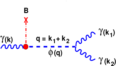
Figure 1: The Feynman diagram describing the contribution to the photon splitting amplitude in an external magnetic field. The spin-0 particle $(\phi)$ is coupled to two-photons as in Eq. (1). The dashed horizontal line indicates the propagator of the spin-0 particle, and the vertical dot-dashed line stands for the external magnetic field insertion. The bubble represents the magnetic form factor; $k$, $q$, and $k_{1,2}$ denote, respectively, the initial, intermediate and final four-momenta.

Consider therefore the process illustrated in Fig. 1, i.e. $\gamma(k)\to\gamma(k_{1})\,\gamma(k_{2})\,$, where $k$ and $k_{1,2}$ are, respectively, the four momenta of the initial and of the final photons. Suppose also that the photons exchange momentum with the external magnetic field (represented by a cross in Fig.1) which is assumed to be static (i.e. time-independent) but spatially inhomogeneous. Consequently, while the total energy of the reaction is conserved (owing to the time-independence of the external field), the three-momentum can be absorbed by the (inhomogeneous) external field.

Defining the four momenta of the final photons as $k_{1}=(\omega_{1},\vec{k}_{1})$ and $k_{2}=(\omega_{2},\vec{k}_{2})$, the differential cross section for the scattering of a photon by a time-independent external field is:

$$d\sigma=\,\frac{1}{2}\,\sum_{\rm pol}|{\rm M}(\gamma\to\gamma\gamma)|^{2}\,(2\pi)\delta(\omega-\omega_{1}-\omega_{2})\,\frac{1}{2\omega}\frac{d^{3}\vec{k}_{1}}{2\omega_{1}(2\pi)^{3}}\frac{d^{3}\vec{k}_{2}}{2\omega_{2}(2\pi)^{3}},$$ (2)

where ${\rm M}(\gamma\to\gamma\gamma)$ is the matrix element of the process and the $1/2$-factor arises since the photons of the final state are indistinguishable. According to Fig. 1 the scattering amplitude for $\gamma\to\gamma\gamma$ in a magnetic field can be written as

$${\rm M}(\gamma\to\gamma\gamma) = \frac{\sin{\theta}}{\Lambda}\omega\,\hat{{\rm B}}(\vec{p})\,\frac{i}{(k_{1}+k_{2})^{2}-m^{2}+i\,m\Gamma}V_{\gamma\gamma}(k_{1},k_{2})\,,$$ (3)

where $m$ and $\Gamma$ are, respectively, the mass and total width of the exchanged boson; moreover $\theta$ is the angle between the direction of the external magnetic field ${\rm\vec{B}}$ and the incoming photon three-momentum $\vec{k}$. The term $\hat{{\rm B}}(\vec{p})$ is the Fourier transform of the projection of $\vec{{\rm B}}(\vec{x})$ along the polarization vector of the incoming photon, namely $\hat{{\rm B}}(\vec{p})=\int|\vec{n}\cdot\vec{{\rm B}}(\vec{x})|\,e^{i\,\vec{p}\cdot\vec{x}}d^{3}x$, where $\vec{p}=\vec{k}-\vec{k}_{1}-\vec{k}_{2}\,$ is the momentum absorbed by the external field and $\vec{n}$ is the unit vector parallel to the direction of the incoming polarization. In Eq.(3), the term

$$V_{\gamma\gamma}(k_{1},k_{2})=\frac{1}{\Lambda}\left(k_{1}^{\mu}\,\varepsilon_{1}^{\nu}\,k_{2}^{\alpha}\,\varepsilon_{2}^{\beta}\right)\epsilon_{\mu\nu\alpha\beta}\,,$$ (4)

represents the boson-$\gamma\gamma$ vertex contribution where $\varepsilon_{1}^{\mu}(k_{1})$ and $\varepsilon_{2}^{\mu}(k_{2})$ are the polarization vectors of the two final photons and $\epsilon_{\mu\nu\alpha\beta}$ is the total antisymmetric tensor.

Inserting Eqs.(3) and (4) into Eq.(2) the differential cross-section becomes

$$d\sigma = \frac{\omega}{8\Lambda^{4}}\frac{(k_{1}+k_{2})^{4}\,\sin^{2}{\theta}}{((k_{1}+k_{2})^{2}-m^{2})^{2}+\Gamma^{2}m^{2}}|\hat{\rm B}(\vec{p})|^{2}\,$$ (5)

$$\times (2\pi)\delta(\omega-\omega_{1}-\omega_{2})\,\frac{d^{3}\vec{k}_{1}}{2\omega_{1}(2\pi)^{3}}\frac{d^{3}\vec{k}_{2}}{2\omega_{2}(2\pi)^{3}}.$$

As previously mentioned, for the reaction to proceed, the three-momentum $\vec{p}$ must be absorbed by the external magnetic field. In fact, if the external field is fully homogeneous not only in time but also in space, we will have that, in Fourier space, $|\hat{{\rm B}}(\vec{p})|\propto\delta^{(3)}(\vec{k}-\vec{k}_{1}-\vec{k}_{2})$. This occurrence demands that Eq.(5) is proportional to $(k_{1}+k_{2})^{2}\,\delta^{(4)}(k-k_{1}-k_{2})$. Then the total cross section vanishes after integrating over the total phase space.

Naively, if the magnetic field has a finite extension of order $L$ and vanishes outside of it, the translational invariance is broken and the external field could easily absorb momentum of magnitude $\sim 1/L$. To model this situation, consider, as an example, a magnetic field configuration with Cartesian components $\vec{{\rm B}}(\vec{x})=({\rm B}_{x}(\vec{x}),0,{\rm B}_{z}(\vec{x}))$, where

$${\rm B}_{z}(\vec{x})={\rm B}\,\exp\left(-\frac{x^{2}}{L^{2}}-\frac{y^{2}+z^{2}}{R^{2}}\right),\qquad{\rm B}_{x}(\vec{x})=\frac{2z}{R^{2}}\,\int_{-\infty}^{x}\,dx\,{\rm B}_{z}(\vec{x})\,.$$ (6)

It is easy to check that $\vec{{\rm B}}(\vec{x})$ is indeed solenoidal. By choosing the three-momentum $\vec{k}$ of the incoming photon along the $\hat{x}$-axis, only the $\hat{z}$ component of the magnetic field will enter Eq. (5) where $|\hat{{\rm B}}(\vec{p})|\to|\int d^{3}x{\rm B}_{z}(\vec{x})|$.

Let us then compute our main observable, i.e. the number of photon splitting events taking place inside the magnetic field. This quantity, denoted in what follows by $N_{\gamma\gamma}$, is simply the product of the cross section $\sigma$ (obtainable from Eq.(5)) times the flux of incoming photons $\Phi=N_{\gamma}(t)/A$ , i.e. $N_{\gamma\gamma}(t)=\sigma\Phi$. The quantity $N_{\gamma}(t)$ is the number of incoming photons per unit time crossing the magnetic field and $A=\pi R^{2}$ is the surface spanned by the magnetic field on the the plane orthogonal to the direction of the incoming photon momentum (in our frame the $\hat{y}-\hat{z}$ plane). Inserting now Eq.(6) into Eq.(5), the differential number of photon splitting events per unit time is given by $dN_{\gamma\gamma}(t)=N_{\gamma}(t)\,d{\rm P}(\gamma\to\gamma\gamma)$, where

$$d{\rm P}(\gamma\to\gamma\gamma) = \frac{\omega}{32\Lambda^{4}}{\rm B}^{2}\frac{(k_{1}+k_{2})^{4}}{((k_{1}+k_{2})^{2}-m^{2})^{2}+\Gamma^{2}m^{2}}\,\pi\,L^{2}\,\exp{\left(-\frac{p^{2}L^{2}}{2}\right)}\,\times$$ (7)

$$(2\pi)^{3}\delta(\omega-\omega_{1}-\omega_{2})\,\Delta_{R}(\frac{k_{1y}+k_{2y}}{\sqrt{2}})\,\Delta_{R}(\frac{k_{1z}+k_{2z}}{\sqrt{2}})\,\times$$

$$\frac{d^{3}\vec{k}_{1}}{2\omega_{1}(2\pi)^{3}}\frac{d^{3}\vec{k}_{2}}{2\omega_{2}(2\pi)^{3}}\,,$$

is the differential probability of $\gamma$ going to $\gamma\gamma$. In Eq. (7), the absorbed momentum is $p\equiv\omega-k_{1x}-k_{2x}$. The quantity $\Delta_{L}(p)$ is nothing but $\Delta_{L}(p)\equiv(L/\sqrt{\pi})\,\exp{\left(-L^{2}\,p^{2}\right)}$, which is a well known representation of the Dirac-delta function $\delta(p)$ in the limit $\lim_{L\to\infty}\Delta_{L}(p)=\delta(p)$. To simplify the problem, the shape of the magnetic field can be chosen in such a way that $R\to\infty$ while $L$ stays finite: in this way the total momentum will be absorbed only along the initial beam direction $\hat{x}$. In practice this means that $R\gg L$, i.e. $R$ much larger than the characteristic inhomogeneity scale along the $\hat{x}$ direction.

After using the Dirac-delta functions for the partial integrations a change of variables allows to write the total probability as

$${\rm P}(\gamma\to\gamma\gamma)=\frac{{\rm B}^{2}}{256\pi\Lambda^{4}}[{\mathcal{I}}_{1}(\omega)+{\mathcal{I}}_{2}(\omega)]\,,$$ (8)

where the following integrals have been introduced

$${\mathcal{I}}_{1}(\omega) = \omega\,\int_{0}^{{\frac{\omega}{2}}}\,d\omega_{1}\int_{0}^{4\omega_{1}(\omega-\omega_{1})}\,d\mu^{2}\frac{F(\mu^{2})}{\left[(\mu^{2}-m^{2})^{2}+\Gamma^{2}m^{2}\right]}\,,$$ (9)

$${\mathcal{I}}_{2}(\omega) = \omega\,\int_{\frac{\omega}{2}}^{\omega}\,d\omega_{1}\int_{0}^{2\omega(\omega-\omega_{1})}\,d\mu^{2}\frac{F(\mu^{2})}{\left[(\mu^{2}-m^{2})^{2}+\Gamma^{2}m^{2}\right]}\,,$$ (10)

$$F(\mu^{2}) = \,\frac{\mu^{4}}{\omega^{2}-\mu^{2}}\,\,L^{2}\,e^{-L^{2}\,p^{2}/2},\qquad p=\omega(1-\sqrt{1-\mu^{2}/\omega^{2}}\,).$$ (11)

The relevant physical regime for the present purposes is the one where $\omega>m$. This limit is realized, for instance, when the incident photon beam is in the optical and the scalar mass in the PVLAS range. If $m/\omega\ll 1$, the Breit-Wigner distribution can be easily integrated in the thin-resonance limit (since $\Gamma=m^{3}/(64\pi\Lambda^{2})\ll m$), and, from Eq. (8) the result is simply

$${\rm P}(\gamma\to\gamma\gamma) = \frac{{\rm B}^{2}\,\omega^{2}}{m^{4}\,\Lambda^{2}}\,\frac{\pi^{3/2}}{2\sqrt{2}}\,{\mathcal{F}}(\chi)\,{\rm BR}(\varphi_{P}\to\gamma\gamma)\,\left(1+\,{\cal O}(\frac{\Gamma}{m})\,\right),$$ (12)

$${\mathcal{F}}(\chi) = \sqrt{\frac{2}{\pi}}\,\chi^{2}e^{-\chi^{2}/2},\qquad\chi=\overline{p}\,L,$$ (13)

where ${\rm BR}(\varphi_{P}\to\gamma\gamma)=m^{3}/(64\,\pi\Lambda^{2}\,\Gamma)$ is the branching ratio of the pseudo-scalar decay in $\gamma\gamma$ and terms of order ${\cal O}(m^{2}/\omega^{2})$ have been neglected. Furthermore, in Eq. (13) $\overline{p}$ is the absorbed momentum at the resonance, i.e.

$$\overline{p}=\omega\biggl{(}1-\sqrt{1-\frac{m^{2}}{\omega^{2}}}\biggr{)}\,.$$ (14)

Note that ${\mathcal{F}}(\chi)$, being dimensionless and normalized to $1$, measures the suppression of $P(\gamma\to\gamma\gamma)$ when the magnetic inhomogeneity scale $L$ is larger than $1/\overline{p}$. The limit $\omega\gg m$ is naturally implemented for the case of PVLAS axions when $\omega$ is the energy of the (optical) photon beam, and in this case $\overline{p}\simeq m^{2}/(2\omega)$. Notice that the leading term of the integrals in Eq.(8) is proportional to $1/\Gamma$, enhancing the suppression induced by the $1/\Lambda^{4}$ coupling. In particular, when the pseudo-scalar has only the decay channel in two-photon, ${\rm BR}(\varphi_{P}\to\gamma\gamma)=1$, Eq. (12) reproduces the probability of photon conversion in on-shell axions [3]. Such an occurrence is a direct consequence of the Breit-Wigner distribution in Eq.(5). It is relevant to mention that if $\omega<m$ (which is opposite to the limit where Eq. (12) has been derived), the region of the pole in the integrand of Eqs. (9) and (10) does not contribute to the total integral. Consequently, the total probability is simply suppressed as ${\rm B}^{2}/\Lambda^{4}$.

Generalizations of the result (12) to the scalar case are possible. In the scalar case the boson-$\gamma\gamma$ vertex of Eq. (4) is different and the coupling will be dictated by $\tilde{\Lambda}$. Consequently, the relevant geometric set-up will be the one where the incoming photon polarization is orthogonal (and not parallel) to the orientation of the external magnetic field. Moreover, the dependence of the branching ratio for the decay in $\gamma\gamma$ upon the mass, couplings and width of the scalar particle has the same analytical expression as in the pseudo-scalar case. With these caveats the numerical results are the same if $\Lambda=\tilde{\Lambda}$.

According to Eq. (13), the resonant effect in Eqs. (12) is achieved when $\chi=\sqrt{2}$ corresponding to the maximum of ${\mathcal{F}}(\chi)$ as a function of $\chi$. In the case of an incident optical laser with $\omega\sim 1$ eV, and for a magnetic field of ${\mathcal{O}}(1\,{\rm Tesla})$, Eq. (12) implies that $P(\gamma\to\gamma\gamma)\simeq 4\times 10^{-14}$ for mass and coupling in the PVLAS range [6], i.e. $m\sim 10^{-3}$ eV and $\Lambda=10^{6}$ GeV. For these figures, the characteristic magnetic length $L$ will be macroscopic, i.e. $L\simeq 0.5$ m. For a Nd:Yag laser with average power of $1$ Watt (and typical wavelength of $\lambda\simeq\mu{\mathrm{m}}$), we will have that $N_{\gamma}(t)\simeq 10^{18}/s$. Consequently, the number of photon splittings per second will be $N_{\gamma\gamma}\simeq 4\times 10^{4}$ which is potentially observable.

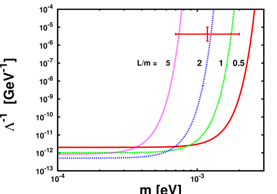
Figure 2: Exclusion regions for photon splitting (above the lines) at 95% C.L. in the $(m~{},~{}\Lambda^{-1})$ plane, for an optical beam of frequency $\omega=1$ eV, and a magnetic field ${\rm B}=1$ T of different length (L), namely L/m=0.5, 1, 2, and 5. The point with error bars corresponds to the PVLAS range. The integrated time is $10^{7}$ sec.

As it can be appreciated from Fig. 2 the PVLAS region can be excluded, at 95 % C.L. ($10^{7}$ sec of integration time), for magnetic inhomogeneity scales smaller than about a meter.

Different assumptions on the magnetic field profiles lead, up to numerical factors ${\cal O}(1)$, to the same results. This has been cross-checked with a variety of profiles where the magnetic field vanishes at infinity. Moreover, the different shapes of the magnetic field will modify the form of ${\mathcal{F}}(\chi)$ and will therefore change the suppression of the probability when the magnetic inhomogeneity scale is larger than the inverse of the resonant momentum $\overline{p}$.

It is instructive to discuss briefly the massless limit of Eq.(12). In this limit, as a consequence of the Breit-Wigner distribution (see e.g. Eq.(8) ) the resonant pole is absent and the photon splitting probability is discontinuous in the limit $m\to 0$. In the massless case, the total probability of photon splitting should then be calculated by setting $m=0$ inside the integrand of Eq.(8) and the final result can be expressed as

$$P(\gamma\to\gamma\gamma)=\frac{{\rm B}^{2}}{256\,\pi\,\Lambda^{4}}\,{\mathcal{I}}_{3}(\xi),$$ (15)

$${\mathcal{I}}_{3}(\xi)=\xi^{2}\int_{0}^{1/2}\,dx\left(\int_{0}^{4x(1-x)}\,dy+\int_{0}^{2x}\,dy\right)\frac{e^{-\xi^{2}(1-\sqrt{1-y})^{2}/2}}{1-y},$$ (16)

where $\xi=\omega\,L$. If, as previously assumed, $\omega=1$ eV and $L\simeq{\mathcal{O}}(\mathrm{m})$, we have $\xi\gg 1$, and, in this limit, ${\mathcal{I}}_{3}(\xi)\simeq\xi\,\sqrt{2\pi}$. This occurrence implies then

$$P(\gamma\to\gamma\gamma)\simeq\frac{{\rm B}^{2}\,\omega\,L}{128\,\sqrt{2\pi}\,\Lambda^{4}}\,,$$ (17)

which is very suppressed due to the fact that the resonant effect has disappeared for $m=0$. As a useful comparison we can also report the probability of conversion of a photon into a (massless) pseudo-scalar which turns out to be $P(\gamma\to\varphi_{P})={\rm B}^{2}L^{2}\,\pi/(8\Lambda^{2})$. This result follows from the same external magnetized background assumed in Eq. (6).

Of course, the aforementioned discontinuity is present if dispersion effects, associated with the self-energy corrections due to the interaction with the external field, are neglected. These effects typically cause a shift of the squared mass, i.e. $m^{2}\to\overline{m}^{2}=(m^{2}+\sqrt{m^{2}+4m_{\rm B}^{2}})/2$, where $m_{\rm B}=\sqrt{{\rm B}\omega/\Lambda}$. Corrections, of order ${\cal O}(m_{\rm B})$, arise as well for the photon self-energy. If the mass is in the PVLAS range ($m_{\rm PVLAS}\sim 10^{-3}{\rm eV}$) for Tesla magnetic fields and couplings $\Lambda\sim 10^{6}$ GeV, $m_{\rm B}\simeq 10^{-6}\,{\rm eV}\ll m_{\rm PVLAS}$ and dispersion effects are negligible for resonant photon splitting.

As already mentioned PVLAS results lack independent confirmations. In the present paper it has been shown that, for the PVLAS range of masses and couplings, an observable rate of photon splittings is expected when the external magnetic field can absorb three-momentum in a continuous way. Therefore, to confirm, in an independent channel, the PVLAS findings, resonant photon splitting represents an intriguing option.

References

• [1] R.D. Peccei and H. R. Quinn, Phys. Rev. Lett. 38, 1440 (1977) and Phys. Rev. D16, 1791 (1977).
• [2] S. Weinberg, Phys. Rev. Lett. 40, 223 (1978); F. Wilczek, Phys. Rev. Lett. 40, 279 (1978); M. Dine, W. Fischler, and M. Srednicki, Phys. Lett. B104, 199 (1981).
• [3] P. Sikivie, Phys. Rev. Lett. 51, 1415 (1983); Erratum-ibid. 52, 695 (1983); ibid. Phys. Rev. D 32 (1985) 2988.
• [4] M. Gasperini, Phys. Rev. Lett. 59, 396 (1987); D. Harari and P. Sikivie, Phys. Lett. B289, 67 (1992); G. Raffelt and L. Stodolsky, Phys. Rev. D 37, 1237 (1998).
• [5] G. Raffelt, Phys. Rept. 198, 1 (1990); M. S. Turner, Phys. Rept. 197, 67 (1990); M.I.Vysotsky, Ya.B.Zeldovich, M.Yu.Khlopov and V.M.Chechetkin, JETP Lett. 27, 502 (1978); M.Β Fairbairn, T.Β Rashba and S.Β Troitsky, arXiv:astro-ph/0610844.
• [6] E.Β Zavattini et al. [PVLAS Collaboration], Phys.Β Rev.Β Lett.Β  96, 110406 (2006).
• [7] L. Maiani, R. Petronzio, and E. Zavattini, Phys. Lett. B175, 359 (1986).
• [8] S. L. Adler, Ann. Phys. (N.Y.) 67, 599 (1971).
• [9] E. Gabrielli, K. Huitu, and S. Roy, Phys.Β Rev.Β  D 74, 073002 (2006).
• [10] H. Primakoff, Phys. Rev. 81, 899 (1951).
• [11] K. Van Bibber, N.R. Dagdeviren, S.E. Koonin, A. Kerman, H.N. Nelson, Phys. Rev. Lett. 59, 759 (1987).
• [12] R. Cameron et al., Phys. Rev. D47, 3707 (1993).