Endpoint singularities in unintegrated parton distributions

Abstract

We examine the singular behavior from the endpoint region $x\to 1$ in parton distributions unintegrated in both longitudinal and transverse momenta. We identify and regularize the singularities by using the subtraction method, and compare this with the cut-off regularization method. The counterterms for the distributions with subtractive regularization are given in coordinate space by compact all-order expressions in terms of eikonal-line operators. We carry out an explicit calculation at one loop for the unintegrated quark distribution. We discuss the relation of the unintegrated parton distributions in subtractive regularization with the ordinary parton distributions.

Parton distributions unintegrated in both longitudinal and transverse momenta are used in QCD to analyze hadron scattering problems with multiple hard scales and to describe infrared-sensitive processes. See jccrev03 ; jeppe06 ; metz for reviews and references. These distributions represent less inclusive versions of the ordinary parton distributions. Accordingly, due to the lack of complete KLN kln cancellation, they are affected by singularities from the region $x\to 1$ jccrev03 ; brodsky01 ; collsop81 corresponding to the exclusive phase-space boundary.

In traditional applications these singularities are handled by placing a cut-off on the endpoint region. The cut-off can be implemented as the Minkowski-space angle obtained by moving away from the lightcone the eikonal line in the matrix element that defines the parton density, as in korch and in the method of collsop81 , recently revisited in jiyuan ; ji06 . It can also be implemented in terms of the infrared cut-off associated with parton showering algorithms, as in Monte-Carlo event generators that make use of unintegrated densities junghgs ; lonn ; marchweb92 . But while the cut-off regularization is well-suited for leading order calculations, it makes it difficult to go beyond leading accuracy. Furthermore, with this method the connection with ordinary parton distributions and the lightcone limit are not so transparent.

A more systematic approach is based on subtractive regularization. A formulation of the subtraction method, suitable for treating eikonal-line matrix elements to all orders, is given in jccfh . In this approach the eikonal line attached to the field operator in the original matrix element remains lightlike, but the singularities are cancelled by counterterms provided by certain gauge-invariant eikonal correlators. The purpose of this paper is to study the unintegrated quark distribution using the method jccfh . To this end we analyze the structure of the endpoint singularity in coordinate space. We carry out an explicit calculation at one loop. This allows us to identify the counterterms, and provides support for an all-order operator formula with subtractive regularization. We present the analysis for the quark distribution, as this contains the main aspects of the endpoint dynamics, but this treatment can also be given in the case of the gluon distribution.

The analysis is given in terms of nonlocal operators. The techniques of balbra are used to make contact with the operator product expansion in local operators. Expressing the integral of unintegrated parton distributions in terms of ordinary distributions involves in general nontrivial coefficient functions, as discussed in jcczu for $\phi^{3}$ theory in dimension $d=6$ and in cchlett93 for the $x\to 0$ gluon density. The subtractive-method result that we find has the distinctive feature that the dependence on the regularization parameters introduced by the counterterms drops out in the integrated parton distribution.

Let us first recall the basic behavior near the endpoint for fixed transverse momentum $k_{\perp}$ and lightcone momentum fraction $x$ jccrev03 . The unintegrated quark distribution $f(x,k_{\perp})$, computed in a quark target with an infrared regulator $\rho$ jccrev03 ; brodsky01 , has the one-loop form

$$f_{(1)}(x,k_{\perp})=P_{R}(x,k_{\perp})-\delta(1-x)\,\delta(k_{\perp})\int dx^{\prime}\ dk_{\perp}^{\prime}\ P_{R}(x^{\prime},k_{\perp}^{\prime})\hskip 8.5359pt,$$ (1)

where

$$P_{R}(x,k_{\perp})\sim\alpha_{s}\left[{1\over{1-x}}\ {1\over{k_{\perp}^{2}+\rho^{2}}}+\{{\rm{regular}}\;\;\;{\rm{at}}\;\;\;x\to 1\}\right]\hskip 8.5359pt.$$ (2)

The $x\to 1$ singularity is the endpoint singularity, and is present for any $k_{\perp}$. A physical observable ${\cal O}$ is constructed by integrating $f$ against a test function $\varphi$ (specifying the final state, hard subprocess, etc.), which yields

$${\cal O} = \int dx\ dk_{\perp}\ f_{(1)}(x,k_{\perp})\ \varphi(x,k_{\perp})$$ (3)

$$= \int dx\ dk_{\perp}\ [\varphi(x,k_{\perp})-\varphi(1,0_{\perp})]\,P_{R}(x,k_{\perp})\hskip 8.5359pt.$$

While in the inclusive case, with $\varphi$ independent of $k_{\perp}$, the $x\to 1$ behavior in Eq. (3) simply corresponds to the familiar $1/(1-x)_{+}$ distribution from real/virtual cancellation, in the general case uncancelled divergences are expected from the endpoint region.

We now proceed as follows. We compute this singularity in coordinate space, we apply the subtractive regularization method jccfh , and then going back to momentum space we see the generalization of Eq. (3) associated with it.

We begin by considering the matrix element

$${\widetilde{f}}(y)={1\over 2}\ \sum_{s}\ \langle p,s|{\overline{\psi}}(y)V_{y}^{\dagger}(n)\gamma^{+}V_{0}(n)\psi(0)|p,s\rangle\hskip 8.5359pt.$$ (4)

Here the $\psi$’s are the two quark fields evaluated at distance $y=(0,y^{-},y_{\perp})$ with arbitrary $y^{-}$ and $y_{\perp}$, $p$ and $s$ are the momentum and spin of the target, taken to be a quark with $p^{\mu}=(p^{+},m^{2}/(2p^{+}),0_{\perp})$, and $V$ is the path-ordered exponential

$$V_{y}(n)={\cal P}\exp\left(ig_{s}\int_{0}^{\infty}d\tau\ n^{\mu}A_{\mu}(y+\tau\ n)\right)\hskip 8.5359pt.$$ (5)

In Eq. (5) $n$ is the direction of the eikonal line and $A$ is the gauge field, $A_{\mu}=A_{\mu}^{a}t^{a}$, with $t^{a}$ the color generators in the fundamental representation. The unintegrated quark distribution is obtained from the Fourier transform

$$f(x,k_{\perp})=\int{{dy^{-}}\over{2\pi}}{{d^{d-2}y_{\perp}}\over{(2\pi)^{d-2}}}\ e^{-ixp^{+}y^{-}+ik_{\perp}\cdot y_{\perp}}\ {\widetilde{f}}(y)\hskip 8.5359pt,$$ (6)

with $d=4-2\epsilon$ the space-time dimension.

Let us expand the matrix element (4) to one loop. In Feynman gauge, the endpoint behavior results from graphs with gluons coupling to the eikonal line, Fig. 1(a) and (b). We calculate these contributions working in dimensional regularization with dimension $d$, and regulating the collinear and soft divergences by keeping finite quark mass $m$ and gluon mass $\lambda$. We take $n$ to be lightlike, $n=(0,1,0_{\perp})$, as is the case for ordinary parton distributions, and will give later the extension of the result to $n^{2}\neq 0$. Because we work in covariant gauge we need not consider the contribution from the gauge link at infinity.

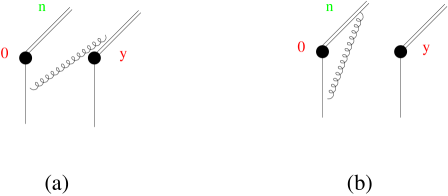
Figure 1: One-loop contributions to the quark density from eikonal-line couplings.

We expand the path-ordered exponential in Eq. (4) to first order in $gA$, and represent the gauge-field two-point correlator as

$$\langle A_{\mu}^{a}(z_{1})A_{\nu}^{b}(z_{2})\rangle=\delta^{ab}\ \int_{0}^{\infty}d\alpha\ \int{{d^{4}\ell}\over{(2\pi)^{4}}}\ d_{\mu\nu}(\ell)\ e^{i[\alpha(\ell^{2}-\lambda^{2}+i\varepsilon)+\ell\cdot(z_{2}-z_{1})]}\hskip 8.5359pt.$$ (7)

Similarly, for quarks

$$\langle\psi_{i}(z_{1}){\overline{\psi}}_{k}(z_{2})\rangle=\delta_{ik}\ \int_{0}^{\infty}d\beta\ \int{{d^{4}q}\over{(2\pi)^{4}}}\ ({\hat{q}}+m)\ e^{i[\beta(q^{2}-m^{2}+i\varepsilon)+q\cdot(z_{2}-z_{1})]}\hskip 8.5359pt.$$ (8)

We switch to new integration variables $v,\sigma$ by setting

$$\alpha=v\ \sigma\hskip 5.69046pt,\hskip 11.38092pt\beta=(1-v)\ \sigma\hskip 8.5359pt,$$ (9)

with $0\leq v\leq 1$, $0\leq\sigma<\infty$. Then the integrals in the momenta $\ell,q$ and $\tau,\sigma$ variables can be carried out explicitly for the graphs in Fig. 1 in terms of Bessel functions. We obtain

$${\widetilde{f}}_{(a)+(b)} = {{\alpha_{s}C_{F}}\over{4^{d/2-2}\pi^{d/2-1}}}\ p^{+}\int_{0}^{1}dv\ {v\over{1-v+i\varepsilon}}\ \left[e^{ip\cdot yv}\ 2^{d/2-1}\ \left({\rho^{2}\over{\mu^{2}}}\right)^{d/4-1}\ \right.$$ (10)

$$\times \left.{1\over{[(-y^{2}+i\varepsilon)\mu^{2}]^{d/4-1}}}K_{d/2-2}(\sqrt{\rho^{2}(-y^{2}+i\varepsilon)})-e^{ip\cdot y}\ \Gamma(2-{d\over 2})\ ({\mu^{2}\over\rho^{2}})^{2-d/2}\right]\ ,\hskip 25.6073pt$$

where $K$ is the modified Bessel function, $\Gamma$ is the Euler gamma function, $\mu$ is the dimensional-regularization scale, and we have defined

$$\rho^{2}=(1-v)^{2}m^{2}+v\lambda^{2}\hskip 8.5359pt.$$ (11)

The singularity for $v\to 1$ in the integrand of Eq. (10) is the endpoint singularity. From the Fourier transform (6) we see that $v$ has the meaning of plus momentum fraction $(p^{+}-\ell^{+})/p^{+}$, where $\ell^{+}$ is the gluon’s plus momentum. The $y^{-}$ integral from Eq. (6) produces a $\delta(v-x)$ in the first term on the right hand side of Eq. (10) and a $\delta(1-x)$ in the second term, thus leading to the singularity structure for $x\to 1$ schematized in Eq. (2). Eq. (10) shows in particular that the $v\to 1$ singularity is present even with finite $\lambda$ and $m$ regulating the soft and collinear regions.

We can see the relation of this result with ordinary parton distributions by expanding the answer (10) in powers of the distance $y^{2}$ from the lightcone. This step is analogous to the technique balbra to analyze nonlocal string-like operators. We use the representation of $K$

$$\left({\rho^{2}\over{-y^{2}+i\varepsilon}}\right)^{d/4-1}\ K_{d/2-2}(\sqrt{\rho^{2}(-y^{2}+i\varepsilon)})=2^{1-d/2}\ \Gamma(2-{d\over 2})\ (\rho^{2})^{d/2-2}\$$

$$\times \left[1+\sum_{k=1}^{\infty}b_{k}\left(-{{y^{2}\rho^{2}}\over 4}\right)^{k}\right]+2^{d/2-3}\Gamma({d\over 2}-2)\ (-y^{2}+i\varepsilon)^{2-d/2}\ \left[1+\sum_{k=1}^{\infty}c_{k}\left(-{{y^{2}\rho^{2}}\over 4}\right)^{k}\right],$$

with

$$b_{k}={{\Gamma(d/2-1)}\over{k!\ \Gamma(k+d/2-1)}}\hskip 5.69046pt,\hskip 11.38092ptc_{k}={{\Gamma(3-d/2)}\over{k!\ \Gamma(k+3-d/2)}}\hskip 11.38092pt.$$ (13)

Inserting Eqs. (Endpoint singularities in unintegrated parton distributions),(13) in Eq. (10) we get

$${\widetilde{f}}_{(a)+(b)} = {{\alpha_{s}C_{F}}\over{4^{d/2-2}\pi^{d/2-1}}}\ p^{+}\int_{0}^{1}dv\ {v\over{1-v+i\varepsilon}}\ \left\{\left[e^{ip\cdot yv}-e^{ip\cdot y}\right]\ \Gamma(2-{d\over 2})\ ({\mu^{2}\over\rho^{2}})^{2-d/2}\right.$$ (14)

$$+ e^{ip\cdot yv}\ 4^{d/2-2}\ \Gamma({d\over 2}-2)\ [(-y^{2}+i\varepsilon)\mu^{2}]^{2-d/2}$$

$$+ \sum_{k=1}^{\infty}{{\Gamma(2-{d/2})\ \Gamma(d/2-1)}\over{k!\ 4^{k}\ \Gamma(k+d/2-1)}}\ e^{ip\cdot yv}\ ({\rho^{2}\over\mu^{2}})^{d/2+k-2}(-y^{2}\mu^{2})^{k}$$

$$+ \left.\sum_{k=1}^{\infty}{{4^{d/2-2-k}\ \Gamma({d/2}-2)\ \Gamma(3-d/2)}\over{k!\ \Gamma(k+3-d/2)}}\ e^{ip\cdot yv}\ ({\rho^{2}\over\mu^{2}})^{k}(-y^{2}\mu^{2})^{2-d/2+k}\right\}\hskip 5.69046pt.$$

The expansion (14) separates long-distance contributions in $\ln(\mu^{2}/\rho^{2})$ and short-distance contributions in $\ln(y^{2}\mu^{2})$. The first line of Eq. (14) shows that the endpoint singularity $v\to 1$ cancels for ordinary parton distributions. At leading power the endpoint singularity is associated with the coefficient function in the second line of Eq. (14). The higher order terms in the expansion are ${\cal O}(y^{2})^{k}$, with $k\geq 1$.

Consider now $n^{2}\neq 0$ in the matrix element (4). In this case the integrals in $\tau$ and $\sigma$ are not elementary, and lead to formulas in terms of parabolic cylinder functions. The result can alternatively be given as the following integral representation,

$${\widetilde{f}}_{(a)+(b)} = {{i\ e^{-i\pi d/4}}\over{4^{d/2-3/2}\pi^{d/2-1}}}\ \alpha_{s}\ C_{F}\ (\mu^{2})^{2-d/2}\ \int_{0}^{1}dv\int_{0}^{\infty}d\tau\ e^{i\tau p\cdot n(1-v)}\int_{0}^{\infty}d\sigma\ \sigma^{1-d/2}e^{-i\sigma\rho^{2}}\hskip 11.38092pt$$ (15)

$$\times \left[\left(2\ p\cdot n\ v+{{\tau n^{2}}\over{2\sigma}}\right)p^{+}+(1-v)\ m^{2}\ n^{+}\right]$$

$$\times \left\{e^{ip\cdot y}\ e^{-in^{2}\tau^{2}/(4\sigma)}-e^{ip\cdot yv}\ e^{-i(y-n\tau)^{2}/(4\sigma)}\right\}.$$

This can be used to study the two lightcone limits $y^{2}\to 0$ and $n^{2}\to 0$. In Eq. (15) the behavior of the integrand at $v\to 1$, resulting from the $\tau$ integration over the eikonal line (see Eq. (5)), is regularized by $n^{2}\neq 0$. This is precisely the method collsop81 ; jiyuan to handle the endpoint singularity, giving a cut-off in $x$ at fixed $k_{\perp}$ of order $1-x\ \hbox{\raise 2.0pt\hbox{$>$} \kern-13.0pt\lower 3.0pt\hbox{$\sim$}}\ k_{\perp}/\sqrt{4\eta}$, where $\eta=(p\cdot n)^{2}/n^{2}$. The parton distribution obeys renormalization-group evolution equations in the cut-off parameter collsop81 ; korch ; korchangle and depends on $\eta$, also after integration over transverse momenta.

The subtractive method jccfh , which we now apply, works differently. This is reviewed in jccrev03 . The matrix element (4) is still evaluated at $n$ lightlike. It is multiplied however by vacuum expectation values of eikonal lines, which provide counterterms for the subtraction of the endpoint singularity. The counterterms contain in general both lightlike and non-lightlike eikonals. For this reason we introduce the vector

$$u^{\mu}=(u^{+},u^{-},0_{\perp})$$ (16)

and the path-ordered exponentials $V_{y}(u)$, $V_{{\bar{y}}}(u)$, where $V$ is given in Eq. (5) and ${\bar{y}}$ is the lightcone projection ${\bar{y}}=(0,y^{-},0_{\perp})$. We consider the matrix element (Fig. 2)

$${\widetilde{f}}^{\rm{(subtr)}}(y)={1\over 2}\ \sum_{s}\ {{\langle p,s|{\overline{\psi}}(y)V_{y}^{\dagger}(n)\gamma^{+}V_{0}(n)\psi(0)|p,s\rangle}\over{\langle 0|V_{y}(u)V_{y}^{\dagger}(n)V_{0}(n)V_{0}^{\dagger}(u)|0\rangle\ /\ {\langle 0|V_{{\bar{y}}}(u)V_{{\bar{y}}}^{\dagger}(n)V_{0}(n)V_{0}^{\dagger}(u)|0\rangle}}}\;,$$ (17)

where $n=(0,1,0_{\perp})$. The numerator in Eq. (17) coincides with Eq. (4). The denominator is the subtraction factor designed to cancel the endpoint singularity. Below we verify the cancellation explicitly at one loop. The subtraction factor is constructed using the technique jccfh and depends on both the lightlike eikonal in direction $n$ and the non-lightlike eikonal in the auxiliary direction $u$. The unintegrated quark distribution with subtractive regularization is obtained as the Fourier transform (6) of the matrix element (17). This distribution depends on the direction $u$. However, the dependence on $u$ cancels in Eq. (17) for $y_{\perp}=0$.

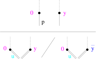
Figure 2: Coordinate-space matrix element for the quark distribution with subtraction factors.

We now go back to momentum space. We evaluate the Fourier transform (6) of Eq. (17), expanding to one loop. We introduce the regularization parameter $\zeta$, defined by the supplementary eikonal in direction $u$,

$$\zeta={p^{+2}\over 2}\ {u^{-}\over u^{+}}\hskip 5.69046pt.$$ (18)

At one loop the result from the matrix element in the numerator is of the form in Eq. (1), while the vacuum expectation values in the denominator contribute subtraction terms. Explicit calculation gives

$$\hskip 14.22636ptf^{\rm{(subtr)}}_{(1)}(x,k_{\perp}) = P_{R}(x,k_{\perp})-\delta(1-x)\,\delta(k_{\perp})\int dx^{\prime}dk_{\perp}^{\prime}P_{R}(x^{\prime},k_{\perp}^{\prime})$$ (19)

$$- W_{R}(x,k_{\perp},\zeta)+\delta(k_{\perp})\int dk_{\perp}^{\prime}W_{R}(x,k_{\perp}^{\prime},\zeta)$$

where, restoring now also the contributions of finite $(1-x)$ and including non-eikonal graphs, we have

$$P_{R}(x,k_{\perp})={{\alpha_{s}C_{F}}\over{2\pi^{2}}}\left\{{{(1-x)[(k_{\perp}^{2}+m^{2}(1-x)^{2}-2xm^{2}]}\over{[k_{\perp}^{2}+m^{2}(1-x)^{2}]^{2}}}+{{2x/{(1-x)}}\over{[k_{\perp}^{2}+m^{2}(1-x)^{2}]}}\right\}\hskip 5.69046pt,$$ (20)

and

$$W_{R}(x,k_{\perp},\zeta)={{\alpha_{s}C_{F}}\over{2\pi^{2}}}\left\{-{{8\zeta(1-x)}\over{[k_{\perp}^{2}+4\zeta(1-x)^{2}]^{2}}}+{{2/{(1-x)}}\over{[k_{\perp}^{2}+4\zeta(1-x)^{2}]}}\right\}\hskip 5.69046pt.$$ (21)

Here we have set $\lambda=0$, $d=4$. Note the endpoint singularity $(1-x)^{-1}\times\alpha_{s}C_{F}/(\pi^{2}k_{\perp}^{2})$ for $x\to 1$ in $P_{R}$, and the corresponding subtraction term in $W_{R}$. The specific form of the counterterms in the second line of Eq. (19) comes from the subtraction factors in Fig. 2. In particular, terms in $\delta(1-x)$ cancel between the vacuum expectation values in Eq. (17). This reflects the fact that in the coordinate-space results (10),(15) only the terms in $e^{ip\cdot yv}$ depend on $y_{\perp}$, while those in $e^{ip\cdot y}$ do not.

Observe that the unintegrated distribution in Eq. (19) depends on the parameter $\zeta$ of Eq. (18), but upon integration in $k_{\perp}$ the $\zeta$-dependence cancels between the two terms in the second line of Eq. (19). This implementation of the subtraction method is to be contrasted with the cut-off method collsop81 ; jiyuan , where a residual dependence on the cut-off parameter is left in the integrated distribution.

We may now consider the analogue of Eq. (3) for a physical observable $\cal O$. Similarly to Eq. (3), suppose integrating a test function $\varphi$ over the distribution $f^{\rm{(subtr)}}$. Using Eq. (19), we obtain

$${\cal O} = \int dx\ dk_{\perp}\ f^{\rm{(subtr)}}_{(1)}(x,k_{\perp})\ \varphi(x,k_{\perp})$$ (22)

$$= \int dx\ dk_{\perp}\ \left\{(P_{R}-W_{R})\ \varphi(x,k_{\perp})-P_{R}\ \varphi(1,0_{\perp})+W_{R}\ \varphi(x,0_{\perp})\right\}$$

$$= \int dx\ dk_{\perp}\ \left\{P_{R}\ [\varphi(x,0_{\perp})-\varphi(1,0_{\perp})]+(P_{R}-W_{R})\ [\varphi(x,k_{\perp})-\varphi(x,0_{\perp})]\,\right\}\hskip 5.69046pt.$$

Unlike Eq. (3), the endpoint behavior in Eq. (22) is regularized. For $x\to 1$ the first term in the last line of Eq. (22) corresponds to the $1/(1-x)_{+}$ distribution, while in the second term the endpoint singularity in $P_{R}$ is cancelled by $W_{R}$.

In conclusion, we verify at one loop that the subtractive method, implemented in Eq. (17), provides a well-prescribed technique to identify and regularize the endpoint singularities in unintegrated parton distributions. This is accomplished while keeping the eikonal in direction $n$ exactly lightlike, in contrast with approaches based on cut-off regularization collsop81 ; korch ; jiyuan ; ji06 , and canceling the singularities instead by multiplicative, gauge-invariant factors. The one-loop counterterms in Eqs. (19),(22), generated from the expansion of these factors, correspond to an extension for $k_{\perp}\neq 0$ of the plus-distribution regularization, characteristic of the inclusive case. In general, the operator expression in coordinate space given by Eq. (17) can be used to any order.

The subtractive method provides an alternative to the cut-off method, most commonly used in this context. In the cut-off method the eikonal $n$ is moved away from the lightcone, as in Eq. (15) above, and the cut-off is given by $\eta=(p\cdot n)^{2}/n^{2}$. The lightcone limit is not smooth, so that one does not simply recover the ordinary parton distribution by integrating over $k_{\perp}$ and taking $\eta\to\infty$ collsop81 . This behavior can be compared with the dependence on the “gauge-invariant cut-off” parameter (18) in the case of the subtractive method. As noted below Eq. (17) and below Eq. (21), the dependence on the non-lightlike eikonal, introduced in Eq. (16) to regularize the endpoint at unintegrated level, drops out of the distribution integrated over transverse momenta, where such regularization occurs independently by KLN cancellation.

Different methods of regularizing the endpoint singularities in the unintegrated parton distributions will result in different coefficient functions for the $y^{2}$ expansion of the kind in Eq. (14). The observed cancellation of the $\zeta$ dependence in the integrated density could be seen as corresponding to a particular scheme choice, which may be advantageous for applications such as the construction of event-generation methods jcczu ; fhproc ; bauermc . It can also be helpful for studying the re-expansion of unintegrated distributions in terms of ordinary distributions balbra ; jcczu ; cchlett93 . The possibility of constructing one such scheme appears to be a distinctive feature of the subtractive method compared to the cut-off method.

Acknowledgments. I thank V. Braun, M. Ciafaloni and J. Collins for valuable discussions.

References

- (1) J.C. Collins, Acta Phys. Polon. B 34 (2003) 3103.
- (2) J.R. Andersen et al., Eur. Phys. J. C48 (2006) 53.
- (3) A. Metz, talk at DESY Workshop, Hamburg, September 2006.
- (4) T. Kinoshita, J. Math. Phys. 3 (1962) 650; T.D. Lee and M. Nauenberg, Phys. Rev. 133 (1964) 1549.
- (5) S.J. Brodsky, D.S. Hwang, B.Q. Ma and I. Schmidt, Nucl. Phys. B593 (2001) 311.
- (6) J.C. Collins, in Perturbative Quantum Chromodynamics, ed. A.H. Mueller, World Scientific 1989, p. 573; J.C. Collins and D.E. Soper, Nucl. Phys. B193 (1981) 381.
- (7) G.P. Korchemsky, Phys. Lett. B 220 (1989) 629.
- (8) X. Ji, J. Ma and F. Yuan, Phys. Rev. D 71 (2005) 034005; JHEP 0507 (2005) 020.
- (9) P. Chen, A. Idilbi and X. Ji, Nucl. Phys. B763 (2007) 183.
- (10) H. Jung, Mod. Phys. Lett. A19 (2004) 1.
- (11) G. Gustafson, L. Lönnblad and G. Miu, JHEP 0209 (2002) 005; L. Lönnblad and M. Sjödahl, JHEP 0402 (2004) 042, JHEP 0505 (2005) 038.
- (12) G. Marchesini and B.R. Webber, Nucl. Phys. B386 (1992) 215.
- (13) J.C. Collins and F. Hautmann, Phys. Lett. B 472 (2000) 129; JHEP 0103 (2001) 016.
- (14) I.I. Balitsky and V.M. Braun, Nucl. Phys. B361 (1991) 93.
- (15) J.C. Collins and X. Zu, JHEP 0503 (2005) 059.
- (16) S. Catani, M. Ciafaloni and F. Hautmann, Phys. Lett. B 307 (1993) 147; S. Catani and F. Hautmann, Nucl. Phys. B427 (1994) 475.
- (17) G.P. Korchemsky and G. Marchesini, Phys. Lett. B 313 (1993) 433; G.P. Korchemsky and A. Radyushkin, Phys. Lett. B 279 (1992) 359.
- (18) F. Hautmann, hep-ph/0101006, in Proceedings of Linear Collider Workshop LCWS2000, Fermilab, Batavia 2000 (p.408).
- (19) C.W. Bauer and M.D. Schwartz, hep-ph/0607296.