February 2007

The Pomeron in the weak and strong coupling limits
and kinematical constraints
Anna  M.  Staśto

Physics Department, Penn State University,
104 Davey Laboratory, University Park PA 16802-6300, USA
and

Institute of Nuclear Physics PAN, Radzikowskiego 152, Kraków, Poland

()

We show that a resummation model for the evolution kernel at small $x$ creates a bridge between the weak and strong couplings. The resummation model embodies DGLAP and BFKL anomalous dimensions at leading logarithmic orders, as well as a kinematical constraint on the real emission part of the kernel. In the case of pure gluodynamics the strong coupling limit of the Pomeron intercept is consistent with the exchange of the spin-two, colorless particle.

1 Introduction

The high energy limit of QCD is one of the most important aspects of strong interactions. The abundance of precision data from high - energy colliders, like HERA and Tevatron, enables one to confront and check the theoretical predictions in QCD. The standard framework used to make the predictions in QCD is that of the collinear factorization. In this approach the hard matrix element is computed within the perturbative QCD. The collinear singularities are factorized into the parton densities which are then evolved using the renormalization group equations. These equations provide a tool for computing the change of the densities of quarks and gluons at the variable scale. Although the parton distribution evolves, the total energy-momentum is conserved. This is reflected by the fact that the anomalous dimensions of the DGLAP equations vanish at $j=\omega+1=2$

$$2N_{f}\gamma_{qg}(\omega)|_{\omega=1}+\gamma_{gg}(\omega)|_{\omega=1}=0$$

and

$$\gamma_{gq}(\omega)|_{\omega=1}+\gamma_{qq}(\omega)|_{\omega=1}=0\;,$$

order by order in the perturbation theory. Therefore parton distributions $F_{i}(x,\mu^{2})$ obey the momentum sum rule

$$\sum_{i}\int_{0}^{1}\,dx\,xF_{i}(x,\mu^{2})\;=\;1\;,$$

where $x$ is the fraction of the longitudinal momentum of the hadron carried by the parton, and $\mu$ is the scale of the DGLAP equation. In the distribution $F_{i}$ partons are on-shell and have zero transverse momentum. This by itself is already an approximation, since one does not observe free, on-shell quarks and in any hadronic process the target partons are always off-shell.

An alternative approach is BFKL resummation [1], where gluon emission diagrams are summed in the Regge limit $s\gg|t|$. The amplitude computed perturbatively in this regime has the form

$$A(s,t)\;\sim\;s^{\alpha_{P}(t)}\;,$$

where $\alpha_{P}$ is the Pomeron trajectory given by the integro-differential equation

$$\frac{df(x,k_{T})}{d\ln 1/x}\;=\;\frac{\alpha_{s}N_{c}}{\pi}\int d^{2}k_{T}^{\prime}\,K(k_{T},k_{T}^{\prime})\,f(x,k_{T}^{\prime})\;.$$ (1)

In (1) $K(k_{T},k_{T}^{\prime})$ is the BFKL kernel which depends on the transverse momenta $k_{T}$. In the leading logarithmic approximation the Pomeron trajectory intercept equals

$$\alpha_{P}(0)\,=\,1+4\ln 2\,\frac{N_{c}\alpha_{s}}{\pi}\;.$$

The solution to Eq. (1) is the unintegrated gluon distribution function $f(x,k_{T})$, which still contains the information about the transverse momentum of the gluon. The distribution $f$ is for the off-shell gluons.

The next-to-leading order corrections [2, 3] dominate the leading order. Consequently, several methods on the resummation of the perturbative series were developed, to name [4]-[9], [10]-[15], [16] and [17]. There is, as yet unfortunately, no unique resummation procedure at small $x$. However, the major building blocks are common to all approaches, like the DGLAP anomalous dimension, kinematical constraints, running coupling and the momentum sum rule.

The unique sum of the perturbation theory, if it exists, should contain the complete information about the anomalous dimensions. It is then legitimate to ask what is the strong coupling limit of such a sum. While one does not yet have a complete solution, one can still build models and explore them in the strong coupling limit. In [18, 19] a resummation procedure was proposed and it revealed that the intercept in the limit of the infinite coupling equals one. In this paper we investigate the details of the behavior of the BFKL eigenvalue restricted by the kinematical constraint and the momentum sum rule. We show that in the limit $\alpha_{s}\rightarrow\infty$ the intercept of the resummed Pomeron becomes exactly one. This is consistent with the exchange of the (possibly massless) particle of spin two. The model proposed here explains the strong coupling limit but also allows to interpolate between small and large values of $\alpha_{s}$. The importance of the exact kinematics for the parton distributions in Monte Carlo generators has been already emphasized [20, 21]. The systematic program of the definition of the collinear factorization with exact kinematics is under way [22]. This paper solely focuses on the BFKL Pomeron.

Our results may bear some relevance in the context of the string/gauge duality conjecture proposed by Maldacena [23]. Recent string theory results [24] (see also [25, 26]) showed that the scattering amplitudes in the Regge regime at large N and for the vanishing beta function exhibit a diffusion in the fifth dimension of the curved ${\rm AdS}_{5}$ space. The kernel has the form

$$K(r,r^{\prime},s)\;=\;\frac{s^{j_{0}}}{\sqrt{4\pi D\ln s}}e^{-(\ln r-\ln r^{\prime})^{2}/(4D\ln s)}\;,$$

with

$$j_{0} = 2-\frac{2}{\sqrt{\lambda}}+{\cal O}(1/\lambda)\;,$$

$$D = \frac{1}{2\sqrt{\lambda}}+{\cal O}(1/\lambda)\;,$$

where $\lambda=R^{4}/\alpha^{\prime 2}$, $R$ is the radius of the ${\rm AdS}_{5}$ space and the string tension equals $1/(2\pi\alpha^{\prime})$. In the case of the supersymmetric Yang-Mills theory $\lambda=g^{2}N=4\pi\alpha_{s}N$. Therefore the diffusion properties of the BFKL Pomeron are universal at all values of the strong coupling. We show that the resummed eigenvalue is consistent with the results of [24].

2 BFKL evolution and higher order corrections

In the leading logarithmic approximation the BFKL evolution equation [1] in the momentum representation reads

$$f(x,k_{T})=f^{(0)}(x,k_{T})\;+\\ \;+\,\frac{\alpha_{s}N_{c}}{\pi}\,\int_{x}^{1}\frac{dz}{z}\,\int\frac{k_{T}^{2}dk_{T}^{\prime 2}}{k_{T}^{\prime 2}}\,\bigg{\{}\frac{f(\frac{x}{z},k_{T}^{\prime})-f(\frac{x}{z},k_{T})}{|k_{T}^{\prime 2}-k_{T}^{2}|}\,+\,\frac{f(\frac{x}{z},k_{T})}{[4k_{T}^{\prime 4}+k_{T}^{4}]^{1/2}}\bigg{\}}\;,$$ (2)

where $x$ is the Bjorken variable, and $k_{T},k_{T}^{\prime}$ are transverse momenta of the exchanged gluons. For the unintegrated gluon distribution function $f(x,k_{T})$ the solution to the Eq. (2) behaves as

$$f\sim x^{-\omega_{P}}\;,$$ (3)

where

$$\omega_{P}\,\equiv\,\alpha_{P}(0)-1\,=\,4\ln 2\,\frac{\alpha_{s}N_{c}}{\pi}\,=\,\chi_{0}(\gamma=1/2)\;,$$ (4)

and the kernel eigenvalue $\chi_{0}$ has the form

$$\chi_{0}(\gamma)\;=\;-2\gamma_{E}-\psi(\gamma)-\psi(1-\gamma)\;,$$ (5)

where $\psi$ is the digamma function and $\gamma$ is the Mellin conjugate to $\ln k_{T}^{2}$. The next-to-leading corrections to the BFKL equation are known to be very large [2, 3]. The resummation procedure yields a stable result for the intercept. The following features are common to all methods of resummation

• Full DGLAP anomalous dimension (at least in the leading order of perturbation theory).

• Kinematical constraint imposed onto the gluon emission term (explained below).

• Running coupling constant.

• Momentum sum rule.

It has been shown, [12] that the Pomeron intercept computed from the renormalization group-improved BFKL equation with modifications mentioned above, is much smaller than the leading logarithmic value. The resummed value increases with the coupling constant. The $\alpha_{s}^{2}$ correction which comes from the expansion of the resummed result coincides with the NLLx [2, 3] calculation down to a couple of percent.

The kinematical constraint [27, 28, 29] (for Monte Carlo results within dipole picture see [30, 31]) is imposed onto the BFKL equation as a requirement that the virtualities of the exchanged gluons are dominated by the transverse components of the momenta. The form of the kinematical constraint depends on the scales in the scattering process [32]. For DIS reaction which is characterized by a large difference of scales of the scattered particles (where virtuality of the photon $Q^{2}$ is much larger than the scale on the proton side $\sim\Lambda_{QCD}^{2}$) the kinematical constraint imposed onto the real emission term in (2) approximately equals

$$k_{T}^{\prime 2}\,\leq\,\frac{k_{T}^{2}}{z}\;.$$ (6)

In the case of the scattering of objects with similar scales (as for example in $\gamma^{*}\gamma^{*}$ scattering with photons having both large and comparable virtualities), the kinematical constraint has a symmetrical form

$$\Theta[k_{T}/z-k_{T}^{\prime}]\,\Theta[k_{T}^{\prime}/z-k_{T}]\;.$$ (7)

The exact form of the constraint, as it appeared in [27, 28], actually is

$$q_{T}^{2}\,\leq\,k_{T}^{2}\,\frac{1-z}{z}\;,\hskip 28.45274ptq_{T}\,\equiv\,k_{T}-k^{\prime}_{T}\;.$$ (8)

In the limit of small $z$ we neglect it in the numerator of (8) and set $k_{T}^{\prime 2}\simeq q_{T}^{2}$. The comparison between the two alternative versions of the constraint (6) and (8) is relegated to the final section of this paper.

More exact analysis of the kinematics and the constraint can be best illustrated by the following simple example. In Fig. 1 we show a $2\rightarrow 3$ process with one particle emission. The details of the matrix element are irrelevant for the purpose of this discussion. The incoming momenta of the particles satisfy the condition $p_{1}^{2}\simeq p_{2}^{2}\simeq m^{2}\ll s$. The general expression for the phase space of such a diagram is

$$\int\,dPS_{3}\equiv\int\frac{d^{4}k_{1}}{(2\pi)^{4}}\frac{d^{4}k_{2}}{(2\pi)^{4}}\,\delta((k_{1}-k_{2})^{2})\,\delta((p_{1}-k_{1})^{2})\,\delta((p_{2}+k_{2})^{2})\,.$$ (9)

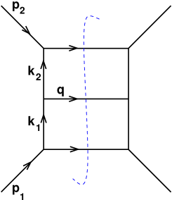
Figure 1: Elementary diagram for the one particle emission in the high energy scattering.

We decompose the exchanged particle momenta in terms of Sudakov variables
$k_{i}=(\alpha_{i}p_{1}^{+},\beta_{i}p_{2}^{-},k_{iT})$. The phase space can be rewritten as

$$\int\,dPS_{3}\equiv\frac{s^{2}}{4(2\pi)^{8}}\int d\alpha_{1}d\beta_{1}d^{2}k_{1T}\,d\alpha_{2}d\beta_{2}d^{2}k_{2T}\cdot\delta\left(s(\alpha_{1}-\alpha_{2})(\beta_{1}-\beta_{2})-(k_{1T}-k_{2T})^{2}\right)\\ \cdot\,\delta(-s(1-\alpha_{1})\beta_{1}-k_{1T}^{2})\,\delta(s(1+\beta_{2})\alpha_{2}-k_{2T}^{2})\;.$$ (10)

In the limit of the multi-Regge kinematics

$$0\ll\alpha_{2}\ll\alpha_{1}\ll 1\;,\hskip 14.22636pt0\ll|\beta_{1}|\ll|\beta_{2}|\ll 1\;,$$

which leads to the following approximated form for the phase space

$$\int\,dPS_{3}\equiv\frac{s^{2}}{4(2\pi)^{8}}\int d\alpha_{1}d\alpha_{2}d\beta_{1}d\beta_{2}\,d^{2}k_{1T}\,d^{2}k_{2T}\,\\ \cdot\,\delta\left(s\,\alpha_{1}\,\beta_{2}+(k_{1T}-k_{2T})^{2}\right)\,\delta(-s\beta_{1}-k_{1T}^{2})\,\delta(s\alpha_{2}-k_{2T}^{2})\,\;.$$ (11)

Furhermore, in the high energy limit the transverse momenta are approximated as $k_{1T}^{2}\simeq k_{2T}^{2}\simeq m^{2}$ which leads to

$$\int\,dPS_{3}\equiv\frac{1}{4(2\pi)^{8}}\int_{\alpha_{2}}^{1}\frac{d\alpha_{1}}{\alpha_{1}}\,d\alpha_{2}\,\delta(s\alpha_{2}-k_{2T}^{2})\,d^{2}k_{1T}\,d^{2}k_{2T}=\frac{1}{4(2\pi)^{8}s}\ln\frac{s}{m^{2}}\,\int\,d^{2}k_{1T}\,d^{2}k_{2T}\;.$$ (12)

Phase space becomes completely factorized into transverse and longitudinal components. This is also transparent in Eq. (2), where we identify $x\equiv m^{2}/s,\alpha_{1}\equiv x/z$. From the point of view of the leading logarthmic accuracy. i.e. $(\alpha_{s}\ln s/m^{2})^{n}$, the choice of $m^{2}$ is irrelevant since it has to be much smaller than the very large energy $s$. This, however, leads to a mismatch in the kinematics for the outgoing particle. The approximated phase space is now completely factorized, as in Eq. (12), and the $k_{T}$ integration is unrestricted. This can give an unphysical result for the emitted gluon since it can be off-shell

$$z\rightarrow 1 \longrightarrow q^{+}\rightarrow 0\;,$$

$$q^{2}=2q^{+}q^{-}-q_{T}^{2} \simeq -q_{T}^{2}<0\;{\rm if}\;k_{T}\neq k_{T}^{\prime}\;.$$ (13)

The kinematical constraint (8) guarantees that in the limit $z\rightarrow 1$ the emitted gluons are soft and on-shell ( $q^{2}\simeq 2q^{+}q^{-}\simeq q_{T}^{2}\simeq 0$). Note that the condition (8) constrains only the phase space. The matrix element is kept in the same, high-energy approximation.

3 BFKL with kinematical constraint

Let us now explore the details of the effects of the symmetrical kinematical constraint (7) imposed on the BFKL kernel. Throughout this analysis we will keep the strong coupling fixed. The modified equation reads

$$f(x,k_{T}^{2})=f^{(0)}(x,k_{T}^{2})\;+\\ \;+\,\bar{\alpha}_{s}\,\int_{x}^{1}\frac{dz}{z}\,\int\frac{k_{T}^{2}dk_{T}^{\prime 2}}{k_{T}^{\prime 2}}\bigg{\{}\frac{f(\frac{x}{z},k_{T}^{\prime 2})\Theta(k_{T}^{\prime}-k_{T}z)\Theta(k_{T}/z-k_{T}^{\prime})-f(\frac{x}{z},k_{T}^{2})}{|k_{T}^{\prime 2}-k_{T}^{2}|}+\\ +\;\frac{f(\frac{x}{z},k_{T}^{2})}{[4k_{T}^{\prime 4}+k_{T}^{4}]^{1/2}}\bigg{\}}\;,$$ (14)

where we introduced standard notation $\bar{\alpha}_{s}\equiv\alpha_{s}N_{c}/\pi$. We perform the following change of the variables

$$\eta = \bar{\alpha}_{s}\ln\frac{1}{z}\;,$$

$$\xi = \bar{\alpha}_{s}\ln\frac{1}{x}\;,$$ (15)

after which the equation (14) can be rewritten as

$$f(\xi,k_{T}^{2})=f^{(0)}(\xi,k_{T}^{2})\;+\\ \;+\,\int_{0}^{\xi}d\eta\,\int\frac{k_{T}^{2}dk_{T}^{\prime 2}}{k_{T}^{\prime 2}}\bigg{\{}\frac{f(\eta-\xi,k_{T}^{\prime 2})\,\Theta[k^{\prime}-k\exp(-\eta/\bar{\alpha}_{s})]\,\Theta[k_{T}\exp(\eta/\bar{\alpha}_{s})-k_{T}^{\prime}]-f(\eta-\xi,k_{T}^{2})}{|\,k_{T}^{\prime 2}-k_{T}^{2}\,|}+\\ +\;\frac{f(\eta-\xi,k_{T}^{2})}{[\,4k_{T}^{\prime 4}+k_{T}^{4}\,]^{1/2}}\bigg{\}}\;.$$ (16)

The LO BFKL is recovered when the theta functions are set to one and its solution can be written in a form of series in $\xi$

$$f^{LO}(\xi,k_{T}^{2})\;=\;\sum_{i}\xi^{i}\,c_{i}(k_{T}^{2})\;,$$

which is the leading logarithmic series in $\alpha_{s}\ln 1/x$. Clearly, the non-perturbative nature of the kinematical constraint is evident because of the appearance of the exponential factors $\exp(\pm\eta/\bar{\alpha}_{s})$. It is non-perturbative in a sense that the leading logarithmic expansion in $\eta$ is accompanied by the arbitrary powers in $\bar{\alpha}_{s}$. The resummed Eq. 16 contains all powers of $\bar{\alpha}_{s}$ as well as $\xi$ and the solution is a function of three variables $f(\xi,\bar{\alpha}_{s},k_{T}^{2})$, or $f(x,\bar{\alpha}_{s},k_{T}^{2})$.

For the fixed values of $\eta$ variable the $\Theta$ functions have the following behavior

$$\Theta[k_{T}^{\prime}-k_{T}\exp(-\frac{\eta}{\bar{\alpha}_{s}})]\,\Theta[k_{T}\exp(\frac{\eta}{\bar{\alpha}_{s}})-k_{T}^{\prime}] \stackrel{{\scriptstyle\alpha_{s}\rightarrow 0}}{{\longrightarrow}} 1\;,$$ (17)

$$\Theta[k_{T}^{\prime}-k_{T}\exp(-\frac{\eta}{\bar{\alpha}_{s}})]\,\Theta[k\exp(\frac{\eta}{\bar{\alpha}_{s}})-k_{T}^{\prime}] \stackrel{{\scriptstyle\alpha_{s}\rightarrow\infty}}{{\longrightarrow}} \frac{2\eta}{\bar{\alpha}_{s}}\delta(k_{T}-k_{T}^{\prime})\;.$$ (18)

The constraint breaks down the complete factorization between the longitudinal and transverse components of the momenta in the evolution. The evolution equation cannot be written any longer in a simple form of the differential equation with the factorized $\ln 1/x$ dependence as in Eq. 1.

The Mellin transform of the kernel in Eq. (14) reads

$$\chi(\gamma,\omega)\;=\;\int_{0}^{1}\frac{dz}{z}z^{\omega}\,\int\frac{k_{T}^{2}dk_{T}^{\prime 2}}{k_{T}^{\prime 2}}\bigg{\{}\frac{\Theta(k_{T}^{\prime}-k_{T}z)\,\Theta(k_{T}/z-k^{\prime})\left(\frac{k^{{}^{\prime}2}}{k_{T}^{2}}\right)^{\gamma}-1}{|\,k_{T}^{\prime 2}-k_{T}^{2}\,|}+\;\frac{1}{[\,4k_{T}^{\prime 4}+k_{T}^{4}\,]^{1/2}}\bigg{\}}=\\ \\ =\,\int_{0}^{1}\frac{dz}{z}z^{\omega}\left[u^{\omega/2}\int_{0}^{1}\frac{du}{u}\frac{u^{\gamma}-1}{1-u}+u^{-\omega/2}\int_{0}^{1}\frac{du}{u}\frac{u^{\gamma}-1}{u-1}+\int_{0}^{\infty}\frac{du}{u}\frac{1}{\sqrt{4u+1}}\right]=\\ \\ =\;\;\;-2\gamma_{E}-\psi(\gamma+\frac{\omega}{2})-\psi(1-\gamma+\frac{\omega}{2})\;.$$ (19)

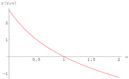
Figure 2: The behaviour of the eigenvalue function $\chi(\gamma,\omega)$ , Eq. 19, at $\gamma=1/2$ and around $\omega=1$.

The effect of the kinematical constraint is to shift the arguments of the digamma functions. The arguments $\gamma+\omega/2$ and $1-\gamma+\omega/2$ can now be equal or larger than $1$ in the domain $0<\gamma<1,\,\omega>0$. Therefore, both BFKL branches, $\psi(1)-\psi(\gamma+\omega/2)$ and $\psi(1)-\psi(1-\gamma+\omega/2)$, have zeros in this regime. This results in a solution $\chi\left(\gamma_{0},\omega_{0}(\gamma_{0})\right)=0$ with $0<\gamma_{0}<1$. In particular, the eigenvalue $\chi(\gamma,\omega)$ (19) vanishes when $\gamma\rightarrow 1/2$ and $\omega\rightarrow 1$

$$\chi(\gamma=1/2,\omega=1)\;=\;0\;,$$ (20)

which is illustrated in Fig. 2. The solution to the eigenvalue equation

$$\omega\;=\;\bar{\alpha}_{s}\,\chi(\gamma,\omega)\;,$$ (21)

can be symbolically written as [13]

$$\omega\;=\;\chi^{\rm eff}(\gamma,\bar{\alpha}_{s})\;.$$ (22)

It is difficult to obtain the solution analytically, however we can easily solve numerically for $\chi^{\rm eff}$. In Fig. 3 we illustrate this solution as a function of $\gamma$ for different values of $\bar{\alpha}_{s}$. For increasing values of $\bar{\alpha}_{s}$, the minimum of $\chi^{\rm eff}$ at $\gamma=1/2$ approaches the limit of $1$ as is expected from Eq. 20. The shape of the function changes very little with the increase of $\bar{\alpha}_{s}$. The derivative of $\chi(\gamma,\omega)$ at $\omega=1$ equals

$$\frac{d\chi(\gamma=1/2,\omega)}{d\omega}|_{\omega=1}\;=\;-\frac{\pi^{2}}{6}\;.$$ (23)

Therefore, we can write an expansion of the eigenvalue (21) around $\omega=1$

$$\chi(\gamma=1/2,\omega)\;\simeq\;(1-\omega)\frac{\pi^{2}}{6}\;,$$ (24)

however, the shifted kernel eigenvalue is not sufficient to reproduce the full NLLx BFKL result.   Motivated by the resummation procedure proposed in [12, 13] let us consider the resummed model for the eigenvalue equation in the form

$$\frac{1}{\bar{\alpha}_{s}}\;=\;\bigg{[}\frac{1}{\omega}+A(\omega)\bigg{]}\,\chi(\gamma,\omega)\;.$$ (25)

The expression in the square brackets is the LO DGLAP anomalous dimension

$$\gamma^{(0)}(\omega)\;=\;\frac{1}{\omega}+A(\omega)\;,$$ (26)

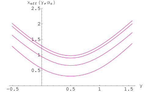
Figure 3: The solution to the eigenvalue equation (22) in the case of the LO BFKL, with kinematical constraint in the form of the function $\chi^{\rm eff}(\gamma,\alpha_{s})$, for four different values of the strong coupling: $\bar{\alpha}_{s}=0.2,\,1.0,\,5.0,\,20.0$, from the bottom to the top curve.

$$A(\omega)\;=\;-\frac{1}{\omega+1}+\frac{1}{\omega+2}-\frac{1}{\omega+3}-\psi(2+\omega)-\gamma_{E}+\frac{11}{12}\;,$$ (27)

with

$$A(0)\;=\;-\frac{11}{12}\;,$$ (28)

and

$$\gamma^{(0)}\,=\,0\;\;\;\leftrightarrow\;\;\;A(1)\,=\,-1\;.$$ (29)

The last condition, expressed by formulae (29), is the momentum sum rule in the absence of quarks $N_{f}=0$. Therefore, the resummed model (25) contains DGLAP anomalous dimension at to leading order in $\alpha_{s}\ln Q^{2}$, BFKL eigenvalue at the leading order in $\ln 1/x$ and the kinematical constraint. We again stress, that the coupling constant is fixed in this analysis. In particular, this enables us to use simple expressions for the eigenvalue conditions like Eq. (21). We expand the DGLAP anomalous dimension $\gamma^{(0)}(\omega)$ around $\omega=1$ and get

$$\gamma^{(0)}\;\simeq\;(1-\omega)\bigg{(}\frac{\pi^{2}}{6}-\frac{65}{144}\bigg{)}\;=\;1.1935\,(1-\omega)\;.$$ (30)

Using (24) and (30) we can thus write (25)

$$\frac{1}{\bar{\alpha}_{s}}\;=\;(1-\omega)^{2}\,\frac{\pi^{2}}{6}\,\bigg{(}\frac{\pi^{2}}{6}-\frac{65}{144}\bigg{)}\;=\;1.9633\,(1-\omega)^{2}\;.$$ (31)

Solving for $\omega$ we obtain

$$\omega\;=\;1-\frac{c_{0}}{\sqrt{\bar{\alpha}_{s}}}\;,$$ (32)

where

$$c_{0}\;=\;1/\sqrt{\frac{\pi^{2}}{6}\bigg{(}\frac{\pi^{2}}{6}-\frac{65}{144}\bigg{)}}\;=\;0.509346\;.$$ (33)

The result (32) should be compared with the calculation of the first correction to the intercept of the graviton presented in [24],

$$j=\,1+\omega\,=\,2-\frac{c_{0}}{\sqrt{\bar{\alpha}_{s}}},\hskip 28.45274ptc_{0}=1/\pi\;,$$

and the SUSY result [19]. The coefficient $c_{0}$ obtained from the model (25) is different, due to different details of the resummation model and the fact that here we are considering fixed coupling QCD, whereas Refs. [24, 19] apply to the SUSY YM case. However, the overall agreement is satisfactory.

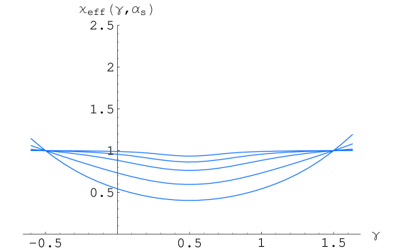
Figure 4: The solution to the eigenvalue equation (22) in the case of the LO BFKL with kinematical constraint and the DGLAP anomalous dimension in the form of the function $\tilde{\chi}^{\rm eff}(\gamma,\alpha_{s})$ for the five different values of the strong coupling $\bar{\alpha}_{s}=0.2,\,1.0,\,5.0,\,20.0,\,100.0$ from the bottom to the top curve.

The model (25) provides not only the correct limits at small and large values of the coupling but also smoothly interpolates between these limiting regions. From (31) it is clear that the $1/\sqrt{\bar{\alpha}_{s}}$ behaviour is a results of the double zero of the model (25) at $\omega=1$. The numerical solution to the equation (25) in the form of

$$\omega=\tilde{\chi}^{\rm eff}(\gamma,\alpha_{s})\;,$$

is plotted in Fig.4 where we show it for various values of the coupling constant. The fixed points in the $(\gamma,\omega)$ plane, namely $(-1/2,1)$ and $(3/2,1)$, result from the superposition of the zero $\omega=1$ and the simple poles at $\gamma+\omega/2$ and $1-\gamma+\omega/2$. The second derivative $\frac{d^{2}\tilde{\chi}^{\rm eff}(\gamma,\alpha_{s})}{d\gamma^{2}}|_{\gamma=1/2}$ appreciably changes in this case, exhibiting $1/\alpha_{s}$ behaviour at large $\alpha_{s}$. This is different from the AdS/CFT correspondence result which as well produces $1/\sqrt{\alpha_{s}}$ for the second derivative. We think that this is an artifact of the simplified model which we are considering. The overall qualitative behavior of $\tilde{\chi}^{\rm eff}$ is nonetheless consistent with the expectation from string theory side, in particular when we compare with the Fig. 2 in Ref. [24]. The effective eigenvalue has two fixed points (the points which do not change when the coupling is varied) and it can be approximated by the parabola with a minimum at $\gamma=1/2$. When the coupling is increased, the second derivative decreases. This continues until the limit of $\alpha_{s}=\infty$ is reached, and the effective eigenvalue tends to a constant equal to one.

When we compare the solutions presented in Fig. 3 and Fig. 4, we see a qualitatively different behavior of the effective eigenvalue function. In Fig. 3 the function $\chi^{\rm eff}$ is 1 only at a single point in $\gamma=1/2$. In Fig. 4 the effective eigenvalue function $\tilde{\chi}^{\rm eff}$ has a constant limit when $\bar{\alpha}_{s}\rightarrow\infty$ for all values of $\gamma$, which is the consequence of the fact that $1+\omega A(\omega)\sim(1-\omega)$ at $\omega=1$.

From $\tilde{\chi}^{\rm eff}(\gamma,\bar{\alpha}_{s})$ one can compute the dependence of the Pomeron intercept $\omega_{P}=\tilde{\chi}^{\rm eff}(1/2,\bar{\alpha}_{s})\;,$ on the coupling $\bar{\alpha}_{s}$ which we illustrate in Fig. 5 compared with the first order expansions around $\bar{\alpha}_{s}\sim 0$ (leading logarithmic BFKL [1]) and $\bar{\alpha}_{s}\sim\infty$ (the string theory in the curved background [24]).

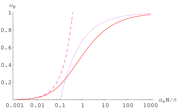
Figure 5: The strong coupling dependence of the Pomeron intercept in the case of fixed coupling. Comparison of the predictions of the resummed model with LO DGLAP (25) (solid line) to the first order results in QCD [1] (dashed line at small couplings ) and strings in curved background (dotted line at large coupling) [24]. Note the logarithmic horizontal axis for the coupling $\bar{\alpha}_{s}=\frac{\alpha_{s}N_{c}}{\pi}$.

It is also interesting to examine the convergence properties of the resummed model at small and large values of $\bar{\alpha}_{s}$. The coefficients of the expansion for the intercept $\omega_{P}=\tilde{\chi}^{\rm eff}(1/2,\bar{\alpha}_{s})$ are collected in Table 1. The left column contains the first five coefficients of the series for the Pomeron intercept at small values of $\bar{\alpha}_{s}$

$$\omega_{P}=\sum_{n\geq 1}\,a_{n}\,\bar{\alpha}_{s}^{n}\;,$$

and the right column contains the first five coefficients of the series at large values of $\alpha_{s}$

$$\omega_{P}=1-\sum_{n\geq 1}\,b_{n}\,\frac{1}{{\bar{\alpha}_{s}}^{n/2}}\;.$$

The coefficients in the small coupling expansion grow with increasing order as $a_{n+1}/a_{n}\simeq-10$ signalling the possible lack of convergence of this model at $\bar{\alpha}_{s}\rightarrow 0$. At large values of the coupling the coefficients behave at least as $b_{n+1}/b_{n}\sim 1/n$.

$a_{n}$	$b_{n}$
2.77	0.713685
-20.72	0.300767
226.69	0.085747
-3000.73	0.015120
44267.30	0.000863

Table 1: Numerical values of the expansion coefficients of the intercept at small (left column) and large (right column) values of the strong coupling constant $\bar{\alpha}_{s}$.

4 Improved kinematical constraint

It is interesting to investigate the changes to the evolution kernel when imposing more stringent kinematical constraint. In [28] it was shown that the more accurate version of the kinematical constraint has actually the form

$$q_{T}^{2}<k_{T}^{2}\,\frac{1-z}{z}\;.$$ (34)

It reduces to Eq. (6) when $z\ll 1$. Let us first consider the collinear approximation to the BFKL kernel

$$f(x,k_{T}^{2})=f^{(0)}(x,k_{T}^{2})\,+\,\int_{x}^{1}\frac{dz}{z}\left[\int^{k_{T}^{2}}\frac{dk_{T}^{\prime 2}}{k_{T}^{\prime 2}}+\int_{k_{T}^{2}}\frac{k_{T}^{2}dk_{T}^{\prime 2}}{k_{T}^{\prime 4}}\right]f(x/z,k_{T}^{\prime 2})\;,$$ (35)

and keep the $(1-z)$ term in the numerator of the kinematical constraint replacing however $q_{T}^{2}\simeq k_{T}^{\prime 2}$. This constraint also divides the domains of the integration over the longitudinal variable $z$. There are three distinct regions. For large values of $z>1/2$, $(1-z)/z<1$ and $k_{T}^{\prime 2}<k_{T}^{2}$ we have

$$\chi^{coll,l}_{z>1/2}(\gamma,\omega)\;=\;\int_{0}^{1}\frac{dz}{z}z^{\omega}\int^{k_{T}^{2}}_{0}\frac{dk_{T}^{\prime 2}}{k_{T}^{\prime 2}}\left(\frac{k_{T}^{\prime 2}}{k_{T}^{2}}\right)^{\gamma}\,\Theta(k_{T}^{2}(1-z)/z-k_{T}^{\prime 2})\,\Theta(z-1/2)\;=\\ =\;\frac{1}{\gamma}\,\beta_{1/2}(1+\gamma,\omega-\gamma)\;=\;\frac{1}{\gamma(1+\gamma)}\;{}_{2}F_{1}(1+\gamma,1+\omega;2+\gamma;-1)\;,$$ (36)

and for the region where $k_{T}^{\prime 2}>k_{T}^{2}$ and $z<1/2,\;(1-z)/z>1$ we obtain

$${\chi}^{coll,u}_{z<1/2}(\gamma,\omega)\;=\;\int_{0}^{1}\frac{dz}{z}z^{\omega}\int^{\infty}_{k_{T}^{2}}\frac{k_{T}^{2}dk_{T}^{\prime 2}}{k_{T}^{\prime 4}}\left(\frac{k_{T}^{\prime 2}}{k_{T}^{2}}\right)^{\gamma}\,\Theta(k_{T}^{2}(1-z)/z-k_{T}^{\prime 2})\,\Theta(1/2-z)=\\ =\;\frac{1}{\omega}\,\beta_{1/2}(1-\gamma+\omega,\gamma-1)\;=\;\frac{1}{\omega(1-\gamma+\omega)}\;{}_{2}F_{1}(1-\gamma+\omega,-\omega;2-\gamma+\omega;-1)\;,$$ (37)

and finally $z<1/2,k_{T}^{\prime}<k_{T}$

$${\chi}^{coll,l}_{z<1/2}(\gamma,\omega)=\int_{0}^{1}\frac{dz}{z}z^{\omega}\int^{k_{T}^{2}}_{0}\frac{dk_{T}^{\prime 2}}{k_{T}^{\prime 2}}\left(\frac{k_{T}^{\prime 2}}{k_{T}^{2}}\right)^{\gamma}\,\Theta(1/2-z)=\frac{2^{-\omega}}{\gamma\omega}\;.$$

The eigenvalue equation for (35) is then

$$1=\bar{\alpha}_{s}\left({\chi}^{coll,l}_{z>1/2}(\gamma,\omega)+{\chi}^{coll,u}_{z<1/2}(\gamma,\omega)+{\chi}^{coll,l}_{z<1/2}(\gamma,\omega)\right)\;.$$

The effect of the improved kinematical constraint on the collinear model results in the shift of the pole at $\gamma=1\rightarrow\gamma=1+\omega$. Additionaly the regularized beta functions generate the additional poles at $\gamma=-1,-2,-3,\dots$ from ${\chi}_{z>1/2}(\gamma,\omega)$ and $\gamma=2+\omega,3+\omega,\dots$ from ${\chi}_{z<1/2}(\gamma,\omega)$. These singularities are located in the same positions as those in the BFKL eigenvalue (19) with an asymmetric shift of the $\gamma$ poles. This has to be compared with the following expression

$$\frac{1}{\omega}\,\chi^{coll}(\gamma,\omega)\;=\;\frac{1}{\omega}\left(\frac{1}{\gamma}+\frac{1}{1-\gamma+\omega}\right)\;,$$ (38)

in which the small-z version of the constraint $k^{\prime 2}<k^{2}/z$ imposed onto the collinear model leads to the shift of one of the existing poles in $\gamma$ space but does not introduce any new singularities.

We next impose the constraint $q_{T}^{2}<k_{T}^{2}(1-z)/z$ in the BFKL case

$$f(x,k_{T})\;=\;f^{(0)}(x,k_{T})\,+\,\\ +\;\bar{\alpha}_{s}\,\int_{x}^{1}\frac{dz}{z}\int\frac{d^{2}k_{T}^{\prime}}{q_{T}^{2}}\left(\frac{k_{T}^{2}}{k_{T}^{\prime 2}}\,f(\frac{x}{z},k_{T}^{\prime})\,\Theta\left[k_{T}^{2}\frac{1-z}{z}-q_{T}^{2}\right]\,-\,\frac{k_{T}^{2}}{k_{T}^{\prime 2}+q_{T}^{2}}\,f(\frac{x}{z},k_{T})\right)\;.$$ (39)

In this case we perform the diagonalization of the kernel numerically. The eigenvalue $\chi(\gamma,\omega)$ as a function of $\gamma$ for different values of $\omega$ is shown in Fig. 6, where it is compared with the expression (19) for the case of the LLx BFKL with the approximated kinematical constraint. The eigenvalue is further lowered with respect to (19) but the overall differences are moderate. The most affected region is the one in the vicinity of $\gamma\rightarrow 0$. This has to be understood as an effect of the large value of $z$ in the cutoff $(1-z)/z<1$ for $z>1/2$, and therefore the cutoff becomes more stringent than the previous one in the collinear region where $k_{T}^{\prime 2}<k_{T}^{2}$.

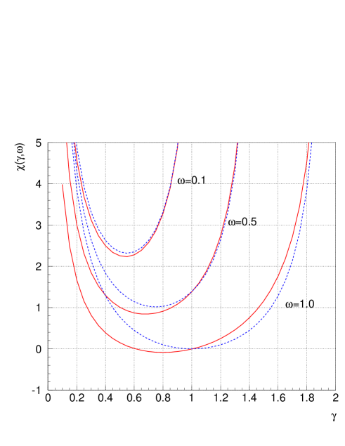
Figure 6: The eigenvalue of the BFKL kernel with the kinematical constraint of the form (6) dashed lines, and (8) solid lines. Calculation performed for three different values of the Mellin variable $\omega=0.1,0.5,1.0$.

5 Conclusions

The BFKL equation in the leading logarithmic approximation suffers from the problem of the violation of the energy - momentum conservation. The kinematical constraint reduces the phase space allowed for the the real emissions and is responsible for the resummation of the subleading corrections. The kernel eigenvalue in that case is zero when $\omega=1$ and $\gamma=1/2$. This means that in the limit $\bar{\alpha}_{s}\rightarrow\infty$ the intercept becomes equal to 1, which can be interpreted as an exchange of the color- singlet object with spin 2. When the momentum sum rule is additionally imposed, the effective eigenvalue becomes constant and equal to one in the limit of the infinite strong coupling. Such model then can provide an interpolation between the small and large values of the strong coupling constant. The first correction to the intercept of the graviton, of the form $1/\sqrt{\bar{\alpha}_{s}}$ can be also computed from this model. The more accurate form of the kinematical constraint further reduces the eigenvalue. However, the overall qualitative behavior remains unchaged and the model still has to be supplemented by the requirement that at $\omega=1$ the eigenvalue vanishes for all values of the Mellin variable $\gamma$.

This result is valid in the case of one Pomeron exchange. We stress that the result for the intercept will be renormalized when the multi-Pomeron exchanges or the saturation corrections are also incorporated. These corrections will certainly become important in the limit of the very large coupling. Also, the running of the coupling and the presence of quarks in the evolution can further change the results in a quantitative way. We leave these questions for further studies.

References

-
[1]
L.N. Lipatov, Sov. J. Nucl. Phys. 23 338 (1976);
E.A. Kuraev, L.N. Lipatov and V.S. Fadin, Sov. Phys. JETP 45 199 (1977);
I.I. Balitsky and L.N. Lipatov, Sov. J. Nucl. Phys. 28 338 (1978). -
[2]
V.S. Fadin, M.I. Kotsky and R. Fiore, Phys. Lett. B 359 181 (1995);
V.S. Fadin, M.I. Kotsky and L.N. Lipatov, BUDKERINP-96-92, hep-ph/9704267; V.S. Fadin, R. Fiore, A. Flachi and M.I. Kotsky, Phys. Lett. B 422 287 (1998);
V.S. Fadin and L.N. Lipatov, Phys. Lett. B 429 127 (1998).
- [3] G. Camici and M. Ciafaloni, Phys. Lett. B 386 341 (1996); Phys. Lett. B 412 396 (1997), [Erratum-ibid.Phys. Lett. B 417 390 (1997)]; Phys. Lett. B 430 349 (1998).
- [4] G. Altarelli, R. D. Ball and S. Forte, Nucl. Phys. B 575, 313 (2000).
- [5] G. Altarelli, R. D. Ball and S. Forte, Nucl. Phys. B 599, 383 (2001).
- [6] G. Altarelli, R. D. Ball and S. Forte, arXiv:hep-ph/0104246.
- [7] G. Altarelli, R. D. Ball and S. Forte, Nucl. Phys. B 621, 359 (2002).
- [8] G. Altarelli, R. D. Ball and S. Forte, Nucl. Phys. B 674, 459 (2003).
- [9] G. Altarelli, R. D. Ball and S. Forte, Nucl. Phys. B 742, 1 (2006).
- [10] M. Ciafaloni and D. Colferai, Phys. Lett. B 452, 372 (1999).
- [11] M. Ciafaloni, D. Colferai and G. P. Salam, JHEP 9910, 017 (1999).
- [12] M. Ciafaloni, D. Colferai and G. P. Salam, Phys. Rev. D 60, 114036 (1999).
- [13] M. Ciafaloni, D. Colferai, G. P. Salam and A. M. Staśto, Phys. Rev. D 68, 114003 (2003).
- [14] M. Ciafaloni, D. Colferai, D. Colferai, G. P. Salam and A. M. Staśto, Phys. Lett. B 576, 143 (2003).
- [15] M. Ciafaloni, D. Colferai, G. P. Salam and A. M. Staśto, Phys. Lett. B 587, 87 (2004).
- [16] R.S. Thorne, Phys. Rev. D 64 074005 (2001); Phys. Lett. B 474 372 (2000).
- [17] J. Kwieciński, A. D. Martin and A. M. Staśto, Phys. Rev. D 56, 3991 (1997).
- [18] A. V. Kotikov, L. N. Lipatov and V. N. Velizhanin, Phys. Lett. B 557, 114 (2003).
- [19] A. V. Kotikov, L. N. Lipatov, A. I. Onishchenko and V. N. Velizhanin, Phys. Lett. B 595, 521 (2004) [Erratum-ibid. B 632, 754 (2006)].
- [20] J. C. Collins, Acta Phys. Polon. B 34, 3103 (2003).
- [21] J. C. Collins and X. Zu, JHEP 0503, 059 (2005).
- [22] J.C. Collins, T. Rogers and A.M. Staśto, in preparation.
- [23] J. M. Maldacena, Adv. Theor. Math. Phys. 2, 231 (1998) [Int. J. Theor. Phys. 38, 1113 (1999)].
- [24] R. C. Brower, J. Polchinski, M. J. Strassler and C. I. Tan, arXiv:hep-th/0603115.
- [25] R. A. Janik, Phys. Lett. B 500, 118 (2001).
- [26] R. A. Janik and R. Peschanski, Nucl. Phys. B 565, 193 (2000).
- [27] B. Andersson, G. Gustafson, H. Kharraziha and J. Samuelsson, Z. Phys. C 71 613 (1996).
- [28] J. Kwieciński, A. D. Martin and P. J. Sutton, Z. Phys. C 71 585 (1996).
- [29] M. Ciafaloni, Nucl. Phys. B 296 49 (1988).
- [30] E. Avsar, G. Gustafson and L. Lonnblad, arXiv:hep-ph/0610157.
- [31] E. Avsar, G. Gustafson and L. Lonnblad, JHEP 0507, 062 (2005).
- [32] G.P. Salam, JHEP 9807 19 (1998).