Angular correlations of lepton pairs from vector boson and top quark decays in
Monte Carlo simulations

Abstract:

We explain how angular correlations in leptonic decays of vector bosons and top quarks can be included in Monte Carlo parton showers, in particular those matched to NLO QCD computations. We consider the production of $n$ pairs of leptons, originating from the decays of $n$ electroweak vector bosons or of $n$ top quarks, in the narrow-width approximation. In the latter case, the information on the $n$ $b$ quarks emerging from the decays is also retained. We give results of implementing this procedure in MC@NLO.

1 Introduction

Accurate predictions for the spectra of the leptons emerging from decays of vector bosons or top quarks are important for a variety of studies at hadron colliders, such as acceptance computations, tests of QCD, and searches for new physics. Theoretical computations should be based on all Feynman diagrams in which the corresponding leptons are external legs. In general, not all such diagrams are resonant diagrams, i.e. those in which the leptons directly emerge from a vector boson propagator (which, in the case of top decays, in turn is directly connected to the top quark via a $Wtb$ vertex). Usually, however, predictions based on computations that retain only the resonant diagrams are excellent approximations to those based on the fuller set of diagrams, owing to the rather narrow widths of the vector bosons and top quarks; the more so in the presence of final-state cuts which are designed to enhance on-shell contributions.

A further approximation can be made, which we call the decay chain approximation: resonant diagrams are replaced by diagrams relevant to the production of on-shell vector bosons or top quarks, times the diagrams corresponding to the matrix elements for the decays. In this way, off-shell effects are lost, but they can be recovered to some accuracy by reweighting the results of the decay chain approximation by a Breit-Wigner function. There is another piece of information that is lost in the decay chain approximation, and cannot be recovered, namely that on production angular correlations (more precisely, angular correlations due to production spin correlations). Let us denote by $P$ the decaying particle (a vector boson or a top in our case), and by $d_{1}$, $\ldots$, $d_{n}$ its decay products, and consider the hard process

$$a+b\;\longrightarrow\;P(\longrightarrow d_{1}+\cdots+d_{n})+X\,,$$ (1)

with $X$ a set of final-state particles which may also contain other decaying vector bosons or top quarks. The process of eq. (1) is said to have decay angular correlations if the matrix elements of the corresponding resonant Feynman diagrams have a non-trivial dependence on $(d_{i}\!\cdot\!d_{j})$. Clearly, decay correlations are always present if the particle $P$ has spin different from zero. The process of eq. (1) has production angular correlations if its matrix elements have a non-trivial dependence on $(d_{i}\!\cdot\!a)$, $(d_{i}\!\cdot\!b)$, or $(d_{i}\!\cdot\!X)$. It is therefore clear that the decay chain approximation can account for the decay correlations, but not for the production correlations.

The decay chain approximation has obvious advantages, leading to much simpler computations (especially at higher orders) owing to the reduced multiplicity of the final state. Still, it is not acceptable if the spectra of the decay products must be predicted with some accuracy. The aim of this paper is to introduce an approach to the computations of lepton spectra as given by resonant diagrams, which uses the decay chain approximation but also correctly accounts for production angular correlations. The method is primarily intended to be applied to parton shower Monte Carlos, including those that implement NLO QCD corrections such as MC@NLO [1, 2] or POWHEG [3]. The idea stems from the following observation: the matrix elements computed with the resonant diagrams are bounded from above by the matrix elements obtained by eliminating the decay products and putting the parent particles (vector bosons and/or top quarks) on-shell, times a process-independent constant. One can therefore use the latter matrix elements (which we call undecayed matrix elements) to perform computing-intensive tasks for which production correlations are not an issue. When the four-momenta of the parent particles are available, the resonant diagrams (we refer to the corresponding matrix elements as leptonic ones) are used in the context of a simple hit-and-miss procedure to generate the leptonic four-momenta.

In order to apply a hit-and-miss procedure, we need upper bounds on the decay matrix elements that are universal with respect to the production process. These are derived in the following section, first for vector boson, then for top quark decay, and finally for final states containing several vector bosons and/or top quarks. The practical application of these results is discussed in section 3. The inclusion of angular correlations in NLO computations is hampered by the presence of virtual corrections and the necessity for subtraction terms, which mean that one has to deal with expressions that are not simply matrix elements squared, and therefore are not necessarily positive-definite. This implies that the scheme we propose in this paper is such that angular correlations are not accurate to NLO in the whole phase space, but are correct to NLO for hard real emissions and to LO in soft and collinear regions. Obviously, one can implement angular correlations exactly to NLO accuracy by using lepton matrix elements in all the steps of the computation. In this paper, however, we are solely interested in the decay chain approximation. Illustrative results of our approach, obtained with MC@NLO, are presented in section 4, followed by our conclusions in section 5. An appendix presents an alternative derivation of the upper bound for vector boson decay, which may clarify some of the assumptions involved.

2 Upper bounds for the leptonic matrix elements

In this section, we derive the universal factors that, when multiplied by the undecayed matrix elements, give an upper bound for the leptonic matrix elements. After introducing some notation, we shall treat the cases of the vector bosons and of the top quarks in turn.

2.1 Notations

We shall always denote by

$$V\;\;\longrightarrow\;\;l\overline{l}$$ (2)

the decay of the vector boson $V\equiv W$ or $Z$ into a lepton-antilepton pair, which means that in the case of $W$ decay $\overline{l}$ is not the antiparticle of $l$. In our conventions, the $Vl\overline{l}$ vertex is

$$-iF_{V}\gamma^{\mu}\left(V_{Vl}-A_{Vl}\gamma_{5}\right)\,,$$ (3)

where

$$F_{Z}=\frac{g_{\scriptscriptstyle\rm W}}{2\cos\theta_{\scriptscriptstyle\rm W}},\;\;\;\;V_{Zl}=V_{l},\;\;\;\;A_{Zl}=A_{l};$$ (4)

$$F_{W}=\frac{g_{\scriptscriptstyle\rm W}}{2\sqrt{2}},\;\;\;\;V_{Wl}=1,\;\;\;\;A_{Wl}=1.$$ (5)

We shall consider the process

$$a(P_{1})+b(P_{2}) \longrightarrow V_{1}(q_{1})+\ldots+V_{n}(q_{n})+X(x)$$ (6)

$$\longrightarrow l_{1}(k_{1})+\overline{l}_{1}(k_{2})+\ldots+l_{n}(k_{2n-1})+\overline{l}_{n}(k_{2n})+X(x),$$ (7)

where

$$q_{i}=k_{2i-1}+k_{2i}\,,$$ (8)

and $X$ collectively denotes any particles not originating from a vector boson decay. It is particularly convenient to write the phase space of the final-state particles of eq. (7) as follows

$$d\Phi_{2n+1^{\!\star}}(P_{1}+P_{2};k_{1},\ldots,k_{2n},x)=$$

$$\phantom{d\Phi a}d\Phi_{n+1^{\!\star}}(P_{1}+P_{2};q_{1},\ldots,q_{n},x)\,\prod_{i=1}^{n}d\Phi_{2}(q_{i};k_{2i-1},k_{2i})\,\frac{dq_{i}^{2}}{2\pi}\,.$$ (9)

As the notation $1^{\!\star}$ suggests, we treat the particles $X$ as a single particle with mass-squared $x^{2}$ and four-momentum $x$, since the individual four-momenta of the particles $X$ are irrelevant in what follows. On the r.h.s. of eq. (9), the two-body phase spaces account for the decays

$$V_{i}(q_{i})\;\longrightarrow\;l_{i}(k_{2i-1})+\overline{l}_{i}(k_{2i}).$$ (10)

The factorization formula of eq. (9) is exact: the vector bosons are off-shell, and their virtualities $q_{i}^{2}$ (i.e., the invariant masses of the lepton pairs) are explicitly integrated over. This decomposition has an obvious physical interpretation in the context of resonant diagrams.

In the case of processes involving top quarks, we shall deal with

$$a(P_{1})+b(P_{2}) \longrightarrow t_{1}(p_{1})+\ldots+t_{n}(p_{n})+X(x)$$ (11)

$$\longrightarrow W_{1}(q_{1})+b_{1}(r_{1})+\ldots+W_{n}(q_{n})+b_{n}(r_{n})+X(x)$$ (13)

$$\longrightarrow l_{1}(k_{1})+\nu_{1}(k_{2})+b_{1}(r_{1})+\ldots+l_{n}(k_{2n-1})+\nu_{n}(k_{2n})+b_{n}(r_{n})$$

$$+X(x)\,,$$

where $t$ can be either a top or an antitop. As in eq. (9), we can also write the exact phase-space factorization

$$d\Phi_{3n+1^{\!\star}}(P_{1}+P_{2};k_{1},\ldots,k_{2n},r_{1},\ldots,r_{n},x)=$$

$$\phantom{d\Phi a}d\Phi_{n+1^{\!\star}}(P_{1}+P_{2};p_{1},\ldots,p_{n},x)\,\prod_{i=1}^{n}d\Phi_{3}(p_{i};k_{2i-1},k_{2i},r_{i})\,\frac{dp_{i}^{2}}{2\pi}\,,$$ (14)

with the three-body phase spaces on the r.h.s. accounting for the decays

$$t_{i}(p_{i})\;\longrightarrow\;W_{i}(q_{i})+b_{i}(r_{i})\;\longrightarrow\;l_{i}(k_{2i-1})+\nu_{i}(k_{2i})+b_{i}(r_{i}).$$ (15)

2.2 Vector boson decay

We start by considering the production of one $l\overline{l}$ pair, and we neglect the $Z/\gamma$ interference. The amplitude for the process in eq. (7) with $n=1$ is

$$A=M^{\mu}\frac{i}{q^{2}-m_{V}^{2}+im_{V}\Gamma_{V}}\left(-g_{\mu\nu}+\frac{q_{\mu}q_{\nu}}{m_{V}^{2}}\right)\overline{u}(k_{1})(-iF_{V})\gamma^{\nu}\left(V_{Vl}-A_{Vl}\gamma_{5}\right)v(k_{2})\,,$$ (16)

where $m_{V}$ and $\Gamma_{V}$ are the mass and the width of the vector boson respectively, and $M^{\mu}$ is the amplitude for the process

$$a(P_{1})+b(P_{2})\,\longrightarrow\,V(q)+X(x)\,,$$ (17)

$\mu$ being the Lorentz index associated with $V$; the polarization four-vector of $V$ is not included in $M^{\mu}$. From eq. (16) we get (neglecting lepton masses)

$$\sum_{\rm spins}\left|A\right|^{2} = M^{\mu}M^{*\rho}\frac{\left(-g_{\mu\nu}+q_{\mu}q_{\nu}/m_{V}^{2}\right)\left(-g_{\rho\sigma}+q_{\rho}q_{\sigma}/m_{V}^{2}\right)}{(q^{2}-m_{V}^{2})^{2}+(m_{V}\Gamma_{V})^{2}}$$ (18)

$$\times F_{V}^{2}\,{\rm Tr}\!\left[\left(V_{Vl}^{2}+A_{Vl}^{2}-2V_{Vl}A_{Vl}\gamma_{5}\right)/\!\!\!k_{1}\gamma^{\nu}/\!\!\!k_{2}\gamma^{\sigma}\right].$$

We now consider the narrow width approximation $\Gamma_{V}\to 0$. We have

$$\frac{1}{(q^{2}-m_{V}^{2})^{2}+(m_{V}\Gamma_{V})^{2}}\;\longrightarrow\;\frac{\pi}{m_{V}\Gamma_{V}}\,\delta\left(q^{2}-m_{V}^{2}\right)\,.$$ (19)

The $\delta$ function, which puts the vector boson on shell, allows us to write

$$\left(-g^{\mu\nu}+\frac{q^{\mu}q^{\nu}}{m_{V}^{2}}\right)=\sum_{\lambda}\varepsilon_{\lambda}^{\mu}\varepsilon_{\lambda}^{*\nu},$$ (20)

where $\varepsilon_{\lambda}$ are the polarization four-vectors of the vector boson. Using eq. (20), eq. (18) becomes

$$\sum_{spin}\left|A\right|^{2}=\frac{\pi}{m_{V}\Gamma_{V}}\sum_{\lambda\lambda^{\prime}}\tilde{M}_{\lambda}\rho_{\lambda\lambda^{\prime}}\tilde{M}^{*}_{\lambda^{\prime}}\,\delta\left(q^{2}-m_{V}^{2}\right),$$ (21)

where we defined

$$\tilde{M}_{\lambda}=M_{\mu}\varepsilon_{\lambda}^{\mu}\,,$$ (22)

which is the amplitude for the process of eq. (17) for a given vector boson polarization $\lambda$. We also define

$$\rho_{\lambda\lambda^{\prime}}=F_{V}^{2}\,{\rm Tr}\!\left[\left(V_{Vl}^{2}+A_{Vl}^{2}-2V_{Vl}A_{Vl}\gamma_{5}\right)/\!\!\!k_{1}/\!\!\!\varepsilon_{\lambda}^{*}/\!\!\!k_{2}/\!\!\!\varepsilon_{\lambda^{\prime}}\right]$$ (23)

which is, apart from the normalization, the decay density matrix of the vector boson. This quantity can be explicitly computed; here, we only present it in the form of a diagonal matrix

$$\rho_{\lambda\lambda^{\prime}}=\left(U\rho^{D}U^{*}\right)_{\lambda\lambda^{\prime}}\,,$$ (24)

where

$$\rho^{D}=2m_{V}^{2}F_{V}^{2}\,{\rm diag}\left(0,(V_{Vl}-A_{Vl})^{2},(V_{Vl}+A_{Vl})^{2}\right).$$ (25)

The cross section for the production of a lepton pair in the narrow width approximation is therefore

$$d\sigma_{l\overline{l}} = \frac{1}{2s}\frac{\pi}{m_{V}\Gamma_{V}}\sum_{\lambda\lambda^{\prime}}\left(\tilde{M}U\right)_{\lambda}\rho_{\lambda\lambda^{\prime}}^{D}\left(\tilde{M}U\right)^{*}_{\lambda^{\prime}}\,\delta\left(q^{2}-m_{V}^{2}\right)$$ (26)

$$\times\frac{dq^{2}}{2\pi}\,d\Phi_{1+1^{\!\star}}(P_{1}+P_{2};q,x)\,d\Phi_{2}(q;k_{1},k_{2})\,.$$

Owing to the hermiticity properties of the density matrices, and to the explicit form of eq. (25), eq. (26) is a positive-definite quadratic form in the space of the spin indices of the vector boson. Thus

$$d\sigma_{l\overline{l}}\leq\frac{1}{2s}\frac{\pi}{m_{V}\Gamma_{V}}\max_{\lambda}\left(\rho_{\lambda\lambda}^{D}\right)|\tilde{M}|^{2}\frac{1}{2\pi}\,d\Phi_{1+1^{\!\star}}\,d\Phi_{2}\,,$$ (27)

where

$$|\tilde{M}|^{2}=\sum_{\lambda}\tilde{M}_{\lambda}\tilde{M}^{*}_{\lambda}=\sum_{\lambda}\left(\tilde{M}U\right)_{\lambda}\left(\tilde{M}U\right)^{*}_{\lambda}=M^{\mu}M^{*\nu}\left(-g_{\mu\nu}+\frac{q_{\mu}q_{\nu}}{m_{V}^{2}}\right)\,,$$ (28)

with $q^{2}=m_{V}^{2}$. Eq. (27) cannot be used as an upper bound for the matrix element of the process (7), since the measures on the two sides are different. Using eq. (19), we can however easily reinstate the $q^{2}$ integration by inserting

$$1=\int\!dq^{2}\,\frac{m_{V}\Gamma_{V}}{\pi}\,\frac{1}{(q^{2}-m_{V}^{2})^{2}+(m_{V}\Gamma_{V})^{2}}$$ (29)

on the r.h.s. of eq. (27). Furthermore, from eq. (25) we obtain:

$$\max_{\lambda}\left(\rho_{\lambda\lambda}^{D}\right)=2m_{V}^{2}F_{V}^{2}\,(V_{Vl}+A_{Vl})^{2}\,,$$ (30)

which holds since $V_{Vl}A_{Vl}>0$ regardless of the identity of the lepton $l$. Therefore

$$\frac{1}{2s}\sum_{spin}\left|A\right|^{2}\equiv\frac{d\sigma_{l\overline{l}}}{d\Phi_{2+1^{\!\star}}}\leq\frac{2m_{V}^{2}\,F_{V}^{2}\,(V_{Vl}+A_{Vl})^{2}}{(q^{2}-m_{V}^{2})^{2}+(m_{V}\Gamma_{V})^{2}}\,\frac{|\tilde{M}|^{2}}{2s}\,,$$ (31)

which strictly speaking holds only when $q^{2}=m_{V}^{2}$, since all results in this section are formally derived in the limit $\Gamma_{V}\to 0$. More details on this, and the reason for keeping a formal dependence on $q^{2}$ in eq. (31), will be given in appendix A. Eq. (31) is the main result of this section. It states that, in the narrow width approximation, the lepton-pair cross section has an upper bound, which is a universal factor times the cross section for the production of the parent vector boson

$$\frac{d\sigma_{V}}{d\Phi_{1+1^{\!\star}}}=\frac{1}{2s}\,|\tilde{M}|^{2}\,.$$ (32)

2.3 Top decay

Here, we consider the decay of a top quark

$$t(p)\;\longrightarrow\;W^{+}(q)+b(r)\;\longrightarrow\;l^{+}(k_{1})+\nu(k_{2})+b(r);$$ (33)

the treatment of the decay of an antitop is fully analogous. Other top quarks may be present in the final state, but their decays are of no interest for the moment, and will be ignored. The amplitude for the process in eq. (13) is

$$A = \overline{u}(r)V_{tb}\frac{g_{\scriptscriptstyle\rm W}}{2\sqrt{2}}\gamma^{\mu}(1-\gamma_{5})\frac{/\!\!\!p+m_{t}}{p^{2}-m_{t}^{2}+im_{t}\Gamma_{t}}M$$ (34)

$$\times \frac{-g_{\mu\nu}+q_{\mu}q_{\nu}/m_{W}^{2}}{q^{2}-m_{W}^{2}+im_{W}\Gamma_{W}}\overline{u}(k_{2})\frac{g_{\scriptscriptstyle\rm W}}{2\sqrt{2}}\gamma^{\nu}(1-\gamma_{5})v(k_{1})\,,$$

where $M$ is the amplitude for the process

$$a(P_{1})+b(P_{2})\,\longrightarrow\,t(p)+X(x)\,,$$ (35)

except for a spinor $\overline{u}(p)$, which is not included. Therefore, $M=\Gamma u(K)$, with $\Gamma$ a combination of $\gamma$ matrices, and $K$ the four-momentum of a fermion entering the hard scattering. By squaring eq. (34) we get

$$\left|A\right|^{2} = \frac{g_{\scriptscriptstyle\rm W}^{4}\left|V_{tb}\right|^{2}}{64}\frac{1}{(p^{2}-m_{t}^{2})^{2}+(m_{t}\Gamma_{t})^{2}}\frac{1}{(q^{2}-m_{W}^{2})^{2}+(m_{W}\Gamma_{W})^{2}}$$ (36)

$$\times \overline{u}(r)\gamma^{\mu}(1-\gamma_{5})\left(/\!\!\!p+m_{t}\right)MM^{*}\gamma^{0}\left(/\!\!\!p+m_{t}\right)(1+\gamma_{5})\gamma^{\rho}u(r)$$

$$\times \overline{u}(k_{2})\gamma_{\mu}(1-\gamma_{5})v(k_{1})\overline{v}(k_{1})(1+\gamma_{5})\gamma_{\rho}u(k_{2})\,.$$

Following what was done in eq. (18), we now consider eq. (36) in the narrow width approximation $\Gamma_{t}\to 0$, i.e. we make the replacement

$$\frac{1}{(p^{2}-m_{t}^{2})^{2}+(m_{t}\Gamma_{t})^{2}}\;\longrightarrow\;\frac{\pi}{m_{t}\Gamma_{t}}\,\delta\left(p^{2}-m_{t}^{2}\right)\,.$$ (37)

Thanks to the on-shell condition introduced in this way, we can use the analogue of eq. (20)

$$/\!\!\!p+m_{t}=\sum_{\lambda}u_{\lambda}(p)\overline{u}_{\lambda}(p),$$ (38)

which in turn suggests introducing the quantity

$$\tilde{M}_{\lambda}=\overline{u}_{\lambda}(p)M\;\;\;\Longrightarrow\;\;\;\tilde{M}_{\lambda}^{*}=M^{*}\gamma^{0}u_{\lambda}(p),$$ (39)

which is the analogue of eq. (22), and is the amplitude for the process of eq. (35) for a given top polarization $\lambda$. Upon summing over the spins of the final-state leptons and $b$ quark, eq. (36) can be cast in the same form as eq. (21):

$$\sum_{spin}\left|A\right|^{2}=\frac{\pi}{m_{t}\Gamma_{t}}\sum_{\lambda\lambda^{\prime}}\tilde{M}_{\lambda}\rho_{\lambda\lambda^{\prime}}\tilde{M}^{*}_{\lambda^{\prime}}\,\delta\left(p^{2}-m_{t}^{2}\right),$$ (40)

with

$$\rho_{\lambda\lambda^{\prime}} = \frac{g_{\scriptscriptstyle\rm W}^{4}\left|V_{tb}\right|^{2}}{16}\frac{1}{(q^{2}-m_{W}^{2})^{2}+(m_{W}\Gamma_{W})^{2}}\,\,{\rm Tr}\!\left[(1-\gamma_{5})/\!\!\!k_{2}\gamma_{\mu}/\!\!\!k_{1}\gamma_{\rho}\right]$$ (41)

$$\times \overline{u}_{\lambda^{\prime}}(p)(1+\gamma_{5})\gamma^{\rho}/\!\!\!r\gamma^{\mu}u_{\lambda}(p)\,.$$

This is the decay density matrix for the top quark, the analogue of eq. (23). We can now proceed exactly as was done in sect. 2.2, and therefore we must compute the decay density matrix, diagonalize it, and find the largest of the matrix elements so obtained. An explicit computation leads to

$$\rho^{D}=\frac{4g_{\scriptscriptstyle\rm W}^{4}\left|V_{tb}\right|^{2}}{(q^{2}-m_{W}^{2})^{2}+(m_{W}\Gamma_{W})^{2}}\,(r\!\cdot\!k_{2})(p\!\cdot\!k_{1})\,{\rm diag}(0,1)\,.$$ (42)

Using eq. (42) and reinstating the integral in $dp^{2}$ using the analogue of eq. (29), we finally arrive at

$$\frac{1}{2s}\sum_{spin}\left|A\right|^{2}\equiv\frac{d\sigma_{l\nu b}}{d\Phi_{3+1^{\!\star}}}\leq\frac{4g_{\scriptscriptstyle\rm W}^{4}\left|V_{tb}\right|^{2}(r\!\cdot\!k_{2})(p\!\cdot\!k_{1})}{\Big{(}(q^{2}-m_{W}^{2})^{2}+(m_{W}\Gamma_{W})^{2}\Big{)}\Big{(}(p^{2}-m_{t}^{2})^{2}+(m_{t}\Gamma_{t})^{2}\Big{)}}\,\frac{|\tilde{M}|^{2}}{2s}\,,$$ (43)

which strictly speaking holds only when $p^{2}=m_{t}^{2}$. Eq. (43) is the analogue of eq. (31), and expresses the upper bound on the matrix elements for the production of $l\nu b$ in terms of the matrix elements for the production of a top quark

$$\frac{d\sigma_{t}}{d\Phi_{1+1^{\!\star}}}=\frac{1}{2s}\,|\tilde{M}|^{2}\,.$$ (44)

In contrast to eq. (31), the bound of eq. (43) is not a constant over the phase space of the particles emerging from top decay, because of its dependence on $(r\!\cdot\!k_{2})$ and $(p\!\cdot\!k_{1})$. This helps to increase the efficiency of event generation in the context of an unweighting procedure, but in order to avoid any biases the phase-space must be sampled in such a way as to reproduce exactly the $q^{2}$-, $(r\!\cdot\!k_{2})$-, and $(p\!\cdot\!k_{1})$-dependences of the bound. An alternative approach is that of finding a constant larger than or equal to the bound, which can be done by finding the maximum of the combination of dot products

$$D=(r\!\cdot\!k_{2})(p\!\cdot\!k_{1})\,.$$ (45)

Using the top rest frame to perform the relevant computations, it is a matter of simple algebra to obtain

$$D\leq D_{\max}(q^{2})=\left\{\begin{array}[]{ll}m_{t}^{4}/16&\phantom{aaaa}q^{2}\leq\frac{m_{t}^{2}}{2}\,,\\ q^{2}(m_{t}^{2}-q^{2})/4&\phantom{aaaa}\frac{m_{t}^{2}}{2}<q^{2}\leq m_{t}^{2}\,.\end{array}\right.$$ (46)

Note that $m_{t}^{4}/16\geq q^{2}(m_{t}^{2}-q^{2})/4$ in the whole $q^{2}$ range, and therefore one can always set $D_{\max}=m_{t}^{4}/16$; this is seen to lead to a very marginal degradation of unweighting efficiency. We have therefore

$$\frac{d\sigma_{l\nu b}}{d\Phi_{3+1^{\!\star}}}\leq\frac{4g_{\scriptscriptstyle\rm W}^{4}\left|V_{tb}\right|^{2}D_{\max}(q^{2})}{\Big{(}(q^{2}-m_{W}^{2})^{2}+(m_{W}\Gamma_{W})^{2}\Big{)}\Big{(}(p^{2}-m_{t}^{2})^{2}+(m_{t}\Gamma_{t})^{2}\Big{)}}\,\frac{d\sigma_{t}}{d\Phi_{1+1^{\!\star}}}\,.$$ (47)

2.4 Multiple decays

It is easy to generalize the formulae derived in the previous sections to the cases in which one is interested in the decay products of several vector bosons and/or top quarks. Consider for example the process of eq. (7). An equation identical to eq. (16) holds, with the formal replacements

$$M^{\mu} \longrightarrow M^{\mu_{1}\ldots\mu_{n}}\,,$$ (48)

$$\frac{-g_{\mu\nu}+q_{\mu}q_{\nu}/m_{V}^{2}}{q^{2}-m_{V}^{2}+im_{V}\Gamma_{V}} \longrightarrow \prod_{i=1}^{n}\frac{-g_{\mu\nu}+q_{i\mu}q_{i\nu}/m_{V_{i}}^{2}}{q_{i}^{2}-m_{V_{i}}^{2}+im_{V_{i}}\Gamma_{V_{i}}}\,,$$ (49)

$$F_{V}\overline{u}(k_{1})\gamma^{\nu}\left(V_{Vl}-A_{Vl}\gamma_{5}\right)v(k_{2}) \longrightarrow \prod_{i=1}^{n}F_{V_{i}}\overline{u}(k_{2i-1})\gamma^{\nu}\left(V_{V_{i}l_{i}}-A_{V_{i}l_{i}}\gamma_{5}\right)v(k_{2i})\,.\phantom{aaa}$$ (50)

The analogue of eq. (26) features the quantity

$$\sum_{\lambda_{1}\lambda_{1}^{\prime}}\ldots\sum_{\lambda_{n}\lambda_{n}^{\prime}}\left(\tilde{M}U_{1}\ldots U_{n}\right)_{\lambda_{1}\ldots\lambda_{n}}\rho_{1\lambda_{1}\lambda_{1}^{\prime}}^{D}\ldots\rho_{n\lambda_{n}\lambda_{n}^{\prime}}^{D}\left(\tilde{M}U_{1}\ldots U_{n}\right)^{*}_{\lambda_{1}^{\prime}\ldots\lambda_{n}^{\prime}}\,,$$ (51)

which results from the simultaneous diagonalization of the spin density matrices of the $n$ vector bosons. This allows one to use eq. (30), and to proceed as in the previous section. We therefore arrive at

$$\frac{d\sigma_{l_{1}\overline{l}_{1}\ldots l_{n}\overline{l}_{n}}}{d\Phi_{2n+1^{\star}}}\leq\left(\prod_{i=1}^{n}\frac{2m_{V_{i}}^{2}\,F_{V_{i}}^{2}\,(V_{V_{i}l_{i}}+A_{V_{i}l_{i}})^{2}}{(q_{i}^{2}-m_{V_{i}}^{2})^{2}+(m_{V_{i}}\Gamma_{V_{i}})^{2}}\right)\,\frac{d\sigma_{V_{1}\ldots V_{n}}}{d\Phi_{n+1^{\star}}}\,,$$ (52)

where $d\sigma_{V_{1}\ldots V_{n}}$ is the cross section for the process of eq. (6), all the vector bosons being on-shell.

Along the same lines, eq. (47) can immediately be generalized to the case of the decays of several top and antitop quarks:

$$\frac{d\sigma_{l_{1}\nu_{1}b_{1}\ldots l_{n}\nu_{n}b_{n}}}{d\Phi_{3n+1^{\star}}}\leq$$

$$\phantom{aaaa}\left(\prod_{i=1}^{n}\frac{4g_{\scriptscriptstyle\rm W}^{4}\left|V_{tb}\right|^{2}D_{\max}(q_{i}^{2})}{\Big{(}(q_{i}^{2}-m_{W}^{2})^{2}+(m_{W}\Gamma_{W})^{2}\Big{)}\Big{(}(p_{i}^{2}-m_{t}^{2})^{2}+(m_{t}\Gamma_{t})^{2}\Big{)}}\right)\,\frac{d\sigma_{t_{1}\ldots t_{n}}}{d\Phi_{n+1^{\star}}}\,.\phantom{aaaa}$$ (53)

Obviously, eqs. (52) and (53) can be combined for the simultaneous presence of vector bosons and top quarks in the final state.

3 Angular correlations in MC@NLO

As mentioned in the introduction, the straightforward way to predict correctly all features of lepton spectra is to include in the computation the leptonic matrix elements, for example as done in MC@NLO version 3.3 [5] for the cases of single-$V$ or $V\!H$ production, or in refs. [6, 7] for the case of top quark decay in parton-level pure NLO computations. We remind the reader that, in the context of MC@NLO, parton-level cross sections (which are obtained by suitably modifying those which enter pure-NLO computations) are first integrated over the phase space of the final-state particles. The information gathered in this integration step is then used in the event-generation step, whose aim is that of obtaining a set of kinematic configurations (the hard events), which are subsequently showered by the parton shower Monte Carlo. We also point out that the same integration-and-generation structure is used by POWHEG (although the cross sections integrated in the two formalisms are not the same). The integration time increases rapidly with the number of final-state particles; there is a corresponding decrease in the efficiency of the generation of hard events. This is the reason why it is interesting to find alternative ways to predict angular correlations in large-multiplicity processes. We stress that in principle, the implementation in MC@NLO (or POWHEG) of a process with correct angular correlations is identical to that of the same process without such correlations. The problem is a practical one, namely that production angular correlations require the knowledge of the lepton matrix elements, and the increased multiplicity with respect to the undecayed matrix elements entails loss of accuracy and generation efficiency.

The strategy we propose in this paper starts with the following steps.

• Integrate the undecayed matrix elements.

• Generate hard events using the results of the previous step; thus, vectors bosons and/or top quarks will be present in the final state, but not their decay products.

• For each hard event, generate (massless) lepton (and $b$ quark, in the case of top decays) four-momenta, uniformly within the decay phase space(s) of the corresponding parent particle(s).

• Compute the lepton matrix element using the four-momenta obtained in step 3, and the undecayed matrix element using the four-momenta obtained in step 2. Generate a flat random number $r$. If the lepton matrix element, divided by its upper bound as given in eqs. (52) and (53), is smaller than $r$, throw the lepton four-momenta away, and return to step 3.

• Otherwise, replace the vector bosons and top quarks by the set of their decay products. The resulting kinematic configuration is the leptonic hard event that can be showered by the Monte Carlo.

Steps 3 to 5 constitute a standard hit-and-miss procedure, which guarantees that the lepton spectra reconstructed with the four-momenta of the leptonic hard event (and subsequent shower) will be identical to those computed by a direct integration of the leptonic matrix elements.

It is clear that the integration step will be greatly simplified by this procedure: the number of phase-space variables relevant to the undecayed processes (6) and (11) is $n_{U}=3(n+n_{X})-4$, whereas $n_{V}=3(2n+n_{X})-4$ and $n_{t}=3(3n+n_{X})-4$ for leptonic processes (7) and (13) respectively. On the other hand, one may doubt that the efficiency for producing leptonic hard events is larger than in the case of a straightforward integration of the leptonic matrix elements. In fact, the adaptive integration performed in step 1 will only give information on the $n_{U}$ degrees of freedom of the undecayed processes. However, using the phase-space decompositions of eqs. (9) and (14), one associates the extra $n_{V}-n_{U}=3n$ and $n_{t}-n_{U}=6n$ degrees of freedom with the decay phase spaces. Since we are considering here only resonant diagrams, the leptonic matrix elements will be fairly smooth in these extra $3n$ and $6n$ degrees of freedom, if the parametrizations of the decay phase spaces are properly chosen (the obvious choice of using the rest frame of the decaying particles is also an optimal choice from this point of view). Therefore, all of the complications due to the presence of several peaks in the matrix elements are dealt with in step 2. The unweighting performed in step 4 does not require any sophisticated numerical approach (i.e., a preliminary adaptive integration is not necessary) in order to achieve a satisfactory efficiency.

For the procedure as outlined above to work, it is crucial that the leptonic matrix elements can be bounded from above by the undecayed matrix elements. In the derivations of sect. 2 we have assumed that the density matrix is positive definite, which is the case, and that the matrix elements involved can be expressed as the modulus squared of an amplitude. This is certainly the case in the context of a tree-level computation, but it is not true for all the contributions to an NLO cross section. In particular, the interference between virtual and Born amplitudes is not positive-definite in general. The modified subtraction procedure [1] introduced in the MC@NLO formalism also implies the presence of a second quantity which is possibly not positive-definite, namely the difference between the real matrix elements and the MC subtraction terms. The presence of non-positive-definite contributions is what prevents one from including angular correlations exactly to NLO accuracy in the context of the decay chain approximation, as anticipated in sect. 1.

Before proceeding, we remind the reader that there are two classes of MC@NLO hard events, defined according to their kinematics: ${\mathbb{S}}$ (${\mathbb{H}}$) events have the same number of initial- and final-state particles as Born (real-emission) contributions. Thus, the number of final-state particles of ${\mathbb{H}}$ events is equal to that of ${\mathbb{S}}$ events, plus one. For example, in $W^{+}W^{-}$ production (eq. (6)) we have $(n,n_{X})=(2,0)$ for ${\mathbb{S}}$ events, and $(n,n_{X})=(2,1)$ for ${\mathbb{H}}$ events. In $t\bar{t}$ and single-top production (eq. (11)), we have $(n,n_{X})=(2,0)$ and $(n,n_{X})=(1,1)$ for ${\mathbb{S}}$ events, and $(n,n_{X})=(2,1)$ and $(n,n_{X})=(1,2)$ for ${\mathbb{H}}$ events respectively. POWHEG (and, for that matter, any NLO computation) also outputs ${\mathbb{S}}$ and ${\mathbb{H}}$ events.

We now extend the procedure proposed in points 1 to 5 above to the case of NLO computations matched to parton shower simulations, as follows:

• Steps 1 and 2 are unchanged.

• For each ${\mathbb{S}}$ event, go through steps 3 to 5, using Born-level results to compute lepton matrix elements and their upper bounds.

• For each ${\mathbb{H}}$ event, compute a quantity ${\cal G}({\mathbb{H}})$ as explained below and generate a random number $r^{\prime}$. If $r^{\prime}\!\leq{\cal G}({\mathbb{H}})$, go through steps 3 to 5, using real-emission results to compute lepton matrix elements and their upper bounds. If $r^{\prime}\!>{\cal G}({\mathbb{H}})$, define an ${\mathbb{S}}$-type event with the projection ${\cal P}_{{\mathbb{H}}\to{\mathbb{S}}}({\mathbb{H}})$, and proceed as explained for ${\mathbb{S}}$ events above.

The definition of a map ${\cal P}_{{\mathbb{H}}\to{\mathbb{S}}}$ is a necessary condition for the matching between NLO results and parton shower simulations: for more details see e.g. refs. [2, 8]. This implies that such a map need not be defined specifically for the purpose of including angular correlations into MC@NLO or POWHEG. The quantity ${\cal G}$ is a largely arbitrary smooth and continuous function, that assumes values between 0 and 1, and tends to 0 (1) in the soft/collinear (hard-emission) regions. The role of ${\cal G}$ is simply to avoid computing real-emission matrix elements in the phase-space regions where they diverge. In the context of MC@NLO, functions with the same behaviour as ${\cal G}$ need be introduced in order to ensure local cancellation between real matrix elements and MC counterterms (see e.g. app. A.5 of ref. [1] and app. B of ref. [2]), and one obvious choice is that of setting ${\cal G}$ equal to one of these functions (or to a combination of them).

It should be clear that the proposal made here accounts for angular correlations to LO accuracy close to the soft and collinear regions, since there ${\cal G}({\mathbb{H}})\simeq 0$, and therefore ${\mathbb{H}}$ events are projected onto ${\mathbb{S}}$ events, for which we only consider the Born matrix elements in the hit-and-miss procedure. On the other hand, in the hard emission region only real corrections contribute to the cross section, and thus angular correlations are included exactly to NLO accuracy. Angular correlations resulting from an MC matched to an NLO computation and implementing the method proposed in this paper have therefore the same or a better accuracy than LO-based Monte Carlos. We also stress that angular correlations are actually fairly close to those computed exactly to NLO, for two reasons. First, NLO corrections to spin correlations are generally small. Second, although virtual corrections and subtracted terms are not positive definite, their angular correlations arising from the contributions (if any) that are proportional to the Born matrix elements can be included exactly in the computation following the method proposed here, since both sides of eqs. (52) and (53) then get multiplied by the same factor.

4 Results

The approach described in the previous section has been adopted to include production angular correlations in MC@NLO in the cases of $W^{+}W^{-}$ production (since version 3.1) and of $t\bar{t}$ and single-$t$ production (since version 3.3). In this section we present sample results for $t\bar{t}$ and single-$t$ production, at the LHC ($pp$ collisions at $\sqrt{S}=14$ TeV) and at the Tevatron run II ($p\bar{p}$ collisions at $\sqrt{S}=1.96$ TeV). All the predictions given in this section have been obtained by using the MRST2002 default PDF set [9], and by setting $m_{t}=175$ GeV and $\Gamma_{t}=1.7$ GeV. In the case of single-$t$ production, we also reconstruct the accompanying jets, by means of the $k_{\scriptscriptstyle\rm T}$-clustering algorithm [10], with $d_{cut}=100$ GeV². We include in the clustering procedure all final-state stable hadrons and photons. For the sake of simplicity, we force $\pi^{0}$’s and all lowest-lying $b$-flavoured states to be stable in HERWIG. The jets are ordered in transverse momentum.

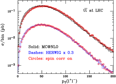
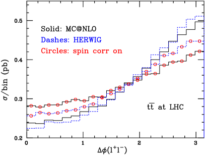
Figure 1: Transverse momentum of the lepton pair (left pane), and difference in azimuthal angle between the leptons (right pane), in $t\bar{t}$ production at the LHC. HERWIG results have been rescaled (by 0.3 on the left, and by the factor $K=\sigma_{\scriptscriptstyle\rm NLO}/\sigma_{\scriptscriptstyle\rm LO}$ on the right).

We begin by considering $t\bar{t}$ production. We have studied, at the Tevatron and at the LHC, single-inclusive $p_{\scriptscriptstyle\rm T}$ and rapidity spectra of the $t$ and $\bar{t}$ decay products, and the correlations in transverse momentum, $\Delta\phi$, and invariant mass of the $b\bar{b}$, $l^{+}l^{-}$, $bl^{-}$, $\bar{b}l^{+}$, $b\bar{\nu}$, and $\bar{b}\nu$ pairs. We have found that angular correlations have an almost negligible impact. We present in fig. 1 the only two observables for which these correlations have a visible effect, albeit barely so for $p_{\scriptscriptstyle\rm T}(l^{+}l^{-})$. On the other hand, angular correlations are an important ingredient for the correct prediction of $\Delta\phi(l^{+}l^{-})$, as shown in the right pane of fig. 1. It is interesting that about 30% of the difference between the LO prediction without angular correlations (dashed histogram – HERWIG) and the NLO prediction with angular correlations (solid histogram, overlayed with open circles – MC@NLO) is due to beyond-LO corrections.

It is possible to specifically design observables which would be trivial if angular correlations were neglected. Typically, such observables are angular variables constructed with the decay products of the top quarks, and measured in the rest frames of the parent particle. We have considered the distributions in $\cos\theta_{1}$, $\cos\theta_{2}$, and $\cos\phi$, as defined in ref. [11]; in particular, $\phi$ is the angle between the direction of flight of $l^{+}$ and the direction of flight of $l^{-}$. The directions of flight are defined in the $t$ and $\bar{t}$ rest frames respectively (see ref. [11] for more details). Results for $\cos\phi$ are presented in fig. 2 for the Tevatron (left pane) and the LHC (right pane). Just as for $\Delta\phi(l^{+}l^{-})$, beyond-LO contributions are not negligible, and they tend to deplete (at the Tevatron) or to enhance (at the LHC) the LO predictions for the $\cos\phi$ asymmetry. This behaviour is also found in the pure-NLO, parton-level study of ref. [11]. We have verified that, by neglecting angular correlations, the cross section depends trivially on $\theta_{1}$, $\theta_{2}$ and $\phi$.

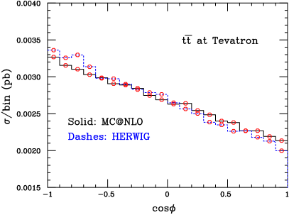
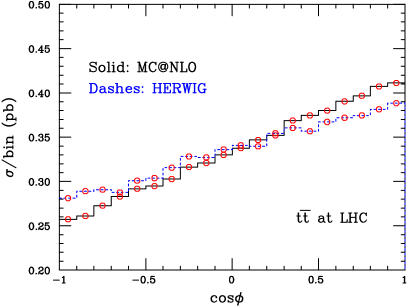
Figure 2: Opening angle distributions, as defined in the text, for $t\bar{t}$ production at the Tevatron (left pane) and at the LHC (right pane). HERWIG results have been rescaled by the $K$ factor. The corresponding curves obtained by neglecting angular correlations are flat, and are not shown in the figure.

Finally, we examine distributions for single-top production at the Tevatron. Because both production and decay occur through the left-handed charged current interaction, one expects stronger production angular correlations than in top quark pair production. Indeed, angular correlation effects are clearly visible in the single-inclusive spectra of the top decay products. As in the case of $t\bar{t}$ production, it is possible to study angular correlations more directly by choosing specific observables. These observables always involve the definition of a spin basis that leads to nearly 100% correlation between the direction of the charged lepton from top decay and another experimentally-definable, channel-dependent direction [12]. For both $s$- and $t$-channel processes the optimal spin quantization axis lies, in the top quark rest frame, along the down-type quark attached to the vertex connected via a $W$-boson to the top quark producing vertex. At LO that corresponds for the $s$ channel to the beam-direction, while for the $t$ channel this is most often the direction of the light quark jet against which the top quark recoils.

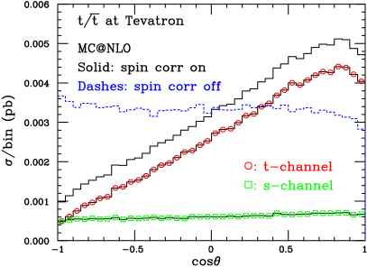
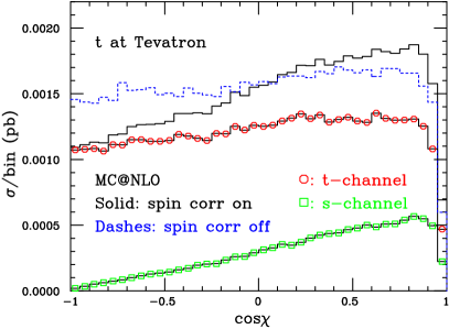
Figure 3: Angular correlations in single-top processes at the Tevatron: $\cos\theta$ in single-$t/\bar{t}$ production (left pane), and $\cos\chi$ in single-$t$ production (right pane). Histograms without symbols are the sums of $s$- and $t$-channel contributions.

Accordingly, we present in the left pane of fig. 3 the distribution in the cosine of the angle $\theta$, defined as the angle between the direction of flight of the lepton emerging from top decay, and the axis of the hardest jet which does not contain a stable $b$-flavoured hadron; the angle is defined in the rest frame of the top quark. This distribution has been shown in ref. [13] at tree level, and in ref. [14] at NLO using MCFM [6]. We have applied similar cuts as those in ref. [13], namely we required the decay products of the top to have

$$p_{\scriptscriptstyle\rm T}(b)\geq 20~{}{\rm GeV}\,,\;\;\;\;\;\;\left|\eta(b)\right|\leq 2\,,$$ (54)

$$p_{\scriptscriptstyle\rm T}(l)\geq 10~{}{\rm GeV}\,,\;\;\;\;\;\;\left|\eta(l)\right|\leq 2.5\,,$$ (55)

$$p_{\scriptscriptstyle\rm T}(\nu)\geq 20~{}{\rm GeV}\,.$$ (56)

We also require the hardest light jet to have transverse momentum larger than 20 GeV, and $\left|\eta(j)\right|\leq 2.5$. In this way, we obtain $A=-0.35$, where

$$A=\frac{\sigma(-1\leq\cos\theta<-0.1)-\sigma(-0.1\leq\cos\theta<0.8)}{\sigma(-1\leq\cos\theta<-0.1)+\sigma(-0.1\leq\cos\theta<0.8)}\,.$$ (57)

As can be seen from fig. 3, this result is due to the contribution of the $t$-channel, the $s$-channel having a very small asymmetry. We remark that the asymmetry is also compatible with zero if spin correlations are switched off. It is important to notice that our results follow the same pattern (and are actually close numerically) of those of refs. [13, 14]. Although we did not carry out a comprehensive study, this fact implies that not only is the $\cos\theta$ asymmetry fairly robust when including higher order corrections, but it is also stable when passing from a parton-level description such as that of refs. [13, 14] to a more realistic hadron-level description such as that of MC@NLO.

We conclude by presenting in the right pane of fig. 3 the distribution in the cosine of the angle $\chi$, which is defined analogously to the angle $\theta$, except for the fact that the reference direction is chosen to be that of the antiproton beam (at variance with the case of $\cos\theta$, we have limited ourselves here to considering $t$ production, rather than $t+\bar{t}$ production). As expected [12], the dominant contribution to the asymmetry is due in this case to the $s$-channel. An extremely small non-zero asymmetry may also be visible in the case in which angular correlations are not included; we have verified that this is an artifact of the cuts adopted in the present analysis.

5 Conclusions

We have presented a method for the efficient inclusion of angular correlations due to production spin correlations in Monte Carlo event generators. The method has been demonstrated in detail for vector boson and top quark decays, but it is in fact quite general, relying only on the fact that the matrix elements do not contain sharp features that would lead to unacceptably low efficiency. The method is exact, and equivalent to what is currently implemented in LO-accurate event generators such as HERWIG. When the event generator is matched to NLO predictions, as is the case for MC@NLO and POWHEG, the resulting correlations are correct to LO in soft and collinear regions and to NLO elsewhere. The method has been implemented in MC@NLO for $WW$, $t\bar{t}$ and single-top hadroproduction and leptonic decay, and we have presented illustrative results for the latter two cases. These results show that significant correlations are present in suitably chosen observables. Version 3.3 of MC@NLO implements off-shell effects only in the case of $WW$ production. Future versions will include off-shell effects in top decay; also, vector bosons and top quarks decaying hadronically can be simulated using the formalism presented here, bearing in mind that NLO corrections to decays are neglected.

Appendix A Upper bounds in vector boson production

In this appendix, we present an alternative derivation of eq. (31). One introduces the quantity

$$N^{\nu}\equiv M^{\mu}\frac{i}{q^{2}-m_{V}^{2}+im_{V}\Gamma_{V}}\left(-g_{\mu}^{\;\;\nu}+\frac{q_{\mu}q^{\nu}}{m_{V}^{2}}\right)\;,$$ (58)

with which eq. (18) becomes

$$\sum_{\rm spins}\left|A\right|^{2}=F_{V}^{2}\,{\rm Tr}\!\left[\left(V_{Vl}^{2}+A_{Vl}^{2}-2V_{Vl}A_{Vl}\gamma_{5}\right)/\!\!\!k_{1}\,/\!\!\!\!N\,/\!\!\!k_{2}\,/\!\!\!\!N^{*}\right].$$ (59)

Evaluating this in the rest-frame of the (virtual) vector boson, with the $z$-axis along the direction of the lepton 3-momentum, we find

$$\sum_{\rm spins}\left|A\right|^{2}=2q^{2}F_{V}^{2}\,\left[\left(V_{Vl}^{2}+A_{Vl}^{2}\right)\left(N^{1}N^{1*}+N^{2}N^{2*}\right)+4V_{Vl}A_{Vl}\,{\rm Im}\left(N^{1}N^{2*}\right)\right]\;.$$ (60)

To establish an upper bound on this quantity, we note that

$$2\left|{\rm Im}\left(N^{1}N^{2*}\right)\right|\leq 2\left|N^{1}\right|\,\left|N^{2}\right|\leq N^{1}N^{1*}+N^{2}N^{2*}$$ (61)

and so

$$\sum_{\rm spins}\left|A\right|^{2} \leq 2q^{2}F_{V}^{2}\,\left(\left|V_{Vl}\right|+\left|A_{Vl}\right|\right)^{2}\left(N^{1}N^{1*}+N^{2}N^{2*}\right)$$ (62)

$$= \frac{2q^{2}F_{V}^{2}\,\left(\left|V_{Vl}\right|+\left|A_{Vl}\right|\right)^{2}}{(q^{2}-m_{V}^{2})^{2}+(m_{V}\Gamma_{V})^{2}}\left(M^{1}M^{1*}+M^{2}M^{2*}\right)\;.$$

Note that $M^{1,2}$ in this expression are strictly off-mass-shell quantities: no on-shell approximations have been made at this stage.

Now consider the production of a stable vector boson of mass $m_{V}$. Denoting the amplitude for this by $\bar{A}$, we have (again in the vector boson rest frame)

$$\sum_{\rm spins}\left|\bar{A}\right|^{2} = \bar{M}^{\mu}\bar{M}^{\nu}\left(-g_{\mu\nu}+\frac{q_{\mu}q_{\nu}}{m_{V}^{2}}\right)_{q^{2}=m_{V}^{2}}$$ (63)

$$= \bar{M}^{1}\bar{M}^{1*}+\bar{M}^{2}\bar{M}^{2*}+\bar{M}^{3}\bar{M}^{3*}$$

where $\bar{M}^{\mu}$ denotes the on-mass-shell value of $M^{\mu}$. Therefore, as long as

$$M^{1}M^{1*}+M^{2}M^{2*}\leq\bar{M}^{1}\bar{M}^{1*}+\bar{M}^{2}\bar{M}^{2*}+\bar{M}^{3}\bar{M}^{3*}$$ (64)

we have

$$\sum_{\rm spins}\left|A\right|^{2}\leq\frac{2q^{2}F_{V}^{2}\,\left(\left|V_{Vl}\right|+\left|A_{Vl}\right|\right)^{2}}{(q^{2}-m_{V}^{2})^{2}+(m_{V}\Gamma_{V})^{2}}\sum_{\rm spins}\left|\bar{A}\right|^{2}$$ (65)

and hence

$$\frac{d\sigma_{l\overline{l}}}{d\Phi_{2+1^{\!\star}}}\leq\frac{2q^{2}F_{V}^{2}\,\left(\left|V_{Vl}\right|+\left|A_{Vl}\right|\right)^{2}}{(q^{2}-m_{V}^{2})^{2}+(m_{V}\Gamma_{V})^{2}}\frac{d\sigma_{V}}{d\Phi_{1+1^{\!\star}}}\;,$$ (66)

which is identical to eq. (31), given the fact that $V_{Vl}A_{Vl}>0$, and that both equations are valid on-shell.

Clearly, one may check whether the bounds given in eqs. (31) and (66) are not violated in the case of off-shell vector bosons. This is indeed the case, provided that the off-shellness is not too large or too small (typically, this happens within $\pm 30\Gamma_{V}$ of the pole mass). A good strategy is that of using eq. (31) for $q^{2}<m_{V}^{2}$, and eq. (66) for $q^{2}>m_{V}^{2}$. However, one should bear in mind that in the case of off-shell particles the values of Bjorken $x$’s, and hence of the PDFs, may change, thus potentially affecting the bound.

References

- [1] S. Frixione and B. R. Webber, “Matching NLO QCD computations and parton shower simulations,” JHEP 0206 (2002) 029 [hep-ph/0204244].
- [2] S. Frixione, P. Nason and B. R. Webber, “Matching NLO QCD and parton showers in heavy flavour production,” JHEP 0308 (2003) 007 [arXiv:hep-ph/0305252].
- [3] P. Nason, “A new method for combining NLO QCD with shower Monte Carlo algorithms,” JHEP 0411 (2004) 040 [arXiv:hep-ph/0409146].
- [4] E. Merzbacher, Quantum Mechanics, J. Wiley & Sons, 3rd edition (1997).
- [5] S. Frixione and B. R. Webber, “The MC@NLO 3.3 Event Generator,” arXiv:hep-ph/0612272.
- [6] J. Campbell, R. K. Ellis and F. Tramontano, “Single top production and decay at next-to-leading order,” Phys. Rev. D 70 (2004) 094012 [arXiv:hep-ph/0408158].
- [7] Q. H. Cao and C. P. Yuan, “Single top quark production and decay at next-to-leading order in hadron collision,” Phys. Rev. D 71 (2005) 054022 [arXiv:hep-ph/0408180].
- [8] P. Nason and G. Ridolfi, “A positive-weight next-to-leading-order Monte Carlo for Z pair hadroproduction,” JHEP 0608 (2006) 077 [arXiv:hep-ph/0606275].
- [9] A. D. Martin, R. G. Roberts, W. J. Stirling and R. S. Thorne, “Uncertainties of predictions from parton distributions. I: Experimental errors. ((T)),” Eur. Phys. J. C 28 (2003) 455 [arXiv:hep-ph/0211080].
- [10] S. Catani, Y. L. Dokshitzer, M. H. Seymour and B. R. Webber, “Longitudinally Invariant K(T) Clustering Algorithms For Hadron Hadron Collisions,” Nucl. Phys. B 406 (1993) 187.
- [11] W. Bernreuther, A. Brandenburg, Z. G. Si and P. Uwer, “Top quark pair production and decay at hadron colliders,” Nucl. Phys. B 690 (2004) 81 [arXiv:hep-ph/0403035].
- [12] G. Mahlon and S. J. Parke, “Improved spin basis for angular correlation studies in single top quark production at the Tevatron,” Phys. Rev. D 55, 7249 (1997) [arXiv:hep-ph/9611367].
- [13] T. Stelzer, Z. Sullivan and S. Willenbrock, “Single top quark production at hadron colliders,” Phys. Rev. D 58 (1998) 094021 [arXiv:hep-ph/9807340].
- [14] Z. Sullivan, “Angular correlations in single-top-quark and W j j production at next-to-leading order,” Phys. Rev. D 72 (2005) 094034 [arXiv:hep-ph/0510224].