Theoretical update of $B_{s}\!-\!\,\overline{\!B}{}_{s}\,$ mixing

Alexander Lenz

Institut für Theoretische Physik – Universität Regensburg

D-93040 Regensburg, Germany

and

Ulrich Nierste

Institut für Theoretische Teilchenphysik – Universität Karlsruhe

D-76128 Karlsruhe, Germany

Abstract

We update the theory predictions for the mass difference $\Delta M_{s}$, the width difference $\Delta\Gamma_{s}$ and the CP asymmetry in flavour-specific decays, $a_{\rm fs}^{s}$, for the $B_{s}\!-\!\,\overline{\!B}{}_{s}\,$ system. In particular we present a new expression for the element $\Gamma_{12}^{s}$ of the decay matrix, which enters the predictions of $\Delta\Gamma_{s}$ and $a_{\rm fs}^{s}$. To this end we introduce a new operator basis, which reduces the troublesome sizes of the $1/m_{b}$ and $\alpha_{s}$ corrections and diminishes the hadronic uncertainty in $\Delta\Gamma_{s}/\Delta M_{s}$ considerably. Logarithms of the charm quark mass are summed to all orders. We find $\Delta\Gamma_{s}/\Delta M_{s}=(49.7\pm 9.4)\cdot 10^{-4}$ and $\Delta\Gamma_{s}=(f_{B_{s}}/240\,{\rm MeV})^{2}[(0.105\pm 0.016)\,B\;+\;(0.024\pm 0.004)\,\tilde{B}_{S}^{\prime}\;-\;0.027\pm 0.015]\,\mbox{ps}^{-1}$ in terms of the bag parameters $B$, $\tilde{B}_{S}^{\prime}$ in the NDR scheme and the decay constant $f_{B_{s}}$. The improved result for $\Gamma_{12}^{s}$ also permits the extraction of the CP-violating $B_{s}\!-\!\,\overline{\!B}{}_{s}\,$ mixing phase from $a_{\rm fs}^{s}$ with better accuracy. We show how the measurements of $\Delta M_{s}$, $\Delta\Gamma_{s}$, $a_{\rm fs}^{s}$, $A_{\rm CP}^{\rm mix}(B_{s}\to J/\psi\phi)$ and other observables can be efficiently combined to constrain new physics. Applying our new formulae to data from the DØ experiment, we find a 2$\sigma$ deviation of the $B_{s}\!-\!\,\overline{\!B}{}_{s}\,$ mixing phase from its Standard Model value. We also briefly update the theory predictions for the $B_{d}\!-\!\,\overline{\!B}{}_{d}\,$ system and find $\Delta\Gamma_{d}/\Delta M_{d}=\left(52.6\raisebox{-2.15277pt}{\shortstack[l]{$\scriptstyle+11.5$\\ $\scriptstyle-12.8$}}\right)\,\cdot 10^{-4}$ and $a_{\rm fs}^{d}=\left(-4.8\raisebox{-2.15277pt}{\shortstack[l]{$\scriptstyle+1.0$\\ $\scriptstyle-1.2$}}\right)\,\cdot 10^{-4}$ in the Standard Model.

PACS numbers: 12.38.Bx, 13.25.Hw, 11.30Er, 12.60.-i

1 Introduction

Flavour-changing neutral current (FCNC) processes are highly sensitive to new physics around the TeV scale. Global fits to the unitarity triangle show an excellent agreement of $b\to d$ and $s\to d$ transitions with the predictions of the Cabibbo-Kobayashi-Maskawa (CKM) mechanism [1, 2]. Extensions of the Standard Model can contain sources of flavour-changing transitions beyond the CKM matrix. Models without these new sources are termed to respect minimal flavour violation (MFV). Despite of the success of the MFV hypothesis in $b\to d$ and $s\to d$ transitions there is still sizable room for non-MFV contribution in $b\to s$ transitions. For instance, an extra contribution to $b\to s\overline{q}q$, $q=u,d,s$, decay amplitudes with a CP phase different from $\arg(V_{ts}^{*}V_{tb})$ can alleviate the $\sim 2.6\sigma$ discrepancy between the measured mixing-induced CP asymmetries in these $b\to s$ penguin modes and the Standard Model prediction [3]. Models of supersymmetric grand unification can naturally accommodate new contributions to $b\to s$ transitions [4]: right-handed quarks reside in the same quintuplets of SU(5) as left-handed neutrinos, so that the large atmospheric neutrino mixing angle could well affect squark-gluino mediated $b\to s$ transitions [5].

Clearly, $B_{s}\!-\!\,\overline{\!B}{}_{s}\,$ mixing plays a preeminent role in the search for new physics in $b\to s$ FCNC’s. $B_{s}\!-\!\,\overline{\!B}{}_{s}\,$ oscillations are governed by a Schrödinger equation

$$i\frac{d}{dt}\left(\begin{array}[]{c}|B_{s}(t)\rangle\\ |\bar{B}_{s}(t)\rangle\end{array}\right)=\left(M^{s}-\frac{i}{2}\Gamma^{s}\right)\left(\begin{array}[]{c}|B_{s}(t)\rangle\\ |\bar{B}_{s}(t)\rangle\end{array}\right)$$ (1)

with the mass matrix $M^{s}$ and the decay matrix $\Gamma^{s}$. The physical eigenstates $|B_{H}\rangle$ and $|B_{L}\rangle$ with the masses $M_{H},\,M_{L}$ and the decay rates $\Gamma_{H},\,\Gamma_{L}$ are obtained by diagonalizing $M^{s}-i\Gamma^{s}/2$. The $B_{s}\!-\!\,\overline{\!B}{}_{s}\,$ oscillations in Eq. (1) involve the three physical quantities $|M_{12}^{s}|$, $|\Gamma_{12}^{s}|$ and the CP phase $\phi_{s}=\arg(-M_{12}^{s}/\Gamma_{12}^{s})$ (see e.g. [6]). The mass and width differences between $B_{L}$ and $B_{H}$ are related to them as

$$\Delta M_{s} = M^{s}_{H}-M^{s}_{L}\;=\;2\,|M_{12}^{s}|,\qquad\Delta\Gamma_{s}\;=\;\Gamma^{s}_{L}-\Gamma^{s}_{H}\;=\;2\,|\Gamma_{12}^{s}|\cos\phi_{s},$$ (2)

up to numerically irrelevant corrections of order $m_{b}^{2}/M_{W}^{2}$. $\Delta M_{s}$ simply equals the frequency of the $B_{s}\!-\!\,\overline{\!B}{}_{s}\,$ oscillations. A third quantity providing independent information on the mixing problem in Eq. (1) is

$$a^{s}_{\rm fs} = \mathrm{Im}\,\frac{\Gamma_{12}^{s}}{M_{12}^{s}}\;=\;\frac{|\Gamma_{12}^{s}|}{|M_{12}^{s}|}\sin\phi_{s}\;=\;\frac{\Delta\Gamma_{s}}{\Delta M_{s}}\tan\phi_{s}.$$ (3)

$a_{\rm fs}^{s}$ is the CP asymmetry in flavour-specific $B_{s}\to f$ decays, which means that the decays $\,\overline{\!B}_{s}\to f$ and $B_{s}\to\overline{f}$ (with $\overline{f}$ denoting the CP-conjugate final state) are forbidden [7]. The standard way to access $a_{\rm fs}^{s}$ uses $B_{s}\to X_{s}\ell^{+}\overline{\nu_{\ell}}$ decays, which justifies the name semileptonic CP asymmetry for $a_{\rm fs}^{s}$. (See e.g. [6, 8] for more details on the phenomenology of $B_{s}\!-\!\,\overline{\!B}{}_{s}\,$ mixing.)

It is important to note that new physics can significantly affect $M_{12}^{s}$, but not $\Gamma_{12}^{s}$, which is dominated by the CKM-favoured $b\to c\overline{c}s$ tree-level decays. Hence all possible effects of new physics can be parameterised by two real parameters only, for instance $|M_{12}^{s}|$ and $\phi_{s}$. While $|M_{12}^{s}|$ is directly related to $\Delta M_{s}$, the extraction of $\phi_{s}$ from either $\Delta\Gamma_{s}$ or $a_{\rm fs}^{s}$ requires an accurate knowledge of $\Gamma_{12}^{s}$.

In the Standard Model $M_{12}^{s}$ and $\Gamma_{12}^{s}$ are computed from the box diagrams in Fig. 1 and QCD corrections in the desired order.

 

Figure 1: In the lowest order $M_{12}^{s}$ is calculated from the dispersive parts of the box diagrams on the left. It is dominated by the top contribution. The result involves only one local $|\Delta B|=2$ operator, shown in the right picture. The leading contribution to $\Gamma_{12}^{s}$ is obtained from the absorptive parts of the box diagrams on the left, to which only diagrams without top quark line contribute. To lowest order in the heavy quark expansion two $|\Delta B|=2$ operators occur, the $\overline{\Lambda}/m_{b}$ corrections involve five more.

 

The Standard Model prediction for $M_{12}$ reads:

$$M_{12} = \frac{G_{F}^{2}M_{B_{s}}}{12\pi^{2}}\,M_{W}^{2}\,(V_{tb}V_{ts}^{*})^{2}\,\widehat{\eta}_{B}\,S_{0}(x_{t})\,f_{B_{s}}^{2}B,$$ (4)

where $G_{F}$ is the Fermi constant, the $V_{ij}$’s are CKM elements, $M_{B_{s}}$ and $M_{W}$ are the masses of $B_{s}$ meson and W boson and the short-distance information is contained in $\widehat{\eta}_{B}\,S_{0}(x_{t})$: $S_{0}(x_{t})$ is the Inami-Lim function, which depends on the top mass $m_{t}$ through $x_{t}=m_{t}^{2}/M_{W}^{2}$, and $\widehat{\eta}_{B}$ is a numerical factor containing the leading and next-to-leading QCD corrections [9]. The calculation of $M_{12}$ involves the four-quark operator ($\alpha,\beta=1,2,3$ are colour indices):

$$Q = \overline{s}_{\alpha}\gamma_{\mu}(1-\gamma_{5})b_{\alpha}\,\overline{s}_{\beta}\gamma^{\mu}(1-\gamma_{5})b_{\beta}.$$ (5)

All long-distance QCD effects are contained in the hadronic matrix element of $Q$ and are parameterised by $f_{B_{s}}^{2}B$:

$$\langle B_{s}|Q|\overline{B}_{s}\rangle = \frac{8}{3}M^{2}_{B_{s}}\,f^{2}_{B_{s}}B.$$ (6)

The recent observation of the $B_{s}\!-\!\,\overline{\!B}{}_{s}\,$ mixing frequency $\Delta M_{s}=2|M_{12}^{s}|$ at the Tevatron [10] yields a powerful constraint on extensions of the Standard Model [11, 12, 13, 14]. The results from the DØ and CDF experiments obtained with 1 fb^-1 of data, are [15]

$$17\,\mbox{ps}^{-1}\leq\Delta M_{s} \leq 21\,\mbox{ps}^{-1}\qquad\qquad\quad@90\%\,\mbox{CL}\quad\qquad\mbox{D\O}$$

$$\Delta M_{s} = 17.77\pm{0.10}{}_{\mbox{\scriptsize(syst)}}\pm 0.07\,{}_{\mbox{\scriptsize(stat)}}\,\mbox{ps}^{-1}\,\qquad\mbox{CDF}.$$ (7)

While the precise measurement in Eq. (7) sharply determines $|M_{12}^{s}|$, the uncertainty of $f_{B_{s}}^{2}B$, which is around $30\%$, blurs the extraction of some new physics contribution adding to $S_{0}(x_{t})$ in Eq. (4). Alternatively one can study the ratio $\Delta M_{d}/\Delta M_{s}$, where $\Delta M_{d}$ is the mass difference in the $B_{d}\!-\!\,\overline{\!B}{}_{d}\,$ system. While the hadronic uncertainty in the ratio $f_{B_{s}}^{2}B/(f_{B_{d}}^{2}B_{B_{d}})$ is smaller, one is now dependent on $|V_{td}/V_{ts}|^{2}$. Even if one assumes non-standard contributions only in $B_{s}$ physics, but not in the quantities entering the global fit of the unitarity triangle, $|V_{td}/V_{ts}|^{2}$ is only known to roughly $40\%$ [2] leaving equally much room for new physics in $|M_{12}^{s}|$.

Adding experimental information from $\Delta\Gamma_{s}$ or $a_{\rm fs}^{s}$ helps in two ways; first, one can study the CP-violating phase $\phi_{s}$, which is totally unconstrained by $\Delta M_{s}$, through Eqs. (2) and (3). Second, one expects cancellations of hadronic parameters in the ratio $\Gamma_{12}^{s}/M_{12}^{s}$, which enters $a_{\rm fs}^{s}$ and $\Delta\Gamma_{s}/\Delta M_{s}$. All decays into final states with zero strangeness contribute to $\Gamma_{12}^{s}$, which is dominated by the CKM-favoured $b\to c\overline{c}s$ tree-level contribution. In the first step of the calculation the W-boson is integrated out and the W-mediated $|\Delta B|=1$ transitions are described by the usual effective $|\Delta B|=1$ hamiltonian with the current-current operators $Q_{1}$, $Q_{2}$ and the penguin operators $Q_{3-6}$, $Q_{8}$ [16]. The leading contribution to $\Gamma_{12}^{s}$ in this effective $|\Delta B|=1$ theory is shown in Fig. 2.

 

Figure 2: Leading-order CKM-favoured contribution to $\Gamma_{12}^{s}$, which arises from $\raisebox{7.7pt}{$\scriptscriptstyle(\hskip 8.5pt)$}\!\,\overline{\!B}_{s}$ decays to final states (indicated by the dashed lines) with a $(c,\overline{c})$ pair and zero strangeness. The crosses denote any of the operators $Q_{1-6}$ of the $|\Delta B|=1$ hamiltonian. The Cabibbo-suppressed contributions correspond to diagrams with one or both $c$ quarks replaced by $u$ quarks.

 

In the second step one uses an operator product expansion (OPE), the Heavy Quark Expansion (HQE), to express $\Gamma_{12}^{s}$ as an expansion in the two parameters $\overline{\Lambda}/m_{b}$ and $\alpha_{s}(m_{b})$. Here $\alpha_{s}$ is the QCD coupling constant and $\overline{\Lambda}$ is the appropriate hadronic scale, which quantifies the size of the hadronic matrix elements. The HQE links the diagrams of Fig. 2 to the matrix elements of local $\Delta B=2$ operators. In addition to the operator $Q$ in Eq. (5) one also encounters

$$Q_{S} = \overline{s}_{\alpha}(1+\gamma_{5})b_{\alpha}\,\overline{s}_{\beta}(1+\gamma_{5})b_{\beta},$$ (8)

whose matrix element is parameterised by a bag parameter $B_{S}$ in analogy to Eq. (6). The leading contribution to $\Gamma_{12}^{s}$ was obtained in [7, 17]. Today $\Gamma_{12}^{s}$ is known to next-to-leading-order (NLO) in both $\overline{\Lambda}/m_{b}$ [18] and $\alpha_{s}(m_{b})$ [19, 20]. The 1998 result [19]

$$\left(\frac{\Delta\Gamma_{s}}{\Gamma_{s}}\right)=\left(\frac{f_{B_{s}}}{210~{}{\rm MeV}}\right)^{2}\left[0.006\,B+0.150\,B_{S}-0.063\right]$$ (9)

with the average total width $\Gamma_{s}=(\Gamma^{s}_{L}+\Gamma^{s}_{H})/2$ is pathological in several respects: first, the $\overline{\Lambda}/m_{b}$ correction -0.063 is unnaturally large and amounts to around 40% of the total result. Second, the coefficient of $B$ cancels almost completely, the result is therefore dominated by the term proportional to $B_{S}\sim 0.9$, so that the cancellation of hadronic quantities from the ratio $\Delta\Gamma_{s}/\Delta M_{s}$ is very imperfect. Third, both the $\overline{\Lambda}/m_{b}$ and $\alpha_{s}$ corrections, which diminish the coefficient of $B_{S}$ from 0.22 to 0.15, are negative, and these numerical cancellations between leading-order (LO) order result and corrections increase the relative uncertainty of the prediction for $\Delta\Gamma_{s}/\Gamma_{s}$. In the following section we argue that these pathologies are caused by a poor choice of the operator basis used in [18, 19, 20] and propose a different basis. We also improve the prediction of $\Delta\Gamma_{s}/\Delta M_{s}$ and $\Delta\Gamma_{s}/\Gamma_{s}$ in several other aspects, by summing logarithms of the charm mass to all orders in $\alpha_{s}$, by using different renormalisation schemes for the $b$-quark mass, by including CKM-suppressed contributions and by modifying the normalisation related to the factor $1/\Gamma_{s}$ in Eq. (9). In Sect. 3 we present numerical updates first of $\Delta M_{s}$, $\Delta\Gamma_{s}$ and $a_{\rm fs}^{s}$ and then of the corresponding quantities in the $B_{d}$-system. In Sect. 4 we show how the expressions for the mixing quantities change in the presence of new physics. Here we discuss how to combine different present and future measurements to constrain $|M_{12}^{s}|$ and $\phi_{s}$ and advocate a novel method to display the constraints on possible new short-distance physics in $B_{s}\!-\!\,\overline{\!B}{}_{s}\,$ mixing. Sect. 5 gives a road map for future measurements and calculations and Sect. 6 summarises our results.

2 Improved prediction of $\Gamma_{12}^{s}$

We write $\Gamma_{12}^{s}$ as [21]

$$\Gamma_{12}^{s} = -\left[\,\lambda_{c}^{2}\,\Gamma_{12}^{cc}\;+\;2\,\lambda_{c}\,\lambda_{u}\,\Gamma_{12}^{uc}\;+\;\lambda_{u}^{2}\,\Gamma_{12}^{uu}\,\right]$$ (10)

$$= -\left[\,\lambda_{t}^{2}\,\Gamma_{12}^{cc}\;+\;2\,\lambda_{t}\,\lambda_{u}\,\left(\Gamma_{12}^{cc}-\Gamma_{12}^{uc}\right)\;+\;\lambda_{u}^{2}\,\left(\Gamma_{12}^{cc}-2\Gamma_{12}^{uc}+\Gamma_{12}^{uu}\right)\right]$$ (11)

with the CKM factors $\lambda_{i}=V_{is}^{*}V_{ib}$ for $i=u,c,t$. In Eq. (11) we have eliminated $\lambda_{c}$ in favour of $\lambda_{t}$ using $\lambda_{u}+\lambda_{c}+\lambda_{t}=0$ to prepare for the study of $\Gamma_{12}^{s}/M_{12}^{s}$. Since $|\lambda_{u}|\ll|\lambda_{t}|\approx|\lambda_{c}|$, $\Gamma_{12}^{cc}$ clearly dominates $\Gamma_{12}^{s}$. For $ab=cc,uc,uu$ we write [19, 21]

$$\Gamma_{12}^{ab} = \frac{G_{F}^{2}m_{b}^{2}}{24\pi\,M_{B_{s}}}\left[\,G^{ab}\,\langle B_{s}|Q|\,\overline{\!B}_{s}\rangle\;-\;G_{S}^{ab}\,\langle B_{s}|Q_{S}|\,\overline{\!B}_{s}\rangle\right]\;+\;\Gamma_{12,1/m_{b}}^{ab}$$ (12)

The coefficients $G^{ab}$ and $G_{S}^{ab}$ are further decomposed as

$$G^{ab}\;=\;F^{ab}+P^{ab},\qquad G_{S}^{ab}\;=\;-F_{S}^{ab}-P_{S}^{ab}.$$ (13)

Here $F^{ab}$ and $F_{S}^{ab}$ are the contributions from the current-current operators $Q_{1,2}$ while the small coefficients $P^{ab}$ and $P_{S}^{ab}$ stem from the penguin operators $Q_{3-6}$ and $Q_{8}$. (Note that in [19], where only the dominant $\Gamma_{12}^{cc}$ was considered, these coefficients had no superscript ’cc’.) Numerical cancellations render $F^{cc}$ small with $|F^{cc}/F_{S}^{cc}|\approx 0.03$ which explains the small coefficient of $B$ in Eq. (9).

We parameterise the matrix element of $Q_{S}$ as

$$\langle B_{s}|Q_{S}|\,\overline{\!B}_{s}\rangle = -\frac{5}{3}M^{2}_{B_{s}}\,f^{2}_{B_{s}}B_{S}^{\prime}.$$ (14)

Formulae for physical quantities are more compact when expressed in terms of $B_{S}^{\prime}$ rather than the conventionally used bag parameter $B_{S}$. The two parameters are related as

$$B_{S}^{\prime} = \frac{M^{2}_{B_{s}}}{(\overline{m}_{b}+\overline{m}_{s})^{2}}B_{S}.$$ (15)

In the vacuum insertion approximation (VIA) the bag factors $B$ and $B_{S}$ are equal to one. Throughout this paper we use the $\overline{\rm MS}$ scheme as defined in [19, 21] for all operators. Therefore the masses $\overline{m}_{b}$ and $\overline{m}_{s}$ appearing in Eq. (15) correspond to the $\overline{\rm MS}$ scheme as well.

$\Gamma_{12,1/m_{b}}^{cc}$ comprises effects suppressed by $\overline{\Lambda}/m_{b}$. We will discuss it later, after transforming to our new operator basis.

2.1 New operator basis

When calculating $\Gamma_{12}$ to leading order in $\overline{\Lambda}/m_{b}$, one first encounters a third operator $\widetilde{Q}_{S}$ in addition to $Q$ and $Q_{S}$ defined in Eqs. (5) and (8):

$$\widetilde{Q}_{S} = \overline{s}_{\alpha}(1+\gamma_{5})b_{\beta}\,\overline{s}_{\beta}(1+\gamma_{5})b_{\alpha},$$ (16)

However, a certain linear combination of $Q$, $Q_{S}$ and $\widetilde{Q}_{S}$ is a $1/m_{b}$–suppressed operator [18]. This $1/m_{b}$–suppressed operator reads

$$R_{0} \equiv Q_{S}\;+\;\alpha_{1}\tilde{Q}_{S}\;+\;\frac{1}{2}\alpha_{2}Q,$$ (17)

where $\alpha_{1,2}$ contain NLO corrections, which are specific to the $\overline{\rm MS}$ scheme used by us [19]:

$$\!\!\alpha_{1}\;=\;1\;+\;\frac{\alpha_{s}(\mu_{2})}{4\pi}\,C_{f}\left(12\ln\frac{\mu_{2}}{m_{b}}+6\right), \;\alpha_{2}\;=\;1\;+\;\frac{\alpha_{s}(\mu_{2})}{4\pi}\,C_{f}\left(6\ln\frac{\mu_{2}}{m_{b}}+\frac{13}{2}\right).$$ (18)

Here $C_{f}=4/3$ is a colour factor and $\mu_{2}$ is the scale at which the operators in Eq. (17) are defined. The coefficients $G$ and $G_{S}$ in Eq. (12) depend on $\mu_{2}$ and this dependence cancels with the $\mu_{2}$–dependence of $\langle B_{s}|Q(\mu_{2})|\overline{B}_{s}\rangle$ and $\langle B_{s}|Q_{S}(\mu_{2})|\overline{B}_{s}\rangle$. In lattice computations the $\mu_{2}$–dependence enters in the lattice–continuum matching of these matrix elements. In our numerics we will always quote the results for $\mu_{2}=m_{b}$. In [18, 19, 20] Eq. (17) has been used to eliminate $Q_{S}$ in favour of $R_{0}$ leading to the result in Eq. (9). The matrix element of $\widetilde{Q}_{S}$ reads

$$\langle B_{s}|\widetilde{Q}_{S}(\mu_{2})|\overline{B}_{s}\rangle = \frac{1}{3}M^{2}_{B_{s}}\,f^{2}_{B_{s}}\widetilde{B}_{S}^{\prime}(\mu_{2}).$$ (19)

In analogy to Eq. (15) we define

$$\widetilde{B}_{S}^{\prime}(\mu_{2}) = \frac{M^{2}_{B_{s}}}{(\overline{m}_{b}(\mu_{2})+\overline{m}_{s}(\mu_{2}))^{2}}\widetilde{B}_{S}(\mu_{2}).$$ (20)

For clarity we have explicitly shown the $\mu_{2}$-dependence in Eqs. (19) and (20), which was skipped in Eqs. (6),(14) and (15). In VIA $\widetilde{B}_{S}=1$ and $\langle B_{s}|\widetilde{Q}_{S}|\overline{B}_{s}\rangle$ is much smaller than $\langle B_{s}|Q|\overline{B}_{s}\rangle$ and $\langle B_{s}|Q_{S}|\overline{B}_{s}\rangle$. The small coefficient $1/3$ in Eq. (19) is the consequence of a cancellation between the leading term in the $1/N_{c}$ expansion, where $N_{c}=3$ is the number of colours, and the factorisable $1/N_{c}$ corrections: $1/3=1-2/N_{c}$. One naturally expects that the bag factor $\widetilde{B}_{S}$ substantially deviates from 1. However, a lattice computation found $\widetilde{B}_{S}=0.91\pm 0.08$ [22], showing that the matrix element of $\widetilde{Q}_{S}$ is indeed small. Thus $\langle B_{s}|R_{0}|\overline{B}_{s}\rangle=\overline{\Lambda}/m_{b}$ implies a strong numerical relationship between $B$ and $B_{S}$ which can be used to constrain $B_{S}/B$ entering $\Delta\Gamma_{s}/\Delta M_{s}$. Yet it is more straightforward to use Eq. (17) to eliminate $Q_{S}$ altogether from $\Gamma_{12}$ in favour of $\widetilde{Q}_{S}$. The coefficient of $B$ will change and and the coefficient of $\widetilde{B}_{S}^{\prime}$ is expected to be small in view of the factor of 1/3 in Eq. (19). Using further the bag parameters of Eqs. (6) and (14), $\Gamma_{12}^{ab}$ of Eq. (12) now reads

$$\Gamma_{12}^{ab} = \frac{G_{F}^{2}m_{b}^{2}}{24\pi}\,M_{B_{s}}\,f^{2}_{B_{s}}\,\left[\,\left(G^{ab}+\frac{\alpha_{2}}{2}G_{S}^{ab}\right)\,\frac{8}{3}B\;+\;G_{S}^{ab}\alpha_{1}\,\frac{1}{3}\widetilde{B}_{S}^{\prime}\right]\;+\;\widetilde{\Gamma}_{12,1/m_{b}}^{ab}.$$ (21)

The new $1/m_{b}$–corrections are related to $\Gamma_{12,1/m_{b}}^{ab}$ appearing in Eq. (12) as

$$\widetilde{\Gamma}_{12,1/m_{b}}^{ab} = \Gamma_{12,1/m_{b}}^{ab}\;+\;\frac{G_{F}^{2}m_{b}^{2}}{24\pi\,M_{B_{s}}}\,F_{S}^{ab,(0)}\,\langle B_{s}|R_{0}|\overline{B}_{s}\rangle.$$ (22)

Here we have taken into account that the result of [19, 20] includes the $\overline{\Lambda}/m_{b}$ terms without penguin contributions and to LO in $\alpha_{s}$: consequently we have changed $-G_{S}^{ab}$ to $F_{S}^{ab,(0)}$, which is the LO approximation to $F_{S}^{ab}$. Recalling $|G^{ab}|\ll|G_{S}^{ab}|$ and $B,\widetilde{B}_{S}^{\prime}\approx 1$ one easily verifies from Eq. (21) that the first term proportional to $B$ dominates over the second term. Since $\Gamma_{12,1/m_{b}}^{ab}$ in Eq. (9) is negative and the shift in Eq. (22) adds a positive term our change of basis also leads to $|\widetilde{\Gamma}_{12,1/m_{b}}^{ab}|<|\Gamma_{12,1/m_{b}}^{ab}|$. Further the $\alpha_{s}$-corrections contained in $\alpha_{1,2}$, which multiply $G_{S}^{ab,(0)}$ in Eq. (21), temper the large NLO corrections of the old result. These three effects combine to reduce the hadronic uncertainty in $\Delta\Gamma_{s}/\Delta M_{s}$ substantially. In other words: the uncertainty quoted in [19, 20] is not intrinsic to $\Delta\Gamma_{s}/\Delta M_{s}$ but an artifact of a poorly chosen operator basis.

2.2 A closer look at $\mathbf{1/m_{b}}$ corrections

At order $1/m_{b}$ one encounters the operators $R_{0}$ of Eq. (17),

$$R_{1} = \frac{m_{s}}{m_{b}}\;\overline{s}_{\alpha}(1+\gamma_{5})b_{\alpha}\,\overline{s}_{\beta}(1-\gamma_{5})b_{\beta}$$

$$R_{2} = \frac{1}{m^{2}_{b}}\;\overline{s}_{\alpha}{\overleftarrow{D}}_{\!\rho}\gamma^{\mu}(1-\gamma_{5})D^{\rho}b_{\alpha}\,\overline{s}_{\beta}\gamma_{\mu}(1-\gamma_{5})b_{\beta}$$

$$R_{3} = \frac{1}{m^{2}_{b}}\;\overline{s}_{\alpha}{\overleftarrow{D}}_{\!\rho}(1+\gamma_{5})D^{\rho}b_{\alpha}\,\overline{s}_{\beta}(1+\gamma_{5})b_{\beta}$$ (23)

and the operators $\widetilde{R}_{i}$ which are obtained from the $R_{i}$’s by interchanging the colour indices $\alpha$ and $\beta$ of the two $s$ fields [18]. At order $1/m_{b}$ only five of these operators are independent because of relations like $\widetilde{R}_{2}=-R_{2}+{\cal O}(1/m_{b}^{2})$. Writing (for $ab=cc,uc,uu$)

$$\widetilde{\Gamma}_{12,1/m_{b}}^{ab} = \frac{G_{F}^{2}m_{b}^{2}}{24\pi M_{B_{s}}}\left[g_{0}^{ab}\langle B_{s}|R_{0}|\overline{B}_{s}\rangle\,+\,\sum_{j=1}^{3}\left[g_{j}^{ab}\langle B_{s}|R_{j}|\overline{B}_{s}\rangle+\widetilde{g}_{j}^{ab}\langle B_{s}|\widetilde{R}_{j}|\overline{B}_{s}\rangle\right]\right]$$ (24)

the coefficients $g_{j}^{ab}$ and $\widetilde{g}_{j}^{ab}$ read [18, 23, 21]:

$$g_{0}^{cc}\;=\;\sqrt{1-4z}(1+2z)C_{2}^{(0)\,2}\,+\,F_{S}^{cc\,(0)}\;= \!\!\!\!\!\sqrt{1-4z}\,(1+2z)\,C_{1}^{(0)}\left[3C_{1}^{(0)}\,+\,2\,C_{2}^{(0)}\right]$$

$$g_{1}^{cc}\;=\;-2\sqrt{1-4z}(1+2z)\,C_{1}^{(0)}\,\left[3C_{1}^{(0)}\,+\,2C_{2}^{(0)}\right] \quad\widetilde{g}_{1}^{cc}\;=\;-2\sqrt{1-4z}(1+2z)C_{2}^{(0)\,2}$$

$$g_{2}^{cc}\;=\;-2\,\frac{1-2z-2z^{2}}{\sqrt{1-4z}}\,C_{1}^{(0)}\,\left[3C_{1}^{(0)}\,+\,2C_{2}^{(0)}\right] \quad\widetilde{g}_{2}^{cc}\;=\;-2\,\frac{1-2z-2z^{2}}{\sqrt{1-4z}}C_{2}^{(0)\,2}$$

$$g_{3}^{cc}\;=\;-24\,\frac{z^{2}}{\sqrt{1-4z}}\,C_{1}^{(0)}\left[3C_{1}^{(0)}\,+\,2C_{2}^{(0)}\right] \quad\widetilde{g}_{3}^{cc}\;=\;-24\,\frac{z^{2}}{\sqrt{1-4z}}C_{2}^{(0)\,2}$$ (25)

$$g_{0}^{uc}\;=\;(1-z)^{2}(1+2z)C_{2}^{(0)\,2}\,+\,F_{S}^{uc\,(0)}\,= \!\!\!\!\!\!\!(1-z)^{2}\,(1+2z)\,C_{1}^{(0)}\left[3C_{1}^{(0)}\,+\,2\,C_{2}^{(0)}\right]$$

$$g_{1}^{uc}\;=\;-2(1-z)^{2}(1+2z)\,C_{1}^{(0)}\,\left[3C_{1}^{(0)}\,+\,2C_{2}^{(0)}\right] \widetilde{g}_{1}^{uc}\;=\;-2(1-z)^{2}(1+2z)C_{2}^{(0)\,2}$$

$$g_{2}^{uc}\;=\;-2\,(1-z)\,(1+z+z^{2})\,C_{1}^{(0)}\,\left[3C_{1}^{(0)}\,+\,2C_{2}^{(0)}\right] \widetilde{g}_{2}^{uc}\;=\;-2\,(1-z)\,(1+z+z^{2})C_{2}^{(0)\,2}$$

$$g_{3}^{uc}\;=\;-12\,(1-z)\,z^{2}\,C_{1}^{(0)}\left[3C_{1}^{(0)}\,+\,2C_{2}^{(0)}\right] \widetilde{g}_{3}^{uc}\;=\;-12\,(1-z)\,z^{2}\,C_{2}^{(0)\,2}.$$ (26)

and $g_{j}^{uu}=g_{j}^{cc}(z=0)=g_{j}^{uc}(z=0)$. Here

$$z \equiv \frac{\overline{m}_{c}^{2}}{\overline{m}_{b}^{2}}\;\equiv\;\frac{\left[\overline{m}_{c}(\overline{m}_{c})\right]^{2}}{\left[\overline{m}_{b}(\overline{m}_{b})\right]^{2}}$$ (27)

and $C_{1}^{(0)}\sim-0.3$ and $C_{2}^{(0)}\sim 1.1$ are the LO Wilson coefficients of the $\Delta B=1$ operators $Q_{1}$ and $Q_{2}$ [16].

The contributions involving $R_{1}$, $\widetilde{R}_{1}$, $R_{3}$ and $\widetilde{R}_{3}$ are suppressed by powers of $m_{s}/m_{b}$ or $z^{2}$ and are numerically negligible. The only two important $1/m_{b}$ operators are $R_{0}$ and $\widetilde{R}_{2}=-R_{2}+{\cal O}(1/m_{b}^{2})$. As a consequence of the elimination of $Q_{S}$ in favour of $\widetilde{Q}_{S}$ no term involving the large coefficient $C_{2}^{(0)\,2}$ occurs in $g_{0}^{ab}$. The contribution from $R_{0}$ is substantially diminished, and this can be understood in terms of a systematic expansion in $1/N_{c}$: the coefficients $g_{0}^{ab}$ are colour–suppressed due to $C_{1}\sim 1/N_{c}$, while they were colour–favoured in the old basis. Since radiative corrections cannot change the colour counting, this feature must persist in the yet uncalculated order $\alpha_{s}/m_{b}$. In other words, by changing to our new basis we have absorbed the corrections of order $N_{c}^{0}/m_{b}$ into the leading order of the $1/m_{b}$ expansion. This improves our result over the one in the old basis by a term of order $N_{c}\alpha_{s}/m_{b}$. (Recall that $\alpha_{s}\sim 1/N_{c}$, so that $N_{c}\alpha_{s}/m_{b}\sim N_{c}^{0}/m_{b}$.) This term (which constitutes a parametrically enhanced correction) would appear, if the calculation of $\alpha_{s}/m_{b}$ were done in the old basis. In fact, this term occurs in the NLO calculation of [19, 20, 21] in the coefficient of $\widetilde{Q}_{S}$ but is dropped once $\widetilde{Q}_{S}$ is traded for $R_{0}$, because all $\alpha_{s}/m_{b}$ terms are consistently discarded. With the use of our new basis no corrections of order $N_{c}\alpha_{s}/m_{b}$ to $g_{0}^{ab}$ can occur. This feature can also be understood by realising that the large–$N_{c}$ contribution to $\Gamma_{12}^{ab}$ stems from the right diagram in Fig. 2 with two insertions of $Q_{2}$ plus additional planar graphs with extra gluons. These diagrams contribute to the coefficients of $Q$ and $\widetilde{Q}_{S}$, but not to the coefficient of $Q_{S}$. (This is easy to see, if one inserts the two $Q_{2}$’s in the Fierz-rearranged form.) Upon elimination of $Q_{S}$ in favour of $R_{0}$, the color–suppressed coefficient $g^{ab}$ of $Q_{S}$ becomes the coefficient of $R_{0}$. At order $1/m_{b}$ one has to include the momentum of the $s$ quark in that diagram and finds a contribution to the $\widetilde{g}_{i}^{ab}$’s at order $N_{c}^{0}$. These terms are identical in both bases. Our numerical analysis in Sect. 3 follows the pattern revealed by the $1/N_{c}$ expansion, finding the numerical relevance of $R_{0}$ drastically reduced compared to the old basis, so that the only remaining important $1/m_{b}$ operator is $\widetilde{R}_{2}$.

In the new basis the $1/m_{b}$ corrections have their natural size of order $\overline{\Lambda}/m_{b}\sim 20\%$. To be conservative, we have estimated the $1/m_{b}^{2}$ terms to verify that this result is not accidental. We have found two types of contributions: the first type is calculated by expanding the results of Fig. 2 to the next order of the $s$–quark momentum, yielding operators with more derivatives acting on the $s$ quark field. We find that these contributions have the same suppression pattern as the $g_{i}^{ab}$’s and $\widetilde{g}_{i}^{ab}$’s. The second type of $1/m_{b}^{2}$ operators involve the QCD field strength tensor $G_{\mu\nu}$ and has no counterparts at lower orders. We find small coefficients here as well. Since the size of the $1/m_{b}^{2}$ corrections is well below the uncertainty which we obtain by varying the bag factors of the operators in Eq. (23), there is no reason to include these corrections into our numerical code.

We parameterise the matrix elements $\langle R_{i}\rangle\equiv\langle B_{s}|R_{i}|\overline{B}_{s}\rangle$’s as

$$\langle R_{0}\rangle\;=\;-\,\frac{4}{3}\left[\frac{M_{B_{s}}^{2}}{m_{b}^{\rm pow\,2}\left(1+\overline{m}_{s}/\overline{m}_{b}\right)^{2}}-1\right]M_{B_{s}}^{2}f_{B_{s}}^{2}B_{R_{0}},$$

$$\langle R_{1}\rangle\;=\;\frac{7}{3}\,\frac{\overline{m}_{s}}{\overline{m}_{b}}M_{B_{s}}^{2}f_{B_{s}}^{2}B_{R_{1}}, \langle\widetilde{R}_{1}\rangle\;=\;\frac{5}{3}\,\frac{\overline{m}_{s}}{\overline{m}_{b}}M_{B_{s}}^{2}f_{B_{s}}^{2}B_{\widetilde{R}_{1}},$$

$$\langle R_{2}\rangle\;=\;-\,\frac{2}{3}\,\left[\frac{M_{B_{s}}^{2}}{m_{b}^{\rm pow\,2}}-1\right]\,M_{B_{s}}^{2}f_{B_{s}}^{2}B_{R_{2}}, \langle\widetilde{R}_{2}\rangle\;=\;\frac{2}{3}\left[\frac{M_{B_{s}}^{2}}{m_{b}^{\rm pow\,2}}-1\right]\,M_{B_{s}}^{2}f_{B_{s}}^{2}B_{\widetilde{R}_{2}},$$

$$\langle R_{3}\rangle\;=\;\frac{7}{6}\,\left[\frac{M_{B_{s}}^{2}}{m_{b}^{\rm pow\,2}}-1\right]\,M_{B_{s}}^{2}f_{B_{s}}^{2}B_{R_{3}}, \langle\widetilde{R}_{3}\rangle\;=\;\frac{5}{6}\left[\frac{M_{B_{s}}^{2}}{m_{b}^{\rm pow\,2}}-1\right]\,M_{B_{s}}^{2}f_{B_{s}}^{2}B_{\widetilde{R}_{3}}.$$ (28)

As usual the bag parameters $B_{R_{0}},\ldots,B_{\widetilde{R}_{3}}$ parameterise the deviation of the matrix elements from their VIA results derived in [18]. The numerical values of the $\langle R_{i}\rangle$’s depend sensitively on the choice of the mass parameter $m_{b}^{\rm pow}$ in Eq. (28). Clearly, $m_{b}^{\rm pow}$ is a redundant parameter, as any change in $m_{b}^{\rm pow}$ can be absorbed into the bag parameters. It merely serves to calibrate the overall size of the $1/m_{b}$-suppressed matrix elements such that the bag factors are close to 1. A future NLO calculation of the coefficients in Eq. (26) will allow us to replace $m_{b}^{\rm pow}$ by a well-defined (i.e. properly infrared-subtracted) $b$ pole mass. Our numerical value for $m_{b}^{\rm pow}$ is guided by the requirement that the terms in square brackets in Eq. (28) are of order $2\overline{\Lambda}/m_{b}^{\rm pow}\sim 0.2$, which leads to the estimate $m_{b}^{\rm pow}\approx 4.8\,\,\mbox{GeV}$. A better justification can be given by noting that the lattice computations of $B$, $B_{S}$ and $\widetilde{B}_{S}$ in [22] allow for an estimate of $\langle R_{0}\rangle$ (which may become a determination, once the lattice-continuum matching of $\langle R_{0}\rangle$ is done at NLO):

$$B_{R_{0}} = \left[\frac{\alpha_{1}}{4}\widetilde{B}_{S}^{\prime}+\alpha_{2}B-\frac{5}{4}B_{S}^{\prime}\right]\left[1-\frac{M_{B_{s}}^{2}}{m_{b}^{\rm pow\,2}(1+\overline{m}_{s}/\overline{m}_{b})^{2}}\right]^{-1}$$ (29)

With the central values for $B$, $B_{S}$ and $\widetilde{B}_{S}$ given in [22] and the choice $m_{b}^{\rm pow}=4.8\,\,\mbox{GeV}$ one finds $B_{R_{0}}=1.1$, while those of the new preliminary lattice computation of [24] imply $B_{R_{0}}=1.7$. Our quoted numerical results in Sect. 3 correspond to conservative ranges for both $m_{b}^{\rm pow}$ and the $B_{R_{i}}$’s. We note that the only places where we use $m_{b}^{\rm pow}$ are the matrix elements in Eq. (28); it is not used in the overall factor $m_{b}^{2}$ of $\widetilde{\Gamma}_{12,1/m_{b}}^{ab}$ in Eq. (24). This is a change compared to the analysis in [21].

2.3 Summing terms of order $\alpha_{s}^{n}z\ln^{n}z$

The coefficients $G^{ab}$ and $G_{S}^{ab}$ in Eq. (5) depend on quark masses through $z$ defined in Eq. (27). At order $\alpha_{s}^{n}$ the dominant $z$-dependent terms are of the form $\alpha_{s}^{n}z\ln^{n}z$. In [25] and [21] it has been shown that these terms are summed to all orders $n=1,2,\ldots$, if one switches to a renormalisation scheme which uses

$$\overline{z} \equiv \frac{\left[\overline{m}_{c}(\overline{m}_{b})\right]^{2}}{\left[\overline{m}_{b}(\overline{m}_{b})\right]^{2}}.$$ (30)

Since $\overline{z}$ is roughly half as big as $z$, this also reduces the dependence of the coefficients on the charm mass. We illustrate the effect for $\Gamma_{12}^{cc}$ with a numerical example: In the two renormalisation schemes one finds

$$\Gamma_{12}^{cc} = \left(3.3\,-\,11.4\,z\,+\,1.5\,z\,\ln z\right)\cdot 10^{-3}\,\mbox{ps}^{-1}\;+\;{\cal O}\left(z^{2}\right)$$

$$\Gamma_{12}^{cc} = \left(3.3\,-\,11.4\,\overline{z}\right)\cdot 10^{-3}\,\mbox{ps}^{-1}\;+\;{\cal O}\left(\overline{z}^{2}\right).$$ (31)

The numerical input is taken from Eqs. (32–38) and Eq. (39) below. From Eq. (31) one verifies that the use of $\overline{z}$ eliminates the $z\ln z$ term. This issue is particularly relevant for $a^{s}_{\rm fs}$ and $a^{d}_{\rm fs}$, which are of order $z$. The final numbers for all quantities quoted below involve $\overline{z}$. We only revert to a scheme using $z$ to compare with the previously published results in [19, 20].

3 Numerical predictions

3.1 Input

For the numerical analysis we use the following set of input parameters: The quark masses are [26]

$$\overline{m}_{b}(\overline{m}_{b}) = 4.22\pm 0.08\,{\rm GeV}\qquad\Rightarrow\quad m_{b}^{\rm pole}=4.63\pm 0.09~{}{\rm GeV}\,$$ (32)

$$m_{b}^{\rm pow} = 4.8^{+0.0}_{-0.2}\,{\rm GeV}\,$$

$$\overline{m}_{c}(\overline{m}_{c}) = 1.30\pm 0.05\,{\rm GeV}\;\Rightarrow\;z=\frac{\overline{m}_{c}^{2}(\overline{m}_{c})}{\overline{m}_{b}^{2}(\overline{m}_{b})}=0.095\pm 0.008\,,$$

$$\phantom{1.30\pm 0.05\,{\rm GeV}\;}\Rightarrow\;\overline{z}=\frac{\overline{m}_{c}^{2}(\overline{m}_{b})}{\overline{m}_{b}^{2}(\overline{m}_{b})}=0.048\pm 0.004\,$$

$$\overline{m}_{s}(2\,{\rm GeV}) = 0.10\pm 0.02\,{\rm GeV}\quad\Rightarrow\quad\overline{m}_{s}(\overline{m}_{b})=0.085\pm 0.017\,{\rm GeV}\,$$

$$m_{t}^{\rm pole} = 171.4\pm 2.1\,{\rm GeV}\quad\Rightarrow\quad\overline{m}_{t}(\overline{m}_{t})=163.8\pm 2.0\,{\rm GeV}\,$$ (34)

We will need the meson masses [27]

$$M_{B_{d}}=5.279\,{\rm GeV}\,,\qquad M_{B_{s}}=5.368\,{\rm GeV}\,.$$ (35)

The average width $\Gamma_{s}$ of the $B_{s}$ mass eigenstates is computed from the well-measured $B_{d}$ lifetime,

$$\tau_{B_{d}}=1.530\pm 0.009\,\mbox{ps}\,,$$ (36)

using $\Gamma_{s}=1/\tau_{B_{d}}\,(1.00\pm 0.01)$. Our input of the CKM elements is [2]

$$|V_{us}| = 0.2248\pm 0.0016\,,\qquad|V_{cb}|\;=\;\left(41.5\pm 1.0\right)\cdot 10^{-3}\,$$

$$\left|\frac{V_{ub}}{V_{cb}}\right| = 0.10\pm 0.02\,,\,\qquad\qquad\quad\gamma\;=\;1.05^{+0.31}_{-0.12}\,.$$ (37)

For all predictions within the standard model we assume unitarity of the CKM matrix and we determine all CKM elements from the four parameters $|V_{us}|$, $|V_{cb}|$, $|V_{ub}/V_{cb}|$ and $\gamma$. The W mass [27] and the strong coupling constant are [28]

$$M_{W}=80.4\,{\rm GeV}\,,\qquad\qquad\alpha_{s}(M_{Z})=0.1189\pm 0.0010\,.$$ (38)

We note that in the $B_{s}$ system CKM parameters other than $|V_{cb}|$ (which basically determines $|V_{ts}|$) play a minor role. The same is true for the strange quark mass in Eq. (3.1).

The dominant theoretical uncertainties, however, stem from the non-perturbative parameters discussed below and from the dependence on the unphysical renormalisation scale $\mu_{1}$. We use the central values $\mu_{1}=\mu_{2}=m_{b}$ and we vary $\mu_{1}$ between $m_{b}/2$ and $2m_{b}$. The dependence on $\mu_{2}$ is related to the determination of the hadronic quantities and uncertainties associated with $\mu_{2}$ are contained in the quoted ranges for these quantities.
The situation of the non-perturbative parameters - the decay constant and the bag parameters - is not yet settled. Different non-perturbative methods result in quite different numerical results. QCD sum rule estimates were obtained for the decay constant $f_{B_{s}}$ [29], for the bag parameter $B$ [30, 31] and for $B_{S}$[31]. The same quantities have been determined in quenched approximation in numerous lattice simulations, see [32] for a review. The only determination of $\tilde{B}_{S}$ was done in a quenched lattice simulation in [22]. Unquenched ($n_{f}=2$) values are available for $f_{B_{s}}$ [33, 34], for $B$ [34, 35] and for $B_{S}$ [35, 36]. For the decay constant $f_{B_{s}}$ even a lattice simulation with 2+1 dynamical fermions is available [37].
Unfortunately it turns out that the predictions for $f_{B_{s}}$ vary over a wide range, ${\cal O}(200\pm 20\,\mbox{MeV})$ for quenched results, ${\cal O}(230\pm 20\,\mbox{MeV})$ for $n_{f}=2$, ${\cal O}(245\pm 20\,\mbox{MeV})$ for sum rule estimates and ${\cal O}(260\pm 29\,\mbox{MeV})$ for $n_{f}=2+1$, see e.g. [32]. This discrepancy has to be resolved, since $\Delta M$ and $\Delta\Gamma_{s}$ depend quadratically on the decay constant! Recently the combinations $f_{B_{s}}^{2}B$, $f_{B_{s}}^{2}B_{S}$ and $f_{B_{s}}^{2}\tilde{B}_{S}$ were determined for 2+1 light flavors [24]. The authors of [24] claim that the combined determination results in a considerable reduction of the theoretical error.
We will use in our numerics two sets of non-perturbative parameters:
Set I consists of a conservative estimate for $f_{B_{s}}$ combined with the unquenched determination for $B$ [34] and $B_{S}$ [36] and the only published lattice determination of $\tilde{B}_{S}$ [22]:

$$f_{B_{s}} = 240\pm 40\,\mbox{MeV}$$

$$B = 0.85\pm 0.06\quad\Rightarrow\quad f_{B_{s}}\sqrt{B}=0.221(46)\,\mbox{GeV}$$

$$B_{S} = 0.86\pm 0.08\quad\Rightarrow\quad B_{S}^{\prime}\;=\;1.34\pm 0.12\quad\Rightarrow\quad f_{B_{s}}\sqrt{B_{S}^{\prime}}\;=\;0.277(57)\,\mbox{GeV}$$

$$\tilde{B}_{S} = 0.91\pm 0.08\quad\Rightarrow\quad\tilde{B}_{S}^{\prime}\;=\;1.41\pm 0.12\quad\Rightarrow\quad f_{B_{s}}\sqrt{\tilde{B}_{S}^{\prime}}=0.285(60)\,\mbox{GeV}$$ (39)

Set II consists of the preliminary determination with 2+1 flavors [24]:

$$f_{B_{s}}\sqrt{B} = 0.227(17)\,\mbox{GeV}$$

$$f_{B_{s}}\sqrt{B_{S}^{\prime}} = 0.295(22)\,\mbox{GeV}$$

$$f_{B_{s}}\sqrt{\tilde{B}_{S}^{\prime}} = 0.305(23)\,\mbox{GeV}$$ (40)

The central values of both sets are quite similar, while the errors of set II are smaller by almost a factor 3.
For both sets the bag parameters of the $1/m_{b}$-corrections are estimated within vacuum insertion approximation and we use the following conservative error estimate

$$B_{R_{i}}=1\pm 0.5\,.$$ (41)

In our computer programs we carefully extract all terms of order $\alpha_{s}^{2}$ and $\alpha_{s}/m_{b}$, which belong to yet uncalculated orders of the perturbation series, and discard them consistently.

3.2 $\mathbf{\Delta M_{s}}$ within the SM

In the standard model expression (Eq.(2) & Eq.(4)) for the mass difference in the $B_{s}$-system a product of perturbative corrections ($\hat{\eta}_{B}S_{0}$) and non-perturbative corrections ($f_{B_{s}}^{2}B$) arises. Using the above input the perturbative corrections are given by [9]

$$\hat{\eta}_{B}(\mu=\overline{m}_{b}) = 0.837\,(\mbox{NDR}),$$ (42)

$$S_{0}(x_{t})=S_{0}\left(\frac{\overline{m}_{t}^{2}(\overline{m}_{t})}{M_{W}^{2}}\right) = \frac{4x_{t}-11x_{t}^{2}+x_{t}^{3}}{4(1-x_{t})^{2}}-\frac{3x_{t}^{3}\ln(x_{t})}{2(1-x_{t})^{3}}=2.327\pm 0.044$$ (43)

Our final values for the standard model prediction

$$\Delta M_{s} = \left(19.30\pm 6.68\right)\,\mbox{ps}^{-1}\,\,\,\,\mbox{\bf(Set I)}$$ (44)

$$\Delta M_{s} = \left(20.31\pm 3.25\right)\,\mbox{ps}^{-1}\,\,\,\,\mbox{\bf(Set II)}$$ (45)

are bigger than the experimental result, but consistent within the errors. Using $f_{B_{s}}=230\,\,\mbox{MeV}$ and the bag parameter from set I, one exactly reproduces the experimental value of $\Delta M_{s}$.
The overall error is made up from the following components:

$\begin{array}[]{|c||c|c|}\hline\cr\mbox{Input}&\Delta M_{s}&\Delta M_{s}\\ &\mbox{Set I}&\mbox{Set II}\\ \hline\cr\hline\cr f_{B_{s}}&1^{+0.361}_{-0.306}&-\\ \hline\cr\hline\cr B&1\pm 0.071&-\\ \hline\cr f_{B_{s}}^{2}B&1\pm 0.341&1\pm 0.150\\ \hline\cr\hline\cr V_{cb}&1^{+0.049}_{-0.048}&1^{+0.049}_{-0.048}\\ \hline\cr\alpha_{s}(M_{Z})&1\pm 0.020&1\pm 0.020\\ \hline\cr m_{t}&1\pm 0.018&1\pm 0.018\\ \hline\cr\gamma&1^{+0.005}_{-0.015}&1^{+0.005}_{-0.015}\\ \hline\cr|V_{ub}/V_{cb}|&1\pm 0.005&1\pm 0.005\\ \hline\cr\hline\cr\sqrt{\sum\bar{\delta}^{2}}&1\pm 0.346&1\pm 0.160\\ \hline\cr\end{array}$

When combining different errors we first symmetrised the individual errors and added them quadratically afterwards. The by far dominant contribution to the error comes from the non-perturbative parameter $f_{B_{s}}^{2}B$. Clearly, in view of the precise measurement in Eq. (7) it is highly desirable to understand the hadronic QCD effects with a much higher precision than today.

3.3 $\Delta\Gamma_{s}$, $\Delta\Gamma_{s}/\Delta M_{s}$ and $a_{\rm fs}^{s}$ within the SM

The main result of this paper is a new, more precise determination of $\Gamma_{12}$, which is then used to determine $\Delta\Gamma_{s}$, $\Delta\Gamma_{s}/\Delta M_{s}$ and $a_{\rm fs}^{s}$.

In order to illustrate our progress, we first present the results in the old operator basis used in [19, 20]. Using the scheme involving $m_{b}^{\rm pole}$ and $z$ as in [19, 20], but updating the input parameters to our values in Eqs. (32–38), we find

$$\Delta\Gamma_{s,old}^{\rm pole} = \left(\frac{f_{B_{s}}}{240\,\mbox{MeV}}\right)^{2}\left[0.002B+0.094B_{S}^{\prime}-\right.$$

$$\qquad\quad\left.\left(0.033B_{\tilde{R}_{2}}+0.019B_{R_{0}}+0.005B_{R}\right)\right]\,\mbox{ps}^{-1}$$

$$\Delta\Gamma_{s,old}^{\rm pole,LO} = \left(\frac{f_{B_{s}}}{240\,\mbox{MeV}}\right)^{2}\left[0.005B+0.145B_{S}^{\prime}-\right.$$

$$\qquad\quad\left.\left(0.033B_{\tilde{R}_{2}}+0.019B_{R_{0}}+0.005B_{R}\right)\right]\,\mbox{ps}^{-1}$$

$$a_{\rm fs,old}^{\rm pole,s} = \left[10.8+1.9\frac{B_{S}^{\prime}}{B}+0.8\frac{B_{R}}{B}\right]\mbox{Im}\left(\frac{\lambda_{u}}{\lambda_{t}}\right)\cdot 10^{-4}$$

$$+ \left[0.10-0.01\frac{B_{S}^{\prime}}{B}+0.29\frac{B_{R}}{B}\right]\mbox{Im}\left(\frac{\lambda_{u}}{\lambda_{t}}\right)^{2}\cdot 10^{-4}$$

$$\left(\frac{\Delta\Gamma_{s}}{\Delta M_{s}}\right)_{old}^{\rm pole} = \left[0.9+40.9\frac{B_{S}^{\prime}}{B}-\left(14.4\frac{B_{\tilde{R}_{2}}}{B}+8.5\frac{B_{R_{0}}}{B}+2.1\frac{B_{R}}{B}\right)\right]\cdot 10^{-4}$$ (46)

For simplicity we do not show the uncertainties of the numerical coefficients appearing in the square brackets here and in following similar occasions. We assess these uncertainties, however, when quoting final results.

Several comments are in order: in the old basis the coefficient of $B$ in the prediction of $\Delta\Gamma_{s}$ is negligible due to a cancellation among $\Delta B=1$ Wilson coefficients, thus the term with $B_{S}^{\prime}$ dominates the overall result. This leads to the undesirable fact that the only coefficient in $\Delta\Gamma_{s}/\Delta M_{s}$ that is free from non-perturbative uncertainties is numerically negligible. Moreover in $\Delta\Gamma_{s}$ all $1/m_{b}$-corrections have the same size and add up to an unexpectedly large correction (30$\%$ of the LO value, 45$\%$ of the NLO value). In Eq. (46) we have singled out the bag factors of the two most important sub-dominant operators $\tilde{R}_{2}$ and $R_{0}$, while the bag parameters of the remaining operators are chosen equal and are denoted by $B_{R}$. Finally in the old operator basis the calculated NLO QCD corrections are large and reduce the final number by about 35$\%$ of the LO value.
$a_{\rm fs}^{s}$ does not suffer from this shortcomings. Here the coefficient without non-perturbative uncertainties is numerically dominant and the size of the $1/m_{b}$ corrections seems to be reasonable. Moreover in this case $R_{3}$ and $\tilde{R}_{3}$ are the dominant subleading operators. Since the overall contribution of the $1/m_{b}$-corrections is relatively small, we choose all bag factors of power suppressed operators equal to $B_{R}$.
Using the non-perturbative parameters from set I we obtain the following number for $\Delta\Gamma_{s}$:

$$\Delta\Gamma_{s} = \left(0.070\pm 0.042\right)\,\mbox{ps}^{-1}\hskip 7.11317pt\Rightarrow\hskip 7.11317pt\frac{\Delta\Gamma_{s}}{\Gamma_{s}}=\Delta\Gamma_{s}\cdot\tau_{B_{d}}=0.107\pm 0.065$$ (47)

This number is in agreement with previous estimates [19, 38, 39, 40] where different input parameters - in particular different values for the decay constant and the bag parameters - were used. In the following table we quote the central values of these old predictions and in addition give the corresponding results adjusted to the new non-perturbative parameters of set I:

$\begin{array}[]{|c|c|c|c|c|}\hline\cr\mbox{Reference}&\mbox{predicted }\Delta\Gamma_{s}/\Gamma_{s}&\mbox{ used }f_{B_{s}}&\mbox{ used }B_{S}^{\prime}&\Delta\Gamma_{s}/\Gamma_{s}(f_{B_{s}}=240\,\mbox{MeV},\\ &&&&\,\,\,\,\,\,\,\,B_{S}^{\prime}=1.34)\\ \hline\cr\mbox{\cite[cite]{[\@@bibref{}{bbgln1}{}{}]}}&0.054&210&1.02&0.117\\ \hline\cr\mbox{\cite[cite]{[\@@bibref{}{previous1}{}{}]}}&0.093&230&1.25&0.114\\ \hline\cr\mbox{\cite[cite]{[\@@bibref{}{previous2}{}{}]}}&0.124&245&1.36&0.116\\ \hline\cr\mbox{\cite[cite]{[\@@bibref{}{previous3}{}{}]}}&0.118&245&1.31&0.117\\ \hline\cr\end{array}$

The values in the last column are still bigger than the new number in Eq.(47) by about $8\%$. Besides some differences from other input parameters — like quark masses and CKM parameters — this small overestimate in the last column originates from the use of different methods to determine $\Gamma_{s}$ in the ratio $\Delta\Gamma_{s}/\Gamma_{s}$ compared to this work. Since now very precise values of the b-lifetimes are available, we directly use them as an input to determine the total decay rate: $\Gamma_{s}=1/\tau_{B_{d}}$. In [19, 38, 39, 40] we expressed the total decay rate in terms of the semileptonic decay rate: $\Gamma_{s}=\Gamma_{\rm sl}^{\rm theory}/B_{\rm sl}^{\rm exp}$. Doing so (with the 1998 value of $B_{\rm sl}^{\rm exp}$) one obtains values for $\tau_{B}\approx 1.66\,\mbox{ps}$, which are about $8\%$ larger than the experimental number of $\tau_{B_{d}}\approx 1.53\,\mbox{ps}$.
The Rome group [20] used a different normalisation, guided by the wish to eliminate the huge uncertainty due to $f_{B_{s}}$: $\Delta\Gamma_{s}/\Gamma_{s}=(\Delta\Gamma_{s}/\Delta M_{s})^{\rm theory}(\Delta M_{s}/\Delta M_{d})^{\rm theory}\Delta M_{d}^{\rm exp}\tau_{B_{s}}$. The values obtained by the Rome group for $\Delta\Gamma_{s}/\Gamma_{s}$ were typically considerably lower than 0.10, which was partially due to different input parameters like the bottom mass. Since now $\Delta M_{s}$ is known experimentally one can abbreviate their method to $\Delta\Gamma_{s}/\Gamma_{s}=(\Delta\Gamma_{s}/\Delta M_{s})^{\rm theory}\Delta M_{s}^{\rm exp}\tau_{B_{s}}$. This prediction assumes that no new physics effects contribute to the mass difference. This is numerically equivalent to the use of $f_{B_{s}}=230\;\,\mbox{MeV}$ in our approach (see the passage below Eq. (45)). With that input we obtain from our analysis $\Delta\Gamma_{s}/\Gamma_{s}=0.10\pm 0.06$ which is in perfect agreement with the latest update of the Rome group from this year [41]. Thus we see no discrepancy anymore between our predictions and those of the Rome group.

However, our predictions have been criticised recently in [12]. The authors of [12] obtain a much lower central value - $\Delta\Gamma_{s}/\Gamma_{s}=0.067\pm 0.027$ - and claim that this difference stems from their use of lattice values for the $1/m_{b}$-operators, while in our approach the vacuum insertion approximation was used. Lattice values for the $1/m_{b}$ corrections can be extracted from [22] for the operators $R_{0},R_{1}$ and $\tilde{R}_{1}$, but their use does not resolve the numerical discrepancy. With the help of one author of [12] we have traced the difference back to the omission of the radiative corrections contained in $\alpha_{1}$ and $\alpha_{2}$, when Eq. (29) is used to extract $\langle R_{0}\rangle$ from lattice data on $\langle Q\rangle$, $\langle Q_{S}\rangle$ and $\langle\widetilde{Q}_{S}\rangle$. This is numerically equivalent to shifting $B_{R_{0}}$ from 1.1 to 1.7. If we use this number and $f_{B_{s}}=230\;\,\mbox{MeV}$ we obtain $\Delta\Gamma_{s}/\Gamma_{s}=0.079$, which is closer to but still larger by $18\%$ than the value obtained in [12].

Now we turn to the results in the new basis: For a direct comparison with the old operator basis, we first show results for the scheme characterised by $m_{b}^{\rm pole}$ and $z$:

$$\Delta\Gamma_{s}^{\rm pole} = \left(\frac{f_{B_{s}}}{240\,\mbox{MeV}}\right)^{2}\left[0.095B+0.023\tilde{B}_{S}^{\prime}-\right.$$

$$\qquad\quad\left.\left(0.033B_{\tilde{R}_{2}}-0.006B_{R_{0}}+0.005B_{R}\right)\right]\,\mbox{ps}^{-1}$$

$$\Delta\Gamma_{s}^{\rm pole,LO} = \left(\frac{f_{B_{s}}}{240\,\mbox{MeV}}\right)^{2}\left[0.121B+0.029\tilde{B}_{S}^{\prime}-\right.$$

$$\qquad\quad\left.\left(0.033B_{\tilde{R}_{2}}-0.006B_{R_{0}}+0.005B_{R}\right)\right]\,\mbox{ps}^{-1}$$

$$a_{\rm fs}^{\rm pole,s} = \left[12.9+0.5\frac{\tilde{B}_{S}^{\prime}}{B}+1.7\frac{B_{R}}{B}\right]\mbox{Im}\left(\frac{\lambda_{u}}{\lambda_{t}}\right)\cdot 10^{-4}$$ (48)

$$+ \left[0.20+0.02\frac{\tilde{B}_{S}^{\prime}}{B}+0.44\frac{B_{R}}{B}\right]\mbox{Im}\left(\frac{\lambda_{u}}{\lambda_{t}}\right)^{2}\cdot 10^{-4}$$

$$\left(\frac{\Delta\Gamma_{s}}{\Delta M_{s}}\right)^{\rm pole} = \left[41.4+10.0\frac{\tilde{B}_{S}^{\prime}}{B}-\left(14.4\frac{B_{\tilde{R}_{2}}}{B}-2.6\frac{B_{R_{0}}}{B}+2.1\frac{B_{R}}{B}\right)\right]\cdot 10^{-4}$$ (49)

Now we are in the desired situation that $\Delta\Gamma_{s}$ is dominated by $B$ and the lion’s share of $\Delta\Gamma_{s}/\Delta M_{s}$ can be determined without any hadronic uncertainty! Moreover the size of the $1/m_{b}$-corrections has become smaller, because the magnitude of the contribution from $R_{0}$ is reduced by a factor of 3 (as anticipated from Eqs. (25) and (26)) and the sign of this contribution has changed. We are left with a $1/m_{b}$ correction of 22$\%$ of the LO value or 28$\%$ of the NLO-value. Using the new operators the $\alpha_{s}$-corrections have become smaller (22$\%$ of the LO value), too, and the unphysical $\mu_{1}$-dependence has shrunk. In the case of $a_{\rm fs}^{s}=\mathrm{Im}\,(\Gamma_{12}^{s}/M_{12}^{s})$ the situation did not change much due to the change of the basis. Here we have no strong recommendation on what basis to choose. However, in the presence of new physics $a_{\rm fs}^{s}$ also involves $\mathrm{Re}\,(\Gamma_{12}^{s}/M_{12}^{s})$ and the same improvements occur, as discussed in Sect. 4.
Using the non-perturbative parameters from set I we obtain the following number for $\Delta\Gamma_{s}$:

$$\Delta\Gamma_{s} = \left(0.081\pm 0.036\right)\,\mbox{ps}^{-1}\hskip 7.11317pt\Rightarrow\hskip 7.11317pt\frac{\Delta\Gamma_{s}}{\Gamma_{s}}=\Delta\Gamma_{s}\cdot\tau_{B_{d}}=0.124\pm 0.056$$ (50)

The central value in the new basis is larger than the old one, while the theoretical errors have shrunk considerably. The numerical difference stems from uncalculated corrections of order $\alpha_{s}/m_{b}$ and $\alpha_{s}^{2}$. As a consistency check of our change of basis one can compare the results in the old and the new basis neglecting all $1/m_{b}$ and $\alpha_{s}$-corrections and setting $B=1=B_{S}^{\prime}$. As required we get in both cases the same result: $\Delta\Gamma_{s}/\Gamma_{s}=0.1497$.

For our final number we still go further. First we sum up logarithms of the form $z\ln z$ by switching to schemes using $\overline{z}$ defined in Eq. (30). Second we calculate our results for two schemes of the b-quark mass, using either $\overline{m}_{b}$ or $m_{b}^{\rm pole}$ of Eq. (32) and finally average over the schemes. By this we obtain the main result of this paper:

$$\Delta\Gamma_{s} = \left(\frac{f_{B_{s}}}{240\,\mbox{MeV}}\right)^{2}\left[(0.105\pm 0.016)B+(0.024\pm 0.004)\tilde{B}_{S}^{\prime}\right.$$ (51)

$$\left.\hskip 34.14322pt-\left((0.030\pm 0.004)B_{\tilde{R}_{2}}-(0.006\pm 0.001)B_{R_{0}}+0.003B_{R}\right)\right]\,\mbox{ps}^{-1}\quad$$

$$a_{\rm fs}^{s} = \left[(9.7\pm 1.6)+0.3\frac{\tilde{B}_{S}^{\prime}}{B}+0.3\frac{B_{R}}{B}\right]\mbox{Im}\left(\frac{\lambda_{u}}{\lambda_{t}}\right)\cdot 10^{-4}$$ (52)

$$+ \left[(0.08\pm 0.01)+0.02\frac{\tilde{B}_{S}^{\prime}}{B}+(0.05\pm 0.01)\frac{B_{R}}{B}\right]\mbox{Im}\left(\frac{\lambda_{u}}{\lambda_{t}}\right)^{2}\cdot 10^{-4}$$

$$\frac{\Delta\Gamma_{s}}{\Delta M_{s}} = \left[(46.2\pm 4.4)+(10.6\pm 1.0)\frac{\tilde{B}_{S}^{\prime}}{B}\right.$$ (53)

$$\left.-\left((13.2\pm 1.3)\frac{B_{\tilde{R}_{2}}}{B}-(2.5\pm 0.2)\frac{B_{R_{0}}}{B}+(1.2\pm 0.1)\frac{B_{R}}{B}\right)\right]\cdot 10^{-4}$$

Using the parameter set I, we obtain the following final numbers

$$\Delta\Gamma_{s} = \left(0.096\pm 0.039\right)\,\mbox{ps}^{-1}\hskip 7.11317pt\Rightarrow\hskip 7.11317pt\frac{\Delta\Gamma_{s}}{\Gamma_{s}}=\Delta\Gamma_{s}\cdot\tau_{B_{d}}=0.147\pm 0.060$$ (54)

$$a_{\rm fs}^{s} = \left(2.06\pm 0.57\right)\cdot 10^{-5}$$ (55)

$$\frac{\Delta\Gamma_{s}}{\Delta M_{s}} = \left(49.7\pm 9.4\right)\cdot 10^{-4}$$ (56)

$$\phi_{s} = (4.2\pm 1.4)\cdot 10^{-3}\;=\;0.24^{\circ}\pm 0.08^{\circ}$$ (57)

The first striking feature of these numbers is the large increase for the prediction of $\Delta\Gamma_{s}$ from 0.070 $\mbox{ps}^{-1}$ to 0.096 $\mbox{ps}^{-1}$ (about 37 $\%$). The change of the basis is responsible for an increase of about 16 $\%$. We have shown that the previously used basis suffers from several serious drawbacks — most importantly in the old basis strong cancellations, which are absent in the new basis, occur. Next we have reduced an additional uncertainty by summing up logarithms of the form $z\ln z$ to all orders. This theoretical improvement results in another increase of about $11\%$. The averaging over the pole and $\overline{\mbox{MS}}$ schemes results in an increase of about $7\%$ compared to the exclusive use of the pole-scheme. Finally we also include subleading CKM-structures (as done in [20, 21] as well) giving an increase of $\Delta\Gamma_{s}$ by about $3\%$ compared to setting $V_{ub}$ to zero. In the case of the flavour-specific CP-asymmetry the choice of the new basis has no dramatic effect.
If one assumes that there is no new physics in the measured value of $\Delta M_{s}$ one can avoid the large uncertainty due to $f_{B_{s}}$ by writing:

$$\Delta\Gamma_{s} = \left(\frac{\Delta\Gamma_{s}}{\Delta M_{s}}\right)^{\rm Theory}\cdot\Delta M_{s}^{\rm Exp.}=0.088\pm 0.017\,\mbox{ps}^{-1}$$ (58)

$$\Rightarrow \frac{\Delta\Gamma_{s}}{\Gamma_{s}}=\Delta\Gamma_{s}\cdot\tau_{B_{d}}=0.127\pm 0.024\,.$$ (59)

This smaller value is numerically equivalent to using $f_{B_{s}}=230$ MeV in Eq. (51).
For completeness we also present the numbers with the parameter set II:

$$\Delta\Gamma_{s} = \left(0.106\pm 0.032\right)\,\mbox{ps}^{-1}\hskip 7.11317pt\Rightarrow\hskip 7.11317pt\frac{\Delta\Gamma_{s}}{\Gamma_{s}}=\Delta\Gamma_{s}\cdot\tau_{B_{d}}=0.162\pm 0.049$$ (60)

$$a_{\rm fs}^{s} = \left(2.06\pm 0.57\right)\cdot 10^{-5}$$ (61)

$$\frac{\Delta\Gamma_{s}}{\Delta M_{s}} = \left(51.9\pm 9.8\right)\cdot 10^{-4}$$ (62)

The above errors in $\Delta\Gamma_{s}$ and $\Delta M_{s}$ have to be taken with some care, since we were not using our conservative error estimate but the preliminary values from [24].

In the following table the individual sources of uncertainties in $\Delta\Gamma_{s}$ — using the parameter set I — are listed in detail:

$$\begin{array}[]{|c||c|c|c||}\hline\cr\mbox{Input}&\Delta\Gamma_{s}&\Delta\Gamma_{s}&\Delta\Gamma_{s}\\ &\mbox{old, pole, z}&\mbox{new, pole, z}&\mbox{new, average, }\overline{z}\\ \hline\cr\hline\cr f_{B_{s}}&1^{+0.361}_{-0.306}&1^{+0.361}_{-0.306}&1^{+0.361}_{-0.306}\\ \hline\cr\hline\cr B_{1}&1\pm 0.002&1^{+0.070}_{-0.071}&1\pm 0.066\\ \hline\cr B_{2,3}&1\pm 0.167&1\pm 0.035&1\pm 0.031\\ \hline\cr B_{\tilde{R}_{2}}&1\pm 0.235&1\pm 0.203&1\pm 0.157\\ \hline\cr B_{R_{0}}&1\pm 0.140&1\pm 0.036&1\pm 0.030\\ \hline\cr\mu_{1}\mbox{ with }m_{b}/2\leq\mu_{1}\leq 2m_{b}&1^{+0.248}_{-0.521}&1^{+0.111}_{-0.272}&1^{+0.074}_{-0.200}\\ \hline\cr V_{cb}&1^{+0.049}_{-0.048}&1^{+0.049}_{-0.048}&1\pm 0.049\\ \hline\cr z&1^{+0.044}_{-0.046}&1^{+0.040}_{-0.042}&1\pm 0.019\\ \hline\cr m_{b}&1^{+0.043}_{-0.042}&1^{+0.036}_{-0.035}&1^{+0.010}_{-0.009}\\ \hline\cr\alpha_{s}&1^{+0.014}_{-0.013}&1\pm 0.003&1\pm 0.001\\ \hline\cr m_{s}&1\pm 0.010&1\pm 0.012&1\pm 0.010\\ \hline\cr\gamma&1^{+0.005}_{-0.016}&1^{+0.005}_{-0.015}&1^{+0.005}_{-0.014}\\ \hline\cr|V_{ub}/V_{cb}|&1\pm 0.006&1\pm 0.006&1\pm 0.005\\ \hline\cr\hline\cr\sqrt{\sum\bar{\delta}^{2}}&1\pm 0.607&1\pm 0.450&1\pm 0.405\\ \hline\cr\hline\cr m_{b}^{\rm pow}&1_{-0.368}&1_{-0.158}&1_{-0.112}\\ \hline\cr\mbox{RS}&1\pm 0.133&1\pm 0.065&1\pm 0.066\\ \hline\cr\end{array}$$ (63)

The same result is visualised in figure 3.

 

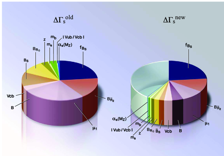
Figure 3: Uncertainty budget for the theory prediction of $\Delta\Gamma_{s}$. The largest uncertainties stem from $f_{B_{s}}$, the renormalisation scale $\mu_{1}$ of the $\Delta B=1$ operators and the bag parameter of the $1/m_{b}$–suppressed operator $\widetilde{R}_{2}$. The transparent segment of the right pie chart shows the improvement with respect to the old result on the left.

 

In the case of $\Delta\Gamma_{s}$ the by far largest uncertainty stems from the error on $f_{B_{s}}$. Here a considerable improvement from the non-perturbative side is mandatory. The dependence on the decay constant is of course not affected by the change of the operator basis. The second most important uncertainty comes from the $1/m_{b}$-operator $\tilde{R}_{2}$. This operator has up to now only been estimated in the naive vacuum insertion approximation. Any non-perturbative investigation would be very helpful. Number three in the error hit list is the unphysical $\mu_{1}$-dependence. Using the old operator basis the corresponding error was huge, it was drastically reduced by changing to the new basis and by including also the $\overline{\mbox{MS}}$-scheme for the b-quark mass. Any further improvement requires a cumbersome NNLO calculation, which might be worthwhile if progress on the non-perturbative side for $f_{B_{s}}$ and $\tilde{R}_{2}$ is achieved. Number four is again a non-perturbative parameter - now the bag parameter of the operator $Q$. In the old operator basis the corresponding uncertainty stemmed from $B_{S}$ and was larger by a factor of 2.5. The dependence on $V_{cb}$ results in a relative error of about $5\%$ for both the old basis and the new basis. All remaining uncertainties are at most $3\%$.
Using our conservative estimates and adding all errors quadratically (after symmetrising them) we arrive at a reduction of the overall theoretical error due to the introduction of the new basis from $\pm 61\%$ to $\pm 41\%$, where the last number is completely dominated by the decay constant. If one neglects the dependence on $f_{B_{s}}$ the overall theoretical error goes down from $\pm 51\%$ to $\pm 23\%$.
In the table in Eq. (63) we also show the dependence on the b-quark mass we are using in the $1/m_{b}$-corrections, $m_{b}^{\rm pow}$. This dependence can be viewed as a measure of the overall size of the $1/m_{b}$-corrections. The use of the new basis results in a strong reduction of the corresponding uncertainty, from $37\%$ to $11\%$. And finally we compare the two renormalisation schemes (RS) we are using for the b-quark mass. Here we have again muss less uncertainty in the new operator basis. To avoid a double counting of the errors we did not include the last two rows of table (63) in the total error.
Investigating the case of $\Delta\Gamma_{s}/\Delta M_{s}$ the improvement due to our new basis is more substantial, since here the dependence on $f_{B_{s}}$ cancels:

$\begin{array}[]{|c||c|c||c|}\hline\cr\mbox{Input}&\Delta\Gamma_{s}/\Delta M_{s}&\Delta\Gamma_{s}/\Delta M_{s}&a_{\rm fs}^{s}\\ &\mbox{old, pole, z}&\mbox{new, average, }\overline{z}&\mbox{new, average, }\overline{z}\\ \hline\cr\hline\cr B_{1}&1^{+0.074}_{-0.064}&1\pm 0.005&1^{+0.006}_{-0.005}\\ \hline\cr B_{2,3}&1\pm 0.167&1\pm 0.031&1\pm 0.004\\ \hline\cr B_{\tilde{R}_{2}}&1\pm 0.235&1\pm 0.157&1\pm 0.025(\tilde{R}_{3})\\ \hline\cr B_{R_{0}}&1\pm 0.140&1\pm 0.030&1\pm 0.011(R_{3})\\ \hline\cr\mu_{1}\mbox{ with }m_{b}/2\leq\mu_{1}\leq 2m_{b}&1^{+0.194}_{-0.495}&1^{+0.027}_{-0.154}&1^{+0.152}_{-0.101}\\ \hline\cr V_{cb}&1\pm 0.000&1\pm 0.000&1\pm 0.000\\ \hline\cr z&1^{+0.044}_{-0.046}&1\pm 0.019&1^{+0.094}_{-0.092}\\ \hline\cr m_{b}&1^{+0.043}_{-0.042}&1^{+0.010}_{-0.009}&1^{+0.037}_{-0.036}\\ \hline\cr m_{t}&1\pm 0.018&1\pm 0.018&1\pm 0.018\\ \hline\cr\alpha_{s}&1\pm 0.012&1\pm 0.001&1\pm 0.007\\ \hline\cr m_{s}&1\pm 0.010&1\pm 0.010&1\pm 0.001\\ \hline\cr\gamma&1^{+0.001}_{-0.003}&1^{+0.000}_{-0.001}&1^{+0.144}_{-0.081}\\ \hline\cr|V_{ub}/V_{cb}|&1\pm 0.001&1\pm 0.001&1^{+0.194}_{-0.196}\\ \hline\cr\hline\cr\sqrt{\sum\bar{\delta}^{2}}&1\pm 0.480&1\pm 0.189&1\pm 0.279\\ \hline\cr\hline\cr m_{b}^{\rm pow}&1_{-0.368}&1_{-0.112}&1^{+0.016}\\ \hline\cr\mbox{RS}&1\pm 0.136&1\pm 0.069&1\pm 0.004\\ \hline\cr\end{array}$

 

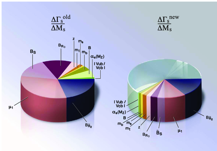
Figure 4: Uncertainty budget for $\Delta\Gamma_{s}/\Delta M_{s}$. See Fig. 3 for explanations. The ratio $\Delta\Gamma_{s}/\Delta M_{s}$ does not depend on $f_{B_{s}}$ and the progress due to the new operator basis is more substantial than in $\Delta\Gamma_{s}$.

 

In the case of $\Delta\Gamma_{s}/\Delta M_{s}$ the use of the new operator basis leads to a reduction of the total error from $48\%$ to $19\%$! The dominant error is now due to the bag parameter $B_{\tilde{R}_{2}}$, followed by the $\mu_{1}$-dependence. The remaining uncertainties are at most $3\%$. In the case of $a_{\rm fs}^{s}$ the situation is quite different. Here the dominant uncertainty stems from $V_{ub}$, followed by the dependences on $\mu_{1}$, $\gamma$ and $\overline{z}$. Moreover the $1/m_{b}$-corrections play a minor role here — as can be read off from the error due to the variation of $m_{b}^{\rm pow}$.

3.4 $\Delta M_{d}$, $\Delta\Gamma_{d}$ and $a_{\rm fs}^{d}$ within the SM

Here we give updated numbers for the mixing parameters of the $B_{d}$ system. The CKM elements governing $B_{d}\!-\!\,\overline{\!B}{}_{d}\,$ mixing appear in the combinations $\lambda_{i}^{d}=V_{id}^{*}V_{ib}$ for $i=u,c,t$. The bag parameters multiplying $f_{B_{d}}$ below refer to $B_{d}$ mesons and are different from those in the $B_{s}$ system. However, no non-perturbative computation has shown any numerically relevant deviation of $B_{B_{d}}/B_{B_{s}}$ from 1.

Updating $\Delta M_{d}$ to $\overline{m}_{t}(\overline{m}_{t})=163.8\pm 2.0\,{\rm GeV}$ gives

$$\Delta M_{d}=(0.53\pm 0.02)\,\mbox{ps}^{-1}{\left(\frac{|V_{td}|}{0.0082}\right)^{2}}\;\left(\frac{f_{B_{d}}}{200\,\mbox{MeV}}\right)^{2}\frac{B}{0.85}.$$

While in the $B_{s}$ system the values of $\gamma$ and $|V_{ub}|$ in Eq. (37) play a minor role, their uncertainties are an issue for $\Delta\Gamma_{d}$ and $a_{\rm fs}^{d}$. The master formulae are [21]

$$\frac{\Delta\Gamma_{d}}{\Delta M_{d}} = -\,10^{-4}\left[c\;+\;a\,\mathrm{Re}\,\frac{\lambda_{u}^{d}}{\lambda_{t}^{d}}\;+\;b\,\mathrm{Re}\,\frac{\lambda_{u}^{d\,2}}{\lambda_{t}^{d\,2}}\right]$$ (64)

$$a_{\rm fs}^{d} = 10^{-4}\left[a\,\mathrm{Im}\,\frac{\lambda_{u}^{d}}{\lambda_{t}^{d}}\;+\;b\,\mathrm{Im}\,\frac{\lambda_{u}^{d\,2}}{\lambda_{t}^{d\,2}}\right].$$ (65)

The coefficients

$$\qquad a = 2\cdot 10^{4}\,\frac{\Gamma_{12}^{uc}-\Gamma_{12}^{cc}}{M_{12}^{d}/\lambda_{t}^{d\,2}},\qquad b\;=\;10^{4}\,\frac{2\Gamma_{12}^{uc}-\Gamma_{12}^{cc}-\Gamma_{12}^{uu}}{M_{12}^{d}/\lambda_{t}^{d\,2}}$$

$$\mbox{and }\quad c = -10^{4}\,\frac{\Gamma_{12}^{cc}}{M_{12}^{d}/\lambda_{t}^{d\,2}}$$ (66)

are independent of CKM elements because of $M_{12}^{d}\propto\lambda_{t}^{d\,2}$. In our new operator basis these coefficients read

$$a = 9.68\raisebox{-2.15277pt}{\shortstack[l]{$\scriptstyle+1.53$\\ $\scriptstyle-1.48$}}\;+\;\left(0.31\raisebox{-2.15277pt}{\shortstack[l]{$\scriptstyle+0.09$\\ $\scriptstyle-0.07$}}\right)\frac{\widetilde{B}_{S}^{\prime}}{B}\;+\;\left(0.27\raisebox{-2.15277pt}{\shortstack[l]{$\scriptstyle+0.15$\\ $\scriptstyle-0.06$}}\right)\frac{B_{R}}{B}$$

$$b = 0.08\pm 0.03\;+\;\left(0.02\pm 0.01\right)\frac{\widetilde{B}_{S}^{\prime}}{B}\;+\;\left(0.04\raisebox{-2.15277pt}{\shortstack[l]{$\scriptstyle+0.03$\\ $\scriptstyle-0.01$}}\right)\frac{B_{R}}{B}$$

$$c = -46.1\pm 6.6\;-\;\left(10.5\pm 1.3\right)\frac{\widetilde{B}_{S}^{\prime}}{B}\;+\;\left(8.7\raisebox{-2.15277pt}{\shortstack[l]{$\scriptstyle+4.9$\\ $\scriptstyle-1.0$}}\right)\frac{B_{R}}{B}.$$

With the hadronic parameters of Set I in Eq. (39) one finds

$$a = 10.5\raisebox{-2.15277pt}{\shortstack[l]{$\scriptstyle+1.8$\\ $\scriptstyle-1.7$}},\qquad b\;=\;0.2\pm 0.1,\qquad c\;=\;-53.3\raisebox{-2.15277pt}{\shortstack[l]{$\scriptstyle+12.7$\\ $\scriptstyle-11.4$}}$$ (67)

It is convenient to express $\lambda_{u}^{d}/\lambda_{t}^{d}$ in Eqs. (64) and (65) in terms of the angle $\beta=\arg(-\lambda_{t}^{d}/\lambda_{c}^{d})$ of the unitarity triangle and the length $R_{t}=|\lambda_{t}^{d}/\lambda_{c}^{d}|$ of the adjacent side [21]:

$$\mathrm{Re}\,\frac{\lambda_{u}^{d}}{\lambda_{t}^{d}} = \frac{\cos\beta}{R_{t}}-1,\qquad\mathrm{Re}\,\frac{\lambda_{u}^{d\,2}}{\lambda_{t}^{d\,2}}\;=\;\frac{\cos(2\beta)}{R_{t}^{2}}-2\frac{\cos\beta}{R_{t}}+1,$$

$$\mathrm{Im}\,\frac{\lambda_{u}^{d}}{\lambda_{t}^{d}} = -\frac{\sin\beta}{R_{t}},\qquad\mathrm{Im}\,\frac{\lambda_{u}^{d\,2}}{\lambda_{t}^{d\,2}}\;=\;-\frac{\sin(2\beta)}{R_{t}^{2}}+2\frac{\sin\beta}{R_{t}}.$$ (68)

Clearly the terms involving $\lambda_{u}^{d\,2}/\lambda_{t}^{d\,2}$ in Eqs. (64) and (65) are numerically irrelevant in view of the smallness of $b$. Moreover, in the preferred region of the Standard Model fit of the unitarity triangle one has $\cos\beta\approx R_{t}$, so that $\mathrm{Re}\,\lambda_{u}^{d}/\lambda_{t}^{d}$ is suppressed. Setting $a$ and $b$ to zero in Eq. (64) reproduces $\Delta\Gamma_{d}/\Delta M_{d}$ within 2% [21] and $\Delta\Gamma_{d}/\Delta M_{d}$ is essentially free of CKM uncertainties.

Inserting Eqs. (67) and (68) into Eqs. (64) and (65) yields

$$\frac{\Delta\Gamma_{d}}{\Delta M_{d}} = \left[53.3\raisebox{-2.15277pt}{\shortstack[l]{$\scriptstyle+11.4$\\ $\scriptstyle-12.7$}}\;+\;\left(10.3\raisebox{-2.15277pt}{\shortstack[l]{$\scriptstyle+1.8$\\ $\scriptstyle-1.7$}}\right)\,\left(1\,-\,\frac{\cos(\beta)}{R_{t}}\right)\right.$$ (69)

$$\left.\qquad\qquad\;+\;(0.2\pm 0.1)\,\left(\frac{\cos(\beta)}{R_{t}}-\frac{\cos(2\beta)}{R_{t}^{2}}\right)\right]\cdot 10^{-4}$$

$$a_{\rm fs}^{d} = -\left[\left(10.1\raisebox{-2.15277pt}{\shortstack[l]{$\scriptstyle+1.8$\\ $\scriptstyle-1.7$}}\right)\,\frac{\sin\beta}{R_{t}}\;+\;(0.2\pm 0.1)\,\frac{\sin(2\beta)}{R_{t}^{2}}\right]\cdot 10^{-4}$$ (70)

Next we insert the numerical values for $\beta$ and $R_{t}$ from [2]. Since we are interested in testing the hypothesis of new physics in $B_{s}\!-\!\,\overline{\!B}{}_{s}\,$ mixing, we take values for $\beta$ and $R_{t}$ obtained prior to the measurement of $\Delta M_{s}$. With $\beta=23^{\circ}\pm 2^{\circ}$ and $R_{t}=0.86\pm 0.11$, which correspond to a CL of 2$\sigma$, one finds

$$\frac{\Delta\Gamma_{d}}{\Delta M_{d}} = \left(52.6\raisebox{-2.15277pt}{\shortstack[l]{$\scriptstyle+11.5$\\ $\scriptstyle-12.8$}}\right)\,\cdot 10^{-4},\qquad\qquad a_{\rm fs}^{d}\;=\;\left(-4.8\raisebox{-2.15277pt}{\shortstack[l]{$\scriptstyle+1.0$\\ $\scriptstyle-1.2$}}\right)\,\cdot 10^{-4}.$$ (71)

Thus these predictions allow for new physics in $\Delta M_{s}$, but assume that all other quantities entering the standard fit of the unitarity triangle in [2] are as in the Standard Model. Using $\Delta M_{d}^{\rm exp}=0.507\pm 0.004\,{\rm ps}^{-1}$ and $\tau_{B_{d}}^{\rm exp}=1.530\pm 0.009$ we find from Eq. (71):

$$\Delta\Gamma_{d} = \frac{\Delta\Gamma_{d}}{\Delta M_{d}}\,\Delta M_{d}^{\rm exp}\;=\;\left(26.7\raisebox{-2.15277pt}{\shortstack[l]{$\scriptstyle+5.8$\\ $\scriptstyle-6.5$}}\right)\cdot 10^{-4}\;{\rm ps}^{-1},\qquad\frac{\Delta\Gamma_{d}}{\Gamma_{d}}\;=\;\left(40.9\raisebox{-2.15277pt}{\shortstack[l]{$\scriptstyle+8.9$\\ $\scriptstyle-9.9$}}\right)\cdot 10^{-4}.$$ (72)

The result in Eq. (72) is consistent with our prediction in [21], but the central value is substantially higher. This is not solely caused by our new operator basis, but also by the use of a different renormalisation scheme. In both [21] and this work we average over two schemes, but in one of the schemes used in [21] the $z\ln z$ terms are not summed to all orders. Note that the quoted error of $a_{\rm fs}^{d}$ in [21] corresponds to the 1$\sigma$ ranges of $\beta$ and $R_{t}$, while in Eq. (71) more conservative 2$\sigma$ intervals have been used. The ranges in Eq. (71) imply for the CP-violating phase $\phi_{d}=\arg(-M_{12}^{d}/\Gamma_{12}^{d})$:

$$\phi_{d} = -0.091\raisebox{-2.15277pt}{\shortstack[l]{$\scriptstyle+0.026$\\ $\scriptstyle-0.038$}}\;=\;-5.2^{\circ}\raisebox{-2.15277pt}{\shortstack[l]{$\scriptstyle+1.5^{\circ}$\\ $\scriptstyle-2.1^{\circ}$}}\,.$$ (73)

4 Constraining new physics with $B_{s}\!-\!\,\overline{\!B}{}_{s}\,$ mixing

In this section we investigate effects of new physics contributions to the $B_{s}$-mixing parameters. New physics can change the magnitude and the phase of $M_{12}^{s}$. We parameterise its effect (similarly to [42, 2]) by

$$M_{12}^{s} \equiv M_{12}^{\rm SM,s}\cdot\Delta_{s}\,,\qquad\qquad\Delta_{s}\;\equiv\;|\Delta_{s}|e^{i\phi^{\Delta}_{s}}.$$ (74)

The relationship to the parameters used in [14, 2] is

$$\Delta_{s} = r_{s}^{2}e^{2i\theta_{s}}.$$

We find it more transparent to plot $\mathrm{Im}\,\Delta_{s}$ vs. $\mathrm{Re}\,\Delta_{s}$ than to plot $2\theta_{s}$ vs. $r_{s}^{2}$. Our plots are similar to Fig. 1 of [14], which displays $\sin(2\theta_{s})$ vs. $\cos(2\theta_{s})$, but also include the information on $|\Delta_{s}|\equiv r_{s}^{2}$. Finally $\Gamma_{12}^{s}$ stems from CKM-favoured tree decays and one can safely set $\Gamma_{12}^{s}=\Gamma_{12}^{\rm SM,s}$.

4.1 $\Delta\Gamma_{s}$, $\Delta\Gamma_{s}/\Delta M_{s}$ and $a_{\rm fs}^{s}$ beyond the SM

One easily finds:

$$\Delta M_{s} = \Delta M_{s}^{\rm SM}\,|\Delta_{s}|=(19.30\pm 6.74)\,\mbox{ps}^{-1}\cdot|\Delta_{s}|$$ (75)

$$\Delta\Gamma_{s} = 2|\Gamma_{12}^{s}|\,\cos\left(\phi_{s}^{\rm SM}+\phi^{\Delta}_{s}\right)=(0.096\pm 0.039)\,\mbox{ps}^{-1}\cdot\cos\left(\phi_{s}^{\rm SM}+\phi^{\Delta}_{s}\right)$$ (76)

$$\frac{\Delta\Gamma_{s}}{\Delta M_{s}} = \frac{|\Gamma_{12}^{s}|}{|M_{12}^{\rm SM,s}|}\cdot\frac{\cos\left(\phi_{s}^{\rm SM}+\phi^{\Delta}_{s}\right)}{|\Delta_{s}|}=\left(4.97\pm 0.94\right)\cdot 10^{-3}\cdot\frac{\cos\left(\phi_{s}^{\rm SM}+\phi^{\Delta}_{s}\right)}{|\Delta_{s}|}$$ (77)

$$a_{\rm fs}^{s} = \frac{|\Gamma_{12}^{s}|}{|M_{12}^{\rm SM,s}|}\cdot\frac{\sin\left(\phi_{s}^{\rm SM}+\phi^{\Delta}_{s}\right)}{|\Delta_{s}|}=\left(4.97\pm 0.94\right)\cdot 10^{-3}\cdot\frac{\sin\left(\phi_{s}^{\rm SM}+\phi^{\Delta}_{s}\right)}{|\Delta_{s}|}$$ (78)

$$\mbox{with (cf.\ Eq.~{}(\ref{finphi}))}\qquad\phi_{s}^{\rm SM}=(4.2\pm 1.4)\cdot 10^{-3}$$ . (79)

Here the numerical values correspond to our results from parameter set I in Eqs. (54–57). In the case of $a_{\rm fs}^{s}$ there is a major difference to the SM case of Sect. 3.3, which only involves $\mathrm{Im}\,(\Gamma_{12}^{s}/M_{12}^{s})$: in the presence of new physics $a_{\rm fs}^{s}$ is dominated by $\mathrm{Re}\,(\Gamma_{12}^{s}/M_{12}^{s})$ as long as $|\phi^{\Delta}_{s}|>\phi_{s}^{\rm SM}$. Thus the prediction in Eq. (78) profits from the improvements due to our new operator basis — just as the prediction of $\Delta\Gamma_{s}$ in Eq. (77). From Eq. (78) one also verifies the enormous sensitivity of $a_{\rm fs}^{s}$ to new physics, since it exceeds its SM value by a factor of 250 for $\phi^{\Delta}_{s}=\pi/2$. We have plotted $a_{\rm fs}^{s}$ vs. $\phi^{\Delta}_{s}$ for the old and the new bases in Fig. 5.

 

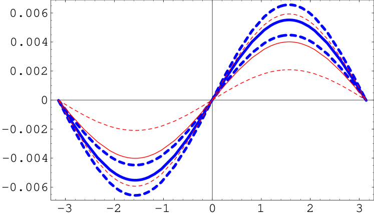
Figure 5: $a_{\rm fs}^{s}$ as a function of the new phase $\phi^{\Delta}_{s}$ from Eq. (78) for the range $-\pi\leq\phi^{\Delta}_{s}\leq\pi$. The thick blue lines show the prediction in the new basis, while thin red lines correspond to the old operator basis. The solid lines display the central values of our predictions and the dashed lines show the uncertainties, which are much larger for the old result. The standard model value $a_{\rm fs}^{s}(\phi^{\Delta}_{s}=0)=2.1\cdot 10^{-5}$ is too close to zero to be visible in the plot.

 

4.2 Basic observables

In this section we summarise the observables which constrain $|\Delta_{s}|$ and $\phi^{\Delta}_{s}$. These constraints are illustrated in Fig. 6 for hypothetical measurements.

1. The mass difference $\Delta M_{s}$ determines $|\Delta_{s}|$ through Eq. (75). The accuracy of $|\Delta_{s}|$ extracted from $\Delta M_{s}$ is limited by the precision of a lattice computation. This is not the case for the other quantities discussed in this section.

Alternatively one can confront the experimental ratio $\Delta M_{d}/\Delta M_{s}$ with theory. This has the advantage that the ratio of the hadronic matrix elements involved can be predicted with a smaller error, of order 5%. However, then the parameter of $R_{t}$ of the unitarity triangle entering $\Delta M_{d}$ must be taken from measurements which are insensitive to new physics (or at least insensitive to new physics in $B_{s}\!-\!\,\overline{\!B}{}_{s}\,$ mixing), e.g. through determinations of the CKM angle $\gamma$ from tree-level B decays (cf. the discussion after Eq. (70)). At present this method leads to comparable uncertainties in the extracted $|\Delta_{s}|$ as the direct determination from $\Delta M_{s}$. (Further flavour-blind new physics cancels from $\Delta M_{d}/\Delta M_{s}$.) In the following analyses we do not use $\Delta M_{d}/\Delta M_{s}$.

2. The lifetime measurement in an untagged $b\to c\overline{c}s$ decay $\raisebox{7.7pt}{$\scriptscriptstyle(\hskip 8.5pt)$}\!\,\overline{\!B}_{s}\to f_{CP}$, where $f_{CP}$ is a CP eigenstate, determines $\Delta\Gamma_{s}\cos(\phi_{s}^{\Delta}-2\beta_{s})=|\Delta\Gamma_{s}\cos(\phi_{s}^{\Delta}-2\beta_{s})|$ [43, 44]. Consider a CP-even final state $f_{CP+}$ like $D_{s}^{+}D_{s}^{-}$. The time-dependent decay rate reads

$$\Gamma[\raisebox{7.7pt}{$\scriptscriptstyle(\hskip 8.5pt)$}\!\,\overline{\!B}_{s}\to f_{CP+},t]\propto\frac{1+\cos(\phi_{s}^{\Delta}-2\beta_{s})}{2}e^{-\Gamma_{L}t}\;+\>\frac{1-\cos(\phi_{s}^{\Delta}-2\beta_{s})}{2}e^{-\Gamma_{H}t}$$

$$\;=\;e^{-\Gamma_{s}t}\left[\cosh\frac{\Delta\Gamma_{s}\,t}{2}-\cos(\phi_{s}^{\Delta}-2\beta_{s})\sinh\frac{\Delta\Gamma_{s}\,t}{2}\right]$$ (80)

and the (time-independent) overall normalisation is related to the branching fraction [44]. Here

$$\beta_{s} = -\arg\left(-\frac{\lambda_{t}^{s}}{\lambda_{c}^{s}}\right)\;=\;0.020\pm 0.005\;=\;1.1^{\circ}\pm 0.3^{\circ}.$$ (81)

That is, $-\beta_{s}$ is the analogue of the angle $\beta$ of the unitarity triangle, which governs the mixing-induced CP asymmetry in $B_{d}\to J/\psi K_{S}$, in the $B_{s}$ system. For $\beta_{s}$ different sign conventions are used in the literature, we chose the one of [6] which satisfies $\beta_{s}>0$.

For example within the Standard Model (and neglecting the tiny $\beta_{s}$) the lifetime measured in $\raisebox{7.7pt}{$\scriptscriptstyle(\hskip 8.5pt)$}\!\,\overline{\!B}_{s}\to D_{s}^{+}D_{s}^{-}$ equals $\Gamma^{s}_{L}=\Gamma_{s}+\Delta\Gamma/2$, because only the short-lived CP-even mass eigenstate $B_{L}$ can decay into $D_{s}^{+}D_{s}^{-}$. By using the theory relation $1/\tau_{B_{d}}=\Gamma_{d}=(1.00\pm 0.01)\Gamma_{s}$ one then finds $\Delta\Gamma_{s}$. For $\phi_{s}^{\Delta}\neq 0$, however, the mass eigenstates are no more CP eigenstates and both of them can decay to a CP eigenstate, as can be easily verified from Eq. (80). From $\Gamma[\raisebox{7.7pt}{$\scriptscriptstyle(\hskip 8.5pt)$}\!\,\overline{\!B}_{s}\to f_{CP+},t]$ one can extract $|\Gamma_{s}|$, $|\Delta\Gamma_{s}|$, $|\cos(\phi_{s}^{\Delta})|$ and the overall normalisation, if the statistics is high enough to separate the two exponentials. If the measured $\Gamma[\raisebox{7.7pt}{$\scriptscriptstyle(\hskip 8.5pt)$}\!\,\overline{\!B}_{s}\to f_{CP+},t]$ is fitted to a single exponential $\exp[-\Gamma_{f}\,t]$, the measured rate is [45, 44]

$$\Gamma_{f} = \frac{(1+\cos(\phi_{s}^{\Delta}-2\beta_{s}))/\Gamma_{L}+(1-\cos(\phi_{s}^{\Delta}-2\beta_{s}))/\Gamma_{H}}{(1+\cos(\phi_{s}^{\Delta}-2\beta_{s}))/\Gamma_{L}^{2}+(1-\cos(\phi_{s}^{\Delta}-2\beta_{s}))/\Gamma_{H}^{2}}$$

$$= \Gamma_{s}\;+\;\Delta\Gamma_{s}\cos(\phi_{s}^{\Delta}-2\beta_{s})\;+\>{\cal O}\left(\frac{(\Delta\Gamma_{s})^{2}}{\Gamma_{s}}\right)$$

$$= \Gamma_{s}\;+\;2\,|\Gamma_{12}^{s}|\cos(\phi_{s}^{\Delta}+\phi_{s}^{\rm SM})\cos(\phi_{s}^{\Delta}-2\beta_{s})\;+\>{\cal O}\left(\frac{(\Delta\Gamma_{s})^{2}}{\Gamma_{s}}\right).$$ (83)

For a CP-odd final state one has to interchange $\Gamma_{L}$ and $\Gamma_{H}$ in Eqs. (80) and (4.2) and to flip the sign of $\cos(\phi_{s}^{\Delta}-2\beta_{s})$ in Eqs. (80) and (83). From Eq. (83) it is clear that the lifetime measurement determines [43, 44]

$$\Delta\Gamma_{s}\cos(\phi_{s}^{\Delta}) = 2|\Gamma_{12}^{s}|\cos^{2}(\phi_{s}^{\Delta}),$$

if the small phases $\phi_{s}^{\rm SM}$ and $\beta_{s}$ are neglected. Thus one can find $|\cos\phi_{s}^{\Delta}|$, which determines $\phi_{s}^{\Delta}$ with a four-fold ambiguity. We stress that (since $\mbox{sign}\,\Delta\Gamma_{s}=\mbox{sign}\,\cos(\phi_{s}^{\Delta})$) the lifetime method gives no information on the sign of $\Delta\Gamma_{s}$ and experimental results should be quoted for $|\Delta\Gamma_{s}|$ rather than $\Delta\Gamma_{s}$.

Eq. (4.2) assumes that detection efficiencies are constant over the decay time. Since this is not the case in real experiments, we strongly recommend to perform a three-parameter fit to $2|\Gamma_{12}|$, $|\cos(\phi_{s}^{\Delta})|$ and the overall normalisation (with $|\Gamma_{s}|$ fixed to $|\Gamma_{d}|(1.00\pm 0.01)$) to Eq. (80).

With the advent of the precise measurement of $\Delta M_{s}$ [10] one will rather exploit $|\Delta\Gamma_{s}|/\Delta M_{s}$ to constrain $\Delta_{s}$ than $|\Delta\Gamma_{s}|$ itself, which suffers from much larger hadronic uncertainties. From Eq. (77) one infers that $|\Delta\Gamma_{s}|/\Delta M_{s}$ defines two circles in the complex $\Delta_{s}$ plane which touch the y–axis at the origin.

3. The angular analysis of an untagged $b\to c\overline{c}s$ decay $\raisebox{7.7pt}{$\scriptscriptstyle(\hskip 8.5pt)$}\!\,\overline{\!B}_{s}\to VV^{\prime}$, where $VV^{\prime}$ is a superposition of CP eigenstates with vector mesons $V,V^{\prime}$, not only determines $\Delta\Gamma_{s}\cos(\phi_{s}^{\Delta}-2\beta_{s})$, but also contains information on $\sin(\phi_{s}^{\Delta}-2\beta_{s})$ through a CP-odd interference term. Here the golden mode is certainly $\raisebox{7.7pt}{$\scriptscriptstyle(\hskip 8.5pt)$}\!\,\overline{\!B}_{s}\to J/\psi\phi$, but also final states with higher $\psi$ resonances and $\raisebox{7.7pt}{$\scriptscriptstyle(\hskip 8.5pt)$}\!\,\overline{\!B}_{s}\to D_{s}^{*+}D_{s}^{*-}$ can be studied. The determination of $\phi_{s}^{\Delta}$ from the CP-odd interference term in untagged samples involves a four-fold ambiguity. It could be reduced to a two-fold ambiguity if the signs of $\cos\delta_{1}$ and $\cos\delta_{2}$ were determined, where $\delta_{1}$ and $\delta_{2}$ are the strong phases involved [46, 44]. These two solution are related by $\phi_{s}^{\Delta}\leftrightarrow\phi_{s}^{\Delta}\pm\pi$. If one relaxes the assumptions on $\cos\delta_{1}$ and $\cos\delta_{2}$, one is back to the same four-fold ambiguity as in item 2.

4.  The branching fraction $Br(\raisebox{7.7pt}{$\scriptscriptstyle(\hskip 8.5pt)$}\!\,\overline{\!B}_{s}\to D_{s}^{(*)+}D_{s}^{(*)-})$ approximates the width difference $\Delta\Gamma_{\rm CP}$ between the two CP eigenstates of the $B_{s}$ system [44]. Irrespective of any new physics in $M_{12}^{s}$ one always has $\Delta\Gamma_{\rm CP}=2|\Gamma_{12}^{s}|$, so no constraint on our new physics parameter $\Delta_{s}$ is gained. Yet the ratio of $\Delta\Gamma_{s}\cos(\phi_{s}^{\Delta}-2\beta_{s})$ and $\Delta\Gamma_{\rm CP}$ could cleanly determine $\cos(\phi_{s}^{\Delta})\cos(\phi_{s}^{\Delta}-2\beta_{s})$. However, $Br(\raisebox{7.7pt}{$\scriptscriptstyle(\hskip 8.5pt)$}\!\,\overline{\!B}_{s}\to D_{s}^{(*)+}D_{s}^{(*)-})$ only equals $\Delta\Gamma_{\rm CP}$ in the poorly tested simultaneous limit of an infinitely heavy charm quark with small-velocity [47] and an infinite number of colours [48]. In order to test this limit one needs to measure the CP-odd and CP-even fractions of all $b\to c\overline{c}s$ decays [44]. Until this has been done nothing can be inferred from $Br(\raisebox{7.7pt}{$\scriptscriptstyle(\hskip 8.5pt)$}\!\,\overline{\!B}_{s}\to D_{s}^{(*)+}D_{s}^{(*)-})$, in particular this quantity neither gives an upper bound (since other CP-even $b\to c\overline{c}s$ modes can be relevant) nor a lower bound (since other CP-odd $b\to c\overline{c}s$ modes can be relevant and the $D_{s}^{(*)+}D_{s}^{(*)-}$ final state has a CP-odd component) on $\Delta\Gamma_{\rm CP}$. We strongly discourage from the inclusion of $Br(\raisebox{7.7pt}{$\scriptscriptstyle(\hskip 8.5pt)$}\!\,\overline{\!B}_{s}\to D_{s}^{(*)+}D_{s}^{(*)-})$ in averages with $\Delta\Gamma_{s}$ determined from clean methods.

5. $a_{\rm fs}^{s}$ can be measured from untagged flavour-specific $\raisebox{7.7pt}{$\scriptscriptstyle(\hskip 8.5pt)$}\!\,\overline{\!B}_{s}$ decays, typically from the number of positively and negatively charged leptons in semileptonic decays. Observing further the time evolution of these untagged $\raisebox{7.7pt}{$\scriptscriptstyle(\hskip 8.5pt)$}\!\,\overline{\!B}_{s}\to X^{\mp}\ell^{\pm}\,\raisebox{5.5pt}{$\scriptscriptstyle(\hskip 6.3pt)$}\!\overline{\nu}_{\ell}$ decays (see e.g. [8]),

$$\frac{\Gamma[\raisebox{7.7pt}{$\scriptscriptstyle(\hskip 8.5pt)$}\!\,\overline{\!B}_{s}\to X^{-}\ell^{+}\nu_{\ell},t]\,-\,\Gamma[\raisebox{7.7pt}{$\scriptscriptstyle(\hskip 8.5pt)$}\!\,\overline{\!B}_{s}\to X^{+}\ell^{-}\overline{\nu}_{\ell},t]}{\Gamma[\raisebox{7.7pt}{$\scriptscriptstyle(\hskip 8.5pt)$}\!\,\overline{\!B}_{s}\to X^{-}\ell^{+}\nu_{\ell},t]\,+\,\Gamma[\raisebox{7.7pt}{$\scriptscriptstyle(\hskip 8.5pt)$}\!\,\overline{\!B}_{s}\to X^{+}\ell^{-}\overline{\nu}_{\ell},t]} = \frac{a_{\rm fs}^{s}}{2}\left[1-\frac{\cos(\Delta M_{s}\,t)}{\cosh{(\Delta\Gamma_{s}\,t/2)}}\right],$$ (84)

will have two advantages: one can use the oscillatory behaviour to control fake effects from experimental detection asymmetries (which are constant in time) and to separate the $B_{s}$ and $B_{d}$ samples through $\Delta M_{s}\neq\Delta M_{d}$. The constraint from $a_{\rm fs}^{s}$ on $\Delta_{s}$ is given in Eq. (78). It defines a circle in the complex $\Delta_{s}$ plane which touches the x–axis at the origin. The constraint from $a_{\rm fs}^{s}$ on $\Delta_{s}$ only has a two-fold ambiguity (related to $\phi_{s}\leftrightarrow\pi-\phi_{s}$) and discriminates between the solutions in the upper and lower half–plane in Fig. 6.

6. The time dependence of the tagged decay $B_{s}\to J/\psi\phi$ permits the determination of the mixing-induced CP asymmetries $A_{\rm CP}^{\rm mix}(B_{s}\to(J/\psi\phi)_{CP\pm})$. The angular analysis separates the CP–odd P-wave component from the CP–even S-wave and D-wave. The time-dependent CP asymmetry is (in the notation of [6, 44]):

$$\frac{\Gamma(\bar{B}^{0}_{s}(t)\to f)-\Gamma(B^{0}_{s}(t)\to f)}{\Gamma(\bar{B}^{0}_{s}(t)\to f)+\Gamma(B^{0}_{s}(t)\to f)} = -\frac{A_{CP}^{\rm mix}\sin(\Delta M_{s}t)}{\cosh(\Delta\Gamma_{s}t/2)+A_{\Delta\Gamma}\sinh(\Delta\Gamma_{s}t/2)}.$$ (85)

One finds $\phi_{s}^{\Delta}-2\beta_{s}$ through

$$A_{\rm CP}^{\rm mix}(B_{s}\to(J/\psi\phi)_{CP\pm}) = \pm\sin(\phi_{s}^{\Delta}-2\beta_{s}),\qquad A_{\Delta\Gamma}\;=\;\mp\cos(\phi_{s}^{\Delta}-2\beta_{s})$$ (86)

with the same two-fold ambiguity as from $a_{\rm fs}^{s}$ in item 5. Combining Eqs. (75) and (78) with Eq. (86) and neglecting the tiny contributions of $\phi_{s}^{\rm SM}$ and $\beta_{s}$ one verifies the correlation between $a_{\rm fs}^{s}$ and $A_{\rm CP}^{\rm mix}(B_{s}\to(J/\psi\phi)_{CP\pm})$ derived in [12, 13]. In fact such correlations can be found between any three of the observables discussed above, because the $B_{s}\!-\!\,\overline{\!B}{}_{s}\,$ mixing only involves the two parameters $|\Delta_{s}|$ and $\phi_{s}$.

An important remark here concerns the decay $B_{s}\to K^{+}K^{-}$, as one might be tempted to use the lifetime measured in $B_{s}\to K^{+}K^{-}$ to determine $\Gamma_{s}+|\Delta\Gamma_{s}/2|$. While $K^{+}K^{-}$ is CP even, the decay is penguin–dominated and as such sensitive to the same kind of new physics which may be responsible for the experimental anomaly seen in penguin–dominated $B_{d}$ decays [3]. Thus information from $B_{s}\to K^{+}K^{-}$ should under no circumstances be included in any averages with the measurements discussed above. Instead one should confront the lifetime measured in this mode with the one obtained from $B_{s}\to(J/\psi\phi)_{CP+}$ to probe new physics in $b\to s$ penguin decays.

For a visualisation of the bounds from Eqs. (75–78) in the complex $\Delta_{s}$-plane we consider now the hypothetical case of $|\Delta_{s}|=0.9$ and $\phi^{\Delta}_{s}=-\pi/4$. Suppose one would measure these central values:

$$\Delta M_{s}=17.4\,\mbox{ps}^{-1}, \qquad\Delta\Gamma_{s}=0.068\,\mbox{ps}^{-1},$$ (87)

$$\frac{\Delta\Gamma_{s}}{\Delta M_{s}}=3.91\cdot 10^{-3}, \qquad a_{\rm fs}^{s}=-3.89\cdot 10^{-3}\,.$$ (88)

Moreover we assume the following theoretical and experimental uncertainties: $\Delta M_{s}:\pm 15\%$, $\Delta\phi_{s}:\pm 20\%$, $\Delta\Gamma_{s}/\Delta M_{s}:\pm 15\%$, $a_{\rm fs}^{s}:\pm 20\%$. The regions in the $\Delta_{s}$-plane bounded for these hypothetical measurements are shown in figure 6.

 

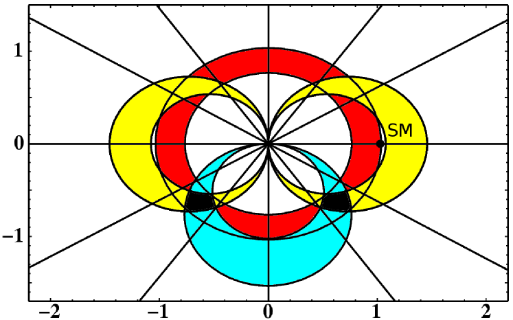
Figure 6: Illustration of the bounds in the complex $\Delta_{s}$-plane for $|\Delta_{s}|=0.9$ and $\phi^{\Delta}_{s}=-\pi/4$. We assume the following overall uncertainties: $\Delta M_{s}$ (red or dark-grey) : $\pm 15\%$, $\Delta\Gamma_{s}/\Delta M_{s}$ (yellow or light-grey): $\pm 15\%$, $a_{\rm fs}^{s}$ (light-blue or grey) : $\pm 20\%$ and $\phi_{s}^{\Delta}$ (solid lines) : $\pm 20\%$.

 

The constraints from CP-conserving quantities are symmetric to the Im($\Delta_{s}$)-axis, The bound from $\Delta M_{s}$ simply gives a circle with the origin (0,0) and the radius $|\Delta_{s}|$. In the measurement of $\Delta\Gamma_{s}$ we have assumed that the data are fitted to the correct formula Eq. (80) and $|\Delta\Gamma_{s}|$ and $|\cos(\phi_{s}-2\beta_{s})|$ have been determined as discussed above in item 2. In practice the extracted $|\Delta\Gamma_{s}|$ and $|\cos(\phi^{\Delta}_{s}-2\beta_{s})|$ are strongly correlated and mainly $|\Delta\Gamma_{s}||\cos(\phi^{\Delta}_{s}-2\beta_{s})|$ is determined (see Eq. (83) and [44]). The constraint from the hadronically cleaner ratio $|\Delta\Gamma_{s}|/\Delta M_{s}$ are two circles which touch the y–axis in the origin. If one fully includes the correlation between $|\Delta\Gamma_{s}|$ and $|\cos(\phi^{\Delta}_{s}-2\beta_{s})|$ one will rather find constraints which roughly correspond to a fixed $|\Delta\Gamma_{s}\cos(\phi^{\Delta}_{s}-2\beta_{s})|/\Delta M_{s}$. The corresponding curves are a bit more eccentric than the circles from $|\Delta\Gamma_{s}|/\Delta M_{s}$.

If one plots the bounds from $|\Delta\Gamma_{s}|$ (or $|\Delta\Gamma_{s}\cos(\phi^{\Delta}_{s}-2\beta_{s})|$) alone, one finds four rays starting from the origin. The experimental information in this is redundant, as it is fully contained in the constraints from $\Delta M_{s}$ and $|\Delta\Gamma_{s}|/\Delta M_{s}$. For the theory uncertainties, however, this is not true: if (as current data do) $\Delta M_{s}$ prefers a small value of $f_{B_{s}}$, while $\Delta\Gamma_{s}$ prefers a large $f_{B_{s}}$, the combined constraint from $\Delta M_{s}$ and $|\Delta\Gamma_{s}|$ will exclude a region of the $\Delta_{s}$ plane which is allowed by the ratio $|\Delta\Gamma_{s}|/\Delta M_{s}$, from which $f_{B_{s}}$ drops out.

The measurement of $a_{\rm fs}^{s}$ yields a circle touching the x–axis in the origin, in particular it reduces the four-fold ambiguity in the extracted value of $\Delta_{s}$ to a two-fold one. The extraction of $\phi^{\Delta}_{s}-2\beta_{s}$ from the angular analysis in $\raisebox{7.7pt}{$\scriptscriptstyle(\hskip 8.5pt)$}\!\,\overline{\!B}_{s}\to J/\psi\phi$ (as discussed in item 3) also yields four rays starting from the origin (corresponding to the same value of $|\cos(\phi^{\Delta}_{s}-2\beta_{s})|$), if no assumptions on the signs of $\cos\delta_{1}$ and $\cos\delta_{2}$ are made. Finally, the measurement of $A_{\rm CP}^{\rm mix}(B_{s}\to(J/\psi\phi)_{CP\pm})$ will select two out of these four rays, discriminating between $\phi_{s}^{\Delta}-2\beta_{s}>0$ and $\phi_{s}^{\Delta}-2\beta_{s}<0$.

4.3 Current experimental constraints on $\Delta_{s}$

In this section we turn to the real world and discuss the current experimental constraints on the complex $\Delta_{s}$-plane. In view of the experimental errors we set $\beta_{s}$ to zero and identify $\phi_{s}$ with $\phi^{\Delta}_{s}$.

The mass difference $\Delta M_{s}$ is now known very precisely [10], see Eq. (7). For the remaining mixing parameters in the $B_{s}$-system only weak experimental constraints are available. The only available experimental analysis of $|\Delta\Gamma_{s}|$ with the correct implementation of the phase $\phi_{s}$ is from the DØ collaboration, their analysis in [49] was recently updated in [50] using 1fb^-1 of data. Setting the value of the mixing phase $\phi_{s}$ to zero (Standard Model scenario) they obtain [50]

$$\Delta\Gamma_{s} = 0.12\pm 0.08{}_{\mbox{\scriptsize(stat)}}\;\raisebox{-2.15277pt}{\shortstack[l]{$\scriptstyle+0.03$\\ $\scriptstyle-0.04$}}\,{}_{\mbox{\scriptsize(syst)}}\;\mbox{ps}^{-1}\,.$$ (89)

Allowing for a non-zero value of the mixing phase $\phi_{s}$ they get

$$\Delta\Gamma_{s} = \phantom{-}0.17\pm 0.09{}_{\mbox{\scriptsize(stat)}}\;\pm 0.03{}_{\mbox{\scriptsize(syst)}}\;\mbox{ps}^{-1}\,$$ (90)

$$\mbox{and}\quad\phi_{s}\;=\;-0.79\pm 0.56{}_{\mbox{\scriptsize(stat)}}\pm 0.01{}_{\mbox{\scriptsize(syst)}}$$

$$\mbox{or}\qquad\Delta\Gamma_{s} = -0.17\pm 0.09{}_{\mbox{\scriptsize(stat)}}\pm 0.03{}_{\mbox{\scriptsize(syst)}}\,\mbox{ps}^{-1}\,$$ (91)

$$\mbox{and}\quad\phi_{s}\;=\;-0.79\pm 0.56{}_{\mbox{\scriptsize(stat)}}\pm 0.01{}_{\mbox{\scriptsize(syst)}}\;+\;\pi\,.$$

As expected from Eq. (83) the values for $|\Delta\Gamma_{s}\cos\phi_{s}|$ found from Eqs. (89) and (91) are roughly equal to $\Delta\Gamma_{s}$ in Eq. (89). The quoted results in Eqs. (90) and (91) assume that the signs of $\cos\delta_{1}$ and $\cos\delta_{2}$ agree with the results found with naive factorisation. With this assumption the other two solutions for $\phi_{s}$ (which have opposite signs to those in Eqs. (90) and (91)) are excluded. Strategies to check this theoretical input are discussed in [44].

The semileptonic CP asymmetry $a_{\rm sl}^{s}\equiv a_{\rm fs}^{s}$ in the $B_{s}$ system has been determined directly in [51] and was found to be

$$a_{\rm sl}^{s,\rm direct}=\left(24.5\pm 19.3{}_{\mbox{\scriptsize(stat)}}\pm 3.5{}_{\mbox{\scriptsize(syst)}}\right)\cdot 10^{-3}\,.$$ (92)

Moreover the semileptonic CP asymmetry can be extracted from the same sign dimuon asymmetry that was measured in [52] as

$$a_{\rm sl}=\left(-5.3\pm 2.5{}_{\mbox{\scriptsize(stat)}}\pm 1.8{}_{\mbox{\scriptsize(syst)}}\right)\cdot 10^{-3}\,$$ (93)

in a data sample containing both $B_{d}$ and $B_{s}$ mesons. While the composition of the sample is known, no determination of the initial state on an event–by–event basis was possible. Updating the numbers in [53, 14] one sees that the measurement in Eq. (93) determines the combination

$$a_{\rm sl}=\left(0.582\pm 0.030\right)\,a_{\rm sl}^{d}+\left(0.418\pm 0.047\right)\,a_{\rm sl}^{s}.$$ (94)

In [53, 14] the experimental bound for $a_{\rm sl}^{d}$ from B factories was used to extract a bound on $a_{\rm sl}^{s}$ from Eq.(93) and Eq.(94). The huge experimental uncertainty in $a_{\rm sl}^{d}$ then inflicts a large error on the value of $a_{\rm sl}^{s}$ inferred from Eqs. (93) and (94).

Here we pursue a different strategy and use the much more precise theoretical Standard Model value for $a_{\rm sl}^{d}$ in Eq. (71). In the search for new physics this is permissible: if the resulting constraint on $\Delta_{s}$ departs from the Standard Model value $\Delta_{s}=1$, this will then imply new physics in either $a_{\rm sl}^{s}$ or $a_{\rm sl}^{d}$. Moreover, the current precision in the unitarity triangle already substantially limits the room for new physics in $a_{\rm sl}^{d}$ [2].

Using $a_{\rm sl}^{d}=-\left(0.48\raisebox{-2.15277pt}{\shortstack[l]{$\scriptstyle+0.10$\\ $\scriptstyle-0.12$}}\right)\cdot 10^{-3}$ of Eq. (71) and further Eqs. (93) and (94) we obtain the nice bound

$$a_{\rm sl}^{s,\rm dimuon}=\left(-12.0\pm 6.0{}_{\mbox{\scriptsize(stat)}}\pm 4.5{}_{\mbox{\scriptsize(syst)}}\right)\cdot 10^{-3}\,.$$ (95)

Combining this number with the one from the direct determination [51] in Eq. (92) we get our final experimental number for the semileptonic CP asymmetry:

$$a_{\rm sl}^{s}=\left(-8.8\pm 5.7{}_{\mbox{\scriptsize(stat)}}\pm 4.5{}_{\mbox{\scriptsize(syst)}}\right)\cdot 10^{-3}\,.$$ (96)

Adding statistical and systematic error in quadrature gives

$$a_{\rm sl}^{s}=\left(-8.8\pm 7.3\right)\cdot 10^{-3}\,.$$ (97)

In Fig. (7) we display all bounds in the complex $\Delta_{s}$-plane including all experimental and theoretical uncertainties.

 

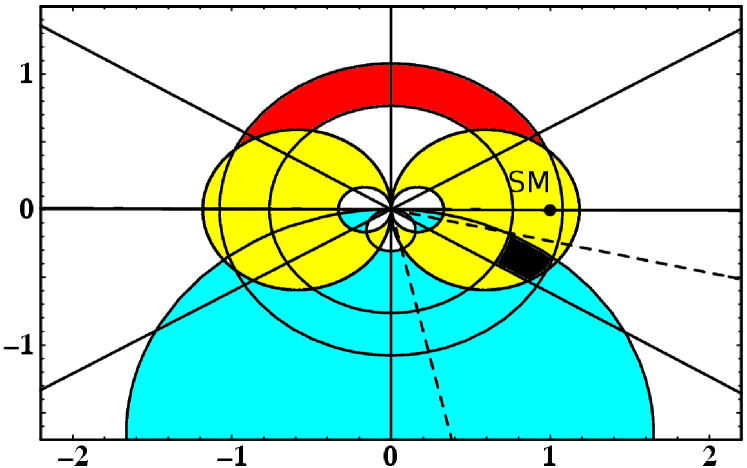
Figure 7: Current experimental bounds in the complex $\Delta_{s}$-plane. The bound from $\Delta M_{s}$ is given by the red (dark-grey) annulus around the origin. The bound from $|\Delta\Gamma_{s}|/\Delta M_{s}$ is given by the yellow (light-grey) region and the bound from $a_{\rm fs}^{s}$ is given by the light-blue (grey) region. The angle $\phi_{s}^{\Delta}$ can be extracted from $|\Delta\Gamma_{s}|$ (solid lines) with a four–fold ambiguity — each of the four regions is bounded by a solid ray and the x-axis — or from the angular analysis in $B_{s}\to J/\Psi\phi$ (dashed line). This constraint also has a four–fold ambiguity if no assumptions on the strong phases $\delta_{1}$ and $\delta_{2}$ are made. The dashed lines limit the region corresponding to the solution in Eq. (90). The Standard Model case corresponds to $\Delta_{s}=1$. The current experimental situation shows a small deviation, which may become significant, if the experimental uncertainties in $\Delta\Gamma_{s}$, $a_{\rm sl}^{s}$ and $\phi_{s}$ will go down in near future.

 

The combined analysis of $\Delta M_{s}$, $\phi_{s}$, $|\Delta\Gamma_{s}|/\Delta M_{s}$ and $a_{\rm sl}^{s}$ in Fig. 7 shows some hints for deviations from the Standard Model. To analyse them further we ignore discrete ambiguities and focus on the solution in the fourth quadrant which is closest to the Standard Model solution $\Delta_{s}=1$. We further do not perform a complete statistical analysis with proper inclusion of all correlations and for simplicity add statistical and systematic errors in quadrature. First we note from Eq. (75) that Eq. (7) implies

$$|\Delta_{s}| = 0.92\pm 0.32{}_{\mbox{\scriptsize(th)}}\pm 0.01{}_{\mbox{\scriptsize(exp)}}$$ (98)

while Eqs. (77) and (90) lead to

$$\frac{\cos\phi_{s}}{|\Delta_{s}|} = 1.93\pm 0.37{}_{\mbox{\scriptsize(th)}}\pm 1.1{}_{\mbox{\scriptsize(exp)}}.$$ (99)

Eqs. (98) and (99) are consistent with $\Delta_{s}=1$, but prefer $|\Delta_{s}|<1$.

Second we observe that both the angular distribution in $\raisebox{7.7pt}{$\scriptscriptstyle(\hskip 8.5pt)$}\!\,\overline{\!B}_{s}\to J/\psi\phi$ giving Eq. (91) and $a_{\rm sl}^{s}$ in Eq. (97) point towards a non-zero $\phi_{s}$. Both analyses involve $\sin\phi_{s}$, the two values inferred are

$$\sin\phi_{s} = -0.71\raisebox{-2.15277pt}{\shortstack[l]{$\scriptstyle+0.48$\\ $\scriptstyle-0.27$}}\qquad\qquad\quad\mbox{from the angular analysis, Eq.~{}(\ref{eqdgexp4}),}$$ (100)

$$\frac{\sin\phi_{s}}{|\Delta_{s}|} = -1.77\pm 0.33{}_{\mbox{\scriptsize(th)}}\pm 1.47{}_{\mbox{\scriptsize(exp)}}\qquad\qquad\mbox{from $a_{\rm sl}$ in Eq.~{}(\ref{eqasldfinal2})}.$$ (101)

In Eq. (101) we have profited from our improved theory prediction in Eq. (78). For $|\Delta_{s}|=1$ the two numbers combine to

$$\sin\phi_{s} = -0.77\pm 0.02{}_{\mbox{\scriptsize(th)}}\pm 0.36{}_{\mbox{\scriptsize(exp)}}.$$ (102)

Relaxing $|\Delta_{s}|$ to its minimal value allowed by Eq. (98), $|\Delta_{s}|=0.59$, changes this result to

$$\sin\phi_{s} = -0.76\pm 0.03{}_{\mbox{\scriptsize(th)}}\pm 0.34{}_{\mbox{\scriptsize(exp)}}.$$ (103)

Either Eq. (102) or Eq. (103) alone imply a deviation from $\phi_{s}=0$ by 2.1$\sigma$, but $\Delta\Gamma_{s}$ in Eq. (91) pulls in the opposite direction, preferring large values of $|\cos\phi_{s}|$ through Eq. (76). Despite of its large error $\Delta\Gamma_{s}$ already gives a powerful lower bound $|\cos\phi_{s}|\geq 0.55$ (so that $|\sin\phi_{s}|\leq 0.84$) at the 1$\sigma$ level because of its large central value in Eq. (91). This can be clearly seen from Fig. 7. However, $\Delta\Gamma_{s}$ is consistent with $\cos\phi_{s}=0$ at the 1.8$\sigma$ level and clearly has no impact on the small $\phi_{s}$ region, which is the relevant region to assess the significance of Eq. (102) in the search for new physics.

In conclusion we find that the data are best fit for $\phi_{s}$ around $-0.88$ corresponding to $\sin\phi_{s}=-0.77$, if $|\Delta_{s}|=1$. The constraint from $|\Delta\Gamma_{s}|$ is less compelling, but slightly prefers $|\Delta_{s}|<0$ and disfavours too large values of $|\sin\phi_{s}|$. The discrepancy between data and the Standard Model is around 2$\sigma$, which is not statistically significant yet. If our results are used to constrain models of new physics one should bear in mind that we have only discussed the solution in the fourth quadrant of the complex $\Delta_{s}$ plane here.

5 A road map for $B_{s}\!-\!\,\overline{\!B}{}_{s}\,$ mixing

Clearly the best way to establish new physics from $B_{s}\!-\!\,\overline{\!B}{}_{s}\,$ mixing is a combination of all observables following the line of Sect. 4.2. In particular it has to be stressed that $A_{\rm CP}^{\rm mix}(B_{s}\to(J/\psi\phi)_{CP\pm})$ and $a_{\rm fs}^{s}$ are not substitutes for each other, but rather give complementary information on the complex $\Delta_{s}$ plane because of their different dependence on $|M_{12}^{s}|$. With the new operator basis presented in this paper it will be possible to determine $\Delta_{s}$ solely from measurements which involve hadronic quantities only in numerically sub-dominant terms. To this end any experimental progress on $|\Delta\Gamma_{s}|$, $a_{\rm fs}^{s}$, the angular distributions of both untagged and tagged $B_{s}\to J/\psi\phi$ decays (with the tagged analysis giving access to $A_{\rm CP}^{\rm mix}(B_{s}\to(J/\psi\phi)_{CP\pm})$) and possibly of other $b\to c\overline{c}s$ decays of the $B_{s}$ meson is highly desirable. Regardless of whether $\sin\phi_{s}$ turns out to be zero or not it is important to measure the sign of $\Delta\Gamma_{s}$. Methods for this are discussed in [44]. Probably the most promising way to determine $\mbox{sign}\,\Delta\Gamma_{s}=\mbox{sign}\,\cos(\phi_{s})$ is the study of $B_{s}\to J/\psi K^{+}K^{-}$ with a scan of the invariant mass of the $(K^{+},K^{-})$ pair around the $\phi$ peak to determine $\mbox{sign}\,\cos\delta_{1,2}$.

Clearly the analysis of the precise measurement of $\Delta M_{s}$ needs a better determination of $f_{B_{s}}^{2}B$. Since any new physics discovery from a quantity involving lattice QCD will be met with scepticism by the scientific community, the lattice collaborations might want to consider to switch to blind analyses in the future. The predictions of both $\Delta\Gamma_{s}/\Delta M_{s}$ and $a_{\rm fs}^{s}$ involve the ratio $\tilde{B}_{S}^{\prime}/B$ in a numerically sub-dominant term. It may be worthwhile to address this ratio directly in lattice computations, because some systematic effects could drop out from the ratio of the two matrix elements.

The quantities discussed in this paper will also profit from higher-order calculations of the short-distance QCD parts. In particular corrections of order $\alpha_{s}/m_{b}$ should be computed to permit a meaningful use of $1/m_{b}$ bag factors computed with lattice QCD or QCD sum rules. A further reduction of the dependence on the renormalisation scale $\mu_{1}$ requires the cumbersome calculation of ${\cal O}(\alpha_{s}^{2})$ corrections. Finally, the reduction of the $1/m_{b}$ corrections with the help of our new operator basis can only be fully appreciated, if the size of the $1/m_{b}^{2}$ terms is indeed small. We have estimated these corrections and indeed found no unnatural enhancement over their natural size.

6 Summary

In this letter we have improved the theoretical accuracy of the mixing quantity $\Gamma_{12}^{q}$, $q=d,s$, by summing the logarithmic terms $\alpha_{s}^{n}z\ln^{n}z$, $z=m_{c}^{2}/m_{b}^{2}$ to all orders $n=1,2,\ldots$ and by introducing a new operator basis, which trades the traditionally used operator $Q_{S}$ of Eq. (8) for $\widetilde{Q}_{S}$ defined in Eq. (16). In the new operator basis the coefficient of the $1/m_{b}$–operator $R_{0}$ is colour–suppressed. We have found that all previously noted pathologies in the sizes of the $1/m_{b}$ and $\alpha_{s}$ corrections were artifacts of the old operator basis. Still, one could achieve the same accuracy with the use of the old basis, if one i) used the coefficients with resummed $\ln z$ terms, ii) added the term of order $N_{c}\alpha_{s}/m_{b}$ which drops from the NLO results of [19, 20, 21] when $\widetilde{Q}_{S}$ is eliminated for $R_{0}$ and iii) fully takes the numerical correlation between $B$ and $B_{S}$ into account. This numerical correlation stems from the smallness of the matrix element $\langle\widetilde{Q}_{S}\rangle$. It is most easily implemented by expressing either $B$ or $B_{S}$ in terms of $\widetilde{B}_{S}$, which is essentially equivalent to our approach.

Our improvements are most relevant for $\mathrm{Re}\,\Gamma_{12}^{q}/M_{12}^{q}$, which enters both $\Delta\Gamma_{q}/\Delta M_{q}$ and new physics scenarios of $a_{\rm fs}^{s}$. In particular, hadronic quantities now appear in these quantities in numerically sub-dominant terms only. We have then discussed how experimental information on $|\Delta\Gamma_{s}|$, $a_{\rm fs}^{s}$, $\phi_{s}$ from the angular distribution of $\raisebox{7.7pt}{$\scriptscriptstyle(\hskip 8.5pt)$}\!\,\overline{\!B}_{s}\to J/\psi\phi$ and $A_{\rm CP}^{\rm mix}(B_{s}\to(J/\psi\phi)_{CP\pm})$ can be efficiently combined to constrain the complex parameter $\Delta_{s}$, which quantifies new physics in $B_{s}\!-\!\,\overline{\!B}{}_{s}\,$ mixing.

Armed with our more precise formulae we have analysed the combined impact of the DØ analyses of the dimuon asymmetry and of the angular distribution in the decay $\raisebox{7.7pt}{$\scriptscriptstyle(\hskip 8.5pt)$}\!\,\overline{\!B}_{s}\to J/\psi\phi$. Here we have assumed that $\phi_{d}$ is free of new physics contributions. This is plausible in view of the constraints on $\phi_{d}$ from global fits to the unitarity triangle [2]. Scanning conservatively over theory uncertainties, we find that $\phi_{s}$ deviates from its Standard Model value by 2 standard deviations.

References

- [1] N. Cabibbo, Phys. Rev. Lett. 10, 531 (1963); M. Kobayashi and T. Maskawa, Prog. Theor. Phys. 49, 652 (1973).
- [2] Updated result of J. Charles et al. [CKMfitter Group], Eur. Phys. J. C 41 (2005) 1 [arXiv:hep-ph/0406184] for the summer conferences 2006, see http://www.slac.stanford.edu/xorg/ckmfitter/ckmresultsbeauty2006.html; updated result of M. Bona et al. [UTfit Collaboration], arXiv:hep-ph/0606167 for the summer conferences 2006, see http://utfit.roma1.infn.it/; updated result of E. Barberio et al. [Heavy Flavor Averaging Group (HFAG)], arXiv:hep-ex/0603003 for the summer conferences 2006, see http://www.slac.stanford.edu/xorg/hfag/.
- [3] The experimental situation is summarised in: M. Hazumi, plenary talk at 33rd International Conference On High Energy Physics (ICHEP 06), 26 Jul – 2 Aug 2006, Moscow, Russia.
- [4] D. Chang, A. Masiero and H. Murayama, Phys. Rev. D 67, 075013 (2003) [arXiv:hep-ph/0205111].
- [5] Effects of the model in [4] on mixing have been studied in: S. Jäger and U. Nierste, Eur. Phys. J. C 33, S256 (2004) [arXiv:hep-ph/0312145]; S. Jäger and U. Nierste, in Proceedings of the 12th International Conference On Supersymmetry And Unification Of Fundamental Interactions (SUSY 04), 17-23 Jun 2004, Tsukuba, Japan, p. 675-678, Ed. K. Hagiwara, J. Kanzaki, N. Okada [hep-ph/0410360]; S. Jäger, hep-ph/0505243, to appear in the Proceedings of the XLth Rencontres de Moriond, Electroweak Interactions and Unified Theories, 5-12 Mar 2005, La Thuile, Aosta Valley, Italy, Ed. J. Tran Thanh Van.
- [6] K. Anikeev et al., physics at the Tevatron: Run II and beyond, [hep-ph/0201071], Chapters 1.3 and 8.3.
- [7] E. H. Thorndike, Ann. Rev. Nucl. Part. Sci. 35 (1985) 195; J. S. Hagelin and M. B. Wise, Nucl. Phys. B 189 (1981) 87; J. S. Hagelin, Nucl. Phys. B 193 (1981) 123; A. J. Buras, W. Slominski and H. Steger, Nucl. Phys. B 245 (1984) 369. R. N. Cahn and M. P. Worah, Phys. Rev. D 60 (1999) 076006;
- [8] U. Nierste, [hep-ph/0406300], in: Proceedings of the XXXIXth Rencontres de Moriond, Electroweak Interactions and Unified Theories, 21-28 Mar 2004, La Thuile, Aosta Valley, Italy, Ed. J. Tran Thanh Van.
- [9] A.J. Buras, M. Jamin and P.H. Weisz, Nucl. Phys. B347, 491 (1990).
- [10] A. Abulencia et al. [CDF Collaboration], arXiv:hep-ex/0609040; A. Abulencia [CDF - Run II Collaboration], Phys. Rev. Lett. 97 (2006) 062003 [arXiv:hep-ex/0606027]; V. M. Abazov et al. [DØ Collaboration], Phys. Rev. Lett. 97 (2006) 021802 [arXiv:hep-ex/0603029].
- [11] M. Ciuchini and L. Silvestrini, Phys. Rev. Lett. 97, 021803 (2006) [arXiv:hep-ph/0603114]; M. Endo and S. Mishima, Phys. Lett. B 640 (2006) 205 [arXiv:hep-ph/0603251]; Z. Ligeti, M. Papucci and G. Perez, Phys. Rev. Lett. 97 (2006) 101801 [arXiv:hep-ph/0604112]; J. Foster, K. i. Okumura and L. Roszkowski, arXiv:hep-ph/0604121; P. Ball and R. Fleischer, arXiv:hep-ph/0604249; G. Isidori and P. Paradisi, Phys. Lett. B 639, 499 (2006) [arXiv:hep-ph/0605012]; S. Khalil, Phys. Rev. D 74 (2006) 035005 [arXiv:hep-ph/0605021]; A. Datta, Phys. Rev. D 74 (2006) 014022 [arXiv:hep-ph/0605039]; S. Baek, JHEP 0609 (2006) 077 [arXiv:hep-ph/0605182]; X. G. He and G. Valencia, Phys. Rev. D 74 (2006) 013011 [arXiv:hep-ph/0605202]; R. Arnowitt, B. Dutta, B. Hu and S. Oh, Phys. Lett. B 641 (2006) 305 [arXiv:hep-ph/0606130]; S. Baek, J. H. Jeon and C. S. Kim, Phys. Lett. B 641 (2006) 183 [arXiv:hep-ph/0607113]; B. Dutta and Y. Mimura, arXiv:hep-ph/0607147; S. Chang, C. S. Kim and J. Song, arXiv:hep-ph/0607313; F. J. Botella, G. C. Branco and M. Nebot, arXiv:hep-ph/0608100; S. Nandi and J. P. Saha, arXiv:hep-ph/0608341; G. Xiangdong, C. S. Li and L. L. Yang, arXiv:hep-ph/0609269; R. M. Wang, G. R. Lu, E. K. Wang and Y. D. Yang, arXiv:hep-ph/0609276; L. x. Lu and Z. j. Xiao, arXiv:hep-ph/0609279; M. Blanke and A. J. Buras, arXiv:hep-ph/0610037.
- [12] M. Blanke, A. J. Buras, D. Guadagnoli and C. Tarantino, arXiv:hep-ph/0604057; M. Blanke, A. J. Buras, A. Poschenrieder, C. Tarantino, S. Uhlig and A. Weiler, arXiv:hep-ph/0605214;
- [13] Z. Ligeti, M. Papucci and G. Perez, Phys. Rev. Lett. 97 (2006) 101801 [arXiv:hep-ph/0604112];
- [14] Y. Grossman, Y. Nir and G. Raz, Phys. Rev. Lett. 97 (2006) 151801 [arXiv:hep-ph/0605028].
- [15] Talks by D. Glenzinski (plenary), T. Moulik and S. Giagu at 33rd International Conference On High Energy Physics (ICHEP 06), 26 Jul – 2 Aug 2006, Moscow, Russia.
- [16] A.J. Buras, M. Jamin, M.E. Lautenbacher and P.H. Weisz, Nucl. Phys. B370, 69 (1992); Addendum-ibid. B375, 501 (1992). M. Ciuchini, E. Franco, G. Martinelli, L. Reina, Nucl. Phys. B415, 403 (1994).
- [17] E. Franco, M. Lusignoli and A. Pugliese, Nucl. Phys. B194, 403 (1982); L.L. Chau, Phys. Rep. 95, 1 (1983); M.B. Voloshin, N.G. Uraltsev, V.A. Khoze and M.A. Shifman, Sov. J. Nucl. Phys. 46, 112 (1987); A. Datta, E.A. Paschos and U. Türke, Phys. Lett. B196, 382 (1987); A. Datta, E.A. Paschos and Y.L. Wu, Nucl. Phys. B311, 35 (1988).
- [18] M. Beneke, G. Buchalla and I. Dunietz, Phys. Rev. D54, 4419 (1996).
- [19] M. Beneke, G. Buchalla, C. Greub, A. Lenz and U. Nierste, Phys. Lett. B 459 (1999) 631 [arXiv:hep-ph/9808385].
- [20] M. Ciuchini, E. Franco, V. Lubicz, F. Mescia and C. Tarantino, JHEP 0308 (2003) 031 [arXiv:hep-ph/0308029].
- [21] M. Beneke, G. Buchalla, A. Lenz and U. Nierste, Phys. Lett. B 576 (2003) 173 [arXiv:hep-ph/0307344].
- [22] D. Becirevic, V. Gimenez, G. Martinelli, M. Papinutto and J. Reyes, JHEP 0204 (2002) 025 [arXiv:hep-lat/0110091].
- [23] A. S. Dighe, T. Hurth, C. S. Kim and T. Yoshikawa, Nucl. Phys. B 624 (2002) 377 [arXiv:hep-ph/0109088].
-
[24]
E. Dalgic et al.,
arXiv:hep-lat/0610104;
J. Shigemitsu for HPQCD Collaboration, talk at LATTICE 2006,
http://www.physics.utah.edu/lat06/abstracts/sessions/weak/s1//ShigemitsuJunko.pdf. - [25] M. Beneke, G. Buchalla, C. Greub, A. Lenz and U. Nierste, Nucl. Phys. B 639 (2002) 389 [arXiv:hep-ph/0202106].
- [26] B. Aubert et al. [BABAR Collaboration], Phys. Rev. Lett. 93 (2004) 011803 [arXiv:hep-ex/0404017]. G. Corcella and A. H. Hoang, Nucl. Phys. Proc. Suppl. 133 (2004) 186 [arXiv:hep-ph/0311004]. M. Eidemuller, Phys. Rev. D 67 (2003) 113002 [arXiv:hep-ph/0207237]. J. H. Kuhn and M. Steinhauser, Nucl. Phys. B 619 (2001) 588 [Erratum-ibid. B 640 (2002) 415] [arXiv:hep-ph/0109084]. P. A. Baikov, K. G. Chetyrkin and J. H. Kuhn, Phys. Rev. Lett. 95 (2005) 012003 [arXiv:hep-ph/0412350]. E. Gamiz, M. Jamin, A. Pich, J. Prades and F. Schwab, arXiv:hep-ph/0505122. S. Narison, Phys. Lett. B 626, 101 (2005) [arXiv:hep-ph/0501208]. E. Brubaker et al. [Tevatron Electroweak Working Group], arXiv:hep-ex/0608032.
- [27] W. M. Yao et al. [Particle Data Group], J. Phys. G 33 (2006) 1.
- [28] S. Bethke, arXiv:hep-ex/0606035.
- [29] M. Jamin and B. O. Lange, Phys. Rev. D 65 (2002) 056005 [arXiv:hep-ph/0108135].
- [30] J. G. Korner, A. I. Onishchenko, A. A. Petrov and A. A. Pivovarov, Phys. Rev. Lett. 91 (2003) 192002 [arXiv:hep-ph/0306032].
- [31] C. S. Huang, A. Zhang and S. L. Zhu, Eur. Phys. J. C 21 (2001) 313 [arXiv:hep-ph/0011145].
- [32] S. Hashimoto and T. Onogi, arXiv:hep-ph/0407221; S. Hashimoto, Int. J. Mod. Phys. A 20 (2005) 5133 [arXiv:hep-ph/0411126]; M. Okamoto, PoS LAT2005 (2006) 013 [arXiv:hep-lat/0510113].
- [33] A. Ali Khan et al. [CP-PACS Collaboration], Phys. Rev. D 64 (2001) 054504 [arXiv:hep-lat/0103020]; A. Ali Khan et al. [CP-PACS Collaboration], Phys. Rev. D 64 (2001) 034505 [arXiv:hep-lat/0010009]; C. Bernard et al. [MILC Collaboration], Phys. Rev. D 66 (2002) 094501 [arXiv:hep-lat/0206016]; S. Collins, C. T. H. Davies, U. M. Heller, A. Ali Khan, J. Shigemitsu, J. H. Sloan and C. Morningstar, Phys. Rev. D 60 (1999) 074504 [arXiv:hep-lat/9901001].
- [34] S. Aoki et al. [JLQCD Collaboration], Phys. Rev. Lett. 91 (2003) 212001 [arXiv:hep-ph/0307039].
- [35] V. Gimenez and J. Reyes, Nucl. Phys. Proc. Suppl. 94 (2001) 350 [arXiv:hep-lat/0010048].
- [36] N. Yamada et al. [JLQCD Collaboration], Nucl. Phys. Proc. Suppl. 106 (2002) 397 [arXiv:hep-lat/0110087].
- [37] M. Wingate, C. T. H. Davies, A. Gray, G. P. Lepage and J. Shigemitsu, Phys. Rev. Lett. 92 (2004) 162001 [arXiv:hep-ph/0311130]; A. Gray et al. [HPQCD Collaboration], Phys. Rev. Lett. 95 (2005) 212001 [arXiv:hep-lat/0507015].
- [38] M. Beneke and A. Lenz, J. Phys. G 27 (2001) 1219 [arXiv:hep-ph/0012222].
- [39] U. Nierste, in Proc. of the 5th International Symposium on Radiative Corrections (RADCOR 2000) ed. Howard E. Haber, arXiv:hep-ph/0105215;
- [40] A. Lenz, arXiv:hep-ph/0412007;
- [41] M. Bona et al. [UTfit Collaboration], arXiv:hep-ph/0605213.
- [42] Y. Grossman, Y. Nir and M. P. Worah, Phys. Lett. B 407 (1997) 307 [arXiv:hep-ph/9704287].
- [43] Y. Grossman, Phys. Lett. B 380 (1996) 99 [arXiv:hep-ph/9603244].
- [44] I. Dunietz, R. Fleischer and U. Nierste, Phys. Rev. D 63 (2001) 114015 [arXiv:hep-ph/0012219].
- [45] K. Hartkorn and H. G. Moser, Eur. Phys. J. C 8 (1999) 381.
- [46] A. S. Dighe, I. Dunietz, H. J. Lipkin and J. L. Rosner, Phys. Lett. B 369 (1996) 144 [arXiv:hep-ph/9511363]. A. S. Dighe, I. Dunietz and R. Fleischer, Eur. Phys. J. C 6 (1999) 647 [arXiv:hep-ph/9804253].
- [47] M. A. Shifman and M. B. Voloshin, Sov. J. Nucl. Phys. 47 (1988) 511 [Yad. Fiz. 47 (1988) 801].
- [48] R. Aleksan, A. Le Yaouanc, L. Oliver, O. Pene and J. C. Raynal, Phys. Lett. B 316 (1993) 567.
- [49] D. Acosta et al. [CDF Collaboration], Phys. Rev. Lett. 94 (2005) 101803 [arXiv:hep-ex/0412057]; DØ collaboration, conference note 5052, http://www-do.fnal.gov/.
- [50] V. M. Abazov et al. [D0 Collaboration], Phys. Rev. Lett. 98 (2007) 121801 [arXiv:hep-ex/0701012].
- [51] V. M. Abazov et al. [D0 Collaboration], arXiv:hep-ex/0701007.
- [52] V. M. Abazov et al. [D0 Collaboration], Phys. Rev. D 74 (2006) 092001 [arXiv:hep-ex/0609014].
- [53] G. Borissov, D. Zieminska and A. Chandra, DØ conference note no. 5189, http://www-do.fnal.gov. For an update see: V. Abazov et al. [D0 Collaboration], arXiv:hep-ex/0702030.