FERMILAB-PUB-06-457-T

CERN-PH-TH/2006-255

UAB-FT-617

hep-ph/0612166

Huge right-handed current effects in $B\to K^{*}(K\pi)\ell^{+}\ell^{-}$ in
supersymmetry

Enrico Lunghi¹, Joaquim Matias²

¹ Fermi National Accelerator Laboratory
P.O. Box 500, Batavia, IL 60510-0500, USA
E-mail: lunghi@fnal.gov
² IFAE, Universitat Autònoma de Barcelona
08193 Bellaterra, Barcelona, Spain
E-mail: matias@ecm.ub.es

Abstract

Transverse asymmetries in the decay $B\to K^{*}(K\pi)\ell^{+}\ell^{-}$ are an extremely sensitive probe of right-handed flavour-changing neutral currents. We show how to include the contribution from the chiral partner of the electromagnetic operator on the transverse asymmetries at NLO in QCD factorization. We then consider supersymmetric models with non-minimal flavour violation in the down-squark sector. We include all the relevant experimental constraints and present a numerical formula for $B\to X_{s}\gamma$ that takes into account the most recent NNLO calculations. We show that the flavour-changing parameters of these models are poorly constrained by present data and allow for large effects on the transverse asymmetries that we consider.

1 Introduction

B decays offer a unique opportunity to explore the flavour structure of the theory lying beyond the Standard Model [3, 4, 5, 6, 7]. Given the scenario depicted by present data, the search for new physics in the flavour sector is evolving more and more toward precision analyses. On the one side, new methods are being developed to produce more accurate predictions focusing, in particular, on the problem of large $\Lambda/m_{b}$ corrections (see for instance Ref. [8] in the context of $B\to\pi\pi$ decays and Ref. [9] for $B_{s}\to KK$ decays). On the other side, new observables are being proposed to test specific types of new physics (presence of right-handed currents [10, 11, 12, 13], isospin breaking beyond the SM [14, 15], etc.). In particular, one of the most important targets of present searches is to find observables that can test the chiral structure of the fundamental theory lying beyond the SM.

In a previous paper [13] a set of observables based on the angular distribution of the decay $B\to K^{*}(K\pi)\ell^{+}\ell^{-}$ were analysed at NLO in the SM in the framework of QCD Factorization. They provide information of the $K^{*}$ spin amplitudes [16, 11, 12] that are useful to search for right-handed currents. The goal was to identify the most robust observables, i.e., those less affected by hadronic uncertainties, to search for new physics originated by right-handed currents. The most promising observables were found to be the transverse asymmetries (see Ref. [13]) due to the exact cancellation, at leading order, of the poorly known soft form factors. This cancellation is basically not spoiled when including NLO corrections.

In Ref. [13] a model-independent analysis was done to test the possible impact of right-handed currents on those promising observables. It remained to be explored whether a well-motivated model, once all kinds of constraints are included, can still naturally lead to large deviations.

There are several models that can produce right-handed currents, such as, left-right-symmetric models with or without spontaneous CP violation. However, some of these models have already been ruled out (see for instance Ref. [17]). The aim of the present paper is to show the possible impact that a well-motivated Minimal Supersymmetric Model (MSSM), with non-minimal flavour changing and R-parity conservation, has on the transverse asymmetries and the polarization fraction (see [18] for universal extra-dimensions case). The corresponding integrated observables are analysed as well. Because of its experimental interest [19], we have included also the prediction for the longitudinal fraction of $K^{*}$ polarization, even though it was already shown in [13] that it is a difficult task to extract clean information concerning new physics out of this observable. Apart from uncertainties coming from soft form factors, another important source of theoretical error comes from the uncontrolled $\Lambda/m_{b}$ contributions. In order to explore the impact of these unknown corrections, we allow for a $\pm 10\%$ error (this comes from taking $\Lambda$ in a range between 200 and 400 MeV, $m_{b}$ of the order of 5 GeV, and assuming all coefficients of order 1) on each individual amplitude.

The structure of the paper is the following. In Section 2, we generalize the transverse amplitudes at NLO in order to incorporate the extra contribution coming from the chiral partner of the electromagnetic operator and we define the observables. In Section 3 we describe the structure of the squark mass matrix to show how the sources of flavour changing enter. We will focus on the dominant contribution coming from penguin diagrams involving a gluino and down squarks, and we will use the complete result for the Wilson coefficients following [20] that generalizes the results given in the approximate formulae [21, 22]. We will chose a minimal set of free parameters (gluino and down squark masses together with only one mass insertion), which are sufficient to illustrate the large impact on the interesting observables. Finally we impose in Section 4 all relevant experimental constraints, including the very last results for $B\to X_{s}\gamma$ [23, 24, 25, 26]. Next, we describe in Section 5 the numerical results focusing on some representative cases to show the huge impact that the model has on these observables. We also show the constraint on the squark and gluino masses implied by a measurement of a large effect on the transverse asymmetries. We conclude in Section 6.

2 The transverse asymmetries

The effective Hamiltonian describing the quark transition $b\to sl^{+}l^{-}$ [10, 16, 11, 12] is given by [27, 28, 29, 30]:

$${\mathcal{H}}_{\rm eff}=-\frac{4G_{F}}{\sqrt{2}}V_{tb}V_{ts}^{*}\sum_{i=1}^{10}[C_{i}(\mu){\mathcal{O}}_{i}(\mu)+C_{i}^{\prime}(\mu){\mathcal{O}}_{i}^{\prime}(\mu)],$$ (1)

where in addition to the SM operators we have added the chirally flipped partners. For the complete set of operators (${\mathcal{O}}_{i}^{(\prime)}(\mu)$) and Wilson coefficients ($C_{i}^{(\prime)}(\mu)$) in the SM and beyond, we refer the reader to [27, 28, 29, 30, 17, 31, 32, 33, 34, 35]. In what follows we will use the same conventions as in [13].

We will be specially interested here in the two electromagnetic partner operators:

$${\mathcal{O}}_{7}=\frac{e}{16\pi^{2}}m_{b}(\bar{s}\sigma_{\mu\nu}P_{R}b)F^{\mu\nu},\quad{\mathcal{O}}_{7}^{\prime}=\frac{e}{16\pi^{2}}m_{b}(\bar{s}\sigma_{\mu\nu}P_{L}b)F^{\mu\nu}$$ (2)

and in the semileptonic operators:

$${\mathcal{O}}_{9}=\frac{e^{2}}{16\pi^{2}}(\bar{s}\gamma_{\mu}P_{L}b)(\bar{l}\gamma^{\mu}l),\quad{\mathcal{O}}_{10}=\frac{e^{2}}{16\pi^{2}}(\bar{s}\gamma_{\mu}P_{L}b)(\bar{l}\gamma^{\mu}\gamma_{5}l),$$ (3)

where $P_{L,R}=(1\mp\gamma_{5})/2$ and $m_{b}\equiv m_{b}(\mu)$ is the running mass in the $\overline{\mbox{MS}}$ scheme. From the effective Hamiltonian it is straightforward to compute the matrix element for the decay $B\rightarrow K^{*}(\rightarrow K\pi)l^{+}l^{-}$:

$${\mathcal{M}} = \frac{G_{F}\alpha}{\sqrt{2}\pi}V_{tb}V_{ts}^{*}\;\bigg{\{}$$ (4)

$$\bigg{[}C_{9}^{\rm{eff}}\langle K\pi|(\bar{s}\gamma^{\mu}P_{L}b)|B\rangle-\frac{2m_{b}}{q^{2}}\langle K\pi|\bar{s}i\sigma^{\mu\nu}q_{\nu}(C_{7}^{\rm{eff}}P_{R}+{C_{7}^{\rm{eff}}}^{\prime}P_{L})b|B\rangle\bigg{]}(\bar{l}\gamma_{\mu}l)$$

$$+\;C_{10}\langle K\pi|(\bar{s}\gamma^{\mu}P_{L}b)|B\rangle(\bar{l}\gamma_{\mu}\gamma_{5}l)\bigg{\}},$$

where $q$ is the four-momentum of the lepton pair. The explicit form of the four hadronic matrix elements can be found in [13].

Our goal in this section will be to generalize the formulae in [13] to describe the angular distribution and transversity amplitudes at NLO, in the presence of the chirally flipped operator ${\cal O}^{\prime}_{7}$. The transversity amplitudes corresponding to the four physical $K^{*}$ spin amplitudes $A_{\bot}$, $A_{\|}$, $A_{0}$ and $A_{t}$ are related to the helicity amplitudes, also used in literature through:

$$A_{\bot,\|}=(H_{+1}\mp H_{-1})/\sqrt{2},\quad A_{0}=H_{0},\quad A_{t}=H_{t}.$$ (5)

Each spin amplitude splits in a left-handed and a right-handed component and in our observables discussed below we introduce the shorthand notation:

$$A_{i}A^{*}_{j}\equiv A_{iL}(s)A^{*}_{jL}(s)+A_{iR}(s)A^{*}_{jR}(s)\quad(i,j=0,\|,\perp).$$ (6)

The generalization to include the impact of the dipole operator $O_{7}^{\prime}$ is achieved by taking the transversity amplitudes (we focus here on $A_{\bot L,R}$, $A_{\|L,R}$ and $A_{0L,R}$) obtained from the above matrix element:

$$A_{\bot L,R}=N\sqrt{2}\lambda^{1/2}\bigg{[}(C_{9}^{\rm{eff}}\mp C_{10})\frac{V(s)}{m_{B}+m_{K^{*}}}+\frac{2m_{b}}{s}(C_{7}^{\rm{eff}}+{C_{7}^{\rm{eff}}}^{\prime})T_{1}(s)\bigg{]},$$ (7)

$$A_{\|L,R}=-N\sqrt{2}(m_{B}^{2}-m_{K^{*}}^{2})\bigg{[}(C_{9}^{\rm{eff}}\mp C_{10})\frac{A_{1}(s)}{m_{B}-m_{K^{*}}}+\frac{2m_{b}}{s}(C_{7}^{\rm{eff}}-{C_{7}^{\rm{eff}}}^{\prime})T_{2}(s)\bigg{]},$$ (8)

$$A_{0L,R} = -\frac{N}{2m_{K^{*}}\sqrt{s}}\bigg{[}(C_{9}^{\rm{eff}}\mp C_{10})\bigg{\{}(m_{B}^{2}-m_{K^{*}}^{2}-s)(m_{B}+m_{K^{*}})A_{1}(s)-\lambda\frac{A_{2}(s)}{m_{B}+m_{K^{*}}}\bigg{\}}$$ (9)

$$+ {2m_{b}}(C_{7}^{\rm{eff}}-{C_{7}^{\rm{eff}}}^{\prime})\bigg{\{}(m_{B}^{2}+3m_{K^{*}}^{2}-s)T_{2}(s)-\frac{\lambda}{m_{B}^{2}-m_{K^{*}}^{2}}T_{3}(s)\bigg{\}}\bigg{]},$$

where $\lambda$ and $N$ are defined as in [13], and perform the following substitutions:

$$(C_{7}^{\rm{eff}}+{C_{7}^{\rm{eff}}}^{\prime})T_{i}\rightarrow{\cal T}_{i}^{+},\quad(C_{7}^{\rm{eff}}-{C_{7}^{\rm{eff}}}^{\prime})T_{i}\rightarrow{\cal T}_{i}^{-},\quad C_{9}^{\rm{eff}}\rightarrow C_{9}\quad(i=1,2,3),$$ (10)

with the Wilson coefficients $C_{9,10}$ taken at NNLL order (in the sense of Ref. [37]). The ${\cal T}_{i}^{\pm}$ in Eq. (10) are given by

$${\cal T}_{1}^{\pm}={\cal T}^{\pm}_{\perp},\quad{\cal T}_{2}^{-}=\frac{2E_{{K^{*}}}}{m_{B}}{\cal T}_{\perp}^{-},\quad{\cal T}_{3}^{-}={\cal T}_{\perp}^{-}+{\cal T}_{\parallel}^{-}.$$ (11)

${\cal T}_{a}^{\pm}$ ($a=\bot,\|$) contain factorizable (f) and non-factorizable (nf) contributions [37] and it is defined by:

$${\cal T}_{\perp}^{\pm} = \xi_{\perp}(0)\Bigg{\{}C_{\perp}^{(0,\pm)}\frac{1}{(1-s/m_{B}^{2})^{2}}+\frac{\alpha_{s}}{3\pi}\Bigg{[}\frac{C_{\perp}^{(1,\pm)}}{(1-s/m_{B}^{2})^{2}}+\kappa_{\perp}\lambda^{-1}_{B,+}\int_{0}^{1}du\,\Phi_{K^{*},\perp}(u)$$ (12)

$$\times [T_{\perp,+}^{(\mathrm{f}\pm)}(u)+T_{\perp,+}^{(\mathrm{nf}\pm)}(u)]\Bigg{]}\Bigg{\}},$$

where the symbol $\pm$ stands for the substitution of $C_{7}^{\rm{eff}}\to C_{7}^{\rm{eff}}+{C_{7}^{\rm{eff}}}^{\prime}$ (for $+$) and $C_{7}^{\rm{eff}}\to C_{7}^{\rm{eff}}-{C_{7}^{\rm{eff}}}^{\prime}$ (for $-$), wherever $C_{7}^{\rm{eff}}$ appears. ${\cal T}_{\|}^{-}$ is defined in a completely analogous way from the definition of ${\cal T}_{\|}$ [37]; however, in this case, the substitution is always $C_{7}^{\rm{eff}}\to C_{7}^{\rm{eff}}-{C_{7}^{\rm{eff}}}^{\prime}$. The Wilson coefficients of the standard basis ${\cal O}_{i}$ run at NLO, following [38], while the running of the chirally flipped ${C_{7}^{\rm{eff}}}^{\prime}$ is done at LO following [39].

We can now insert the complete transverse amplitudes into our set of observables:

$$A^{(1)}_{{T}}({s})=\frac{-2{\rm{Re}}(A_{\|}{A}_{\bot}^{*})}{|{A}_{\bot}|^{2}+|A_{\|}|^{2}},\quad A^{(2)}_{{T}}({s})=\frac{|{A}_{\bot}|^{2}-|A_{\|}|^{2}}{|{A}_{\bot}|^{2}+|A_{\|}|^{2}},\quad F_{L}(s)=\frac{|{A}_{0}|^{2}}{|{A}_{0}|^{2}+|{A}_{\|}|^{2}+|A_{\perp}|^{2}},$$ (13)

corresponding to the transverse asymmetries and the $K^{*}$ polarization fraction. The reason to choose this small subset of observables is due to the robustness of $A^{(1,2)}_{{T}}({s})$ in front of the NLO corrections, as it was found in [13], and to the experimental interest of $F_{L}(s)$. However, we will show here that it is difficult to extract clean information concerning new physics from this observable $F_{L}(s)$. We will also consider the corresponding integrated quantities: ${\mathcal{A}}^{(1)}_{{T}}$, ${\mathcal{A}}^{(2)}_{{T}}$ obtained integrating numerator and denominator of the corresponding observables over the low-$s$ region $1\;{\rm GeV^{2}}<s<6\;{\rm GeV^{2}}$. It is interesting to observe that working in the helicity basis defined in Eq. (5) within the SM (where in particular ${C_{7}^{\rm{eff}}}^{\prime}=0$) one recovers the quark-model prediction $H_{+1}=0$. The physical reason is that the combination of the $s$ quark produced with an helicity -1/2 by weak interactions, once combined with the light quark can only form a $K^{*}$ in an helicity state -1 or 0. This translates approximately in $A_{T}^{(1)}\sim 1$ and $A_{T}^{(2)}\sim 0$ in the SM. Indeed the different sign contribution of ${C_{7}^{\rm{eff}}}^{\prime}$ in $A_{\bot}$, as it can be seen in Eq.(7), versus $A_{\|}$ (Eq. (8)) generates an interference term proportional to $4{{C_{7}^{\rm{eff}}}^{\prime}}^{2}{\hat{m}_{b}}^{2}/{\hat{s}}^{2}$ strongly sensitive to the presence of right-handed currents.

In a previous paper [13] we observed in a model-independent way that a relatively small contribution to ${C_{7}^{\rm{eff}}}^{\prime}$ has a strong impact on those asymmetries. On the other hand, in Ref. [13] it was also shown that the impact of $C_{9,10}$ is quite small and subleading when compared with ${C_{7}^{\rm{eff}}}^{\prime}$ (due to the 2 ${\hat{m}_{b}}/{\hat{s}}$ factor), once the constraint from $B\to X_{s}\ell^{+}\ell^{-}$ is taken into account (see Fig.5 and 6 in [13]). The inclusion of their chiral partners via the substitutions: $C^{(\mathrm{eff})}_{9,10}\to C^{(\mathrm{eff})}_{9,10}+C^{(\mathrm{eff})\prime}_{9,10}$ in Eq. (7), $C_{9,10}^{(\mathrm{eff})}\to C^{(\mathrm{eff})}_{9,10}-C^{(\mathrm{eff})\prime}_{9,10}$ in Eqs. (8) and (9) entering at the same level as ${\cal O}_{9,10}$ will have a similarly small impact.

For this reason the present analysis will focus on models with large effects on ${C_{7}^{\rm{eff}}}^{\prime}$ only. In the next section we will check it explicitly for a well-motivated supersymmetric model, taking into account all possible constraints.

Another observable that is very sensitive to a non-vanishing ${C_{7}^{\rm{eff}}}^{\prime}$ is the time-dependent CP asymmetry in $B\to K^{*}\gamma$ [40, 42, 41] whose theoretical errors on the leading power contributions are small. It is very important to test both the $q^{2}=0$ limit with this asymmetry and the whole spectrum using the asymmetries $A_{T}^{(1)}(s)$ and $A_{T}^{(2)}(s)$. However, at the experimental level at LHCb the time-dependent analysis in $B\to K^{*}\gamma$ requires to look at a final state, which is a CP eigenstate ($K^{*0}\to K^{0}_{S}\pi^{0}$). This is considered very difficult at LHCb [43] but possible at the B-Factories [44]. Despite of this, a measurement of both set of observables $B\to K^{*}\gamma$ and $A_{T}^{(1)}(s)$ and $A_{T}^{(2)}(s)$ with high precision could be also useful to set bounds on the sub-leading $O_{9,10}^{(^{\prime})}$ contributions.

3 Gluino-mediated FCNC

As an example of a new physics model that allows for large contributions to ${C_{7}^{\rm{eff}}}^{\prime}$, we consider an R-parity-conserving MSSM with non-minimal flavour changing in the down-squarks soft-breaking terms. We define the model at the electroweak scale and implement the resummation of large-$\tan\beta$ effects [45, 46, 47, 48, 49, 50] in the quark mass eigenstate basis [51]. We adopt the notation and conventions of Ref. [51].

The soft-breaking terms are given in the physical super-CKM basis. In this basis, rigid superfield rotations are used to diagonalize the physical quark mass matrices, i.e., this is the basis in which, after the integration of the soft-breaking terms, the quark masses and the CKM matrix coincide with the observed ones. The down-squark mass matrix in the physical SCKM basis is

$${\cal M}^{2}_{\tilde{d}} = \pmatrix{m^{2}_{d,LL}+F_{d,LL}+D_{d,LL}&m^{2}_{d,LR}+F_{d,LR}\cr\left(m^{2}_{d,LR}+F_{d,LR}\right)^{\dagger}&m^{2}_{d,RR}+F_{d,RR}+D_{d,RR}\cr}$$ (14)

where the $F$-terms are $F_{d,LL}=F_{d,RR}^{\dagger}=m_{d}^{(0)\dagger}m_{d}^{(0)}$, $F_{d,LR}=-\mu\tan\beta m_{d}^{(0)\dagger}$ and the $D$-terms are $D_{d,LL}=m_{Z}^{2}\cos 2\beta(-1/2+\sin^{2}\theta_{W}/3)$, $D_{d,RR}=-m_{Z}^{2}\cos 2\beta\sin^{2}\theta_{W}/3$. In the above formulae, $m_{d}^{(0)}$ is the tree-level down-quark mass matrix: the physical mass matrix is obtained only after adding the supersymmetric corrections, $m_{d}=m_{d}^{(0)}+\delta m_{d}={\rm diag}(m_{d},m_{s},m_{b})$.

We parametrize off-diagonal entries of the down-squark mass matrix in terms of mass insertions ($A,B=L,R$):

$$\left(\delta^{d}_{AB}\right)_{ij}\equiv\left(m_{d,AB}^{2}\right)_{ij}/\sqrt{\left(m^{2}_{d,AA}\right)_{ij}\left(m^{2}_{d,BB}\right)_{ij}}\;.$$ (15)

Note that in the numerics we diagonalize exactly the squark mass matrices. After implementing the resummation of the large $\tan\beta$ effects, we use FeynHiggs 2.4.1 [52] to calculate the Higgs spectrum and the $\rho$ parameter.

In a minimal flavour-violating scenario, all contributions to ${C_{7}^{\rm{eff}}}^{\prime}$ are suppressed by a factor $m_{s}/m_{b}$; hence, large effects are possible only if some of the mass insertions are non-vanishing. Let us consider the effect of non-zero mass insertions in the down sector. The main contribution comes from penguin diagrams involving a gluino and down squark. From the approximate expressions given in Ref. [21] we see that only $(\delta^{d}_{RR})_{32}$ and $(\delta^{d}_{LR})_{32}$ contribute; since the latter is strongly enhanced by a factor $m_{\tilde{g}}/m_{b}$, even modest values of this mass insertion (in the $10^{-3}$ range) are sufficient to induce large effects on ${C_{7}^{\rm{eff}}}^{\prime}$. Moreover, since the $m_{\tilde{g}}/m_{b}$ enhancement factor is present exclusively in the contribution to ${C_{7}^{\rm{eff}}}^{\prime}$, a $(\delta^{d}_{LR})_{32}\sim O(10^{-3})$ will have a large impact on ${C_{7}^{\rm{eff}}}^{\prime}$ while being completely irrelevant for any other process.

In the numerical analysis we use the complete formulae for the Wilson coefficients which can be found in Ref. [20]. The most important parameters that we have in this scenario are the gluino mass $m_{\tilde{g}}$, the down squark mass eigenvalues and the normalized insertion $(\delta^{d}_{LR})_{32}$ .

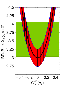
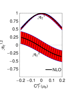
Figure 1: Dependence of the $B\to X_{s}\gamma$ branching ratio and of the integrated transverse asymmetries ${\cal A}_{T}^{1,2}$ on the new physics contribution to the Wilson coefficients ${C_{7}^{\rm{eff}}}^{\prime}(\mu_{b})$. The asymmetries are integrated in the low-$s$ region, $1\;{\rm GeV^{2}}<s<6\;{\rm GeV^{2}}$. The horizontal band on the left plot is the 95% C.L. experimental measurement of ${\cal B}(B\to X_{s}\gamma)$. The dashed region on the right plot correspond to adding all errors in quadrature, including the estimated $\Lambda/m_{b}$ corrections.

4 Experimental constraints

The main constraint on our model comes from the $\bar{B}\to X_{s}\gamma$ decay. The experimental world average for its branching ratio, with a cut $E_{\gamma}>1.6\;{\rm GeV}$ in the $\bar{B}$ rest frame, reads [53]:

$${\cal B}(B\to X_{s}\gamma)^{\rm exp}_{E_{\gamma}>1.6\;{\rm GeV}}=\left(3.55\pm 0.24^{+0.09}_{-0.10}\pm 0.03\right)\times 10^{-4}\;,$$ (16)

yielding at the 95% C.L. range $[3.03,4.07]\times 10^{-4}$. The most recent NNLO results [23, 24] can be reproduced by choosing appropriate renormalization scales in the NLO expressions (see, for instance, Ref. [54, 55]). Using the same numerical inputs as in Ref. [24], and taking $(\mu_{c},\mu_{b},\mu_{0})\simeq(1.3,1.4,160)\;{\rm GeV}$, the NLO central value of the branching ratio coincides with the NNLO one. Other choices of the scales $\mu_{b,c}$ yield the same numerical central value but require to push either one of the two scales dangerously close to the non-perturbative regime. In order to implement the estimate of the new class of power corrections identified in Ref. [25] and of the analysis of the photon energy spectrum presented in Ref. [26], we first calculated the NLO branching ratio with $E_{\gamma}>1\;{\rm GeV}$, adopting the above choice of input values and scales, then subtracted 1.65%, as suggested by the analysis of Ref. [25], and finally multiplied by the conversion factor [26]

$$T={\cal B}_{E_{\gamma}>1.6\;{\rm GeV}}/{\cal B}_{E_{\gamma}>1\;{\rm GeV}}=0.93^{+0.03}_{-0.05}({\rm pert})\pm 0.02({\rm hadr})\pm 0.02({\rm pars})\;.$$ (17)

We obtain the following numerical formula in which we allow for arbitrary new physics contributions to the matching conditions (at the scale $\mu_{0}=160\;{\rm GeV}$) of the leading ($C_{7,8}^{(0)}$ and $C_{7,8}^{\prime(0)}$) and next-to-leading ($C_{7,8}^{(1)}$) Wilson coefficients:

$a=2.98$	$a_{7}=-7.184+0.612\;i$	$b_{77}=0.084$	$b_{7}=-0.075$
$a_{77}=4.743$	$a_{8}=-2.225-0.557\;i$	$b_{88}=0.007$	$b_{8}=-0.022$
$a_{88}=0.789$	$a_{78}=2.454-0.884\;i$	$b_{78}=0.025$

Table 1: Numerical values of the coefficients that enter Eq. (18).

$$\hskip-22.76228pt{\cal B}(\bar{B}\to X_{s}\gamma)_{E_{\gamma}>1.6\;{\rm GeV}}^{\rm th} = 10^{-4}\Bigg{[}a+a_{77}\,\left(|\delta C_{7}^{(0)}|^{2}+|\delta C_{7}^{\prime(0)}|^{2}\right)+a_{88}\,\left(|\delta C_{8}^{(0)}|^{2}+|\delta C_{8}^{\prime(0)}|^{2}\right)$$ (18)

$$\hskip-113.81102pt+{\rm Re}\Big{(}a_{7}\;\delta C_{7}^{(0)}+a_{8}\;\delta C_{8}^{(0)}+a_{78}\;\left[\delta C_{7}^{(0)}\;\delta C_{8}^{(0)*}+\delta C_{7}^{\prime(0)}\;\delta C_{8}^{\prime(0)*}\right]+b_{7}\;\delta C_{7}^{(1)}+b_{8}\;\delta C_{8}^{(1)}$$

$$\hskip-113.81102pt+b_{77}\;\delta C_{7}^{(0)}\;\delta C_{7}^{(1)*}+b_{88}\;\delta C_{8}^{(0)}\;\delta C_{8}^{(1)*}+b_{78}\;\left[\delta C_{7}^{(0)}\;\delta C_{8}^{(1)*}+\delta C_{7}^{(1)}\;\delta C_{8}^{(0)*}\right]\Big{)}\Bigg{]}\,,$$

where the numbers $a_{i}$ and $b_{i}$ are collected in Table 1 and we defined $C_{i}=C_{i}^{\rm SM}+\delta C_{i}$. Eq. (18) updates the corresponding formula, first presented in Ref. [56]. The analyses in Refs. [23, 26] yield ${\cal B}(B\to X_{s}\gamma)=(2.98\pm 0.26)\times 10^{-4}$; we will therefore assign a theoretical error of 8.7% to the central values calculated in Eq. (18).

In Fig. 1 we show graphically the dependence of ${\cal B}(B\to X_{s}\gamma)$ on ${C_{7}^{\rm{eff}}}^{\prime}(\mu_{b})$. Note that a non-vanishing ${C_{7}^{\rm{eff}}}^{\prime}(\mu_{b})$ can only increase this branching ratio. We also explore, in a model-independent way, in Fig. 1, the impact of a non-zero ${C_{7}^{\rm{eff}}}^{\prime}(\mu_{b})$ (inside the ${\cal B}(B\to X_{s}\gamma)$ allowed range) on the integrated asymmetries ${\cal A}_{T}^{1,2}$. It is remarkable how tiny the impact of QCD uncertainties on the integrated transverse asymmetry ${\cal A}_{T}^{1}$, even including an estimated $\Lambda/m_{b}$ correction of the order of $\pm 10\%$ and a wide soft form factor $\xi_{\perp}(0)$ variation from 0.24 to 0.35 (see Ref. [13]).

The mass insertion $(\delta_{LR}^{d})_{32}$ impacts also the $B_{s}-\bar{B}_{s}$ mass difference via contributions to the Wilson coefficients of the pseudo-scalar operators $(\bar{s}_{R}b_{L})(\bar{s}_{R}b_{L})$ and $(\bar{s}_{R}^{\alpha}b_{L}^{\beta})(\bar{s}_{R}^{\beta}b_{L}^{\alpha})$. From the analysis of Ref. [57] it follows that there are no appreciable contributions to $\Delta m_{B_{s}}$ for mass insertions as small as the one we utilize in our numerical analysis. We checked this statement by explicit calculation of these contributions.

In the numerics we impose also the constraints from the $\rho$ parameter, Higgs and supersymmetric particle searches: $\delta\rho=(-0.5\pm 1.1)\times 10^{-3}$, $m_{h}>89.8\;{\rm GeV}$, $m_{\chi^{\pm}}>100\;{\rm GeV}$, $m_{\tilde{q}}>100\;{\rm GeV}$, $m_{\chi^{0}}>40\;{\rm GeV}$.

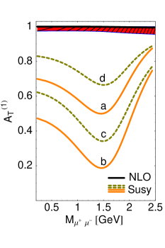
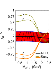
Figure 2: $A_{T}^{(1,2)}(s)$ asymmetries versus the dimuon mass. Thick line correspond to the SM NLO result, while the band around the thick line is the result of adding all errors in quadrature. Curves “a”,“b”,“c” and “d” correspond to specific choice of parameter space in supersymmetry as explained in the text.

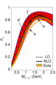
Figure 3: $F_{L}$ versus the dimuon mass. Same conventions ad in Fig. 2.

5 Results

The main results are shown in Figs. 2 and 3, where the asymmetries $A_{T}^{(1)}(s)$ and $A_{T}^{(2)}(s)$ and the polarization fraction $F_{L}(s)$ are shown as a function of the dimuon mass in the SM and in the presence of new physics originating from a MSSM, as described in Section 2.

Let us now discuss those three observables in full detail. First, concerning the SM prediction, and in order to be conservative we have introduced, in addition to the uncertainties discussed in [13], a set of extra parameters, one for each spin amplitude, to explore what the effect of a possible $\Lambda/m_{b}$ correction could be:

$$A_{\bot,\|,0}=A_{\bot,\|,0}^{0}\left(1+c_{\bot,\|,0}\right)$$

where the ‘0’ superscript stands for the QCD NLO Factorisation amplitude and $c_{\bot,\|,0}$ are taken to vary in a range $\pm 10\%$. Note that the transversity amplitudes defined in Eqs. (7)–(9) correspond to physical transitions; hence the combined effect of any power correction is described by a single effective parameter for each of these amplitudes whose size we assumed to be of order $O(10\%)$. It was recently pointed out [42] the existence of a class of power corrections that were taken based on dimensional arguments to be of order $\frac{C_{2}}{3C_{7}}\frac{\Lambda}{m_{b}}\sim\frac{\Lambda}{m_{b}}$ and contribute at leading order to the asymmetries we consider. On the one hand, we note that these corrections just give a contribution to the effective parameters that we introduced; on the other one, we point out that an attempt to estimate these corrections using light-cone QCD sum rules [58, 59] found that they are indeed suppressed by a factor 12 with respect to the dimensional arguments. For these reasons we think that the naive $10\%$ estimate is fair.

Therefore, we allowed these extra parameters to vary independently in a range of $\pm 10\%$ (i.e. a 20% range) for each spin amplitude. The obtained uncertainty was added in quadrature to all other QCD uncertainties (mainly $m_{c}/m_{b}$, scale $\mu$, $f_{B}$, $f_{K}*$, $\lambda_{B,+}$ and $\xi_{\perp}(0)$) and corresponds to the red region in Figs. 2 and 3. It is clear that while the impact on $A^{(1)}_{{T}}({s})$ is very small, $A^{(2)}_{{T}}({s})$ and $F_{L}(s)$ are more affected. Yet, as explained in the following, while the impact on $F_{L}(s)$ turns out to be dramatic when distinguishing new physics, it is not the case for $A^{(2)}_{{T}}({s})$. Notice that the main source of error in $A^{(1,2)}_{{T}}({s})$ shown in Figs. 2 comes from this extra $\pm 10\%$ uncertainty and that all other sources are completely negligible as was found in [13]. This is not the case of $F_{L}(s)$ (see Fig. 3), where the size of the other QCD uncertainties is comparable to this extra uncertainty on the power corrections.

Concerning new physics that come mainly into play via the Wilson coefficient ${C_{7}^{\rm{eff}}}^{\prime}$, the fact that ${C_{7}^{\rm{eff}}}^{\prime}$ does not interfere with $C_{7}^{\rm eff}$ implies that the experimental constraint on the new-physics contributions to ${C_{7}^{\rm{eff}}}^{\prime}$ is much looser than the corresponding one on $C_{7}^{\rm eff}$. Moreover, it is clear from the discussion in Sec. 2, that a non-vanishing ${C_{7}^{\rm{eff}}}^{\prime}$ induces asymmetries already at the LL level. In fact, in the numerical analysis we find large deviations from the SM only if ${C_{7}^{\rm{eff}}}^{\prime}$ is non-zero. This make of those asymmetries a prominent test of right-handed currents.

In order to see if a specific model, MSSM with R-parity conservation and non-minimal flavour changing, can lead naturally to substantial deviations from the SM predictions we have tried to be as generic as possible. We have explored the space of parameters of this supersymmetric model in two separate regions (scenarios A and B) defined by $m_{\tilde{g}}/m_{\tilde{d}}$ being larger (A) and smaller (B) than 1. We have chosen few representative curves of the two different scenarios, to show examples of input parameters, but the whole region between those representative curves and the SM are filled by solutions consistent with all constraints. In both scenarios we take $m^{2}_{u,LL}=m^{2}_{d,LL}=m^{2}_{d,RR}=m_{\tilde{d}}^{2}{\mathbf{1}}_{3\times 3}$, $m^{2}_{u,RR}=m_{\tilde{u}_{R}}^{2}{\mathbf{1}}_{3\times 3}$. $\tan\beta=5$, $\mu=M_{1}=M_{2}=M_{H^{+}}=m_{\tilde{u}_{R}}=1\;{\rm TeV}$. Note that we choose a low value for $\tan\beta$; this shows that we do not need to rely on a large-$\tan\beta$ to see an effect, and ensures automatic fulfillment of the constraint coming from $B_{s}\to\mu^{+}\mu^{-}$.

Moreover, we assume that all the entries in $m^{2}_{u,LR}$ and $m^{2}_{d,LR}$ vanish, with the exception of the one that corresponds to $\left(\delta_{LR}^{d}\right)_{32}$. The remaining parameters are fixed as follows.

• Scenario A: $m_{\tilde{g}}=1\;{\rm TeV}$ and $m_{\tilde{d}}\in[200,1000]\;{\rm GeV}$. The only non-zero mass insertion is varied between $-0.1\leq\left(\delta_{LR}^{d}\right)_{32}\leq 0.1$. For each choice of parameters we first check the list of constraints indicated in the previous section. The curves shown in Figs. 2 and 3, denoted by “a” and “b”, correspond, respectively to $m_{\tilde{g}}/m_{\tilde{d}}=2.5$, $\left(\delta_{LR}^{d}\right)_{32}=0.016$ and $m_{\tilde{g}}/m_{\tilde{d}}=4$, $\left(\delta_{LR}^{d}\right)_{32}=0.036$.

• Scenario B: $m_{\tilde{d}}=1\;{\rm TeV}$ and $m_{\tilde{g}}\in[200,800]\;{\rm GeV}$. The mass insertion is varied in the same range as Scenario A. The curves shown in Figs. 2 and 3 denoted by “c” and “d”, correspond, respectively to $m_{\tilde{g}}/m_{\tilde{d}}=0.7$, $\left(\delta_{LR}^{d}\right)_{32}=-0.01$ and $m_{\tilde{g}}/m_{\tilde{d}}=0.6$, $\left(\delta_{LR}^{d}\right)_{32}=-0.006$.

Interestingly we find that the sign of the asymmetry $A_{T}^{(2)}(s)$ for $m_{\mu^{+}\mu-}<2\;{\rm Gev}$ is anticorrelated with the sign of the mass insertion. The longitudinal polarization fraction $F_{L}(s)$, as anticipated, is poorly sensitive to new physics contributions (already before the inclusion of the uncertainty from $\Lambda/m_{b}$ corrections). The plots in Figs. 2 and 3 have to be compared with the corresponding ones in Figs. 3–8 of Ref. [13].

In Fig. 4, we plot the ratio ${C_{7}^{\rm{eff}}}^{\prime}/\hat{\delta}$ as a function of the common down squark mass $m_{\tilde{d}}$; here $\hat{\delta}=(\delta^{d}_{LR})_{32}/0.005$. The various bands correspond to the different ratios $m_{\tilde{g}}/m_{\tilde{d}}=(0.5,1,2)$. Since we use exact diagonalization of the squark mass matrices, the gluino contribution to ${C_{7}^{\rm{eff}}}^{\prime}$ is not exactly proportional to the mass insertion and we obtain a band rather than a line. The combination of Figs. 1 and 4 allows the immediate translation of a measurement of $A_{T}^{(1,2)}(s)$ into information on $m_{\tilde{g}}$, $m_{\tilde{d}}$ and $(\delta^{d}_{LR})_{32}$ in this framework.

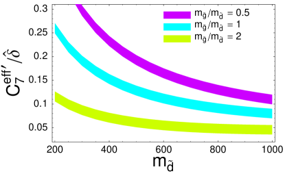
Figure 4: Correlation between ${C_{7}^{\rm{eff}}}^{\prime}/{\hat{\delta}}$ ($\hat{\delta}=(\delta^{d}_{LR})_{32}/0.005$) and $m_{\tilde{d}}$ for various values of $m_{\tilde{g}}/m_{\tilde{d}}$.

6 Conclusions

We have shown that the transverse asymmetries $A_{T}^{(1,2)}(s)$ are an excellent probe of new physics induced by right-handed currents. We considered a minimal supersymmetric model with R-parity conservation and new flavour-changing couplings in the right-handed sector. We found that, after imposing the present experimental constraints, these asymmetries still receive huge enhancements and can be visible at LHCb. The main results are:

• Concerning the SM prediction, we have included an extra set of parameters to mimic a possible contribution coming from the subleading $\Lambda/m_{b}$ correction of order ($\pm 10\%$). We noticed again the robustness of $A_{T}^{(1)}(s)$ and its integrated asymmetry ${\cal A}_{T}^{1}$ compared to $A_{T}^{(2)}(s)$, the integrated ${\cal A}_{T}^{2}$ and $F_{L}(s)$.

• Remarkably, already in the low-$\tan\beta$ regime and taking a very reduced set of parameters ($m_{\tilde{g}}$, $m_{\tilde{d}}$ and $(\delta^{d}_{LR})_{32}$), sizeable effects are found in both asymmetries, large enough to disentangle clearly the supersymmetric contributions of this model from any QCD uncertainty. Notice, moreover, that $A_{T}^{(2)}(s)$ provides information on the sign of the mass insertion. Finally, using the correlation between ${C_{7}^{\rm{eff}}}^{\prime}/\hat{\delta}$ and $m_{\tilde{d}}$ one can obtain information on the three free parameters of this model after a measurement of the asymmetries is done. Concerning the polarization fraction $F_{L}(s)$ we did not find large deviations in any scenario that were not masked by QCD uncertainties.

Negative experimental evidence for deviations in these observables would result in strong constraints on these flavour-changing couplings.

References

- [1]
- [2]
- [3] Y. Nir, arXiv:hep-ph/0109090.
- [4] M. Ciuchini, E. Franco, A. Masiero and L. Silvestrini, J. Korean Phys. Soc. 45 (2004) S223.
- [5] A. J. Buras, arXiv:hep-ph/0505175.
- [6] R. Fleischer, arXiv:hep-ph/0505018.
- [7] T. Hurth, AIP Conf. Proc. 806, 164 (2006).
- [8] T. Feldmann and T. Hurth, JHEP 0411, 037 (2004).
- [9] S. Descotes-Genon, J. Matias and J. Virto, Phys. Rev. Lett. 97, 061801 (2006).
- [10] D. Melikhov, N. Nikitin and S. Simula, Phys. Lett. B 442, 381 (1998).
- [11] C. S. Kim, Y. G. Kim, C.-D. Lü and T. Morozumi, Phys. Rev. D 62, 034013 (2000).
- [12] C. S. Kim, Y. G. Kim and C.-D. Lü, ibid. 64 (2001) 094014.
- [13] F. Kruger and J. Matias, Phys. Rev. D 71, 094009 (2005).
- [14] T. Feldmann and J. Matias, JHEP 0301 (2003) 074.
- [15] J. Matias, Phys. Lett. B 520, 131 (2001).
- [16] F. Krüger, L. M. Sehgal, N. Sinha and R. Sinha, Phys. Rev. D 61, 114028 (2000); 63, 019901(E) (2001).
- [17] P. Ball, J. M. Frère and J. Matias, Nucl. Phys. B 572, 3 (2000).
- [18] P. Colangelo, F. De Fazio, R. Ferrandes and T. N. Pham, Phys. Rev. D 74, 115006 (2006)
- [19] B. Aubert et al. [BABAR Collaboration], Phys. Rev. D 73 (2006) 092001.
- [20] C. Bobeth, M. Misiak and J. Urban, Nucl. Phys. B 567, 153 (2000).
- [21] E. Lunghi, A. Masiero, I. Scimemi and L. Silvestrini, Nucl. Phys. B 568, 120 (2000).
- [22] C. S. Kim, Y. G. Kim and C. D. Lu, Phys. Rev. D 64, 094014 (2001).
- [23] M. Misiak et al., arXiv:hep-ph/0609232.
- [24] M. Misiak and M. Steinhauser, arXiv:hep-ph/0609241.
- [25] S. J. Lee, M. Neubert and G. Paz, arXiv:hep-ph/0609224.
- [26] T. Becher and M. Neubert, arXiv:hep-ph/0610067.
- [27] A. J. Buras and M. Münz, Phys. Rev. D 52, 186 (1995).
- [28] M. Misiak, Nucl. Phys. B393 (1993) 23; B439, 461(E) (1995).
- [29] G. Buchalla, A. J. Buras, and M. E. Lautenbacher, Rev. Mod. Phys. 68, 1125 (1996).
- [30] A. J. Buras, in Probing the Standard Model of Particle Interactions, edited by R. Gupta et al. (Elsevier Science B.V., New York, 1999), p. 281, hep-ph/9806471.
- [31] P. Cho and M. Misiak, Phys. Rev. D 49, 5894 (1994).
- [32] C. Greub, A. Ioannisian and D. Wyler, Phys. Lett. B346 (1995) 149.
- [33] F. Borzumati, C. Greub, T. Hurth and D. Wyler, Phys. Rev. D 62, 075005 (2000).
- [34] T. Besmer, C. Greub and T. Hurth, Nucl. Phys. B609 (2001) 359.
- [35] L. Everett, G. L. Kane, S. Rigolin, L.-T. Wang, and T. T. Wang, J. High Energy Phys. 0201, 022 (2002).
- [36] P. Ball and R. Zwicky, Phys. Rev. D 71 (2005) 014029 [arXiv:hep-ph/0412079].
- [37] M. Beneke, T. Feldmann and D. Seidel, Nucl. Phys. B 612, 25 (2001).
- [38] C. Bobeth, M. Misiak and J. Urban, Nucl. Phys. B 574, 291 (2000).
- [39] P. L. Cho and M. Misiak, Phys. Rev. D 49, 5894 (1994).
- [40] D. Atwood, M. Gronau and A. Soni, Phys. Rev. Lett. 79, 185 (1997) [arXiv:hep-ph/9704272].
- [41] D. Atwood and A. Soni, Z. Phys. C 64 (1994) 241 [arXiv:hep-ph/9401347].
- [42] B. Grinstein, Y. Grossman, Z. Ligeti and D. Pirjol, Phys. Rev. D 71, 011504 (2005) [arXiv:hep-ph/0412019].
- [43] Ulrik Egede, private communication.
- [44] B. Aubert et al. [BABAR Collaboration], Phys. Rev. Lett. 93 (2004) 201801 [arXiv:hep-ex/0405082].
- [45] K. S. Babu and C. F. Kolda, Phys. Rev. Lett. 84, 228 (2000).
- [46] C. Hamzaoui, M. Pospelov and M. Toharia, Phys. Rev. D 59, 095005 (1999).
- [47] G. Isidori and A. Retico, JHEP 0111, 001 (2001).
- [48] A. J. Buras, P. H. Chankowski, J. Rosiek and L. Slawianowska, Phys. Lett. B 546, 96 (2002).
- [49] A. J. Buras, P. H. Chankowski, J. Rosiek and L. Slawianowska, Nucl. Phys. B 659, 3 (2003).
- [50] A. Dedes and A. Pilaftsis, Phys. Rev. D 67, 015012 (2003)
- [51] J. Foster, K. i. Okumura and L. Roszkowski, JHEP 0508, 094 (2005).
- [52] S. Heinemeyer, W. Hollik and G. Weiglein, Comput. Phys. Commun. 124, 76 (2000).
- [53] Heavy Flavor Averaging Group (HFAG), arXiv:hep-ex/0603003.
- [54] P. Gambino and M. Misiak, Nucl. Phys. B 611, 338 (2001).
- [55] T. Hurth, E. Lunghi and W. Porod, Nucl. Phys. B 704, 56 (2005).
- [56] A. L. Kagan and M. Neubert, Eur. Phys. J. C 7, 5 (1999) [arXiv:hep-ph/9805303].
- [57] M. Ciuchini, E. Franco, A. Masiero and L. Silvestrini, Phys. Rev. D 67, 075016 (2003). [Erratum-ibid. D 68, 079901 (2003)]
- [58] P. Ball and R. Zwicky, Phys. Lett. B 642, 478 (2006) [arXiv:hep-ph/0609037].
- [59] P. Ball, G. W. Jones and R. Zwicky, Phys. Rev. D 75, 054004 (2007) [arXiv:hep-ph/0612081].