Wilson loops in heavy ion collisions and their calculation in AdS/CFT

Abstract:

Expectation values of Wilson loops define the nonperturbative properties of the hot medium produced in heavy ion collisions that arise in the analysis of both radiative parton energy loss and quarkonium suppression. We use the AdS/CFT correspondence to calculate the expectation values of such Wilson loops in the strongly coupled plasma of ${\cal N}=4$ super Yang-Mills (SYM) theory, allowing for the possibility that the plasma may be moving with some collective flow velocity as is the case in heavy ion collisions. We obtain the ${\cal N}=4$ SYM values of the jet quenching parameter $\hat{q}$, which describes the energy loss of a hard parton in QCD, and of the velocity-dependence of the quark-antiquark screening length for a moving dipole as a function of the angle between its velocity and its orientation. We show that if the quark-gluon plasma is flowing with velocity $v_{f}$ at an angle $\theta$ with respect to the trajectory of a hard parton, the jet quenching parameter $\hat{q}$ is modified by a factor $\gamma_{f}\left(1-v_{f}\,\cos\theta\right)$, and show that this result applies in QCD as in ${\cal N}=4$ SYM. We discuss the relevance of the lessons we are learning from all these calculations to heavy ion collisions at RHIC and at the LHC. Furthermore, we discuss the relation between our results and those obtained in other theories with gravity duals, showing in particular that the ratio between $\hat{q}$ in any two conformal theories with gravity duals is the square root of the ratio of their central charges. This leads us to conjecture that in nonconformal theories $\hat{q}$ defines a quantity that always decreases along renormalization group trajectories and allows us to use our calculation of $\hat{q}$ in ${\cal N}=4$ SYM to make a conjecture for its value in QCD.

1 Introduction

Understanding the implications of data from the Relativistic Heavy Ion Collider (RHIC) poses qualitatively new challenges [1]. The characteristic features of the matter produced at RHIC, namely its large and anisotropic collective flow and its strong interaction with (in fact not so) penetrating hard probes, indicate that the hot matter produced in RHIC collisions must be described by QCD in a regime of strong, and hence nonperturbative, interactions. In this regime, lattice QCD has to date been the prime calculational tool based solely on first principles. On the other hand, analyzing the very same RHIC data on collective flow, jet quenching and other hard probes requires real-time dynamics: the hot fluid produced in heavy ion collisions is exploding rather than static, and jet quenching by definition concerns probes of this fluid which, at least initially, are moving through it at close to the speed of light. Information on real-time dynamics in a strongly interacting quark-gluon plasma from lattice QCD is at present both scarce and indirect. Complementary methods for real-time strong coupling calculations at finite temperature are therefore desirable.

For a class of non-abelian thermal gauge field theories, the AdS/CFT conjecture provides such an alternative [2]. It gives analytic access to the strong coupling regime of finite temperature gauge field theories in the limit of large number of colors ($N_{c}$) by mapping nonperturbative problems at strong coupling onto calculable problems in the supergravity limit of a dual string theory, with the background metric describing a curved five-dimensional anti-deSitter spacetime containing a black hole whose horizon is displaced away from “our” 3+1 dimensional world in the fifth dimension. Information about real-time dynamics within a thermal background can be obtained in this set-up. The best-known example is the calculation of the shear viscosity in several supersymmetric gauge theories [3, 4, 5, 6, 7, 8, 9, 10]. It was found that the dimensionless ratio of the shear viscosity to the entropy density takes on the “universal” [4, 5, 8, 10] value $1/4\pi$ in the large number of colors ($N_{c}$) and large ’t Hooft coupling ($\lambda\equiv g_{\rm YM}^{2}N_{c}$) limit of any gauge theory that admits a holographically dual supergravity description. Although the AdS/CFT correspondence is not directly applicable to QCD, the universality of the result for the shear viscosity and its numerical coincidence with estimates of the same quantity in QCD made by comparing RHIC data with hydrodynamical model analyses [11] have motivated further effort in applying the AdS/CFT conjecture to calculate other quantities which are of interest for the RHIC heavy ion program. This has lead to the calculation of certain diffusion constants [12] and thermal spectral functions [13], as well as to first work [14] towards a dual description of dynamics in heavy ion collisions themselves. More recently, there has been much interest in the AdS/CFT calculation of the jet quenching parameter which controls the description of medium-induced energy loss for relativistic partons in QCD [15, 16, 17, 18, 19, 20, 21, 22] and the drag coefficient which describes the energy loss for heavy quarks in ${\cal N}=4$ supersymmetric Yang-Mills theory [23, 24, 25, 26, 27]. There have also been studies of the stability of heavy quark bound states in a thermal environment [28, 29, 30] with collective motion [30, 31, 32, 33, 34, 35, 36, 37, 38, 39].

The expectation values of Wilson loops contain gauge invariant information about the nonperturbative physics of non-abelian gauge field theories. When evaluated at temperatures above the crossover from hadronic matter to the strongly interacting quark-gluon plasma, they can be related to a number of different quantities which are in turn accessible in heavy ion collision experiments. In Section 2 of this paper, which should be seen as an extended introduction, we review these connections. We review how the expectation value of a particular time-like Wilson loop, proportional to $\exp(-iS)$ for some real $S$, serves to define the potential between a static quark and antiquark in a (perhaps moving) quark-gluon plasma. However, in order to obtain a sensible description of the photo-absorption cross-section in deep inelastic scattering, the Cronin effect in proton-nucleus collisions, and radiative parton energy loss and hence jet quenching in nucleus-nucleus collisions, the expectation value of this Wilson loop must be proportional to $\exp(-S)$ for some real and positive $S$ once the Wilson loop is taken to lie along the lightcone. In Section 3, we present the calculation of the relevant Wilson loops in hot ${\cal N}=4$ supersymmetric Yang-Mills theory, using the AdS/CFT correspondence, and show how its expectation value goes from $\exp(-iS)$ to $\exp(-S)$ (as it must if this theory is viable as a model for the quark-gluon plasma in QCD) as the order of two non-commuting limits is exchanged. The jet quenching parameter $\hat{q}$, which describes the energy loss of a hard parton in QCD, and the velocity-dependent quark-antiquark potential for a dipole moving through the quark-gluon plasma arise in different limits of the same Nambu-Goto action which depends on the dipole rapidity $\eta$ and on $\Lambda$, the location in $r$, the fifth dimension of the AdS space, of the boundary of the AdS space where the dipole is located. If we take $\eta\to\infty$ first, and only then take $\Lambda\to\infty$, the Nambu-Goto action describes a space-like world sheet bounded by a light-like Wilson loop at $r=\Lambda$, and defines the jet quenching parameter. If instead we take $\Lambda\to\infty$ first, the action describes a time-like world sheet bounded by a time-like Wilson loop, and defines the $q\bar{q}$-potential for a dipole moving with rapidity $\eta$. We review the calculation of both quantities. In Section 4 we calculate the jet quenching parameter in a moving quark-gluon plasma, and show that our result in this section is valid in QCD as in ${\cal N}=4$ SYM. In Section 5 we return to the velocity-dependent screening length, calculating it for all values of the angle between the velocity and orientation of the quark-antiquark dipole.

Section 6 consists of an extended discussion. We summarize our results on the velocity-dependent screening length in Section 6.1. In Section 6.2, we comment on the differences between the calculation of the jet quenching parameter and the drag force on a (heavy) quark [23, 24, 25, 26, 27]. In Section 6.3, we then compare our calculation of the jet quenching parameter to the value of this quantity extracted in comparison with RHIC data. The success of this comparison motivates us to, in Section 6.4, enumerate the differences between QCD and ${\cal N}=4$ supersymmetric Yang-Mills (SYM) theory, which have qualitatively distinct vacuum properties, and the rapidly growing list of similarities between the properties of the quark-gluon plasmas in these two theories. A comparison between our result for the velocity scaling of the quark-antiquark screening length and future data from RHIC and the LHC on the suppression of high transverse momentum $J/\Psi$ and $\Upsilon$ mesons could add one more entry to this list. The single difference between ${\cal N}=4$ SYM and QCD which appears to us most likely to affect the value of the jet quenching parameter is the difference in the number of degrees of freedom in the two theories. We therefore close in Section 6.5 by reviewing the AdS/CFT calculations to date of $\hat{q}$ in theories other than ${\cal N}=4$ SYM, and show that for any two conformal field theories in which this calculation can be done, the ratio of $\hat{q}$ in one theory to that in the other will be given by the square root of the ratio of the central charges, and hence the number of degrees of freedom. This suggests that $\hat{q}$ in QCD is smaller than that in ${\cal N}=4$ SYM by a factor of order $\sqrt{120/47.5}\sim 1.6$. This conjecture can be tested by further calculations in nonconformal theories.

A reader interested in our results and our perspective on our results should focus on Sections 4 and 6. A reader interested in how we obtain our results should focus on Section 3.

2 Wilson loops in heavy ion collisions

In this section, we consider Wilson lines

$$W^{r}({\cal C})={\rm Tr}\,{\cal P}\exp\left[i\int_{\cal C}dx_{\mu}\,A^{\mu}(x)\right]\,,$$ (1)

where $\int_{\cal C}$ denotes a line integral along the closed path ${\cal C}$. $W^{r}({\cal C})$ is the trace of an $SU(N)$-matrix in the fundamental or adjoint representation, $r=F,A$, respectively. The vector potential $A^{\mu}(x)=A^{\mu}_{a}(x)\,T^{a}$ can be expressed in terms of the generators $T^{a}$ of the corresponding representation, and ${\cal P}$ denotes path ordering. We discuss several cases in which nonperturbative properties of interest in heavy ion physics and high energy QCD can be expressed in terms of expectation values of (1).

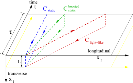
Figure 1: Schematic illustration of the shape of Wilson loops ${\cal C}$, corresponding to a $q\bar{q}$ dipole of size $L$, oriented along the $x_{1}$-direction, which is (i) at rest with respect to the medium (${\cal C}_{\rm static}$), (ii) moving with some finite velocity $v=\tanh\eta$ along the longitudinal $x_{3}$-direction (${\cal C}_{\rm static}^{\rm boosted}$), or (iii) moving with the velocity of light along the $x_{3}$-direction (${\cal C}_{\rm light-like}$).

2.1 The quark-antiquark static potential

We shall use the Wilson loop

$$\langle W^{F}({\cal C}_{\rm static})\rangle=\exp\left[-i\,{\cal T}\,\left(E(L)-E_{\rm ren}\right)\right]$$ (2)

to furnish a working definition of the $q\bar{q}$ static potential $E(L)$ for an infinitely heavy quark-antiquark pair at rest with respect to the medium and separated by a distance $L$. Here, the closed contour ${\cal C}_{\rm static}$ has a short segment of length $L$ in the transverse direction, and a very long extension ${\cal T}$ in the temporal direction, see Fig. 1. The potential $E(L)$ is defined in the limit ${\cal T}\to\infty$. The properties of the medium, including for example its temperature $T$, enter into (2) via the expectation value $\langle\ldots\rangle$. Here, $E_{\rm ren}$ is an $L$-independent renormalization, which is typically infinite. Eq. (2) is written for a Minkowski metric, as appropriate for our consideration, below, of a quark-antiquark pair moving through the medium. At zero temperature, the analytic continuation $i{\cal T}\,\to{\cal T}$ of (2) yields the standard relation between the static potential and an Euclidean Wilson loop [40]. In finite temperature lattice QCD [41, 42, 43], one typically defines a quark-antiquark static potential from the correlation function of a pair of Polyakov loops wrapped around the periodic Euclidean time direction. (For a discussion of this procedure and alternatives to it, see also Ref. [44].) In these Euclidean finite temperature lattice calculations, the corresponding quark-antiquark potential is renormalized such that it matches the zero temperature result at small distances [43]. We shall use an analogous prescription. We note that while (2) is difficult to analyze in QCD, its evaluation is straightforward for a class of strongly interacting gauge theories in the large number of colors limit at both zero [45] and nonzero temperature [28], as we shall see in Section 3.

The dissociation of charmonium and bottomonium bound states has been proposed as a signal for the formation of a hot and deconfined quark-gluon plasma [46]. Recent analyses of this phenomenon are based on the study of the quark-antiquark static potential extracted from lattice QCD [47]. In these calculations of $E(L)$, the $q\bar{q}$-dipole is taken to be at rest in the thermal medium, and its temperature dependence is studied in detail. In heavy ion collisions, however, quarkonium bound states are produced moving with some velocity $v=\tanh\eta$ with respect to the medium. If the relative velocity of the quarkonium exceeds a typical thermal velocity, one may expect that quarkonium suppression is enhanced compared to thermal dissociation in a heat bath at rest [31]. For a calculation of the velocity-dependent dissociation of such a moving $q\bar{q}$-pair in a medium at rest in the $x_{3}$-direction, one has to evaluate (2) for the Wilson loop ${\cal C}_{\rm static}^{\rm boosted}$, depicted in Fig. 1. The orientation of the loop in the $(x_{3},t)$-plane changes as a function of $\eta$. This case is discussed in section 3.1. In section 5, we discuss the generalization to dipoles oriented in an arbitrary direction in the $(x_{1},x_{3})$-plane.

2.2 Eikonal propagation

We now recall cases of physical interest where, unlike in (2), the expectation value of a Wilson loop in Minkowski space is the exponent of a real quantity. Such cases are important in the high energy limit of various scattering problems. Straight light-like Wilson lines of the form $W({\bf x}_{i})={\cal P}\exp\{i\int dz^{-}T^{a}A^{+}_{a}({\bf x}_{i},z^{-})\}$ typically arise in such calculations when — due to Lorentz contraction — the transverse position of a colored projectile does not change while propagating through the target. The interaction of the projectile wave function with the target can then be described in the eikonal approximation as a color rotation $\alpha_{i}\to\beta_{i}$ of each projectile component $i$, resulting in an eikonal phase $W_{\alpha_{i}\beta_{i}}({\bf x}_{i})$. A general discussion of this eikonal propagation approximation can be found in Refs. [48, 49]. Here, we describe two specific cases, in which expectation values of a fundamental and of an adjoint Wilson loop arise, respectively.

2.2.1 Virtual photoabsorption cross section

In deep inelastic scattering (DIS), a virtual photon $\gamma^{*}$ interacts with a hadronic target. At small Bjorken $x$, DIS can be formulated by starting from the decomposition of the virtual photon into hadronic Fock states and propagating these Fock states in the eikonal approximation through the target [50, 51, 52, 53, 54]. However, in a DIS scattering experiment the virtual photon does not have time to branch into Fock states containing many soft particles (equivalently, it does not have time to develop a colored field) prior to interaction, as it would if it could propagate forever. Instead, the dominant component of its wave function which interacts with the target is its $q\bar{q}$ Fock component:

$$|\gamma^{*}\rangle=\int d^{2}({\bf x-y})\,dz\,\psi({\bf x-y},z)\frac{1}{\sqrt{N}}\delta_{\alpha\,\bar{\alpha}}|\alpha({\bf x})\,,\bar{\alpha}({\bf y}),z\rangle\,.$$ (3)

Here, $|\alpha({\bf x})\,,\bar{\alpha}({\bf y}),z\rangle$ denotes a $q\bar{q}$-state, where a quark of color $\alpha$ carries an energy fraction $z$ and propagates at transverse position ${\bf x}$. The corresponding antiquark propagates at transverse position ${\bf y}$ and carries the remaining energy. The Kronecker $\delta_{\alpha\,\bar{\alpha}}$ ensures that this state is in a color singlet. $N$ is the number of colors; the probability that the photon splits into a quark antiquark pair with any one particular color is proportional to $1/N$. The wave function $\psi$ is written in the mixed representation, using configuration space in the transverse direction and momentum space in the longitudinal direction. It can be calculated perturbatively from the $\gamma^{*}\to q\bar{q}$ splitting [53]. Given an incoming state $|\Psi_{\rm in}\rangle=|\alpha({\bf x})\,,\bar{\alpha}({\bf y})\rangle$, in the eikonal approximation the outgoing state reads $|\Psi_{\rm out}\rangle=W_{\alpha\gamma}^{F}({\bf x})\,W_{\bar{\alpha}\bar{\gamma}}^{F\dagger}({\bf y})|\gamma({\bf x})\,,\bar{\gamma}({\bf y})\rangle$, and the total cross section is obtained by squaring $|\Psi_{\rm tot}\rangle=|\Psi_{\rm out}\rangle-|\Psi_{\rm in}\rangle$. From the virtual photon state (3), one finds in this way the total virtual photoabsorption cross section [48]

$$\sigma^{DIS} = \int d^{2}{\bf x}\,d^{2}{\bf y}\,dz\,\psi({\bf x-y},z)\,\psi^{*}({\bf x-y},z)\,P^{q\bar{q}}_{\rm tot}({\bf x},{\bf y})\,,$$ (4)

$$P_{\rm tot}^{q\bar{q}} = \,\left\langle 2-\frac{1}{N}{\rm Tr}\left[W^{F}({\bf x})\,W^{F\dagger}({\bf y})\right]-\frac{1}{N}{\rm Tr}\left[W^{F}({\bf y})\,W^{F\dagger}({\bf x})\right]\right\rangle\,.$$ (5)

This DIS total cross section is written in terms of the expectation value of a fundamental Wilson loop:

$$\frac{1}{N}\langle{\rm Tr}\left[W^{F\,\dagger}({\bf y})\,W^{F}({\bf x})\right]\rangle\longrightarrow\left\langle{W^{F}({\cal C}_{\rm light-like})}\right\rangle=\exp\left[-\frac{1}{8}Q_{s}^{2}\,L^{2}\right]+{\cal O}\left(\frac{1}{N^{2}}\right)\,.$$ (6)

By the $\rightarrow$ we mean that in order to obtain a gauge-invariant formulation, we have connected the two long light-like Wilson lines separated by the small transverse separation $L=|{\bf x}-{\bf y}|$ by two short transverse segments of length $L$, located a long distance $L^{-}\gg L$ apart. This yields the closed rectangular loop ${\cal C}_{\rm light-like}$ illustrated in Fig. 1. The expectation value $\langle\dots\rangle$ denotes an average over the states of the hadronic target; technically, this amounts to an average over the target color fields $A^{\mu}$ in the Wilson line (1). If we could do deep inelastic scattering off a droplet of quark-gluon plasma, the $\langle\dots\rangle$ would be a thermal expectation value. We have parameterized $\langle{W^{F}({\cal C}_{\rm light-like})}\rangle$ in terms of the saturation scale $Q_{s}^{2}$. This is the standard parametrization of virtual photoabsorption cross sections in the saturation physics approach to DIS off hadrons and nuclei [55, 56, 57]. Although we do not know the form of the $1/N^{2}$ corrections to (6), we do know that they must be such that $\langle W^{F}\rangle\rightarrow 0$ in the $L\rightarrow 0$ limit, since in this limit $P_{\rm tot}^{q\bar{q}}$ must vanish.

We note that for small $L$, the $L^{2}$-dependence of the exponent in (6) follows from general considerations. Since the transverse size of the $q\bar{q}$-dipole is conjugate to the virtuality $Q$ of the photon, $L^{2}\sim 1/Q^{2}$, one finds $P_{\rm tot}^{q\bar{q}}=\frac{1}{4}Q_{s}^{2}\,L^{2}+O(L^{4})\sim Q_{s}^{2}/Q^{2}$. This is the expected leading $Q^{2}$-dependence at high virtuality.

General considerations also indicate that the exponent in (6) must have a real part. To see this, consider the limit of large $L$ and small virtuality, when the virtual photon is large in transverse space, and its local interaction probability should go to unity. Since Eq. (5) is the sum of the elastic and inelastic scattering probability, which are both normalized to one, one requires $P_{\rm tot}^{q\bar{q}}\to 2$ in this large-$L$ limit. This cannot be achieved with an imaginary exponent in (6).

The saturation momentum $Q_{s}$ is a characteristic property of any hadronic target. Qualitatively, the gluon distribution inside the hadronic target is dense (saturated) as seen by virtual photons up to a virtuality $Q_{s}$, but it is dilute as seen at higher virtuality. As a consequence, a virtual photon has a probability of order one for interacting with the target, if — in a configuration space picture — its transverse size is $|{\bf x}-{\bf y}|>1/Q_{s}$, and it has a much smaller probability of interaction for $|{\bf x}-{\bf y}|\ll 1/Q_{s}$. This is the physics behind (4) and (5).

2.2.2 The Cronin effect in proton-nucleus (p-A) collisions

In comparing transverse momentum spectra from proton-nucleus and proton-proton collisions, one finds that in an intermediate transverse momentum range of $p_{T}\sim 1-5$ GeV, the hadronic yield in p-A collisions is enhanced [58]. This so-called Cronin effect is typically understood in terms of the transverse momentum broadening of the incoming partons in the proton projectile, prior to undergoing the hard interaction in which the high-$p_{T}$ parton is produced. On the partonic level, this phenomenon and its energy dependence have been studied by calculating the gluon radiation induced by a single quark in the incoming proton projectile scattering on a target of nuclear size $A$ and corresponding saturation scale $Q_{s}$ [59, 60, 61, 62, 63, 64].

One starts from the incoming wave function $\Psi_{\rm in}^{\alpha}$ of a bare quark $|\alpha({\bf 0})\rangle$, supplemented by the coherent state of quasi-real gluons which build up its Weizsäcker-Williams field $f({\bf x})\propto g\frac{{\bf x}}{{\bf x}^{2}}$. Here, $g$ is the strong coupling constant and ${\bf x}$ and ${\bf 0}$ are the transverse positions of the gluon and parent quark [48]. Suppressing Lorentz and spin indices, one has $\Psi_{\rm in}^{\alpha}=|\alpha({\bf 0})\rangle+\int d{\bf x}\,d\xi\,f({\bf x})\,T_{\alpha\beta}^{b}|\beta({\bf 0});b({\bf x},\xi)\rangle$. The ket $|\beta({\bf 0});b({\bf x},\xi)\rangle$ describes the two-parton state, consisting of a quark with color $\beta$ at transverse position ${\bf 0}$ and a gluon of color $b$ at transverse position ${\bf x}$. In the eikonal approximation, the distribution of the radiated gluon is flat in rapidity $\xi$. The outgoing wave function differs from $\Psi_{\rm in}^{\alpha}$ by color rotation with the phases $W^{F}_{\alpha\beta}$ for quarks and $W^{A}_{bc}$ for the gluons:

$$\Psi_{\rm out}^{\alpha} = W^{F}_{\alpha\,\gamma}({\bf 0})\,|\gamma\rangle+\int d{\bf x}\,f({\bf x})\,T_{\alpha\,\beta}^{b}W_{\beta\,\gamma}^{F}({\bf 0})\,W_{b\,c}^{A}({\bf x})\,|\gamma\,;c({\bf x})\rangle\,.$$ (7)

($\alpha$, $\beta$ and $\gamma$ are fundamental indices; $b$, $c$ and $d$ below are adjoint indices.) To calculate an observable related to an inelastic process, such as the number of gluons $dN_{\rm prod}/d{\bf k}$ produced in the scattering, one first determines the component of the outgoing wave function, which belongs to the subspace orthogonal to the incoming state $|\delta\Psi\rangle=\left[1-|\Psi_{in}\rangle\langle\Psi_{in}|\right]|\Psi_{out}\rangle$. Next, one counts the number of gluons in this state [65, 49]

$$\frac{dN_{\rm prod}}{d{\bf k}}=\frac{1}{N}\sum_{\alpha,d}\left\langle\delta\Psi_{\alpha}|a_{d}^{\dagger}({\bf k})\,a_{d}({\bf k})|\,\delta\Psi_{\alpha}\right\rangle$$

$$\quad=\frac{\alpha_{s}\,C_{F}}{2\pi}\,\int d{\bf x}\,d{\bf y}\,e^{i{\bf k}\cdot({\bf x}-{\bf y})}\frac{{\bf x}\cdot{\bf y}}{{\bf x}^{2}\,{\bf y}^{2}}\frac{1}{N^{2}-1}\,\Bigg{[}\left\langle{\rm Tr}\left[W^{A\,\dagger}({\bf 0})\,W^{A}({\bf 0})\right]\right\rangle-\left\langle{\rm Tr}\left[W^{A\,\dagger}({\bf x})\,W^{A}({\bf 0})\right]\right\rangle$$

$$\qquad\qquad\qquad\qquad-\left\langle{\rm Tr}\left[W^{A\,\dagger}({\bf y})\,W^{A}({\bf 0})\right]\right\rangle+\left\langle{\rm Tr}\left[W^{A\,\dagger}({\bf y})\,W^{A}({\bf x})\right]\right\rangle\Bigg{]}\,.$$ (8)

Here, ${\bf x}$ and ${\bf y}$ denote the transverse positions of the gluon in the amplitude and complex conjugate amplitude. The fundamental Wilson lines $W^{F}({\bf 0})$ at transverse position ${\bf 0}$, which appear in (7), combine into an adjoint Wilson line via the identity $W^{A}_{ab}({\bf 0})=2\,{\rm Tr}\left[W^{F}({\bf 0})T^{a}W^{F\dagger}({\bf 0})T^{b}\right]$. We now see that the only information about the target which enters in (8) is that encoded in the transverse size dependence of the expectation value of two light-like adjoint Wilson lines, which we can again close to form a loop:

$$\frac{1}{N^{2}-1}\left\langle{\rm Tr}\left[W^{A\,\dagger}({\bf y})\,W^{A}({\bf x})\right]\right\rangle\longrightarrow\left\langle{W^{A}({\cal C}_{\rm light-like})}\right\rangle=\exp\left[-\frac{1}{4}Q_{s}^{2}\,L^{2}\right]+{\cal O}\left(\frac{1}{N^{2}}\right).$$ (9)

Consistent with the identity ${\rm Tr}\,W^{A}={\rm Tr}\,W^{F}\,{\rm Tr}\,W^{F}-1$, the parameterization of the expectation values of the adjoint and fundamental Wilson loops in (6) and (9) respectively differs in the large-$N$ limit only by a factor of 2 in the exponent.

Inserting (9) into (8), Fourier transforming the Weizsäcker-Williams factors and doing the integrals, one finds formally

$$\frac{dN_{\rm prod}}{d{\bf k}}=\frac{4\pi}{Q_{s}^{2}}\int d{\bf q}\,\exp\left[-\frac{{\bf q}^{2}}{Q_{s}^{2}}\right]\,\frac{{\bf q}^{2}}{{\bf k}^{2}\left({\bf q}-{\bf k}\right)^{2}}\,.$$ (10)

To interpret this expression, we recall the high energy limit for gluon radiation in single quark-quark scattering. For a transverse momentum transfer ${\bf q}$ between the scattering partners, the spectrum in the gluon transverse momentum ${\bf k}$ is proportional to the so-called Bertsch-Gunion factor $\frac{{\bf q}^{2}}{{\bf k}^{2}\left({\bf q}-{\bf k}\right)^{2}}$. Hence, Eq. (10) indicates that the saturation scale $Q_{s}$ characterizes the average squared transverse momentum ${\bf q}^{2}$ transferred from the hadronic target to the highly energetic partonic projectile. We caution the reader that the integrals in (8) are divergent and that the steps leading to (10) remain formal since they were performed without proper regularization of these integrals. Furthermore, a more refined parametrization of the saturation scale in QCD includes a logarithmic dependence of $Q_{s}$ on the transverse separation $L$. Including this correction allows for a proper regularization [65, 60]. The analysis of (8) is more complicated, but the lesson drawn from (10) remains unchanged: the saturation scale $Q_{s}^{2}$ determines the average squared transverse momentum, transferred from the medium to the projectile.

The dependence of the saturation scale $Q^{2}_{s}$ on nuclear size $A$ is $Q_{s}^{2}\propto A^{1/3}$, i.e., $Q_{s}^{2}$ is linear in the in-medium path-length. According to (10), transverse momentum is accumulated in the hadronic target due to Brownian motion, ${\bf q}^{2}\propto A^{1/3}$. In the discussion of high-energy scattering problems in heavy ion physics, where the in-medium path length depends on the geometry and collective dynamics of the collision region, it has proven advantageous to separate this path-length dependence explicitly [66]

$$Q_{s}^{2}=\hat{q}\,\frac{L^{-}}{\sqrt{2}}\,,$$ (11)

in so doing defining a new parameter $\hat{q}$. Here, we have expressed the longitudinal distance $\Delta z=\frac{L^{-}}{\sqrt{2}}$ in terms of the light-cone distance $L^{-}$. The parameter $\hat{q}$ characterizes the average transverse momentum squared transferred from the target to the projectile per unit longitudinal distance travelled, i.e. per unit path length. Note that $\hat{q}$ is well-defined for arbitrarily large $L^{-}$ in an infinite medium, whereas $Q_{s}^{2}$ diverges linearly with $L^{-}$ and so is appropriate only for a finite system. We shall see in Section 2.3 that, when the expectation value in (9) is evaluated in a hot quark-gluon plasma rather than over the gluonic states of a cold nucleus as above, the quantity $\hat{q}$ governs the energy loss of relativistic partons moving through the quark-gluon plasma. The simpler examples we have introduced here in Section 2.2 motivate the need for a nonperturbative evaluation of the light-like Wilson loop $\left\langle{W({\cal C}_{\rm light-like})}\right\rangle$ in a background corresponding to a hadron or a cold nucleus, as in so doing one could calculate the saturation scale and describe DIS at small $x$ and the Cronin effect. Unfortunately, although hot ${\cal N}=4$ supersymmetric Yang-Mills theory describes a system with many similarities to the quark-gluon plasma in QCD as we shall discuss in Section 6, it does not seem suited to modelling a cold nucleus.

2.3 BDMPS radiative parton energy loss and the jet quenching parameter

In the absence of a medium, a highly energetic parton produced in a hard process decreases its virtuality by multiple parton splitting prior to hadronization. In a heavy ion collision, this perturbative parton shower interferes with additional medium-induced radiation. The resulting interference pattern resolves longitudinal distances in the target  [67, 68, 69]. As a consequence, its description goes beyond the eikonal approximation, in which the entire target acts totally coherently as a single scattering center. As we shall explain now, this refined kinematical description does not involve additional information about the medium beyond that already encoded in the jet quenching parameter $\hat{q}$ that we have already introduced.

In the Baier-Dokshitzer-Mueller-Peigne-Schiff [67] calculation of medium-induced gluon radiation, the radiation amplitude for the medium-modified splitting processes $q\to q\,g$ or $g\to g\,g$ is calculated for the kinematic region

$$E\gg\omega\gg|{\bf k}|,|{\bf q}|\equiv|\sum_{i}{\bf q}_{i}|\gg T\,,\Lambda_{\rm QCD}.$$ (12)

The energy $E$ of the initial hard parton is much larger than the energy $\omega$ of the radiated gluon, which is much larger than the transverse momentum ${\bf k}$ of the radiated gluon or the transverse momentum ${\bf q}$ accumulated due to many scatterings of the projectile inside the target. This ordering is also at the basis of the eikonal approximation. In the BDMPS formalism, however, terms which are subleading in $O(1/E)$ are kept and this allows for a calculation of interference effects. To keep $O(1/E)$-corrections to the phase of scattering amplitudes, one replaces eikonal Wilson lines by the retarded Green’s functions [68, 70, 69]

$$G(x^{-}_{2},{\bf r}_{2};x^{-}_{1},{\bf r}_{1}|p)=\int_{{\bf r}(x^{-}_{1})={\bf r}_{1}}^{{\bf r}(x^{-}_{2})={\bf r}_{2}}{\cal D}{\bf r}(x^{-})\,\exp\left[\frac{ip}{2}\int_{x^{-}_{1}}^{x^{-}_{2}}dx^{-}\,\left(\frac{d{\bf r}(x^{-})}{dx^{-}}\right)^{2}-i\,\int_{x^{-}_{1}}^{x^{-}_{2}}dx^{-}\,A^{+}(x^{-},{\bf r}(x^{-}))\right]\,.$$ (13)

Here, $p$ is the total momentum of the propagating parton, and the color field $A^{+}=A^{+}_{a}\,T^{a}$ is in the representation of the parton. The integration goes over all possible paths ${\bf r}(x^{-})$ in the light-like direction between ${\bf r}_{1}={\bf r}(x_{1}^{-})$ and ${\bf r}_{2}={\bf r}(x_{2}^{-})$. Green’s functions of the form (13) are solutions to the Dirac equation in the spatially extended target color field $A^{+}$ [71, 70, 54]. In the limit of ultra-relativistic momentum $p\to\infty$, Eq. (13) reduces to a Wilson line (1) along an eikonal light-like direction. In the BDMPS formalism, the inclusive energy distribution of gluon radiation from a high energy parton produced within a medium can be written in terms of in-medium expectation values of pairs of Green’s functions of the form (13), one coming from the amplitude and the other coming from the conjugate amplitude. After a lengthy but purely technical calculation, it can be written in the form [69]

$$\omega\frac{dI}{d\omega\,d{\bf k}} = \frac{\alpha_{s}\,C_{R}}{(2\pi)^{2}\,\omega^{2}}\,2{\rm Re}\int_{\xi_{0}}^{\infty}dy_{l}\int_{y_{l}}^{\infty}d\bar{y}_{l}\,\int d{\bf u}\,e^{-i{\bf k}\cdot{\bf u}}\,\exp\left[{-\frac{1}{4}\int_{\bar{y}_{l}}^{\infty}d\xi\,\hat{q}(\xi)\,{\bf u}^{2}}\right]\,$$ (14)

$$\times\frac{\partial}{\partial{\bf y}}\cdot\frac{\partial}{\partial{\bf u}}\,\int_{{\bf y}=0}^{{\bf u}={\bf r}(\bar{y}_{l})}{\cal D}{\bf r}\exp\left[\int_{y_{l}}^{\bar{y}_{l}}d\xi\left(\frac{i\,\omega}{2}\dot{\bf r}^{2}-\frac{1}{4}\hat{q}(\xi){\bf r}^{2}\right)\right]\,.$$

Here, the Casimir operator $C_{R}$ is in the representation of the parent parton. In the configuration space representation used in (14), $\xi_{0}$ is the position at which the initial parton is produced in a hard process and the internal integration variables $y_{l}$ and $\bar{y}_{l}$ denote the longitudinal position at which this initial parton radiates the gluon in the amplitude and complex conjugate amplitude, respectively. (See Refs. [69, 49] for details.) Since all partons propagate with the velocity of light, these longitudinal positions correspond to emission times $y_{l}$, $\bar{y}_{l}$.

In deriving (14) [69, 49], the initial formulation of the $q\to q\,g$ radiation amplitude of course involves Green’s functions (13) in both the fundamental and in the adjoint representation. However, via essentially the same color algebraic identities which allowed us to write the gluon spectrum (8) in terms of expectation values of adjoint Wilson loops only, the result given in (14) has been written in terms of expectation values of adjoint light-like Green’s functions of the form (13) only. These in turn have been written in terms of the same jet quenching parameter $\hat{q}$ defined as in (9) and (11), namely via [49]

$$\left\langle{W^{A}({\cal C}_{\rm light-like})}\right\rangle=\exp\left[-\frac{1}{4\sqrt{2}}\,{\hat{q}}L^{-}\,L^{2}\right]+{\cal O}\left(\frac{1}{N^{2}}\right),$$ (15)

now with the expectation value of the light-like Wilson loop evaluated in a thermal quark-gluon plasma rather than in a cold nucleus. The quantity $\hat{q}(\xi)$ which arises in (14) is the value of $\hat{q}$ at the longitudinal position $\xi$, which changes with increasing $\xi$ as the plasma expands and dilutes. In our analysis of a static medium, $\hat{q}(\xi)=\hat{q}$ is constant.

In QCD, radiative parton energy loss is the dominant energy loss mechanism in the limit in which the initial parton has arbitrarily high energy. To see this, we proceed as follows. Note first that in this high parton energy limit the assumptions (12) underpinning the BDMPS calculation become controlled. And, given the ordering of energy scales in (12), the quark-gluon radiation vertex should be evaluated with coupling constant $\alpha_{s}({\bf k}^{2})$. The distribution of the transverse momenta of the radiated gluon is peaked around ${\bf k}^{2}\sim Q_{s}^{2}={\hat{q}}L^{-}/\sqrt{2}$ [72] which means that, in the limit of large in-medium path length $L^{-}/\sqrt{2}$, the coupling $\alpha_{s}$ is evaluated at a scale ${\bf k}^{2}\gg T^{2}$ at which it is weak, justifying the perturbative BDMPS formulation [67]. Next, we note that in the limit of large in-medium path length the result (14) yields [67, 73]

$$\omega\frac{dI}{d\omega}=\frac{\alpha_{s}C_{R}}{\pi}2\,{\rm Re}\,\ln\left[\cos\left((1+i)\,\sqrt{\frac{\hat{q}\,{L^{-}}^{2}/2}{4\omega}}\right)\right]\,.$$ (16)

Integrating this expression over $\omega$, one finds that the average medium-induced parton energy loss is given by

$$\Delta E=\frac{1}{4}\alpha_{s}C_{R}\hat{q}\frac{{L^{-}}^{2}}{2}\ ,$$ (17)

which is independent of $E$ and quadratic in the path length $L^{-}$. This makes the energy lost by gluon radiation parametrically larger in the high energy limit than that lost due to collisions alone, which grows only linearly with path length, and makes radiative energy loss dominant in the high parton energy limit. Radiative parton energy loss has been argued to be the dominant mechanism behind jet quenching at RHIC [68, 69, 75, 76], where the high energy partons whose energy loss is observed in the data have transverse momenta of at most about 20 GeV [1]. At the LHC, the BDMPS calculation will be under better control since the high energy partons used to probe the quark-gluon plasma will then have transverse momenta greater than 100 GeV [77].

Although the BDMPS calculation itself is under control in the high parton energy limit, a weak coupling calculation of the jet quenching parameter $\hat{q}$ is not, as we now explain. Recall that $\hat{q}$ is the transverse momentum squared transferred from the medium to either the initial parton or the radiated gluon, per distance travelled. In a weakly coupled quark-gluon plasma, in which scatterings are rare, $\hat{q}$ is given by the momentum squared transferred in a single collision divided by the mean free path between collisions. Even though the total momentum transferred from the medium to the initial parton and to the radiated gluon is perturbatively large since it grows linearly with the path length, the momentum transferred per individual scattering is only of order $g(T)\,T$. So, a weak-coupling calculation of $\hat{q}$ is justified only if $T$ is so large that physics at the scale $T$ is perturbative. Up to a logarithm, such a weak-coupling calculation yields [67, 66, 78]

$$\hat{q}_{\rm weak-coupling}=\frac{8\zeta(3)}{\pi}\alpha_{s}^{2}N^{2}T^{3}$$ (18)

if $N$, the number of colors, is large. However, given the evidence from RHIC data [1] (the magnitude of jet quenching itself; azimuthal anisotropy comparable to that predicted by zero-viscosity hydrodynamics) that the quark-gluon plasma is strongly interacting at the temperatures accessed in RHIC collisions, there is strong motivation to calculate $\hat{q}$ directly from its definition via the light-like Wilson loop (15), without assuming weak coupling. If and when the quark-gluon plasma is strongly interacting, the coupling constant involved in the multiple soft gluon exchanges described by the weak-coupling calculation of $\hat{q}$ is in fact nonperturbatively large, invalidating (18).

To summarize, the BDMPS analysis of a parton losing energy as it traverses a strongly interacting quark-gluon plasma is under control in the high parton energy limit, with gluon radiation the dominant energy loss mechanism and the basic calculation correctly treated as perturbative. In this limit, application of strong coupling techniques to the entire radiation process described by Eq. (14) would be inappropriate, because QCD is asymptotically free. The physics of the strongly interacting medium itself enters the calculation through the single jet quenching parameter $\hat{q}$, the amount of transverse momentum squared picked up per distance travelled by both the initial parton and the radiated gluon. A perturbative calculation of $\hat{q}$ is not under control, making it worthwhile to investigate any strong coupling techniques available for the evaluation of this one nonperturbative quantity.

3 Wilson loops from AdS/CFT in ${\cal N}=4$ super Yang-Mills theory

In section 2, we have recalled measurements of interest in heavy ion collisions, whose description depends on thermal expectation values of Wilson loops. For questions related to the dissociation of quarkonium, the relevant Wilson loop is time-like and $\langle W({\cal C})\rangle$ is the exponent of an imaginary quantity. Questions related to medium-induced energy loss involve light-like Wilson loops and $\langle W({\cal C})\rangle$ is the exponent of a real quantity.

In this section, we evaluate thermal expectation values of these Wilson loops for thermal ${\cal N}=4$ super Yang-Mills (SYM) theory with gauge group $SU(N)$ in the large $N$ and large ’t Hooft coupling limits, making use of the AdS/CFT correspondence [2, 45]. In the present context, this correspondence maps the evaluation of a Wilson loop in a hot strongly interacting gauge theory plasma onto the much simpler problem of finding the extremal area of a classical string world sheet in a black hole background [28]. We shall find that the cases of real and imaginary exponents correspond to space-like and time-like world sheets, which both arise naturally as we shall describe.

${\cal N}=4$ SYM is a supersymmetric gauge theory with one gauge field $A_{\mu}$, six scalar fields $X^{I},I=1,2,\cdots 6$ and four Weyl fermionic fields $\chi_{i}$, all transforming in the adjoint representation of the gauge group, which we take to be $SU(N)$. The theory is conformally invariant and is specified by two parameters: the rank of the gauge group $N$ and the ’t Hooft coupling $\lambda$,

$$\lambda=g_{YM}^{2}\,N\,.$$ (19)

(Note that the gauge coupling in the standard field theoretical convention $g_{YM}$, which we shall use throughout, is related to that in the standard string theory convention $g_{M}$ by $g_{YM}^{2}=2\,g_{M}^{2}$.)

According to the AdS/CFT correspondence, Type IIB string theory in an $AdS_{5}\times S_{5}$ spacetime is equivalent to an ${\cal N}=4$ SYM living on the boundary of the AdS₅. The string coupling $g_{s}$, the curvature radius $R$ of the AdS metric and the tension $\frac{1}{2\pi\alpha^{\prime}}$ of the string are related to the field theoretic quantities as

$$\frac{R^{2}}{\alpha^{\prime}}=\sqrt{\lambda}\,,\qquad 4\pi\,g_{s}=g_{YM}^{2}=\frac{\lambda}{N}\,.$$ (20)

Upon first taking the large $N$ limit at fixed $\lambda$ (which means $g_{s}\rightarrow 0$) and then taking the large $\lambda$ limit (which means large string tension) ${\cal N}=4$ SYM theory is described by classical supergravity in $AdS_{5}\times S_{5}$. We shall describe the modification of this spacetime which corresponds to introducing a nonzero temperature in the gauge theory below.

${\cal N}=4$ SYM does not contain any fields in the fundamental representation of the gauge group. To construct the Wilson loop describing the phase associated with a particle in the fundamental representation, we introduce a probe D3-brane at the boundary of the AdS₅ and lying along $\vec{n}$ on $S^{5}$, where $\vec{n}$ is a unit vector in ${\bf R}^{6}$ [45]. The D3-brane (i.e. the boundary of the AdS₅) is at some fixed, large value of $r$, where $r$ is the coordinate of the 5th dimension of AdS₅, meaning that the space-time within the D3-brane is ordinary $3+1$-dimensional Minkowski space. The fundamental “quarks” are then given by the ground states of strings originating on the boundary D3-brane and extending towards the center of the AdS₅. The corresponding Wilson loop operator has the form

$$W({\cal C})={1\over N}{\rm Tr}P\exp\left[i\oint_{{\cal C}}ds\,\left(A_{\mu}\dot{x}^{\mu}+\vec{n}\cdot\vec{X}\sqrt{\dot{x}^{2}}\right)\right]$$ (21)

which, in comparison with (1), also contains scalar fields $\vec{X}=(X^{1},\cdots X^{6})$. In the large $N$ and large $\lambda$ limits, the expectation value of a Wilson loop operator (21) is given by the classical action of a string in $AdS_{5}\times S_{5}$, with the boundary condition that the string world sheet ends on the curve ${\cal C}$ in the probe brane. The contour ${\cal C}$ lives within the $3+1$-dimensional Minkowski space defined by the D3-brane, but the string world sheet attached to it hangs “down” into the bulk of the curved five-dimensional AdS₅ spacetime. The classical string action is obtained by extremizing the Nambu-Goto action. More explicitly, parameterizing the two-dimensional world sheet by the coordinates $\sigma^{\alpha}=(\tau,\sigma)$, the location of the string world sheet in the five-dimensional spacetime with coordinates $x^{\mu}$ is

$$x^{\mu}=x^{\mu}(\tau,\sigma)\,,$$ (22)

and the Nambu-Goto action for the string world sheet is given by

$$S=-\frac{1}{2\pi\alpha^{\prime}}\int d\sigma d\tau\,\sqrt{-{\rm det}g_{\alpha\beta}}\,.$$ (23)

Here,

$$g_{\alpha\beta}=G_{\mu\nu}\partial_{\alpha}x^{\mu}\partial_{\beta}x^{\nu}\,$$ (24)

is the induced metric on the world sheet and $G_{\mu\nu}$ is the metric of the $4+1$-dimensional AdS₅ spacetime. The action (23) is invariant under coordinate changes of $\sigma^{\alpha}$. This will allow us to pick world sheet coordinates $(\tau,\sigma)$ differently for convenience in different calculations. Upon denoting the action of the surface which is bounded by ${\cal C}$ and extremizes the Nambu-Goto action (23) by $S({\cal C})$, the expectation value of the Wilson loop (21) is given by [45]

$$\langle{W({\cal C})}\rangle=\exp\left[i\,\{S({\cal C})-S_{0}\}\right]\,,$$ (25)

where the subtraction $S_{0}$ is the action of two disjoint strings, as we shall discuss in detail below.

To evaluate the expectation value of a Wilson loop at nonzero temperature in the gauge theory, one replaces AdS₅ by an AdS Schwarzschild black hole [80]. The metric of the AdS black hole background is given by

$$ds^{2} = -fdt^{2}+\frac{r^{2}}{R^{2}}(dx_{1}^{2}+dx_{2}^{2}+dx_{3}^{2})+\frac{1}{f}dr^{2}=G_{\mu\nu}dx^{\mu}dx^{\nu}\,,$$ (26)

$$f \equiv \frac{r^{2}}{R^{2}}\left(1-\frac{r_{0}^{4}}{r^{4}}\right)\,.$$ (27)

Here, $r$ is the coordinate of the 5th dimension and the black hole horizon is at $r=r_{0}$. According to the AdS/CFT correspondence, the temperature in the gauge theory is equal to the Hawking temperature in the AdS black hole, namely

$$T=\frac{r_{0}}{\pi R^{2}}\,.$$ (28)

The probe D3-brane at the boundary of the AdS₅ space lies at a fixed $r$ which we denote $r=\Lambda\,r_{0}$. $\Lambda$ can be considered a dimensionless ultraviolet cutoff in the boundary conformal field theory. We shall call the three spatial directions in which the D3-brane is extended $x_{1}$, $x_{2}$, and $x_{3}$. The fundamental “quarks”, which are open strings ending on the probe brane, have a mass proportional to ${\Lambda}$. In order to correctly describe a Wilson loop in the continuum gauge theory, we must remove the ultraviolet cutoff by taking the $\Lambda\rightarrow\infty$ limit.

Now consider the set of rectangular Wilson loops shown in Fig. 1, with a short side of length $L$ in the $x_{1}$-direction and a long side along a time-like direction in the $t-x_{3}$ plane, which describe a quark-antiquark pair moving along the $x_{3}$ direction with some velocity $v$. Here, $v=0$ corresponds to the loop ${\cal C}_{\rm static}$ in Fig. 1 whereas $0<v<1$ corresponds to ${\cal C}_{\rm static}^{\rm boosted}$ in the figure. To analyze these loops, it is convenient to boost the system to the rest frame $(t^{\prime},x_{3}^{\prime})$ of the quark pair

$$dt = dt^{\prime}\,\cosh\eta-dx_{3}^{\prime}\,\sinh\eta\,,$$ (29)

$$dx_{3} = -dt^{\prime}\,\sinh\eta+dx_{3}^{\prime}\,\cosh\eta\,,$$ (30)

where the rapidity $\eta$ is given by $\tanh\eta=v$. The loop is now static, but the quark-gluon plasma is moving with velocity $v$ in the negative $x_{3}^{\prime}$-direction. This Wilson loop can be used to describe the potential between two heavy quarks moving through the quark-gluon plasma or, equivalently, two heavy quarks at rest in a moving quark-gluon plasma “wind”. In the primed coordinates, the long sides of the Wilson loop lie along $t^{\prime}$ at fixed $x_{3}^{\prime}$. We denote their lengths by ${\cal T}$, which is the proper time of the quark-pair. We assume that ${\cal T}\gg L$, so that the string world sheet attached to the Wilson loop along the contour ${\cal C}$ can be approximated as time-translation invariant. Plugging (29) and (30) into (26) and dropping the primes, we find

$$ds^{2}=-A\,dt^{2}-2B\,dt\,dx_{3}+C\,dx_{3}^{2}+\frac{r^{2}}{R^{2}}\left(dx_{1}^{2}+dx_{2}^{2}\right)+\frac{1}{f}dr^{2}\$$ (31)

with

$$A={r^{2}\over R^{2}}\left(1-{r_{1}^{4}\over r^{4}}\right),\qquad B={r_{1}^{2}r_{2}^{2}\over r^{2}R^{2}},\qquad C={r^{2}\over R^{2}}\left(1+{r_{2}^{4}\over r^{4}}\right)\,,$$ (32)

where

$$r_{1}^{4}=r_{0}^{4}\cosh^{2}\eta,\qquad r_{2}^{4}=r_{0}^{4}\sinh^{2}\eta\,.$$ (33)

To obtain the light-like Wilson loop along the contour ${\cal C}_{\rm light-like}$ in Fig. 1, we must take the $\eta\rightarrow\infty$ limit. We shall see that the $\eta\rightarrow\infty$ limit and the $\Lambda\rightarrow\infty$ limit do not commute. And, we shall discover that in order to have a sensible phenomenology, we must reach the light-like Wilson loop by first taking the light-like limit ($\eta\rightarrow\infty$) and only then taking the Wilson loop limit ($\Lambda\rightarrow\infty$). For the present, we keep both $\eta$ and $\Lambda$ finite.

We parameterize the two-dimensional world sheet (22), using the coordinates

$$\tau=t,\qquad\sigma=x_{1}\in[-{L\over 2},{L\over 2}]\ .$$ (34)

By symmetry, we will take $x^{\mu}$ to be functions of $\sigma$ only and we set

$$x_{2}(\sigma)={\rm const}\,,\qquad x_{3}(\sigma)={\rm const}\,,\qquad r=r(\sigma)\,.$$ (35)

The Nambu-Goto action (23) now reads

$$S = {{\cal T}\over 2\pi\alpha^{\prime}}\int_{-{L\over 2}}^{{L\over 2}}d\sigma\,\sqrt{A\left({(\partial_{\sigma}r)^{2}\over f}+{r^{2}\over R^{2}}\right)}\ ,$$ (36)

with the boundary condition $r(\pm{L\over 2})=r_{0}{\Lambda}$. This boundary condition ensures that when the string world sheet ends on the D3-brane located at $r=r_{0}\Lambda$, it does so on the contour ${\cal C}$ which is located at $x_{1}=\pm{L\over 2}$. Our task is to find $r(\sigma)$, the shape of the string world sheet hanging “downward in $r$” from its endpoints at $r=r_{0}\Lambda$, by extremizing (36). Introducing dimensionless variables

$$r=r_{0}y,\qquad\tilde{\sigma}=\sigma{r_{0}\over R^{2}},\qquad l={Lr_{0}\over R^{2}}=\pi LT,$$ (37)

where $T$ is the temperature (28), we find that, upon dropping the tilde,

$$S({\cal C})={\sqrt{\lambda}{\cal T}T}\int_{0}^{l\over 2}d\sigma\;{\cal L}\,$$ (38)

with ($y^{\prime}=\partial_{\sigma}y$)

$${\cal L}=\sqrt{\left(y^{4}-{\cosh^{2}\eta}\right)\left(1+{y^{\prime 2}\over y^{4}-1}\right)}$$ (39)

and the boundary condition $y\left(\pm{l\over 2}\right)={\Lambda}$. In writing (38) we have used the fact that, by symmetry, $y({\sigma})$ is an even function. It is manifest from (38) that all physical quantities only depend on $T$ and not on $R$ or $r_{0}$ separately. We must now determine $y(\sigma)$ by extremizing (39). This can be thought of as a classical mechanics problem, with $\sigma$ the analogue of time. Since ${\cal L}$ does not depend on ${\sigma}$ explicitly, the corresponding Hamiltonian

$${\cal H}\equiv{\cal L}-y^{\prime}\frac{\partial{\cal L}}{\partial y^{\prime}}={y^{4}-\cosh^{2}\eta\over{\cal L}}={\rm const}$$ (40)

is a constant of the motion in the classical mechanics problem.

It is worth pausing to recall how it is that the calculation of a Wilson loop in a strongly interacting gauge theory has been simplified to a classical mechanics problem. The large-$N$ and large $\lambda$ limits are both crucial. Taking $N\to\infty$ at fixed $\lambda$ corresponds to taking the string coupling to zero, meaning that we can ignore the possibility of loops of string breaking off from the string world sheet. Then, when we furthermore take $\lambda\to\infty$, we are sending the string tension to infinity meaning that we can neglect fluctuations of the string world sheet. Thus, the string world sheet “hanging down” from the contour ${\cal C}$ takes on its classical configuration, without fluctuating or splitting off loops. If the contour ${\cal C}$ is a rectangle with two long sides, meaning that its ends are negligible compared to its middle, then finding this classical configuration is a classical mechanics problem no more difficult than finding the catenary curve describing a chain suspended from two points hanging in a gravitational field, in this case the gravitational field of the AdS Schwarzschild black hole.

Let us now consider keeping $\Lambda$ fixed and $\gg 1$, while increasing $\eta$ from $0$ to $\infty$. We see that the quantity inside the square root in (39) changes sign when $y$ crosses $\sqrt{\cosh\eta}$. The string world sheet is time-like for real ${\cal L}$ (i.e. for $y>\sqrt{\cosh\eta}$) and is space-like for imaginary ${\cal L}$ (i.e. for $y<\sqrt{\cosh\eta}$). Since $y=\Lambda$ at the boundary ${\cal C}$, the signature of the world sheet depends on the relative magnitude of $\sqrt{\cosh\eta}$ and ${\Lambda}$: it is time-like when $\sqrt{\cosh\eta}<\Lambda$ and becomes space-like when $\sqrt{\cosh\eta}>\Lambda$. If the world sheet in (23) is time-like (space-like), the expectation value (25) of the fundamental Wilson loop is the exponent of an imaginary (real) quantity. We shall give a physical interpretation of this behavior in Section 3.3. Here, we explain that this behavior is consistent with all the phenomenology described in Section 2. For $\eta=0$, the Wilson loop defines the static quark-antiquark potential, see (2), and thus should and does correspond to a time-like world sheet. If the quark-pair is not at rest with respect to the medium, but moves with a small velocity $v=\tanh\eta$, one still expects that the quark-pair remains bound and the world-sheet action remains time-like. We shall see, however, that for large enough $\eta$ a bound quark-antiquark state cannot exist. Once we reach $\eta\equiv\infty$, namely the light-like Wilson loop which we saw in Section 2 originates from eikonal propagation in high energy scattering and is relevant to deep inelastic scattering, the Cronin effect, and jet quenching, in order to have a sensible description of these phenomena we see from (15) or equivalently (6) that the expectation value of the Wilson loop must be the exponent of a real quantity. This expectation is met by (39) since the string world sheet is space-like as long as $\sqrt{\cosh\eta}>\Lambda$. This demonstrates that in order to sensibly describe any of the applications of Wilson loops to high energy propagation, including in particular in our nonzero temperature context the calculation of the jet quenching parameter $\hat{q}$, we must take $\eta\to\infty$ first, before taking the $\Lambda\to\infty$ limit.

In subsection 3.1, we shall review the calculation of the quark-antiquark potential and screening length as a function of the velocity $v$. In subsection 3.2, we calculate the jet quenching parameter. And, in subsection 3.3, we return to the distinction between the time-like string world sheet of subsection 3.1 and the space-like string world sheet of subsection 3.2, and give a physical interpretation of this discontinuity.

3.1 Velocity-dependent quark-antiquark potential and screening length

In this subsection we compute the expectation values of Wilson loops for $\sqrt{\cosh\eta}<\Lambda$, from which we extract the velocity-dependent quark-antiquark potential and screening length. At the end of the calculation we take the heavy quark limit ${\Lambda}\to\infty$. In fact, because we are interested in the case $\sqrt{\cosh\eta}<\Lambda$, in this subsection we could safely take $\Lambda\to\infty$ from the beginning. The results reviewed in this subsection were obtained in Refs. [31, 32, 35].

We denote the constant of the motion identified in Eq, (40) by $q$, and rewrite this equation as

$$y^{\prime}={1\over q}\sqrt{(y^{4}-1)(y^{4}-y_{c}^{4})}$$ (41)

with

$$y_{c}^{4}\equiv\cosh^{2}\eta+q^{2}.$$ (42)

Note that $y_{c}^{4}>\cosh^{2}\eta\geq 1$. The extremal string world sheet begins at $\sigma=-\ell/2$ where $y=\Lambda$, and “descends” in $y$ until it reaches a turning point, namely the largest value of $y$ at which $y^{\prime}=0$. It then “ascends” from the turning point to its end point at $\sigma=+\ell/2$ where $y=\Lambda$. By symmetry, the turning point must occur at $\sigma=0$. We see from (41) that in this case, the turning point occurs at $y=y_{c}$ meaning that the extremal surface stretches between $y_{c}$ and $\Lambda$. The integration constant $q$ can then be determined from the equation ${l\over 2}=\int^{l\over 2}_{0}d\sigma$ which, upon using (41), becomes

$${l}={2q}\int_{y_{c}}^{\Lambda}dy\,{1\over\sqrt{(y^{4}-y_{c}^{4})(y^{4}-1)}}\ .$$ (43)

The action for the extremal surface can be found by substituting (41) into (38) and (39),

$$S(l)={\sqrt{\lambda}{\cal T}T}\int_{y_{c}}^{\Lambda}dy\;{y^{4}-\cosh^{2}\eta\over\sqrt{(y^{4}-1)(y^{4}-y_{c}^{4})}}\ .$$ (44)

Equation (44) contains not only the potential between the quark-antiquark pair but also the static mass of the quark and antiquark considered separately in the moving medium. (Recall that we have boosted to the rest frame of the quark and antiquark, meaning that the quark-gluon plasma is moving.) Since we are only interested in the quark-antiquark potential, we need to subtract from (44) the action $S_{0}$ of two independent quarks, namely

$$E(L){\cal T}=S(l)-S_{0}\,,$$ (45)

where $E(L)$ is the quark-antiquark potential in the dipole rest frame. The string configuration corresponding to a single quark at rest in a moving hot medium in ${\cal N}=4$ SYM was found in Refs. [23, 24], from which one finds that

$$S_{0}=\sqrt{\lambda}\,{\cal T}\,T\,\int_{1}^{{\Lambda}}dy\,.$$ (46)

To be self-contained, in appendix A we review the solution of [23, 24], along with a family of new drag solutions describing string configurations corresponding to mesons made from a heavy and a light quark.

Figure 2: Left panel: the quark-antiquark separation $l(q)$ as a function of the integration constant $q$ for a quark-antiquark dipole oriented orthogonal to the wind propagating at different velocities $v=\tanh\eta$. We discuss the case where the dipole is not orthogonal to the wind in Section 5. Right panel: The $q\bar{q}$ static potential for the same quark-antiquark configurations as in the left panel. Note that the potential is normalized such that the small-distance behavior of the potential is unaffected by velocity-dependent medium effects.

To extract the quark-antiquark potential, we use (43) to solve for $q$ in terms of $l$ and then plug the corresponding $q(l)$ into (44) and (45) to obtain $E(L)$. We can safely take the ${\Lambda}\rightarrow\infty$ limit, and do so in all results we present. We show results at a selection of velocities in Fig. 2. In the remainder of this subsection, we describe general features of these results.

First, Eq. (44) has no solution when $l>l_{\rm max}(\eta)$, where $l_{\rm max}$ is the maximum of $l(q)$. We see that $l_{\rm max}$ decreases with increasing velocity.

We see from the left panel in Fig. 2 that for a given $l<l_{\rm max}(\eta)$, there are two branches of solutions. The branch with the bigger value of $q$, and therefore the larger turning point $y_{c}$, has the smaller $E(L)$ — corresponding to the lower branches of each of the curves in the right panel of the figure. The upper branches of each curve correspond to the solutions for a given $l<l_{\rm max}$ with smaller $q$ and $y_{c}$. Because they have higher energy, it is natural to expect that they describe unstable solutions sitting at a saddle point in configuration space [32, 34]. This has been confirmed explicitly in Ref. [36].

When $\eta$ is greater than some critical value $\eta_{c}$, $E(L)$ is negative for the whole upper branch. When $\eta<\eta_{c}$, there exists a value $l_{c}(\eta)<l_{max}$ such that the upper branch has an $E(L)$ which is negative for $l<l_{c}$ and positive for $l>l_{c}$. $l_{c}$ goes to zero as $\eta$ goes to zero. If $\eta<\eta_{c}$ and $l>l_{c}$, then if the unstable upper branch configuration is perturbed, after some time it could settle down either to the lower branch solution or to two isolated strings each described by the drag solution of Ref. [23, 24] and Appendix A. (Note that $E>0$ means that a configuration has more energy than two isolated strings.) On the other hand, if $E(L)$ is negative for the upper branch, when this unstable configuration is perturbed, the only static solution we know of to which it can settle after some time is the lower branch solution.

We see from Fig. 2 that using the action of the dragging string solution of Refs. [23, 24] as $S_{0}$ as we do and as was considered as an option in Ref. [35], ensures that the small-distance behavior of the potential is velocity-independent. This seems to us a physically reasonable subtraction condition; it is analogous to the renormalization criterion used to define the quark-antiquark potential in lattice calculations, namely that at short distances it must be medium-independent [43]. Choosing the velocity-dependent subtraction (144) instead, considered as an option in Ref. [35], makes the unstable upper branch have $\lim_{L\to 0}E(L)=0$ for all velocities, but in so doing makes the stable lower-branch have a velocity-dependent $E(L)$ at all $L$, including small $L$.

One can obtain an analytical expression for $l_{\rm max}$ in the limit of high velocity. Expanding (43) in powers of $1/y_{c}^{4}$ gives

$$l(q)=\frac{2\sqrt{\pi}q}{y_{c}^{3}}\left(\frac{\Gamma\left(\frac{3}{4}\right)}{\Gamma\left(\frac{1}{4}\right)}+\frac{\Gamma\left(\frac{7}{4}\right)}{8\Gamma\left(\frac{9}{4}\right)}\frac{1}{y_{c}^{4}}+\frac{3\Gamma\left(\frac{11}{4}\right)}{32\Gamma\left(\frac{13}{4}\right)}\frac{1}{y_{c}^{8}}+O\left(\frac{1}{y_{c}^{12}}\right)\right)\ .$$ (47)

Truncating this expression after the second term, we find for the maximum

$$l_{\rm max} = \frac{\sqrt{2\pi}\,\Gamma\left(\frac{3}{4}\right)}{3^{3/4}\Gamma\left(\frac{1}{4}\right)}\left(\frac{2}{\cosh^{1/2}\eta}+\frac{1}{5\cosh^{5/2}\eta}+\cdots\right)$$ (48)

$$= 0.74333\left(\frac{1}{\cosh^{1/2}\eta}+\frac{1}{10\,\cosh^{5/2}\eta}+\cdots\right)\ .$$

Note that $L_{max}={l_{max}\over\pi T}$ can be interpreted as the screening length in the medium, beyond which the only solution is the trivial solution corresponding to two disjoint world sheets and thus $E(L)=0$. The first term of this expression was given in [31] (see also [32]), the second term in [35]. As we shall discuss further at the end of Section 5, if we set $\eta=0$ in (48), this expression which was derived for $\eta\rightarrow\infty$ is not too far off the $\eta=0$ result, which is $\ell_{\rm max}=0.869$. Hence, as discovered in Ref. [31], the screening length decreases with increasing velocity to a good approximation according to the scaling

$$L_{\rm max}(v)\simeq\frac{L_{\rm max}(0)}{\cosh^{1/2}\eta}=\frac{L_{\rm max}(0)}{\sqrt{\gamma}},$$ (49)

with $\gamma=1/\sqrt{1-v^{2}}$. This velocity dependence suggests that $L_{s}$ should be thought of as, to a good approximation, proportional to (energy density)^-1/4, since the energy density increases like $\gamma^{2}$ as the wind velocity is boosted.

If the velocity-scaling of $L_{s}$ that we have discovered holds for QCD, it will have qualitative consequences for quarkonium suppression in heavy ion collisions [31]. For illustrative purposes, consider the explanation of the $J/\Psi$ suppression seen at SPS and RHIC energies proposed in Refs. [81, 82]: lattice calculations of the $q\bar{q}$-potential indicate that the $J/\Psi$(1S) state dissociates at a temperature $\sim 2.1T_{c}$ whereas the excited $\chi_{c}$(2P) and $\Psi^{\prime}$(2S) states cannot survive above $\sim 1.2T_{c}$; so, if collisions at both the SPS and RHIC reach temperatures above $1.2T_{c}$ but not above $2.1T_{c}$, the experimental facts (comparable anomalous suppression of $J/\Psi$ production at the SPS and RHIC) can be understood as the complete loss of the “secondary” $J/\Psi$’s that would have arisen from the decays of the excited states, with no suppression at all of $J/\Psi$’s that originate as $J/\Psi$’s. Taking Eq. (49) at face value, the temperature $T_{\rm diss}$ needed to dissociate the $J/\Psi$ decreases $\propto(1-v^{2})^{1/4}$. This indicates that $J/\Psi$ suppression at RHIC may increase markedly (as the $J/\Psi$(1S) mesons themselves dissociate) for $J/\Psi$’s with transverse momentum $p_{T}$ above some threshold that is at most $\sim 9$ GeV and would be $\sim 5$ GeV if the temperatures reached at RHIC are $\sim 1.5T_{c}$. The kinematical range in which this novel quarkonium suppression mechanism is operational lies within experimental reach of future high-luminosity runs at RHIC and will be studied thoroughly at the LHC in both the $J/\Psi$ and Upsilon channels. If the temperature of the medium produced in LHC collisions proves to be large enough that the $J/\Psi$(1S) mesons dissociate already at low $p_{T}$, the $p_{T}$-dependent pattern that the velocity scaling (49) predicts in the $J/\Psi$ channel at RHIC should be visible in the Upsilon channel at the LHC.

As a caveat, we add that in modelling quarkonium production and suppression versus $p_{T}$ in heavy ion collisions, various other effects remain to be quantified. For instance, secondary production mechanisms such as recombination may contribute significantly to the $J/\Psi$ yield at low $p_{T}$, although the understanding of such contributions is currently model-dependent. Also, at very high $p_{T}$, $J/\Psi$ mesons could form outside the hot medium [83]. Parametric estimates of this effect suggest that it is important only at much higher $p_{T}$ than is of interest to us, and we are not aware of model studies which have been done that would allow one to go beyond parametric estimates. The quantitative importance of these and other effects may vary significantly, depending on details of their model implementation. In contrast, Eq. (49) was obtained directly from a field-theoretic calculation and its implementation will not introduce additional model-dependent uncertainties. For this reason, the velocity scaling established here must be included in all future model calculations. We expect that its effect is most prominent at intermediate transverse momentum, where contributions from secondary production die out or can be controlled, while the formation time of the heavy bound states is still short enough to ensure that they would be produced within the medium if the screening by the medium permits.

3.2 Light-like Wilson loop and the jet quenching parameter

In order to calculate the jet quenching parameter we need to take the $\eta\to\infty$ limit in which the Wilson loop becomes light-like first, with the location of the boundary D3-brane $\Lambda$ large and fixed, and only later take $\Lambda\to\infty$. As we approach the light-like limit, it is necessary that $\sqrt{\cosh\eta}>{\Lambda}$. In this regime, as we discussed below equation (40), the world sheet is space-like, meaning that the expectation value of the Wilson loop is the exponential of a real quantity. As we reviewed in Section 2, this must be the case in order to obtain sensible results for both medium-induced gluon radiation of Eq. (8) and the virtual photo-absorption cross section in deep inleastic scattering of Eq. (4).

When $\sqrt{\cosh\eta}>{\Lambda}$, the first order equation of motion, given by (40), reads

$$y^{\prime 2}={1\over q^{2}}(y^{4}-1)(y_{m}^{4}-y^{4})$$ (50)

with

$$y_{m}^{4}=\cosh^{2}\eta-q^{2}\ .$$ (51)

The consistency of (50) requires that $y_{m}>\Lambda$, which implies that the integration constant $q$ is constrained to $0\leq q^{2}\leq\cosh^{2}\eta-{\Lambda}^{4}$. Equation (50) has a trivial solution

$$y({\sigma})=\Lambda={\rm const},\qquad q^{2}=\cosh^{2}\eta-{\Lambda}^{4}\ .$$ (52)

However, one can check that (52) does not solve the second order Euler-Lagrange equation of motion derived from (39) and thus should be discarded. Because $y_{m}>\Lambda$, the nontrivial solution of (50) which descends from $y=\Lambda$ at $\sigma=-l/2$ descends all the way to $y=1$, where $y^{\prime}=0$. Thus, for any value of $l$ the string starts at $y={\Lambda}$ and descends all the way to the horizon, where it turns around and then ascends back up to $y={\Lambda}$. The integration constant $q$ can be determined from the equation ${l\over 2}=\int^{l\over 2}_{0}d\sigma$, i.e

$${l}={2q}\int_{1}^{{\Lambda}}dy\,{1\over\sqrt{(y^{4}_{m}-y^{4})(y^{4}-1)}}\,$$ (53)

upon using (50). The action (36) takes the form

$$S(l)=i{\sqrt{\lambda}{\cal T}T}\int_{1}^{\Lambda}dy\;{\cosh^{2}\eta-y^{4}\over\sqrt{(y^{4}-1)(y_{m}^{4}-y^{4})}}\,.$$ (54)

This action is imaginary and corresponds to a space-like world sheet.

To extract $\hat{q}$ introduced in (6), (11) and (15), we first take $\eta\to\infty$, making the contour ${\cal C}$ light-like, and only then take the $\Lambda\to\infty$ limit needed to ensure that we are evaluating $W({\cal C})$, with the end of the string on the D3-brane at $y=\Lambda$ following the contour ${\cal C}$ precisely. $\hat{q}$ can be obtained by studying the small $l$-dependence of the action (54), which can be done analytically. We start from the expansion of (53),

$${l} = \frac{2q}{\cosh\eta}\int_{1}^{\Lambda}dy\frac{1}{\sqrt{y^{4}-1}}+{\cal O}\left(q^{3},\frac{\Lambda^{4}}{\cosh^{2}\eta}\right)\,.$$ (55)

Upon defining

$$\alpha\equiv\lim_{\Lambda\to\infty}\int_{1}^{\Lambda}dy\frac{1}{\sqrt{y^{4}-1}}=\sqrt{\pi}\frac{\Gamma\left(\frac{5}{4}\right)}{\Gamma\left(\frac{3}{4}\right)}\,,$$ (56)

we find that in the small $l$ (equivalently, small $q$) limit

$$l=\frac{2\alpha q}{\cosh\eta}\ .$$ (57)

In the same limit, the action (54) takes the form

$$S(l)=S^{(0)}+q^{2}S^{(1)}+O(q^{4})\,,$$ (58)

where

$$S^{(0)} = i\sqrt{\lambda}{\cal T}T\int_{1}^{\Lambda}dy\,\sqrt{\cosh^{2}\eta-y^{4}\over y^{4}-1}\,,$$ (59)

$$q^{2}S^{(1)}(l) = \frac{i\sqrt{\lambda}{\cal T}T}{2}q^{2}\int_{1}^{\Lambda}dy\,\frac{1}{\sqrt{\left(\cosh^{2}\eta-y^{4}\right)\left(y^{4}-1\right)}}$$ (60)

$$= \frac{i\sqrt{\lambda}{\cal T}Tq^{2}\alpha}{2\cosh\eta}=i\frac{\sqrt{\lambda}\pi^{2}\,T^{3}}{8\,\alpha}\left({\cal T}\cosh\eta\right)L^{2}\,,$$

where we have used (56), (57) and $l=\pi\,L\,T$. Also, we have kept the dominant large $\eta$-dependence only. We identify $\left({\cal T}\cosh\eta\right)=L^{-}/\sqrt{2}$, where $L^{-}$ is the extension of the Wilson loop in the light-like direction, entering in (11) and (15).

As in Section 3.1, in order to determine the expectation of the Wilson line we need to subtract the action of two independent single quarks, this time moving at the speed of light. In Appendix A, we analyze the string configuration corresponding a single quark moving at the speed of light. There we find a class of solutions with space-like world sheets and also a class of solutions with time-like world sheet. Our criterion to determine which solution to subtract is motivated from the physical expectation discussed in Section 2, i.e.

$$\lim_{l\to 0}\left[S(l)-S_{0}\right]=S^{(0)}-S_{0}=0\,.$$ (61)

Among the classes of solutions discussed in Appendix A, the only one satisfying (61) is the space-like world sheet described by Eqs. (149) and (150) with $p=0$. In this configuration, $S_{0}$ is the action of two straight strings extending from $y={\Lambda}$ to $y=1$ along the radial direction and is given by

$$S_{0}=i\sqrt{\lambda}{\cal T}T\int_{1}^{\Lambda}dy\,\sqrt{\cosh^{2}\eta-y^{4}\over y^{4}-1}\,.$$ (62)

The $L^{2}$-term in the exponent of (15) can then be identified with the $O(L^{2})$-term (60) of the action $S(l)$, and we thus conclude that the jet quenching parameter in (15) is given by

$$\hat{q}_{SYM}=\frac{\pi^{3/2}\Gamma\left(\frac{3}{4}\right)}{\Gamma\left(\frac{5}{4}\right)}\sqrt{\lambda}\,T^{3}\,.$$ (63)

We have used the fact that, as in (9), in the large-$N$ limit the expectation value of the adjoint Wilson loop which defines $\hat{q}$ in (15) differs from that of the fundamental Wilson loop which we have calculated by a factor of 2 in the exponent $S$.

In Ref. [15], the result (63) was obtained starting directly from the loop ${\cal C}_{\rm light-like}$, described in the rest frame of the medium using light-cone coordinates. Here, we showed that one can obtain the same result by taking the $v\to 1$ limit of a time-like Wilson loop. It is also easy to check that the trivial solution (52) goes over to the constant solution discussed in [15], which has a smaller action than (54). In [15] this trivial solution was discarded on physical grounds. Here, we see that if we treat the light-like Wilson line as the $\eta\to\infty$ limit of a time-like one, this trivial solution does not even arise. We also note that in the light-like limit, the coefficient in front of the scalar field term in (21) goes to zero and (21) coincides with (1).

In Section 4 we shall determine how $\hat{q}$ changes if the medium in which the expectation value of the light-like Wilson loop is evaluated has some flow velocity at an arbitrary angle with respect to the direction of the Wilson loop. In Section 6 we shall discuss the comparison between our result for $\hat{q}$ and that extracted by comparison with RHIC data, as well as discuss how $\hat{q}$ changes with the number of degrees of freedom in the theory.

3.3 Discussion: time-like versus space-like world sheets

We have seen that as we increase $\eta$ from $0$ to $\infty$ while keeping ${\Lambda}$ fixed and large, the behavior of the string world sheet has a discontinuity at $\sqrt{\cosh\eta}={\Lambda}$, below (above) which the world sheet is time-like (space-like). Here we give a physical interpretation for this discontinuity. Recall first from Section 3.1 that if $\cosh\eta\gg 1$ but $\sqrt{\cosh\eta}<{\Lambda}$, the screening length $L_{\rm max}$ is given by

$$L_{\rm max}={0.743\over\pi\sqrt{\cosh{\eta}}\,T}\ .$$ (64)

Next, note that the size $\delta$ of our external quark on the D3-brane at $y=\Lambda$, i.e. at $r=r_{0}\Lambda=\pi R^{2}T\Lambda$ can be estimated using the standard IR/UV connection, namely [79]

$$\delta\sim{\sqrt{\lambda}\over M}\sim{1\over{\Lambda}\,T}\ ,$$ (65)

where $M={1\over 2}\sqrt{\lambda}T{\Lambda}$ is the mass of an external quark as can be read from (46). (The apparent $T$-dependence of (65) is due to our definition of ${\Lambda}$, with the ultraviolet cutoff given by ${\Lambda}r_{0}$, and does not reflect genuine temperature-dependence.) Thus the condition $\sqrt{\cosh\eta}={\Lambda}$ corresponds to [32]

$$L_{max}\sim\delta\ .$$ (66)

When $\sqrt{\cosh\eta}\ll{\Lambda}$, meaning that $\delta\ll L_{\rm max}$, we expect that if instead of merely analyzing Wilson loops we were to actually study mesons, we would in fact find a bound state of a quark and anti-quark. In this regime, it is reasonable to expect that the expectation value of the Wilson loop should yield information about the quark-antiquark potential, meaning that it must be the exponential of an imaginary quantity meaning that the string world sheet must be time-like, as indeed we find. On the other hand, when $\sqrt{\cosh\eta}\gg{\Lambda}$, meaning that $\delta\gg L_{\rm max}$, the size of one quark by itself is much greater than the putative screening length. This means that the quark and antiquark cannot bind for any $L$, meaning that the transition at $\sqrt{\cosh\eta}\sim{\Lambda}\sim M/(\sqrt{\lambda}T)$ can be thought of as a “deconfinement” or “dissociation” transition for quarkonium mesons made from quarks with mass $M$. Furthermore, in a regime in which the size of one quark is greater than the putative screening length, the concept of a quark-antiquark potential (and a screening length) makes no sense. Instead, in this regime it is appropriate to think of the quark-antiquark pair as a component of the wave function of a virtual photon in deep inelastic scattering, and hence to think of the Wilson loop as arising in the eikonal approximation to this high energy scattering process, as discussed in Section 2. From our discussion there, it is then natural to expect a space-like world sheet, which gives the desired $\langle W\rangle\sim\exp[-S]$ behavior with $S$ real.

Our discussion explains the qualitative change in physics, but it does not explain the sharpness of the discontinuity that we find at $\sqrt{\cosh\eta}={\Lambda}$, which likely has to do with the classical string approximation (which corresponds to large $N$ and large $\lambda$ limit) we are using. When $\sqrt{\cosh\eta}<{\Lambda}$ there is a discontinuity between $L<L_{\rm max}$ and $L>L_{\rm max}$ where the quark-antiquark potential goes from being nonzero to zero. This discontinuity is smoothed out by finite $\lambda$ corrections, with the exponentially small quark-antiquark potential at large distances corresponding to physics that is nonperturbative in $\alpha^{\prime}$. Presumably the discontinuity at $\sqrt{\cosh\eta}={\Lambda}$ is also smoothed out at finite $\lambda$ and $N$. Further insight into this question could perhaps be obtained without relaxing the large-$N$ and large-$\lambda$ limits by studying mesons rather than Wilson loops.

The operational consequences of the discontinuity at $\sqrt{\cosh\eta}={\Lambda}$ are clear. To compute the quark-antiquark potential and the screening length in a moving medium, we take ${\Lambda}$ to infinity at fixed $\eta$. To compute $\hat{q}$, we must instead first take the $\eta\rightarrow\infty$ limit at finite $\Lambda$, and only then take $\Lambda\rightarrow\infty$. The two limits do not commute.

4 The jet quenching parameter in a flowing medium

In section 3.2, we have evaluated the expectation value of a light-like Wilson loop specified by the trajectory of a dipole moving in a light-like direction, $k^{\mu}=(1,\hat{n})$ with $\hat{n}$ a unit vector and hence $k^{2}=0$. The world sheet defined by this light-like Wilson loop is space-like and the behavior of the Nambu-Goto action in the limit of small dipole size determines the jet quenching parameter $\hat{q}$. It has been argued previously that the motion of the medium orthogonal to the trajectory of the dipole can affect the value of $\hat{q}$ in a nontrivial fashion [84, 85]. Furthermore, if the medium is flowing parallel to or antiparallel to the trajectory of the dipole with velocity $v_{f}=\tanh\eta_{f}$, there is a straightforward effect on $\hat{q}$: the calculation goes through unchanged, with $L^{-}$ understood to be the light-cone distance in the rest frame of the medium, but the relation between $L^{-}$ and the distance $\Delta z$ travelled in the lab frame is modified: $\Delta z=(L^{-}/\sqrt{2})\exp(\eta_{f})$, where the sign convention is such that $\eta_{f}>0$ corresponds to the dipole velocity and flow velocity parallel (i.e. the dipole feels a “tail wind”) while $\eta_{f}<0$ means that the dipole feels a head wind. Correspondingly, $\hat{q}$ is multiplied by a factor of $\exp(-\eta_{f})$, meaning that it increases in a head wind and decreases in a tail wind. In this Section, we calculate how the jet quenching parameter $\hat{q}$ depends on the speed and direction of the collective flow of the medium, allowing for any angle between the jet direction and the flow direction.

The calculation of the effect on jet quenching parameter $\hat{q}$ due to the collective motion of the medium turns out to be straightforward, once the geometry of the problem is set up. We shall specify the light-like four-momentum $k^{\mu}=(1,\hat{n})$ (the direction of motion of the hard parton which is losing energy; the direction of propagation of the dipole moving at the speed of light which defines the Wilson loop) by taking $\hat{n}$ to point along the negative $x_{3}$-direction. According to the way the BDMPS energy loss calculation is set up, the dipole is always perpendicular to the direction of its motion, so we choose the dipole orientation to point in a direction $\hat{m}$ which must lie in the $(x_{1},x_{2})$-plane. Now, we set the medium in motion. The most general “wind velocity” has components parallel to and orthogonal to the dipole direction $\hat{n}$. We choose $\vec{v}=v\hat{l}$ to lie in the $(x_{2},x_{3})$-plane. Because we fix the orthogonal component to lie along the $x_{2}$-direction, we must leave the direction of the dipole orientation $\hat{m}$ in the $(x_{1},x_{2})$-plane unspecified. Thus the most general configuration is described by four parameters, the transverse separation $L$ of the Wilson loop in the lab frame and

$$\cosh\eta_{f}={1\over\sqrt{1-v^{2}}}\,,\qquad\theta=\angle(\hat{l},\hat{n})\,,\qquad\phi=\angle(\hat{m},\vec{x}_{1})\,.$$ (67)

In the lab frame, the trajectory of the end points of the dipole can be written as

$$A^{\mu}_{\pm}=k^{\mu}t\pm{L\over 2}m^{\mu}\,,$$ (68)

where

$$\qquad k^{\mu}=(1,\hat{n}),\qquad m^{\mu}=(0,\hat{m}),\qquad k\cdot m=0,\qquad k^{2}=0,\qquad m^{2}=1\,.$$ (69)

Now, we boost $A^{\mu}$ with $\vec{v}=v\hat{l}$, boosting into a frame in which the medium is at rest. We obtain

$$A^{\prime\mu}_{\pm}=k^{\prime\mu}t\pm{L\over 2}m^{\prime\mu}\,,$$ (70)

for some $k^{\prime\mu}$ and $m^{\prime\mu}$ which again satisfy

$$k^{\prime 2}=0,\qquad m^{\prime 2}=1,\qquad m^{\prime}\cdot k^{\prime}=0\,.$$ (71)

In general, $m^{\prime\mu}$ has a nonzero $0$-th component and thus the two ends of the dipole do not have the same time. To fix this we write

$$A^{\prime\mu}_{\pm}=k^{\prime\mu}(t\pm t_{0})\pm{L\over 2}m^{\prime\prime\mu}\,,$$ (72)

where we have defined

$$m^{\prime\prime\mu}=m^{\prime\mu}-t_{0}k^{\prime\mu}\,,$$ (73)

and choose $t_{0}$ such that the zeroth component of $m^{\prime\prime}$ is zero, making $m"^{\mu}$ purely spatial. It is easy to confirm that, given (72), we now have

$$k^{\prime 2}=0,\qquad m^{\prime\prime 2}=1,\qquad m^{\prime\prime}\cdot k^{\prime}=0\,.$$ (74)

We now have almost exactly the same Wilson loop configuration as we had in our original calculation of Section 3.2 when the medium was at rest from the beginning, with the only difference being that the two long sides of the Wilson loop do not start and end at equal times, due to the shift $t_{0}$. This is immaterial when $L_{-}$ is big: in our evaluation of the Wilson loop we always assumed time translational invariance anyway, neglecting the contribution of the “ends of the loop” relative to that of the long, time translation invariant, mid-section of the loop. We thus find that in the presence of a wind velocity

$$\langle{W^{A}({\cal C})}\rangle=\exp\left[-S({\cal C})\right]$$ (75)

with

$$S({\cal C})=-{1\over 4\sqrt{2}}\hat{q}_{0}(L^{-})^{\prime}L^{2}\,,$$ (76)

where $\hat{q}_{0}$ is the value with no wind and where

$$(L^{-})^{\prime}=\sqrt{2}k^{\prime 0}t=k^{\prime 0}L^{-}$$ (77)

is the light-cone distance travelled in the rest frame of the medium whereas $L^{-}$ is the corresponding quantity in the lab frame. We thus conclude that the only effect of the collective flow of the medium on $\hat{q}$ is what we called the straightforward effect above, namely that due to the Lorentz transformation of $L^{-}$. From the standard Lorentz transformation rule,

$$k^{\prime 0}=\cosh\eta_{f}\,-\sinh\eta_{f}(\hat{l}\cdot\hat{n})=\cosh\eta_{f}-\sinh\eta_{f}\cos{\theta}\,.$$ (78)

We thus find

$$\hat{q}=(\cosh\eta_{f}-\sinh\eta_{f}\cos{\theta})\,\hat{q}_{0}\,.$$ (79)

This result is independent of $\phi$.

We have established the transformation rule (79) by boosting to the rest frame of the medium. This reduced the problem to one with no wind but with a Lorentz transformed longitudinal extension (77). Alternatively, the same result (79) can be obtained by starting from the metric corresponding to the medium having a velocity $\vec{v}$ and doing the Wilson loop computation in this metric. We have confirmed by explicit calculation for several examples that the same result (79) is obtained.

The derivation of the scaling (79) relied only on properties of Lorentz transformations; nothing in the calculation of the underlying $\hat{q}_{0}$ (which depends on $T$ and $N$ and $\lambda$ in ${\cal N}=4$ SYM and varies from one theory to the next as we shall discuss in Section 6) comes in. We conclude that the scaling (79), which describes how the jet quenching parameter $\hat{q}$ depends on the collective flow velocity of the medium doing the quenching, applies in QCD also. R. Baier et al. have reached the same conclusion independently [86].

To get a sense of the order of magnitude of the effect, we note that transverse flow velocities in excess of half the speed of light are generated by the time the matter produced in a heavy ion collision freezes out. A velocity $v=0.5$ corresponds to $\eta_{f}=0.549$, which yields $\hat{q}=1.732\,\hat{q}_{0}$ for a head wind ($\theta=\pi$), $\hat{q}=1.155\,\hat{q}_{0}$ for $\theta=\pi/2$, and $\hat{q}\,=0.577$ for a tail wind ($\theta=0$). An investigation of the quantitative consequences of (79) requires modelling of the geometry and time-development of the collective flow in a heavy ion collision, along the lines of the analysis in Refs. [85, 86, 87].

5 The static $q\bar{q}$ potential for all dipole orientations with respect to the wind

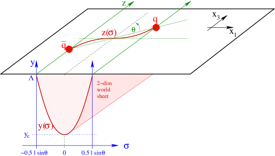
Figure 3: Schematic picture of a $q\bar{q}$-dipole, moving along the $x_{3}$-direction. The dipole is oriented along an arbitrary orientation $\theta$ in the $(x_{1},x_{3})$-plane. The trajectories, along which the quark and antiquark propagate, specify the boundary ${\cal C}$ of a two-dimensional world sheet, which extends into the 5-th bulk dimension $y=r/r_{0}$. The shape of this world sheet is characterized by the functions $y(\sigma)$ and $z(\sigma)$, where $\sigma=x_{1}$. By symmetry, $y$ has a turning point at $y(\sigma=0)=y_{c}$. For generic values of the angle $\theta$, the solution $z(\sigma)$ deviates from a straight line.

In section 3.1, we analyzed the quark-antiquark potential for a $q\bar{q}$-dipole which was oriented in the $x_{1}$ direction and which propagated orthogonal to its orientation along the $x_{3}$ direction with velocity $v=\tanh\eta$. Here, we extend this analysis to the case where the dipole is tilted by an arbitrary angle $\theta$ with respect to its direction of motion, see Fig. 3. For $\theta=\pi/2$, we recover the results obtained in section 3.1 above.

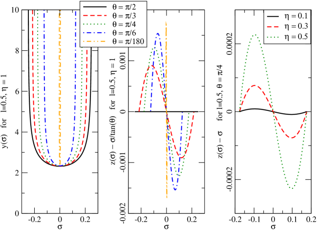
Figure 4: Solutions $y(\sigma)$, $z(\sigma)$ of the differential equations (86) and (87) with boundary conditions (82) for different orientation angles $\theta$ and rapidity $\eta$. These solutions characterize the two-dimensional world sheet bounded by the Wilson loop. For definitions, see Fig. 3 and text. Left panel: $y(\sigma)$ for $\eta=1$ for varying $\theta$. Middle panel: $z(\sigma)-\sigma/\tan\theta$ for $\eta=1$ for varying $\theta$. As Fig. 3 illustrates, $z(\sigma)-\sigma/\tan\theta$ would be zero if the projection of the string onto the D3-brane at $y=\Lambda$ were a straight line. Third panel: $z(\sigma)-\sigma/\tan\theta$ for $\theta=\pi/4$ for varying $\eta$.

We work in the boosted metric (31), in which the dipole is at rest. The dipole lies in the $(x_{1},x_{3})$-plane and the parametrization of the two-dimensional world sheet of the corresponding Wilson loop is

$$\tau=t\,,\qquad\sigma=x_{1}\,,\qquad x_{2}={\rm const.}\,,\qquad x_{3}=x_{3}(\sigma)\,,\qquad r=r(\sigma)\,.$$ (80)

For a dipole with length $L$ whose orientation makes an angle $\theta$ with its direction of propagation (the $x_{3}$-direction) the projections of the dipole on the $x_{1}$ and $x_{3}$ axis are of length $L\sin\theta$ and $L\cos\theta$, respectively. We define dimensionless coordinates

$$y=\frac{r}{r_{0}}\,,\qquad z=x_{3}\frac{r_{0}}{R^{2}}\,,\qquad\tilde{\sigma}=\sigma\frac{r_{0}}{R^{2}}\,,\qquad l=L\frac{r_{0}}{R^{2}}\,,$$ (81)

and drop the tilde. The boundary conditions on $y(\sigma)$ and $z(\sigma)$ then become

$$y\left(\pm\frac{l}{2}\sin\theta\right)=\Lambda\,,\qquad z\left(\pm\frac{l}{2}\sin\theta\right)=\pm\frac{l}{2}\cos\theta\,.$$ (82)

Following the calculation of section 3.1, the Nambu-Goto action for (80) can be written in the form (38), namely $S({\cal C})=\sqrt{\lambda}{\cal T}T\int_{0}^{l/2}d\sigma{\cal L}$, with the Lagrangian reading

$${\cal L}=\sqrt{\left(y^{4}-{\cosh^{2}\eta}\right)\left(1+{y^{\prime 2}\over y^{4}-1}\right)+z^{\prime 2}\left(y^{4}-1\right)}\,,$$ (83)

where $y^{\prime}$ and $z^{\prime}$ denote derivatives with respect to $\sigma$. The Hamiltonian is

$${\cal H}={\cal L}-y^{\prime}\frac{\partial{\cal L}}{\partial y^{\prime}}-z^{\prime}\frac{\partial{\cal L}}{\partial z^{\prime}}={y^{4}-\cosh^{2}\eta\over{\cal L}}=q\,,$$ (84)

a constant of the motion. The momentum conjugate to $z$

$$\frac{\partial{\cal L}}{\partial z^{\prime}}=\frac{y^{4}-1}{\cal L}z^{\prime}=p\,$$ (85)

is also a constant of the motion. For a time-like world sheet, the constants of motion $q$ and $p$ must be real. The equations of motion can be written in the form

$$q^{2}y^{\prime 2} = (y^{4}-\cosh^{2}\eta)(y^{4}-1-p^{2})-q^{2}(y^{4}-1)\,,$$ (86)

$$q^{2}z^{\prime 2} = p^{2}\left(\frac{y^{4}-\cosh^{2}\eta}{y^{4}-1}\right)^{2}\,.$$ (87)

Generic features of their solutions have been pointed out in Ref. [31] already. Fig. 4 shows numerical results. Since $y^{\prime}$ depends only on $y$ and since the boundary condition (82) for $y$ is symmetric under $\sigma\to-\sigma$, $y(\sigma)$ must be an even function of $\sigma$. It descends ($y^{\prime}<0$) for $-l/2\sin\theta<\sigma<0$ and then ascends for $0<\sigma<l/2\sin\theta$. These features are clearly seen in Fig. 4. The turning point $y_{c}=y(0)$ satisfies the condition

$$\left(y_{c}^{4}-\cosh^{2}\eta\right)\left(y_{c}^{4}-1-p^{2}\right)-q^{2}\left(y_{c}^{4}-1\right)\equiv 0\,.$$ (88)

Connecting the $q\bar{q}$-pair by a straight line in the $(x_{1},x_{3})$-plane would correspond to $z(\sigma)=\sigma/\tan\theta$. To test for deviations of the string world sheet away from this straight line, we plot $z(\sigma)-\sigma/\tan\theta$ in Fig. 4. We find a deviation of sinusoidal form for all angles except $\theta=0,\pi/2$. As an aside, we note that if one thinks of the two-dimensional world sheet as a flat piece of paper, draws on it a straight line connecting $q$ and $\bar{q}$, and rolls it up as depicted in Fig. 3, then the projection of this straight line on the $(x_{1},x_{3})$-plane would show a qualitatively similar sinusoidal wiggle. However, the use of this analogy is limited, since we cannot specify in which sense or to what extent the two-dimensional world sheet is flat. Also, the observed deviation from the straight line behavior $z(\sigma)=\sigma/\tan\theta$ depends on rapidity. For $\eta=0$, no deviation is possible since no direction in the $(x_{1},x_{3})$-plane is singled out. For increasing values of $\eta$, the deviation increases as seen in Fig. 4.

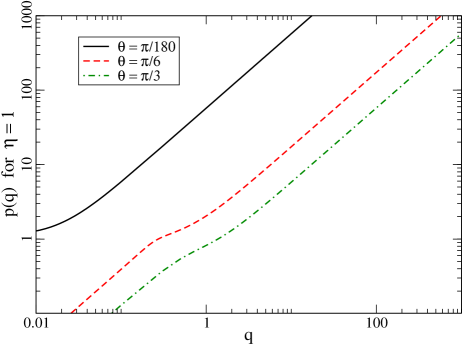
Figure 5: The integration constant $p$ as a function of the integration constant $q$ for $\eta=1$ and several fixed values of the orientation angle $\theta$. This relation is defined by eqs. (89) and (90). Along one of these curves, $\ell$ changes with $q$ as shown in Fig. 6.

The constants $q$ and $p$ must be related to the values of $l$ and $\theta$. The relationships are obtained by integrating the equations of motion (86) and (87), giving

$$\frac{l}{2}\sin\theta=q\int_{y_{c}}^{\infty}\frac{dy}{\sqrt{\left(y^{4}-\cosh^{2}\eta\right)\left(y^{4}-1-p^{2}\right)-q^{2}\left(y^{4}-1\right)}}\,,$$ (89)

$$\frac{l}{2}\cos\theta=p\int_{y_{c}}^{\infty}\frac{y^{4}-\cosh^{2}\eta}{y^{4}-1}\frac{dy}{\sqrt{\left(y^{4}-\cosh^{2}\eta\right)\left(y^{4}-1-p^{2}\right)-q^{2}\left(y^{4}-1\right)}}\,.$$ (90)

With $q$ and $p$ determined, the $q\bar{q}$ static potential in a moving thermal background then reads

$$E(l,\theta;\eta) = S({\cal C})-S_{0}$$ (91)

$$= \sqrt{\lambda}{\cal T}T\int_{y_{c}}^{\infty}\left[\frac{(y^{4}-\cosh^{2}\eta)}{\sqrt{\left(y^{4}-\cosh^{2}\eta\right)\left(y^{4}-1-p^{2}\right)-q^{2}\left(y^{4}-1\right)}}-1\right]\,dy$$

$$-\sqrt{\lambda}{\cal T}T\left(y_{c}-1\right)\,.$$

Here, the subtraction term $S_{0}$, given in (46) is the action for two isolated strings described by the dragging solution of Refs. [23, 24] and Appendix A.

We have evaluated the potential $E(l,\theta;\eta)$ as a function of the size $l$ of the dipole, its orientation $\theta$ with respect to its direction of motion, and its velocity $v=\tanh\eta$ with respect to the thermal heat bath. Since the potential in (91) is written in terms of the integration constants $q$ and $p$, it is useful to determine first how $p$ depends on $q$ for fixed $\theta$ and $\eta$. To do this, we write $\tan\theta$ as the ratio of Eqs. (89) and (90). We find $p(q)$ to be a monotonously increasing function, whose slope decreases with increasing angle $\theta$, see Fig. 5. For the maximal angle $\theta=\pi/2$, $p$ vanishes independent of the value of $q$. This is the case of a dipole oriented orthogonal to the wind, where Eq. (89) reduces to Eq. (43), and the present calculation becomes that of Section 3.1. For the opposite limit of a dipole oriented parallel to the wind, $\theta=0$, the parametrization (80), (82) of the two-dimensional world sheet does not apply. However, the Nambu-Goto action is reparametrization invariant and, as described in Appendix B, in a parametrization which is suitable for $0\leq\theta<\pi/2$ we find that the measurable quantity $E(l,\theta,\eta)$ depends smoothly on $\theta$ for $\theta\to 0$.

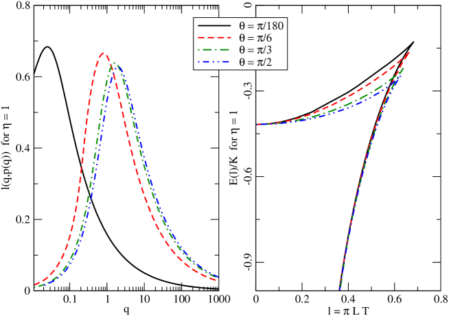
Figure 6: Left panel: The size $l$ of the dipole and its orientation angle $\theta$ define the integration constants $q$ and $p$, see eqs. (89) and (90). The plot shows $l$ as a function of $q$ for several fixed angles $\theta$. Along each of these curves $p$ varies as shown in Fig. 5. Right panel: The static $q\,\bar{q}$-potential (91) for rapidity $\eta=1$ and different orientation angles $\theta$ of the dipole with respect to the direction of motion.

Knowing $p(q)$ for fixed $\eta$ and $\theta$, the rescaled dipole size $l(q)=l(q,p(q))$ can be written as a function of $q$ only. It takes values in the range $l\in\left[0,l_{\rm max}\right]$. Here, the maximal dipole size $l_{\rm max}$ is the screening length above which bound states do not exist. The value of $q$ at which the maximum of $l(q)$ occurs depends strongly on the angle $\theta$, as shown in the left panel of Fig. 6. This is a feature of our parametrization: for smaller angle $\theta$, $p(q)$ is a more steeply rising function (see Fig. 5), and most of the $\theta$-dependence of $l(q,p(q))$ comes from the $p(q)$-dependence. The value of $l_{\rm max}$ decreases slightly with increasing angle $\theta$. This is consistent with the expectation that the dipole is easier to dissociate if it is oriented orthogonal to the direction of the wind, but the effect is slight.

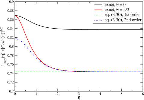
Figure 7: The screening length $l_{\rm max}$ times its leading large-$\eta$ dependence $\sqrt{\cosh(\eta)}$. The exact results are given for dipoles oriented perpendicular to the wind ($\theta=\pi/2$) and parallel to the wind ($\theta=0$). The $\theta=\pi/2$ curve is compared to the analytical large-$\eta$ approximation (48). Keeping only the first term in this analytical expression corresponds to a horizontal line on the figure; including the term proportional to $(\cosh\eta)^{-5/2}$ improves the agreement with the exact result.

With $p(q)$ determined, the $q\bar{q}$-static potential $E(l(q,p(q)),\theta,\eta)$ also becomes a function of $q$ only. This defines curves $\{l(q),E(l(q))\}$, parametrized by the integration constant $q\in\left[0,\infty\right]$. The $q\bar{q}$ static potential (91) is a double-valued function of $l$ in the range $l\in\left[0,l_{\rm max}\right]$, see the right panel of Fig. 6. The configurations whose energy is given by the upper branch of $E(l)$ are presumably unstable, as has been shown explicitly for $\theta=\pi/2$ in Ref. [36]. The lower branch displays the typical short-distance behavior of a $q\bar{q}$ binding potential. For fixed rapidity $\eta$, this potential shows the expected $\theta$-dependence: the $q\bar{q}$ pair is more strongly bound if the dipole is aligned with the direction of motion, and this binding decreases as the dipole presents itself at a larger angle with respect to the wind, see Fig. 5.

In Fig. 2 in Section 3, we have explored the $\eta$-dependence of the $q\bar{q}$ static potential for a dipole oriented orthogonal to the wind. The screening length displays the dominant Lorentz-$\gamma$ dependence $l_{\rm max}\propto 1/\sqrt{\cosh\eta}=1/\sqrt{\gamma}$, as given in (48). This velocity dependence is much stronger than the angular dependence displayed in Fig. 6. The velocity dependence of the potential $E(l)$, shown on the right hand side of Fig. 2, also shows clearly that the short distance behavior of the potential is not affected by velocity-dependent medium effects. This is a consequence of choosing the regularization prescription (46).

Finally, we show in Fig. 7 the screening length $l_{\rm max}$ multiplied by $\sqrt{\cosh\eta}$. We include curves for $\theta=0$ and $\theta=\pi/2$; those for other angles lie in between these two. Note that both curves have the same value of $l_{\rm max}$ in the $\eta\rightarrow 0$ limit as they must. The flat behavior of these curves at large $\eta$ illustrates that $l_{\rm max}\propto 1/\sqrt{\cosh\eta}$ is the leading large-$\eta$ dependence for all dipole orientations. This leading behavior provides a numerically very accurate approximation ($<1\%$ deviation) for $\eta>2$, and even for $\eta=0$, it is accurate to within 20% (note the suppressed zero in Fig. 7). Including the $(\cosh\eta)^{-5/2}$ term in the analytical expansion (48) improves the description.

6 Discussions and Conclusions

In Section 2, we reviewed the physical arguments why the expectation value of the time-like Wilson loop which describes the quark-antiquark potential must be the exponential of an imaginary quantity whereas the expectation value of the light-like Wilson loop which arises in the physics of deep inelastic scattering, proton-nucleus collisions, and the calculation of the jet quenching parameter relevant to parton energy loss in heavy ion collisions is instead the exponential of a real quantity. In Section 3, we saw how these results emerge by direct calculation in ${\cal N}=4$ SYM theory at strong coupling, where via the AdS/CFT correspondence the calculation of the expectation values of these two types of Wilson loops reduces to the evaluation of the action of an extremal string world sheet, time-like in the first case and space-like in the second. These aspects of our paper are discussed at length in Section 3 and we shall not discuss them further here.

This section incorporates several different discussions, while along the way summarizing many of our conclusions. In Section 6.1, we summarize what we have learned from our calculations of screening in a hot wind. We compare our calculation of the jet quenching parameter $\hat{q}$ to the very different approach to energy loss in Refs. [23, 24, 25, 26, 27] in Section 6.2. In Section 6.3, we compare our calculation of $\hat{q}$ in ${\cal N}=4$ SYM to that extracted from RHIC data. Given that we find surprisingly good agreement between $\hat{q}_{SYM}$ and that extracted from RHIC data, in Section 6.4 we enumerate the differences and similarities between ${\cal N}=4$ SYM and QCD. Finally, in Section 6.5 we collect what is known about how $\hat{q}$ changes from the quark-gluon plasma of one gauge theory to that of another, including deriving a new result which allows the determination of $\hat{q}$ in any conformal theory with a gravity dual. We use this result to estimate $\hat{q}_{QCD}/\hat{q}_{SYM}$.

6.1 Velocity dependence of screening length

We can summarize what we have learned from our calculation in Sections 3 and 5 of the quark-antiquark potential and screening length in a hot wind as follows. We find that the screening length $L_{\rm max}$ of an external quark in an ${\cal N}=4$ SYM plasma with velocity $v=\tanh\eta$ can be written as

$$L_{\rm max}={f(\eta,\theta)\over\pi T\sqrt{\cosh\eta}}\ ,$$ (92)

where ${\theta}$ is the angle between the orientation of the dipole and the velocity of the moving thermal medium in the rest frame of the dipole. $f(\eta,{\theta})$ is only weakly dependent on both of its arguments. That is, it is close to constant. In fact, for any values of $\eta$ and $\theta$, $f(\eta,\theta)$ lies between 0.74 and 0.87. The limiting cases are $f(\eta=0)\simeq 0.87$ for all $\theta$, and $f(\infty,{\pi\over 2})\simeq 0.74$. For a given $\eta$, $f(\eta,{\theta})$ is a monotonically decreasing function of ${\theta}$ as ${\theta}$ varies from $0$ to $\pi/2$. For a given ${\theta}$, $f(\eta,\theta)$ is a monotonically decreasing function of $\eta$. As $\eta\to\infty$, we find $f(\eta,{\theta})=f(\infty,{\theta})(1+{\cal O}(1/\cosh^{2}\eta))$.

For ${\cal N}=4$ SYM theory, since the energy density $\varepsilon\propto T^{4}$, in the large $\eta$ limit equation (92) can also be thought of as

$$L_{\rm max}\propto{1\over\varepsilon(\eta)^{1\over 4}}\ ,$$ (93)

where $\varepsilon(\eta)=\cosh^{2}\eta\,\varepsilon(0)$ is the energy density of the boosted medium.

As discussed in Ref. [31], if the velocity scaling of $L_{\rm max}$ that we have found, namely (92) and (93), holds for QCD, it will have qualitative consequences for quarkonium suppression in heavy ion collisions at RHIC and LHC. Since our discussion in earlier sections only involves the AdS₅ part of the geometry, the scaling (93) applies to any conformal field theory with a gravity dual at finite temperature. To the extent that the QGP of QCD at RHIC temperature is close to being conformal, one is tempted to view this as a support of the applicability of (92) and (93) to QCD. The results of Ref. [30] further support this view. These authors studied large-spin mesons in a hot wind in a confining, nonsupersymmetric theory and found that they dissociate beyond a maximum wind velocity. The relation between the size $L$ of these mesons and their dissociation velocity $v$ is consistent with $L\propto(1-v^{2})^{1/4}$.

For more general theories with a gravity dual, one can use the generic metric (118) which we introduce below to study the screening length. A nice argument presented by Caceres, Natsuume and Okamura in Ref. [33] indicates that in the large $\eta$ limit, one would generically have

$$L_{\rm max}\propto{1\over\varepsilon(\eta)^{\nu}}$$ (94)

for some index $\nu$. In particular, for any gauge theory which is dual to an asymptotically AdS₅ geometry, one would find $\nu={1\over 4}$ as in (93). Examples include ${\cal N}=4$ SYM with nonzero $R$-charge chemical potentials, studied in Refs. [33, 35]. (Note that since chemical potentials introduce additional mass scales, the dependence of $L_{\rm max}$ on temperature is rather complicated and it is (93) which generalizes, not (92).)

For non-conformal theories the scaling index $\nu$ can deviate from $1/4$. One measure of the deviation from conformality is the deviation of the sound velocity from the conformal value of $1/\sqrt{3}$. Following a similar argument in Ref. [16] concerning the value of $\hat{q}$ in non-conformal theories, Caceres, Natsuume and Okamura suggested that for theories which are close to being conformal, the index $\nu$ may profitably be written as

$$\nu={1\over 4}+c\delta+\cdots,\qquad\delta={1\over 3}-v_{s}^{2}$$ (95)

with $c$ some constant. For the cascading gauge theories of Ref. [88], $c=-9/16$ meaning that if $v_{s}^{2}\simeq 0.27-0.31$ in these theories as is the case in QCD at $T\sim 1.5T_{c}$ [89], the index is $\nu\simeq 0.21-0.24$. This suggests that for QCD the scaling (93) with $\nu=1/4$ should be a very good guide.

As discussed at the end of Section 3.1, the velocity scaling (93) describes how screening lengths and, correspondingly, dissociation temperatures drop for quarkonia moving through the thermal medium with some relative velocity, and so should be included in the modelling of quarkonium suppression. The $p_{T}$-dependent pattern of quarkonium suppression predicted by (93) will be tested in future heavy ion experiments at RHIC and the LHC.

6.2 Comparison with energy loss via drag

Before comparing our result for $\hat{q}$ with that extracted from RHIC data, which we shall do in Section 6.3, we discuss the differences between our approach and recent calculations [23, 24, 25, 26, 27] of how an external quark loses energy while being dragged through an ${\cal N}=4$ SYM plasma. In Appendix A (see (141)) we have reproduced the “dragging string solution” of Refs. [23, 24] for a string attached to and trailing behind an isolated moving test quark, since we need it as the subtraction term in our calculation of the quark-antiquark potential in Section 3.1.

To describe the results of Refs. [23, 24, 25] in their proper context, let us start with the relativistic generalization of the Langevin equations for a quark moving through some thermal medium (see for example Ref. [99, 25])

$${dp_{L}\over dt} = -\mu(p_{L})p_{L}+\xi_{L}(t)\ ,$$ (96)

$${dp_{T}\over dt} = \xi_{T}(t)\ ,$$ (97)

where $p_{L}$ and $p_{T}$ are the longitudinal and transverse momentum of the quark, respectively. (We have simplified the notation by dropping the spatial indices on transverse quantities.) Henceforth we shall denote $p_{L}$ by $p$. $\xi_{L}$ and $\xi_{T}$ are random fluctuating forces in the longitudinal and transverse directions, which satisfy

$$\langle\xi_{L}(t)\xi_{L}(t^{\prime})\rangle = \kappa_{L}(p)\delta(t-t^{\prime})\ ,$$ (98)

$$\langle\xi_{T}(t)\xi_{T}(t^{\prime})\rangle = \kappa_{T}(p)\delta(t-t^{\prime})\ .$$ (99)

$\kappa_{L}(p)$ and two times $\kappa_{T}(p)$ describe how much longitudinal and transverse momentum squared is transferred to the quark per unit time. Note that at zero velocity, $\kappa_{L}(0)=\kappa_{T}(0)$ whereas for $p>0$ one expects that $\kappa_{L}(p)\neq\kappa_{T}(p)$. Also, upon assuming that the momentum fluctuations of the particle are in equilibrium with the thermal medium, as appropriate at zero velocity, a fluctuation-dissipation theorem relates $\mu(0)$ to $\kappa_{L}(0)$ via the Einstein relation

$$\mu(0)=\frac{\kappa_{L}(0)}{2mT}\ ,$$ (100)

where $m$ is the static mass of the quark. The relation (100) is also not expected to hold for $p>0$. (See Ref. [99] for examples.)

The central result of Refs. [23, 24] is that an isolated quark moving through the ${\cal N}=4$ SYM plasma with its trailing, dragging, string feels a drag force proportional to $p$, described by a momentum independent drag coefficient

$$\mu(p)={\pi\sqrt{\lambda}\over 2m}T^{2}\ .$$ (101)

Independently, $\kappa_{L}(0)$ in the ${\cal N}=4$ SYM plasma was calculated directly in Ref. [25]. These authors found that $\kappa_{L}(0)$ and $\mu(0)$ in (101) indeed satisfy (100), which can be considered a new consistency check of the AdS/CFT framework.

Eq. (101) demonstrates that in the high energy limit the energy loss mechanism in strongly coupled ${\cal N}=4$ SYM theory is very different from that in QCD. The origin of the difference is the fact that ${\cal N}=4$ SYM is not asymptotically free. In QCD, as discussed in Section 2, the average energy loss of a parton in the high energy limit is independent of $p$ (or at most logarithmically dependent on $p$) and it is proportional to the square of the distance travelled through the medium. There, the dominant mechanism by which a high energy parton loses its energy is through radiating gluons which have a high enough transverse momentum $k_{T}$ (and an even higher energy) that $\alpha_{s}$ evaluated at $k_{T}$ is weak, meaning that the dominant energy loss processes can be described perturbatively, with nonperturbative physics at scales of order the temperature coming in only via the description of the repeated soft interactions between the radiated gluon and the medium, and between the original high energy parton and the medium. The effect of these nonperturbative soft interactions is encoded in the jet quenching parameter $\hat{q}$, which can be defined nonperturbatively via a light-like Wilson loop as described in Section 2.

In Ref. [15] and in the present paper, we seek insights about $\hat{q}$ in QCD by calculating the analogous quantity in ${\cal N}=4$ SYM. We do not attempt to describe the full process of energy loss in ${\cal N}=4$ SYM because the asymptotic freedom of QCD is crucial to the description of the radiative parton energy loss process which dominates at high energies, making it impossible to model the physics of QCD parton energy loss at high energies in a theory like ${\cal N}=4$ SYM which is strongly interacting at all scales.

Even though the drag coefficient (101) describes energy loss in a ${\cal N}=4$ SYM plasma even for quarks moving relativistically [23], it cannot be used to extract $\hat{q}$ or $\kappa_{T}(p\to\infty)$. As we remarked after equation (99), except in the low-velocity limit one does not expect $\kappa_{T}(p)$ to be equal to $\kappa_{L}(p)$ or $\kappa_{L}(p)$ to be related to $\mu(p)$ via the Einstein relation. Indeed, the direct calculation of $\kappa_{L}$ in Ref. [25] manifestly requires modification at nonzero $p$ [100]. The $\kappa_{L}(0)$ found in Ref. [25] and indirectly in Ref. [23] has the same parametric dependence on $\lambda$ and $T$ as $\hat{q}$ in (102), and is smaller than $\hat{q}$ by a purely numerical factor of $\sim 1.20$. This is curious, since the quantity $\kappa_{L}(0)=\kappa_{T}(0)$ has no evident relation to jet quenching (since jets by definition are relativistic) or to the jet quenching parameter $\hat{q}$.

To look for connections between ${\cal N}=4$ SYM energy loss described by (101) and data from RHIC one should then seek circumstances in which all aspects of the energy loss process are strongly coupled. Perhaps the energy loss of quarks which are slowly moving and yet energetic — i.e. quarks which are heavy — is the best example, as stressed by many of the recent papers [23, 24, 25, 26, 27], although extracting the contribution from energy loss to the medium modification of charmed meson production in the regime in which the parent $c$-quark is slowly moving presents considerable challenges. Furthermore, precisely because the entire energy loss process is treated in this approach, further questions like how the ${\cal N}=4$ SYM medium responds to the dragging quark (i.e. “where does the lost energy go?”) can be addressed [27].

6.3 Comparison of $\hat{q}$ of ${\cal N}=4$ SYM with experimental estimate

We turn now to the comparison between $\hat{q}$ in ${\cal N}=4$ SYM with that extracted from current RHIC data. In Eq. (63) we found that

$$\hat{q}_{SYM}=\frac{\pi^{3/2}\Gamma\left(\frac{3}{4}\right)}{\Gamma\left(\frac{5}{4}\right)}\sqrt{\lambda}\,T^{3}\approx 26.69\sqrt{\alpha_{\rm SYM}N_{c}}\,T^{3}\,.$$ (102)

Taking $N=3$ and $\alpha_{\rm SYM}=\frac{1}{2}$, thinking $\alpha_{\rm QCD}=\frac{1}{2}$ reasonable for temperatures not far above the QCD phase transition, we shall use $\lambda=6\pi$ to make estimates. From (102), we find

$$\hat{q}_{\rm SYM} =4.5,10.6,20.7\;{\rm GeV}^{2}/{\rm fm}\qquad{\rm for}\qquad T=300,400,500\,{\rm MeV}\,.$$ (103)

We have computed (102) in the large $N$ and large ’t Hooft coupling $\lambda$ limit and thus it is only the leading order term in a double expansion in $1/\sqrt{\lambda}$ and $1/N^{2}$. There are two sources of contributions to $1/\sqrt{\lambda}$ corrections: from the fluctuation of the string world sheet (23) and from the modification of the background geometry (26) due to ${\alpha^{\prime}}$ corrections. The authors of Ref. [21] find that the leading contribution of the second type of correction is given by

$$\hat{q}_{SYM}(\lambda)=\hat{q}_{SYM}\left(1-1.765\lambda^{-{3\over 2}}+\cdots\right)\ .$$ (104)

If one uses ${\alpha}_{\rm SYM}=\frac{1}{2}$, then the correction from (104) is about $2\%$. The corrections due to fluctuations of the world sheet, the leading order term of which is expected to be of order $1/\sqrt{\lambda}$, are harder to compute and are not known at the moment. $1/N^{2}$ corrections, which require string loop calculations, are also beyond currently available technology. It is worth noting, however, that the ratio of energy density and pressure to their Stefan-Boltzmann values are both quite insensitive to changing $N$ from 3 to 4 to 8 [95].

In a heavy ion collision, $\hat{q}$ decreases with time $\tau$ as the hot fluid expands and cools. The time-averaged $\hat{q}$ which has been determined in comparison with RHIC data is $\overline{\hat{q}}\equiv\frac{4}{(L^{-})^{2}}\int_{\tau_{0}}^{\tau_{0}+L^{-}/\sqrt{2}}\tau\,\hat{q}(\tau)\ d\tau$, found to be around 5-15 GeV${}^{2}/$fm [96, 97]. If we assume a one-dimensional Bjorken expansion with $T(\tau)=T_{0}\left(\frac{\tau_{0}}{\tau}\right)^{1/3}$, take $\tau_{0}=0.5$ fm, and take $L^{-}/\sqrt{2}=2$ fm, the estimated mean distance travelled in the medium by those hard partons which “escape” and are detected [97], we find that to obtain $\overline{\hat{q}}=5$ GeV${}^{2}/$fm from (102) we need $T_{0}$ such that $T(1~{}{\rm fm})\approx 310$ MeV, only slightly higher than that expected from hydrodynamic modelling [98]. With $L^{-}/\sqrt{2}=1.5$ fm, we find $\overline{\hat{q}}=5$ GeV${}^{2}/$fm for $T(1~{}{\rm fm})\approx 280$ MeV, fully consistent with expectations. There are currently too many uncertainties in the various components of this comparison to make a strong statement, but it seems clear that the $\hat{q}$ given by (102) that we have calculated in the quark-gluon plasma of ${\cal N}=4$ SYM is in qualitative agreement with $\overline{\hat{q}}=5$ GeV${}^{2}/$fm, which is in turn consistent with RHIC data.

The value obtained from (102) assumes that the medium is static. However, in a relativistic heavy ion collision, the medium itself develops strong collective flow, meaning that the hard parton is traversing a moving medium — it feels a wind. Thus to compare (102) with the experimental estimate we should include the effects of the wind on $\hat{q}$ that we discussed in Section 4. We found in Eq. 79 that

$$\hat{q}=\gamma_{f}(1-v_{f}\cos{\theta})\,\hat{q}_{0}\ ,$$ (105)

where $v_{f}=\tanh\eta_{f}$ is the velocity of the wind, $\gamma_{f}=1/\sqrt{1-v_{f}^{2}}$, and $\theta$ is the angle between the direction of motion of the hard parton and the direction of the wind. $\hat{q}_{0}$ is the value of $\hat{q}$ in the absence of a wind. The result (105) for the dependence of $\hat{q}$ on collective flow is valid in QCD and in ${\cal N}=4$ SYM and in the quark-gluon plasma of any other gauge theory, since its derivation (see Section 4) relies only on properties of Lorentz transformations. If we crudely guess that head winds are as likely as tail winds, and that the typical transverse wind velocity seen by a high energy parton is about half the speed of light, $\hat{q}$ is increased relative to that in (102) by a factor of 1.16. A credible evaluation of the consequences of (105) for the time-averaged $\hat{q}$ extracted from data will, however, require careful modelling of the geometry of the collision and the time-development of the collective flow velocity, as in Refs. [85, 86, 87].

The weak-coupling QCD estimate of $\hat{q}$ given in (18) is, when evaluated with $\alpha_{s}=1/2$, smaller than that in (103) by about a factor of 5. This means that in order to make the weak-coupling estimate consistent with data from RHIC, we would have to choose $\alpha_{s}>1$, certainly beyond weak-coupling. The strong coupling calculation of $\hat{q}$ in ${\cal N}=4$ SYM is certainly in better agreement with data from RHIC than the weak-coupling calculation in QCD. The obvious question, then, is how much the strong coupling result will change as one modifies the theory from ${\cal N}=4$ SYM towards, and ultimately to, QCD. We shall describe the current state of our ability to answer this question in Section 6.5.

The BDMPS description of radiative parton energy loss, with the nonperturbative physics of the medium entering through the jet quenching parameter $\hat{q}$, is appropriate in the high parton energy limit. It is only by comparison to data that we can learn whether the jets being quenched at RHIC are sufficiently energetic for their energy loss to be described well by this formalism. To date this comparison has been broadly successful, albeit with $\hat{q}$ seen as a free parameter. If we understood the QCD prediction for $\hat{q}$ as a function of temperature in a strongly interacting quark-gluon plasma even at the factor of two level, this would make this comparison more stringent. And, it would turn $\hat{q}$ into a “thermometer” with a calibration error of only a factor of $2^{1/3}$, which would be an exceptionally valuable addition since one of the biggest current weaknesses in our understanding of RHIC phenomena is that we do not have an experimental measure of the temperature at, say, a time of 1 fm after the collision. In the next two subsections, we first frame the questions that need to be thought through if it is to be possible to go from our calculation of $\hat{q}$ in ${\cal N}=4$ SYM to a factor of two understanding of $\hat{q}$ in QCD, and then review and extend the calculations of $\hat{q}$ in various other gauge theories, yielding a conjecture for how to estimate $\hat{q}$ in QCD at a semi-quantitative level, still with many caveats. Our conjecture is that ${\hat{q}}_{QCD}/{\hat{q}}_{SYM}$ is of the order of $\sqrt{47.5/120}\simeq 0.63$, namely the square root of the ratio of the numbers of degrees of freedom in the two theories.

6.4 ${\cal N}=4$ SYM versus QCD

We found in Section 6.3 that $\hat{q}$ calculated in ${\cal N}=4$ SYM theory is close to the value extracted from RHIC data. Given that RHIC is probing the quark-gluon plasma of QCD, is this agreement meaningful or accidental? In what respects can the strongly interacting plasma of ${\cal N}=4$ SYM theory give a reasonable description of the quark-gluon plasma in QCD? After all, at a microscopic level ${\cal N}=4$ SYM is very different from QCD:

• The theory is conformal, supersymmetric and contains additional global symmetry. The coupling does not run and there is no confinement.

• No dynamic quarks, no chiral symmetry and no chiral symmetry breaking.

• Additional scalar and fermionic fields in the adjoint representation.

These features of course make the vacuum sectors of the two theories very different. However, if the quark-gluon plasma in QCD is strongly interacting, as indicated by data from RHIC, then one may ask whether the macroscopic properties, both thermodynamic and dynamic, of quark-gluon plasma at sufficiently strong coupling may be insensitive to differences between the theories which seem stark in vacuum. It is often the case that macroscopic properties of a sufficiently excited many-body system are not sensitive to the detailed underlying dynamics, with systems within the same universality class exhibiting similar phenomena. We are used to the idea that all metals, or all liquids, or all ferromagnets have common, defining, characteristics even though they may differ very significantly at a microscopic level. What we are asking here is what are the defining commonalities of quark-gluon plasmas in different theories, and in what instances do these commonalities allow qualitative or semi-quantitative lessons learned about the quark-gluon plasma of one theory to be applied to that of another.

Returning to the differences between QCD and ${\cal N}=4$ SYM, many are obviously irrelevant to a comparison between strongly-coupled plasmas in the two theories. After all, supersymmetry is explicitly and badly broken at high temperature and, above $T_{c}$ in QCD, there is no confinement and no chiral condensate. Furthermore, in a strongly interacting liquid there are, by definition, no well-defined, long-lived quasiparticles anyway, making it plausible that observables or ratios of observables can be found which are insensitive to the differences between microscopic degrees of freedom and interactions. Because ${\cal N}=4$ SYM is a conformal theory whereas QCD is not, ${\cal N}=4$ SYM cannot be used to describe QCD at or below its phase transition at $T\sim T_{c}$, and cannot be used to describe QCD at asymptotically high temperatures. However, there are a variety of indications from lattice QCD calculations (enumerated below) that QCD thermodynamics is reasonably well approximated as conformal in a range of temperatures from about $2T_{c}$ up to some higher temperature not currently determined. It is not currently known whether the quark-gluon plasma of QCD, as explored at RHIC and in lattice QCD calculations, and that of ${\cal N}=4$ SYM, as explored using AdS/CFT calculations, are in the same universality class, or even in what sense this question could be made precise. However, given the rapidly increasing list of similarities between the two quark-gluon plasmas, it does not seem too far-fetched to imagine. Here is a list of some of the similarities between the quark-gluon plasmas of the two theories, notwithstanding the stark differences between their vacua, with thermodynamic comparisons listed first followed by dynamic comparisons:

• Above about $1.2T_{c}$, the ratio of the energy density $\varepsilon$ in 2- and 3-flavor QCD to that in the absence of interactions is close to $T$-independent and takes on the value of about 0.8 [101, 92, 89]. In zero-flavor QCD, this ratio is closer to 0.9 [102]. In ${\cal N}=4$ SYM, this ratio is $3/4$ in the $\lambda\rightarrow\infty$ limit [93] and is 0.8 for $\lambda\sim 11$ [94].

• Above about $2.5T_{c}$, the ratio of the pressure $P$ in 2- or 3-flavor QCD to that in the absence of interactions is also about 0.8. In zero-flavor QCD, this ratio is closer to 0.9 [102]. In ${\cal N}=4$ SYM, this ratio must be the same as that defined via the energy density, a condition that is satisfied well in QCD. Note, however, that for $T\lesssim 2.5T_{c}$, the deviation from conformality parametrized by $\varepsilon-3P$ is significant. This suggests that the use of a conformal theory like ${\cal N}=4$ SYM as a model for the quark-gluon plasma may be more quantitatively reliable for heavy ion collisions at the LHC than at RHIC, since RHIC is likely exploring temperatures that are less than $2T_{c}$ whereas the LHC can be expected to reach temperatures that are higher by about a factor of two.

• All the results in ${\cal N}=4$ SYM have been obtained in the $N\rightarrow\infty$ limit. Although corrections are expected to be of order $1/N^{2}$, they have not been computed. It is therefore very useful to test how the quantities on the QCD side of these comparisons change with $N$. One example of such a test is the calculation of Ref. [95], which finds that the ratio of the pressure to its noninteracting value changes very little as $N$ is changed from 3 to 4 to 8.

• The square of the speed of sound in the QCD quark gluon plasma is close to $1/3$, the value for a conformal theory, for $T\gtrsim 2T_{c}$; at $T=1.5T_{c}$, it is already $\simeq 0.27-0.31$ [102, 103, 104, 105, 89].

• The screening length defined by the potential between a quark and antiquark at rest is $0.869/\pi T\simeq 0.28/T$ in ${\cal N}=4$ SYM in the large $N$ and $\lambda$ limits, as calculated in Section 3 and as calculated first in Refs. [28]. In QCD the screening length is not sharply defined, since the potential does not change suddenly to zero, but operational definitions exist in the literature. For QCD with zero [106] and two [107] flavors, it is $\sim 0.7/T$ and $\sim 0.5/T$, respectively. QCD and ${\cal N}=4$ SYM are therefore qualitatively comparable in this regard, with the quantitative difference between them plausibly reflecting the larger number of degrees of freedom in ${\cal N}=4$ SYM.

• Turning now to dynamic quantities, the shear viscosity in units of the entropy density is $1/4\pi$ in ${\cal N}=4$ SYM in the $\lambda\rightarrow\infty$ limit [3], and is $\simeq 1.25/4\pi$ for $\lambda=6\pi$ [7]. Given the degree to which data on the azimuthal anisotropy of RHIC collisions are well-described by zero-viscosity hydrodynamics, the ratio of the shear viscosity to the entropy density has been estimated to be comparably small in the quark-gluon plasma at RHIC [11]. A quantitative extraction of $\eta$ from RHIC data requires viscous hydrodynamic calculations, which are currently being pursued by various groups [108].

• In ${\cal N}=4$ SYM, the quark-antiquark screening length scales with velocity according to $L_{s}(v)\sim L_{s}(0)/\sqrt{\gamma}$, as discussed in Ref. [31] and Sections 3.1 and 5 above. Comparison of this predicted scaling to QCD awaits data from RHIC on the $p_{T}$-dependence of $J/\Psi$ suppression at RHIC at $p_{T}>5$ GeV and on the pattern of $p_{T}$-dependence of $J/\Psi$ and Upsilon suppression at the LHC.

• As we have discussed in Section 6.3, the jet quenching parameter $\hat{q}$ in ${\cal N}=4$ SYM is close to the value extracted from RHIC data [15].

To understand whether the above similarities are meaningful, one avenue is to study strongly interacting quark-gluon plasmas in other non-Abelian gauge theories with dual gravity descriptions and see whether a general picture emerges. In the case of the ratio of the shear viscosity to the entropy density, it was indeed found that this ratio is the same in a broad class of gauge theories [4, 5]. A necessary (but not sufficient) condition for this striking lack of dependence on the nature of the microscopic theory is that the dependence on the number of degrees of freedom cancels in the dimensionless ratio. In thinking about how the value of $\hat{q}$, a dimensionful quantity, may change in going from ${\cal N}=4$ SYM to QCD, it seems to us that the two most pressing questions are how $\hat{q}$ depends on the number of degrees of freedom and on the fact that QCD includes fundamentals whereas all the degrees of freedom in ${\cal N}=4$ SYM are adjoints. These seem to have greater potential to change $\hat{q}$ significantly than do $1/\sqrt{\lambda}$ corrections, $1/N^{2}$ corrections or corrections due to the deviation away from conformality. We cannot currently address the effect of fundamentals. In Section 6.5, we consider how $\hat{q}$ depends on the number of degrees of freedom.

6.5 The jet quenching parameter and degrees of freedom

One qualitative feature of Eq. (102) is that at strong coupling $\hat{q}$ is proportional to $\sqrt{\lambda}$, not to the number of degrees of freedom $\sim N^{2}$. This means that at strong coupling, $\hat{q}$ cannot be thought of as “measuring” either the entropy density $s$ or what is sometimes described as a “gluon number density” or $\varepsilon^{3/4}$ as had been expected [76], since both $s$ and the energy density $\varepsilon$ are proportional to $N^{2}\lambda^{0}$. Whereas the ratio of the shear viscosity to $s$ turns out to be universal in theories with gravity duals, the ratio $\hat{q}/s$ vanishes in the large-$N$ limit. Even though (102) upends prior intuition on this point, it nevertheless seems that $\hat{q}$ should have some straightforward dependence on the number of degrees of freedom in the theory. We shall now try to make this intuition precise.

We first examine how $\hat{q}$ of different conformal field theories with a type IIB supergravity dual compare to each other, using that of ${\cal N}=4$ SYM as a reference point. The ten-dimensonal metric dual to a conformal field theory at zero temperature can be written in the form

$$ds^{2}_{10}={\Omega}^{2}(y)R^{2}\left(ds^{2}_{AdS_{5}}+ds^{2}_{M_{5}}(y)\right)\ ,$$ (106)

where $R$ is the curvature radius of AdS₅ and the metric for AdS₅ inside the parenthesis is normalized to have curvature radius unity. $ds^{2}_{M_{5}}$ is the metric of an internal five-dimensional manifold. The warp factor ${\Omega}^{2}(y)$ depends only on the coordinates $y$ of the internal manifold. To put the theory at finite temperature, one replaces $ds^{2}_{AdS_{5}}$ by the metric of (26) of an AdS-Schwarzschild black hole. The computation of $\hat{q}$ is identical to what we have done before and we find that (cf. (63))

$$\hat{q}=\frac{\pi^{3/2}\Gamma\left(\frac{3}{4}\right)}{\Gamma\left(\frac{5}{4}\right)}{{\Omega}^{2}(y)R^{2}\over{\alpha^{\prime}}}\,T^{3}\,.$$ (107)

We shall compare different theories at fixed values of $N$, $\lambda=4\pi g_{s}N$ and $T$. Note that the ${\cal N}=4$ SYM relation $\sqrt{\lambda}=R^{2}/{\alpha^{\prime}}$ is modified in this more general context, as we shall see below in (108).

Let us first consider theories in which the warp factor is trivial, i.e. ${\Omega}=1$. In addition to $S_{5}$, which corresponds to ${\cal N}=4$ SYM theory, an infinite number of examples of such dual pairs are now known [109, 110], with the boundary conformal field theories being quiver gauge theories with product gauge groups. In the simplest example, the manifold $M_{5}$ is a manifold with the topology of $S_{5}$ known as $T^{1,1}$ and the corresponding boundary theory is the Klebanov-Witten CFT [111]. In general, Type IIB supergravity equations of motion fix the curvature radius $R$ in terms of the number $N$ of D3-branes as

$$R^{4}=4\pi g_{s}N{\alpha^{\prime}}^{2}{\omega_{S_{5}}\over\omega_{M_{5}}}\,,$$ (108)

where $\omega_{M_{5}}$ and $\omega_{S_{5}}=\pi^{3}$ are the volume of $ds_{M_{5}}^{2}$ and $ds_{S_{5}}^{2}$ respectively. Plugging (108) into (107) we find that (with ${\Omega}=1$)

$${\hat{q}_{CFT}\over\hat{q}_{{\cal N}=4}}=\sqrt{\omega_{S_{5}}\over\omega_{M_{5}}}\ .$$ (109)

Noting that the central charge $a$ of a CFT can be written as [112, 113]

$${a_{CFT}\over a_{{\cal N}=4}}={\omega_{S_{5}}\over\omega_{M_{5}}}\ ,$$ (110)

we can rewrite (109) as

$${\hat{q}_{CFT}\over\hat{q}_{{\cal N}=4}}=\sqrt{a_{CFT}\over a_{{\cal N}=4}}\ .$$ (111)

For example, in the Klebanov-Witten theory [111],

$${\hat{q}_{KW}\over\hat{q}_{{\cal N}=4}}=\sqrt{27\over 16}\ .$$ (112)

As another example, note that if you start with ${\cal N}=4$ SYM, described by Type IIB string theory on AdS${}_{5}\times S_{5}$, and orbifold the $S_{5}$ by $Z_{2}$, the central charge of the CFT doubles and $\hat{q}$ increases by a factor of $\sqrt{2}$. To understand the implications of (109), recall that the entropy density of a CFT is related to its central charge such that

$$\frac{s_{CFT}}{s_{{\cal N}=4}}={a_{CFT}\over a_{{\cal N}=4}}\ ,$$ (113)

making it clear that the central charge counts the number of thermodynamic degrees of freedom in the theory. We conclude that in any conformal theory with a gravity dual (106) with ${\Omega}=1$,

$${\hat{q}_{CFT}\over\hat{q}_{{\cal N}=4}}=\sqrt{s_{CFT}\over s_{{\cal N}=4}}\ .$$ (114)

Note that even though $\hat{q}\propto\sqrt{\lambda}N^{0}$ and $s\propto N^{2}\lambda^{0}$, these factors cancel in the ratios on the left and right hand sides of (114). This equation should be read as saying that, in the relevant class of theories, $\hat{q}/\sqrt{\lambda}$ is proportional to $\sqrt{s/N^{2}}$.

When the warp factor ${\Omega}(y)$ in (106) is nontrivial, the value of $\hat{q}$ depends on where in the internal space $M_{5}$ we put the probe brane. In these theories, different types of quarks, which correspond to putting branes at different locations in the internal manifold, have different values of $\hat{q}$, as was first pointed out in Ref. [17]. An example of (106) with nontrivial ${\Omega}$ is the Pilch-Warner geometry [114] which is dual to the ${\cal N}=1$ superconformal CFT of Leigh and Strassler [115]. In this case the computation of the normalization condition and central charge are more complicated (see, e.g., Ref. [116]), but the result is again simple to state:

$${\hat{q}_{LS}(y)\over\hat{q}_{{\cal N}=4}}={\Omega}^{2}(y)\sqrt{a_{LS}\over a_{{\cal N}=4}}\ ,$$ (115)

with the ratio of $\hat{q}$’s again proportional to the square root of the ratio of central charges. For the Pilch-Warner geometry, ${a_{LS}\over a_{{\cal N}=4}}={27\over 32}$ and

$${\Omega}^{2}(y)=\left({3-\cos 2{\theta}\over 2}\right)^{1\over 2},\qquad 0\leq{\theta}\leq{\pi\over 2}\,,$$ (116)

where $\theta$ is an angle specifying a location within the internal $M_{5}$.

Thus for any two CFTs with a holographic dual, the ratio of their jet quenching parameters $\hat{q}$ is proportional to the square root of the ratio of their central charges, and hence to the square root of the ratio of their number of degrees of freedom. “Proportional to” becomes “equal to” if $\Omega=1$. In particular, if two CFTs are connected by a renormalization group flow then $\hat{q}$ for the UV theory is always larger than that of the IR theory.

Since QCD is not a CFT, we cannot directly apply the result we have just derived to QCD. However, to the extent that the quark-gluon plasma of QCD is approximately conformal, as we have discussed in Section 6.4, perhaps our result for comparing CFTs can be used as a guide. In doing so it seems fair to set $\Omega=1$ since there is no indication that if QCD with $N_{f}$ massless flavors of quarks had a holographic dual, there would be quarks with differing physics corresponding to branes at differing locations in an internal manifold. So, we conjecture that

$$\frac{\hat{q}_{QCD}}{\hat{q}_{{\cal N}=4}}\sim\sqrt{\frac{s_{QCD}}{s_{{\cal N}=4}}}=\sqrt{\frac{47.5}{120}}\simeq 0.63$$ (117)

is a good estimate of the effect of the difference between the number of degrees of freedom in the two theories on $\hat{q}$. We have used $N=3$ in both theories, and have used $N_{f}=3$ in QCD. And, we make the comparison with $\lambda$ chosen in the ${\cal N}=4$ SYM theory such that the ratio of $s$ to its value in a noninteracting theory is the same as that in the QCD quark-gluon plasma. It would be good to ask how (117) is affected by the fact that some of the degrees of freedom in QCD are fundamentals. Unfortunately, we do not currently have any examples of calculations of $\hat{q}$ in theories with fundamentals among the degrees of freedom of the strongly interacting plasma.

Next, we ask how $\hat{q}$ is affected by deviations from conformality. In a nonconformal theory with a dual gravity description, the bulk metric in the string frame can generically be written in the form

$$ds^{2}=g(r,y)\left[-(1-f(r,y))dt^{2}+d\vec{x}^{2})\right]+{dr^{2}\over h(r,y)}+ds^{2}_{M_{5}}(y,r)\ ,$$ (118)

where $y$ again denotes coordinates of the internal manifold. The corresponding $\hat{q}$ can be written as [16, 21]

$$\hat{q}={1\over\pi{\alpha^{\prime}}}\left(\int_{r_{0}}^{\infty}{dr\over\sqrt{fhg^{3}}}\right)^{-1}\ .$$ (119)

It appears hard to extract a general story from (119) directly, without studying more examples. We can write $\hat{q}$ in the form

$$\hat{q}=\sqrt{a(\lambda,\frac{\mu}{T})}\,\sqrt{\lambda}\,T^{3}$$ (120)

with $\mu$ some mass parameter(s) of the nonconformal theory. Motivated from our discussion of conformal theories it is tempting to speculate that $a(\lambda,\frac{\mu}{T})$ can be considered as a measure of the number of degrees of freedom of a theory at an energy scale $T$. The jet quenching parameter $\hat{q}$ for the nonconformal cascading gauge theories of Ref. [88] is known in the high temperature limit and the result is consistent with the hypothesis that $a(\lambda,\frac{\mu}{T})$ decreases with renormalization group flow [16]. It would also be interesting to compute $\hat{q}$ for the geometry discussed in [117] to see whether the function $a(\lambda,\frac{\mu}{T})$ decreases monotonically with renormalization group flow. In other words, the function $a(\lambda,\frac{\mu}{T})$ defined by the jet quenching parameter is a candidate resolution of the long-standing challenge to find a four dimensional analogue of the $c-$function of two dimensional conformal field theory.

We can also ask seek to evaluate how much $\hat{q}$ is affected if the theory is “as nonconformal” as the quark-gluon plasma of QCD is at a few times its $T_{c}$. There is no one prescription for quantifying nonconformality. However, the analysis of the cascading gauge theories of Ref. [88] provides a nice example, as the effect of the nonconformality on $\hat{q}$ can be written [16]

$$\frac{{\hat{q}}_{\rm cascading}}{{\hat{q}}_{KW}}=\left(1-3.12\left(\frac{1}{3}-v_{s}^{2}\right)\right)\,,$$ (121)

where $v_{s}$ is the speed of sound. For $v_{s}^{2}$ in the range 0.27-0.31, as in QCD at $T=1.5T_{c}$ [89], the effect of the deviation from nonconformality on $\hat{q}$ ranges from 6% to 18%.

We have obtained one nontrivial check in a nonconformal theory of our conjecture that $a$, defined from the jet quenching parameter via (120), is a measure of the number of degrees of freedom, as required if our specific conjecture (117) is to hold. Consider $\hat{q}$ for $(p+1)$-dimensional super-Yang-Mills theories (with 16 supercharges) living at the boundary of the geometry describing a large number of non-extremal black Dp-branes [119]. We will restrict to $p<5$. The case $p=3$ is ${\cal N}=4$ SYM; the cases $p=2$ and $p=4$ correspond to nonconformal theories in $2+1$- and $4+1$-dimensions. The metric dual to these theories can be written as

$$ds^{2}={\alpha^{\prime}}{(d_{p}\tilde{\lambda}z^{3-p})^{1\over 5-p}\over z^{2}}\left(-{\tilde{f}}dt^{2}+ds_{p}^{2}+\left({2\over 5-p}\right)^{2}{dz^{2}\over{\tilde{f}}}+z^{2}d{\Omega}_{8-p}^{2}\right)\,,$$ (122)

where

$$\tilde{\lambda}=g_{M}^{2}N,\qquad{\tilde{f}}=1-\left({z\over z_{0}}\right)^{14-2p\over 5-p},\qquad d_{p}=2^{7-2p}\pi^{9-3p\over 2}\Gamma\left(7-p\over 2\right)\ .$$ (123)

$ds_{p}^{2}$ is the metric for flat $p$-dimensional Euclidean space and $d{\Omega}^{2}_{d}$ is the metric for a $d$-dimensional sphere. Note that $g_{M}^{2}$, and hence $\lambda$, have mass dimension $3-p$. The horizon is at $z=z_{0}$ and the boundary is at $z=0$. The temperature can be obtained as

$$T={7-p\over 5-p}{1\over 2\pi z_{0}}\ .$$ (124)

The energy density $\varepsilon$ and entropy density $s$ of the systems can be written as

$$\varepsilon=N^{2}\,{9-p\over 14-2p}b_{p}\lambda_{\rm eff}^{p-3\over 5-p}(T)\,T^{p+1}\ ,$$ (125)

$$s=N^{2}\,b_{p}\lambda_{\rm eff}^{p-3\over 5-p}(T)\,T^{p}\ ,$$ (126)

where

$$\lambda_{\rm eff}(T)=\tilde{\lambda}T^{p-3},\qquad b_{p}=\left({2^{16-3p}\pi^{13-3p\over 2}\Gamma({7-p\over 2})\over(7-p)^{7-p}}\right)^{2\over 5-p}\ .$$ (127)

$\lambda_{\rm eff}(T)$ is the effective dimensionless coupling at temperature $T$. Note that equation (126) indicates that the quantity $b_{p}\lambda_{\rm eff}^{p-3\over 5-p}(T)$ characterizes the number of degrees of freedom at temperature $T$. By following the procedure of Ref. [15] or Section 3 above, or by simply applying (119) to (122), we find that

$$\hat{q}={8\pi^{1\over 2}\Gamma({6-p\over 7-p})\over\Gamma({5-p\over 14-2p})}b_{p}^{1\over 2}\lambda_{\rm eff}^{\frac{1}{2}\frac{p-3}{5-p}}(T)\,\sqrt{\lambda_{\rm eff}(T)}\,T^{3}\ .$$ (128)

We see from (128) that the quantity $a(\lambda_{\rm eff})$ defined as in (120) has the same dependence on $\lambda_{\rm eff}$ that the entropy density (126) has.

The calculation of $\hat{q}$ in the nonconformal $p=2$ and $p=4$ Dp-brane theories supports our conjecture that $a$, defined from $\hat{q}$ via (120), measures the number of degrees of freedom at temperature $T$. This conjecture can be further tested by computing $\hat{q}$ in other nonconformal theories, like for example the ${\cal N}=2^{*}$ theory of Refs. [118, 6]. This would also allow us to test our conjecture that the function $a(\lambda,\frac{\mu}{T})$ decreases under renormalization group flow, and it would test the conclusion indicated by (121) that deviations from conformality with a magnitude comparable to those in the QCD quark-gluon plasma do not change $\hat{q}$ much.

If our conjecture relating $\hat{q}$ to the number of degrees of freedom, valid for any conformal theory, survives being further tested via the calculation of $\hat{q}$ in more examples of nonconformal theories with gravity duals and, even better, in theories with fundamentals we will then have a new example of a common feature of strongly interacting quark-gluon plasmas. Furthermore, the conjecture (117) together with our result (102) for $\hat{q}_{SYM}$ will then provide a theoretical prediction for the jet quenching parameter $\hat{q}$ in the strongly interacting quark-gluon plasma of QCD. In order to make quantitative contact with data, we will further need to model the effects of collective flow on $\hat{q}$, using the result (105) which is valid in QCD. On the experimental front, we can look forward to studies of jet quenching being extended to higher and higher transverse momentum jets as RHIC runs at higher luminosities and as the LHC comes on line. Furthermore, particularly at the LHC new observables sensitive to parton energy loss will be developed. Making these assumptions about (near) future theoretical and experimental developments, we can look forward to a stringent comparison between experimental and theoretical determinations of the jet quenching parameter in the strongly interacting quark-gluon plasma of QCD.

Note added

Shortly after the completion of our work, two papers [120, 121] appeared which calculated the mean squared momentum transfer $\kappa_{T}(p)$ in (99) for a heavy external quark of mass $M$ moving with a velocity $v=\tanh\eta$ through the ${\cal N}=4$ plasma. These calculations are valid for the kinematic regime [120, 121]

$$\sqrt{\cosh\eta}<{M\over\sqrt{\lambda}T}={\Lambda}\ ,$$ (131)

meaning that they can be extended to $\eta\rightarrow\infty$ only if the $M\rightarrow\infty$ limit has been taken first. In the regime (131), one finds

$$\kappa_{T}=\sqrt{\cosh\eta}\,\sqrt{\lambda}\,\pi\,T^{3}\ .$$ (132)

In contrast, as discussed in Section 3.3 our calculation of $\hat{q}$ requires $\sqrt{\cosh\eta}>{\Lambda}$. Since this kinematic region does not overlap with (131), a direct comparison of $\hat{q}$ and $\kappa_{T}$ is difficult. However, we agree with Refs.  [120, 121] that it would be desirable to have a better understanding of whether there is a connection between $\hat{q}$ and $\kappa_{T}$, and what this connection could be. To illustrate this open issue, let us make the following remarks. On the one hand, it is obvious that $\kappa_{T}$ cannot play the role of $\hat{q}$ within the BDMPS energy loss formalism (14), on which the definition of $\hat{q}$ is based. To see this, note first that $\hat{q}$ in (14) is defined for a quark moving strictly along the light-cone, $\eta\to\infty$, for which $\kappa_{T}$ in (132) diverges. Then, note that replacing $\hat{q}$ in (14) by a divergent quantity leads to an ill-defined expression. On the other hand, the value of $\hat{q}$ in (14) is known to set the scale of the transverse momentum broadening of the medium-modified gluon radiation. (For example, see Fig. 1 of Ref. [72].) So, while the value of $\hat{q}$ is known to set the transverse momentum scale of BDMPS energy loss, a direct connection between $\hat{q}$ and $\kappa_{T}$ may not be straightforward.

We also stress that in the BDMPS formalism, the quantity $\hat{q}$ which parameterizes radiative energy loss of heavy quarks moving at high velocity is precisely the same as that for massless quarks, and is defined in terms of the short distance behavior of a strictly light-like Wilson loop (15). One way of seeing this is to recall from our discussion in Section 2 that the two adjoint light-like Wilson lines in the Wilson loop which defines $\hat{q}$ can be thought of (loosely) as representing the radiated gluon (in the amplitude and in the conjugate amplitude in the calculation of gluon emission) which is of course on the light-cone independent of the mass of the quark. (See Section 2 and references therein for a more complete description.) Although $\hat{q}$ itself is independent of the mass of the quark which is losing energy, the relation between $\hat{q}$ and $\Delta E$, the average energy lost, does depend on the quark mass. The relation (17), obtained from (14), is only valid for massless quarks. (For the analogous expressions for massive quarks, see Ref. [123].) The BDMPS formalism which relates the energy lost by massless or massive quarks to $\hat{q}$ is only valid to leading order in $1/E$. At higher order, i.e. at lower energies, the energy loss will depend on more properties of the medium than just the single parameter $\hat{q}$. The divergent quantity $\kappa_{T}$ computed in Refs. [120, 121] cannot serve to define the jet quenching parameter $\hat{q}$ in the BDMPS radiation spectrum (14) for either massless or massive quarks.

Also after our paper appeared, Argyres et al. presented a study of “upward going” space-like string configurations [122]. In the notation of our paper, these are found as follows. First, extend the AdS₅ spacetime above the (no longer appropriately named) boundary D3-brane at $r=\Lambda r_{0}$, where the quark that defines the Wilson loop is located. Then, solve (50) with the sign of $y^{\prime}$ at $\sigma=\pm\ell/2$ chosen so that the solution $y(\sigma)$ to (50) begins with $y(-\ell/2)=\Lambda$, then ascends to a turning point at $y=y_{m}$ (with $y_{m}$ defined by (51) taking on a value which is just below $\sqrt{\cosh\eta}$ for small $\ell$ and hence small $q$), and then descends back down to $y(\ell/2)=\Lambda$. We note that in the limit in which $\sqrt{\cosh\eta}\to\infty$ at fixed $\Lambda$, the turning point up to which this solution ascends is infinitely far above the “boundary” at $\Lambda$.

Hence, according to the standard IR/UV connection [79], these strings are probing physics at length scales infinitely shorter than the thickness of a Wilson line, in other words infinitely far to the ultraviolet of what is normally considered to be the ultraviolet cutoff in the field theory. It remains to be seen what field theory interpretation can be given to these upward going strings, but they are certainly not relevant to the evaluation of thermal expectation values of Wilson loops, which are located on D3-branes which bound the AdS₅ spacetime.

The results of Ref. [122] themselves confirm the conclusion, reached above via the IR/UV connection, that the upward-going strings are not related to the light-like Wilson loop which arises in the physics of deep inelastic scattering and radiative energy loss in QCD and which we have calculated in ${\cal N}=4$ SYM. The action of the upward-going strings of Ref. [122] is the same as that of the configuration (54), namely $S=i\sqrt{\lambda}TLL^{-}/2\sqrt{2}$, and is linear in $L$, the tranverse extent of the Wilson loop. If the expectation value of the light-like Wilson loop were to have this behavior, it would yield a photoabsorption probability (5) (for the thought-experiment of deep inelastic scattering off quark-gluon plasma) which fell at large virtuality only like $1/Q$, rather than the standard $1/Q^{2}$. [See our discussion of Eqs. (4) and (5).] Furthermore, if we subtract $S_{0}$ from the action $S$, with the finite $S_{0}$ given by (150) for any choice of $p$, this yields a negative real $L$-independent term in the exponent of $\langle W({\cal C}_{\rm light-like})\rangle$, making the photoabsorption probability nonzero in the $Q\rightarrow\infty$ limit, meaning that a dipole of zero size would have a nonzero absorption probability.

Appendix A Single-string drag solutions and heavy-light mesons

The calculation of the expectation values of time-like and light-like Wilson loops in Sections 3 and 5 required the subtraction of terms corresponding to the action of a quark and antiquark which propagate independently along the long sides of the Wilson loop, i.e. without seeing each other. In this Appendix, we enumerate the different extremal string world sheets that are possible (for different values of an integration constant) given a single quark at rest on the D3-brane at $r=r_{0}\Lambda$ in the presence of a thermal medium moving with rapidity $\eta$ along the $x_{3}$-direction.

If $\Lambda>\sqrt{\cosh\eta}$, in addition to the drag solution of Refs. [23, 24] we find solutions in which the string which begins on the D3-brane at $r=r_{0}\Lambda$ ends on a D3-brane located at $r=r_{0}\sqrt{\cosh\eta}$. Such solutions model mesonic bound states of a heavy quark and a light quark in which the light quark drags behind the heavy quark.

We discuss a single quark moving along the $x_{3}$-direction. The string world sheet of this quark is of the form

$$\tau=t,\qquad{\sigma}=r,\qquad x_{3}=x_{3}(\tau,{\sigma})\ .$$ (133)

Calculating the components $g_{{\alpha}\beta}$ of the induced metric (24) within this ansatz, one finds for the world-sheet action (23) of two independent strings

$$S_{0}={2\over 2\pi{\alpha^{\prime}}}\int_{r_{0}}^{r_{0}{\Lambda}}dr\,\sqrt{{A\over f}-{2B\over f}\dot{x}_{3}-{C\over f}\dot{x}_{3}^{2}+(AC+B^{2})x_{3}^{\prime 2}}\,.$$ (134)

Here, $\dot{x}_{3}\equiv\partial x_{3}/\partial t$ and $x^{\prime}_{3}\equiv\partial x_{3}/\partial r$. The notational short hands $f$ and $A$, $B$ and $C$ are defined in (27) and (32), respectively. We seek static profiles $x_{3}=x_{3}({\sigma})$ that satisfy the equations of motion from (134). We rescale the variables

$$r=r_{0}y\,,\qquad x_{3}={R^{2}\over r_{0}}z\,,$$ (135)

and we introduce the notational short hands

$$H={y^{4}-\cosh^{2}\eta}\,,\qquad D={y^{4}-1}\,.$$ (136)

The world-sheet action $S_{0}$ takes the form ($z^{\prime}\equiv\partial_{y}z$)

$$S_{0}=K\int_{1}^{{\Lambda}}dy\,\sqrt{{H\over D}+Dz^{\prime 2}}\,,$$ (137)

with $K=\sqrt{\lambda}T{\cal T}$, where ${\cal T}$ is the extension of the Wilson loop in the $t$-direction. The Euler Lagrange equations of motion imply $\frac{\partial{\cal L}}{\partial z^{\prime}}=q={\rm const.}$, which leads to

$$z^{\prime 2}=q^{2}{1\over(y^{4}-1)^{2}}{y^{4}-\cosh^{2}\eta\over y^{4}-1-q^{2}}\,.$$ (138)

We now classify the solutions to these equations of motion which begin from $y=\Lambda$.

A.1 Solutions in the ${\Lambda}>\sqrt{\cosh\eta}$ regime

1. To have a solution stretching between $y={\Lambda}$ and $y=1$, the only allowed value for $q$ is

   $$q^{2}=\sinh^{2}\eta\,,$$ (139)

   which leads to

   $$z^{\prime}={\sinh\eta}{1\over y^{4}-1}\,.$$ (140)

   Integration of this equation gives the drag solution

   $$z(y)={\rm const.}-\sinh\eta\,\left[\arctan(y)+{\rm arccoth}(y)\right]\,.$$ (141)

   This is the solution in the rest frame of the quark and its string. In the rest frame of the medium, (141) is multiplied by the Lorentz contraction factor $\sqrt{1-v^{2}}=1/\cosh\eta$, and agrees with the solution of Ref. [23, 24]. For the solution (140), the action (137) takes the form

   $$S_{0}=\sqrt{\lambda}\,{\cal T}\,T\,\int_{1}^{{\Lambda}}dy\,.$$ (142)

   Since ${\cal T}$ is the proper time in the rest frame of the quark, it is related to the “laboratory” time in the rest frame of the medium via ${\cal T}=t_{\rm lab}/\cosh\eta$. Hence, (142) is the relativistic boost of the action of a static quark. This makes it the natural choice for the subtraction term in our analysis of the quark-antiquark potential in Sections 3.1 and 5. We saw in Fig. 2 that, with this choice of subtraction, the quark-antiquark potential at small $L$ is independent of the velocity of the medium, as is desirable on physical grounds.

2. Solutions of (138), which stop at $y_{1}=\sqrt{\cosh\eta}$, exist for values of $q$ satisfying

   $$0\leq q^{2}<\sinh^{2}\eta\,.$$ (143)

   The actions for such solutions are

   $$S_{0}=K\int_{y_{1}}^{\Lambda}dy\,\sqrt{y^{4}-\cosh^{2}\eta\over y^{4}-1-q^{2}}\,.$$ (144)

   These solutions describe “mesons” made from a heavy quark and a light quark with the light quark dragging behind the heavy quark.

A.2 Solutions in the $\sqrt{\cosh\eta}>\Lambda$ regime

All solutions in this regime stretch between $y=\Lambda$ and the horizon $y=1$. In this regime, $y^{4}-\cosh^{2}\eta<0$, since $y\leq\Lambda$. Requiring $z^{\prime 2}\geq 0$, one finds from (138) that

$$\frac{q^{2}}{y^{4}-\left(1+q^{2}\right)}<0\,.$$ (145)

This condition can be realized in two different ways:

1. Solutions with time-like world sheet.
   Eq. (145) can be satisfied for

   $$q^{2}>0\,,\qquad y^{4}-(1+q^{2})<0\,\quad\longrightarrow\quad 1+q^{2}>\Lambda^{4}\,.$$ (146)

   The action for these solutions of (138) is time-like

   $$S_{0}=K\int_{1}^{\Lambda}dy\,\sqrt{\cosh^{2}\eta-y^{4}\over 1+q^{2}-y^{4}}\,.$$ (147)

   For the value $q^{2}=\sinh^{2}\eta$, this action coincides with (142).

2. Solutions with space-like world sheet.
   Eq. (145) is also satisfied for

   $$q^{2}<0\,,\qquad y^{4}-(1+q^{2})>0\,\quad\longrightarrow\quad 1+q^{2}<\Lambda^{4}\,.$$ (148)

   In this case, $q=i\,p$ is purely imaginary. The equation of motion (138) becomes

   $$z^{\prime}={p\over y^{4}-1}{\sqrt{\cosh^{2}\eta-y^{4}}\over\sqrt{y^{4}+p^{2}-1}}\,,$$ (149)

   which has well-defined solutions for real values $p\geq 0$. The action is that of a space-like world sheet and is imaginary

   $$S_{0}=iK\int_{1}^{\Lambda}dy\,\sqrt{\cosh^{2}\eta-y^{4}\over y^{4}+p^{2}-1}\,.$$ (150)

In the calculation in Section 3.2 of the expectation value of the light-like Wilson loop that defines the jet quenching parameter, we used (150) with $p=0$ as the $L$-independent subtraction term because it satisfies (61).

Appendix B Time-like Wilson loop with dipole parallel to the wind

In Section 5, we calculated the static $q\bar{q}$-potential for (almost) all dipole orientations with respect to the wind. While the parameterization (80) of the two-dimensional world sheet used there is applicable for arbitrarily small angles $\theta$, it is not applicable for $\theta=0$, the case where the dipole is parallel to the wind. In this appendix, we repeat the calculation of Section 5 with a new parametrization which works for $\theta=0$ and in fact for $0\leq\theta<\pi/2$ but which does not work for $\theta=\pi/2$.

We start again from the boosted metric (31), but in contrast to (80), we parametrize the world sheet by

$$\tau=t,\qquad{\sigma}=x_{3},\qquad x_{2}={\rm const},\qquad x_{1}=x_{1}(\sigma),\qquad r=r(\sigma)\,.$$ (151)

The role of $x_{1}$ and $x_{3}$ are interchanged in this parametrization relative to that in Section 5.

We define dimensionless coordinates

$$y=\frac{r}{r_{0}}\,,\qquad w=x_{1}\frac{r_{0}}{R^{2}}\,,\qquad\tilde{\sigma}=\sigma\frac{r_{0}}{R^{2}}\,,\qquad l=L\frac{r_{0}}{R^{2}}\,,$$ (152)

and drop the tilde. The boundary conditions on $y(\sigma)$ and $w(\sigma)$ then become

$$y\left(\pm\frac{l}{2}\cos\theta\right)=\Lambda\,,\qquad w\left(\pm\frac{l}{2}\cos\theta\right)=\pm\frac{l}{2}\sin\theta\,.$$ (153)

The Nambu-Goto action takes the form $S({\cal C})=\sqrt{\lambda}{\cal T}T\int_{0}^{l/2}d\sigma{\cal L}$, with the Lagrangian now given by

$${\cal L}=\sqrt{(y^{4}-1)+(y^{4}-\cosh^{2}\eta)w^{\prime 2}+\frac{y^{4}-\cosh^{2}\eta}{y^{4}-1}y^{\prime 2}}\ ,$$ (154)

where $y^{\prime}$ and $w^{\prime}$ denote derivatives with respect to $\sigma$. The constants of the motion are

$${\cal H}={\cal L}-y^{\prime}\frac{\partial{\cal L}}{\partial y^{\prime}}-w^{\prime}\frac{\partial{\cal L}}{\partial w^{\prime}} = {y^{4}-1\over{\cal L}}\equiv q\,,$$

$$\frac{\partial{\cal L}}{\partial w^{\prime}}=\frac{y^{4}-\cosh^{2}\eta}{\cal L}z^{\prime}\equiv p\,.$$ (155)

Note that the constants of the motion $p$ and $q$ here are not the same as in Section 5. The equations of motion can be written in the form

$$q^{2}y^{\prime 2} = \left(\frac{y^{4}-1}{y^{4}-\cosh^{2}\eta}\right)^{2}\left[(y^{4}-\cosh^{2}\eta)(y^{4}-1-q^{2})-p^{2}(y^{4}-1)\right]\,,$$ (156)

$$q^{2}w^{\prime 2} = p^{2}\left(\frac{y^{4}-1}{y^{4}-\cosh^{2}\eta}\right)^{2}.$$ (157)

Since $y^{\prime}$ becomes singular at $y^{2}=\cosh\eta$, the turning point $y_{c}$ which satisfies

$$(y_{c}^{4}-\cosh^{2}\eta)(y_{c}^{4}-1-q^{2})-p^{2}(y_{c}^{4}-1)=0$$ (158)

must also fulfill the condition

$$\sqrt{\cosh\eta}<y_{c}<\Lambda\,.$$ (159)

The constants $q$ and $p$ are related to the values of $l$ and $\theta$ via

$$\frac{l}{2}\sin\theta = \int_{y_{c}}^{\Lambda}\frac{dw}{dy}dy$$ (160)

$$= p\int_{y_{c}}^{\infty}\frac{dy}{\sqrt{\left(y^{4}-\cosh^{2}\eta\right)\left(y^{4}-1-q^{2}\right)-p^{2}\left(y^{4}-1\right)}}\,,$$

$$\frac{l}{2}\cos\theta=q\int_{y_{c}}^{\infty}\frac{y^{4}-\cosh^{2}\eta}{y^{4}-1}\frac{dy}{\sqrt{\left(y^{4}-\cosh^{2}\eta\right)\left(y^{4}-1-q^{2}\right)-p^{2}\left(y^{4}-1\right)}}\,.$$ (161)

We now see that the expressions (158), (160) and (162) differ from their analogues in Section 5 simply by exchanging $q$ and $p$.

Results with $0<\theta<\pi/2$ can be obtained with either the parametrization of the string world sheet in this Appendix or that in Section 5. Let us now specialize to $\theta=0$, the case that cannot be handled with the parametrization of Section 5. We see from (160) that $\theta=0$ corresponds to $p=0$, which means that the turning point which solves (158) is given simply by

$$y_{c}^{4}=1+q^{2}\ .$$ (162)

Now, the condition (159) becomes a restriction on the allowed values of $q$:

$$\sinh^{2}\eta<q^{2}<{\Lambda}^{4}-1\,.$$ (163)

In contrast to the situation for any nonzero value of $\theta$, when $\theta=0$ the constant $q$ cannot be taken to zero: if we were to choose $q<\sinh\eta$, then $y^{4}$ would hit $\cosh^{2}\eta$, at which point $y^{\prime}\rightarrow\infty$ and below which $y^{\prime}$ is imaginary. Instead, when we choose $q>\sinh\eta$ we find a solution in which $y$ reaches a turning point at $y_{c}$ and safely begins to ascend, never reaching these pathologies.

Notice that there is “almost” another choice of $y_{c}$: $y_{c}=\sqrt{\cosh\eta}$ does satisfy (158) with $p=0$, but it just barely fails to satisfy (159). For arbitrarily small but nonzero values of $p$, however, if $q<\sinh\eta$ there is a legitimate turning point at a $y_{c}$ just above $\sqrt{\cosh\eta}$, and a solution can be found. So, it is only for $\theta\equiv 0$ and hence $p\equiv 0$ that there is an inaccessible range of small values of $q$. If we sit at a $q$ which is less than $\sinh\eta$ and take $p\rightarrow 0$, what happens to the solution is that the string world sheet develops a cusp at its turning point. For $p$ small but nonzero, the shape of the function $y(\sigma)$ near its minimum looks like a very slightly rounded “V”, with the amount of rounding controlled by $p$. So, for $p\equiv 0$ there is no solution in this regime of small $q$. We shall see momentarily that this regime of $q$ corresponds to a part of the unstable higher energy branch of solutions.

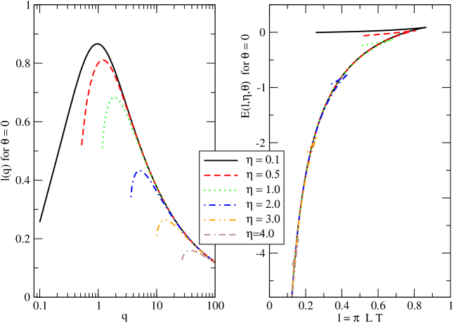
Figure 8: Same as Fig. 2, but now for dipole orientation $\theta=0$. Note that solutions with $\theta=0$ exist only for $q>\sinh\eta$.

Let us return to the case with $\theta=p=0$ keeping $q>\sinh\eta$. The solution evidently has $w^{\prime}=0$ throughout. Furthermore, although there is no reason of symmetry to expect it, given the wind blowing in the $x_{3}$ direction, we can see that the solution $y(\sigma)$ will be $\sigma\rightarrow-\sigma$ symmetric. This follows from the fact that $y^{\prime 2}$ depends only on $y$, not explicitly on $\sigma$, and from the symmetric boundary condition (153). This means that the descending half of the $y(\sigma)$ curve and the ascending half must have the same shape, implying that the turning point at which $y=y_{c}$ must be at $\sigma=0$, half way between the boundaries at which the boundary condition (153) fixes $y$. $q$ can be determined in terms of $l$ from (161), which with $p=0$ is simply the equation ${l\over 2}=\int^{l\over 2}_{0}d{\sigma}$ and becomes

$${l}={2q}\int_{y_{c}}^{{\Lambda}}dy\,{\sqrt{y^{4}-\cosh^{2}\eta}\over(y^{4}-1)\sqrt{(y^{4}-y_{c}^{4})}}\ ,$$ (164)

with $y_{c}$ given by (162). The action can be written as

$$S(l)=\sqrt{\lambda}T{\cal T}\int_{y_{c}}^{\Lambda}dy\;{\sqrt{y^{4}-\cosh^{2}\eta}\over\sqrt{y^{4}-y_{c}^{4}}}\ ,$$ (165)

from which the quark-antiquark potential $E(L)$ can be obtained as in (45) using the same subtraction $S_{0}$ given in (46). In plotting Fig. 8, we have used (164) and (165) to evaluate $l$ and $E$ for $q>\sinh\eta$. We see that the stable, lower energy branch of solutions is similar to those we have obtained previously. For this branch of solutions, the $\theta\rightarrow 0$ limit is smooth. The inaccessible range of $q$, namely $q<\sinh\eta$, where as described above the string world sheet develops a cusp in the $\theta\rightarrow 0$ limit, corresponds to the “missing parts” of the unstable high energy branch of solutions in Fig. 8.

References

- [1] K. Adcox et al. [PHENIX Collaboration], Nucl. Phys. A 757, 184 (2005) [arXiv:nucl-ex/0410003]; B. B. Back et al. [PHOBOS Collaboration], Nucl. Phys. A 757, 28 (2005) [arXiv:nucl-ex/0410022]; I. Arsene et al. [BRAHMS Collaboration]; Nucl. Phys. A 757, 1 (2005) [arXiv:nucl-ex/0410020]; J. Adams et al. [STAR Collaboration], Nucl. Phys. A 757, 102 (2005) [arXiv:nucl-ex/0501009].
- [2] J. M. Maldacena, Adv. Theor. Math. Phys. 2, 231 (1998) [Int. J. Theor. Phys. 38, 1113 (1999)] [arXiv:hep-th/9711200]; E. Witten, Adv. Theor. Math. Phys. 2, 253 (1998) [arXiv:hep-th/9802150]; S. S. Gubser, I. R. Klebanov and A. M. Polyakov, Phys. Lett. B 428, 105 (1998) [arXiv:hep-th/9802109]; O. Aharony, S. S. Gubser, J. M. Maldacena, H. Ooguri and Y. Oz, Phys. Rept. 323, 183 (2000) [arXiv:hep-th/9905111].
- [3] G. Policastro, D. T. Son and A. O. Starinets, Phys. Rev. Lett. 87, 081601 (2001) [arXiv:hep-th/0104066].
- [4] P. Kovtun, D. T. Son and A. O. Starinets, JHEP 0310, 064 (2003) [arXiv:hep-th/0309213].
- [5] A. Buchel and J. T. Liu, Phys. Rev. Lett. 93, 090602 (2004) [arXiv:hep-th/0311175].
- [6] A. Buchel, Nucl. Phys. B 708, 451 (2005) [arXiv:hep-th/0406200].
- [7] A. Buchel, J. T. Liu and A. O. Starinets, Nucl. Phys. B 707, 56 (2005) [arXiv:hep-th/0406264].
- [8] A. Buchel, Phys. Lett. B 609, 392 (2005) [arXiv:hep-th/0408095].
- [9] J. Mas, JHEP 0603, 016 (2006) [arXiv:hep-th/0601144]; D. T. Son and A. O. Starinets, JHEP 0603, 052 (2006) [arXiv:hep-th/0601157]; O. Saremi, arXiv:hep-th/0601159; K. Maeda, M. Natsuume and T. Okamura, Phys. Rev. D 73, 066013 (2006) [arXiv:hep-th/0602010].
- [10] P. Benincasa, A. Buchel and R. Naryshkin, arXiv:hep-th/0610145.
- [11] D. Teaney, Phys. Rev. C 68, 034913 (2003) [arXiv:nucl-th/0301099].
- [12] G. Policastro, D. T. Son and A. O. Starinets, JHEP 0209, 043 (2002) [arXiv:hep-th/0205052]. G. Policastro, D. T. Son and A. O. Starinets, JHEP 0212, 054 (2002) [arXiv:hep-th/0210220].
- [13] D. Teaney, arXiv:hep-ph/0602044; P. Kovtun and A. Starinets, Phys. Rev. Lett. 96, 131601 (2006) [arXiv:hep-th/0602059].
- [14] S. J. Sin and I. Zahed, Phys. Lett. B 608, 265 (2005) [arXiv:hep-th/0407215]; H. Nastase, arXiv:hep-th/0501068; E. Shuryak, S. J. Sin and I. Zahed, arXiv:hep-th/0511199; H. Nastase, arXiv:hep-th/0603176; S. Lin and E. Shuryak, arXiv:hep-ph/0610168; J. J. Friess, S. S. Gubser, G. Michalogiorgakis and S. S. Pufu, arXiv:hep-th/0611005.
- [15] H. Liu, K. Rajagopal and U. A. Wiedemann, Phys. Rev. Lett. 97, 182301 (2006) [arXiv:hep-ph/0605178].
- [16] A. Buchel, arXiv:hep-th/0605178.
- [17] J. F. Vazquez-Poritz, arXiv:hep-th/0605296.
- [18] E. Caceres and A. Guijosa, arXiv:hep-th/0606134.
- [19] F. L. Lin and T. Matsuo, arXiv:hep-th/0606136.
- [20] S. D. Avramis and K. Sfetsos, arXiv:hep-th/0606190.
- [21] N. Armesto, J. D. Edelstein and J. Mas, JHEP 0609, 039 (2006) [arXiv:hep-ph/0606245].
- [22] E. Nakano, S. Teraguchi and W. Y. Wen, arXiv:hep-ph/0608274.
- [23] C. P. Herzog, A. Karch, P. Kovtun, C. Kozcaz and L. G. Yaffe, JHEP 0607, 013 (2006) [arXiv:hep-th/0605158].
- [24] S. S. Gubser, arXiv:hep-th/0605182.
- [25] J. Casalderrey-Solana and D. Teaney, Phys. Rev. D 74, 085012 (2006) [arXiv:hep-ph/0605199].
- [26] C. P. Herzog, JHEP 0609, 032 (2006) [arXiv:hep-th/0605191]; E. Caceres and A. Guijosa, arXiv:hep-th/0605235; S. J. Sin and I. Zahed, arXiv:hep-ph/0606049. Y. h. Gao, W. s. Xu and D. f. Zeng, arXiv:hep-th/0606266; T. Matsuo, D. Tomino and W. Y. Wen, JHEP 0610, 055 (2006) [arXiv:hep-th/0607178];
- [27] J. J. Friess, S. S. Gubser and G. Michalogiorgakis, JHEP 0609, 072 (2006) [arXiv:hep-th/0605292]; J. J. Friess, S. S. Gubser, G. Michalogiorgakis and S. S. Pufu, arXiv:hep-th/0607022.
- [28] S. J. Rey, S. Theisen and J. T. Yee, Nucl. Phys. B 527, 171 (1998) [arXiv:hep-th/9803135]; A. Brandhuber, N. Itzhaki, J. Sonnenschein and S. Yankielowicz, Phys. Lett. B 434, 36 (1998) [arXiv:hep-th/9803137]; J. Sonnenschein, arXiv:hep-th/0003032.
- [29] D. Mateos, R. C. Myers and R. M. Thomson, Phys. Rev. Lett. 97, 091601 (2006) [arXiv:hep-th/0605046].
- [30] K. Peeters, J. Sonnenschein and M. Zamaklar, arXiv:hep-th/0606195.
- [31] H. Liu, K. Rajagopal and U. A. Wiedemann, arXiv:hep-ph/0607062.
- [32] M. Chernicoff, J. A. Garcia and A. Guijosa, JHEP 0609, 068 (2006) [arXiv:hep-th/0607089].
- [33] E. Caceres, M. Natsuume and T. Okamura, JHEP 0610, 011 (2006) [arXiv:hep-th/0607233].
- [34] P. C. Argyres, M. Edalati and J. F. Vazquez-Poritz, arXiv:hep-th/0608118.
- [35] S. D. Avramis, K. Sfetsos and D. Zoakos, arXiv:hep-th/0609079.
- [36] J. J. Friess, S. S. Gubser, G. Michalogiorgakis and S. S. Pufu, arXiv:hep-th/0609137.
- [37] P. Talavera, arXiv:hep-th/0610179.
- [38] M. Chernicoff and A. Guijosa, arXiv:hep-th/0611155.
- [39] See also Appendix A of Ref. [23].
- [40] K. G. Wilson, Phys. Rev. D 10, 2445 (1974).
- [41] L. D. McLerran and B. Svetitsky, Phys. Lett. B 98, 195 (1981); J. Kuti, J. Polonyi and K. Szlachanyi, Phys. Lett. B 98, 199 (1981); L. D. McLerran and B. Svetitsky, Phys. Rev. D 24, 450 (1981).
- [42] O. Philipsen, Phys. Lett. B 535 (2002) 138 [arXiv:hep-lat/0203018]; O. Jahn and O. Philipsen, Phys. Rev. D 70, 074504 (2004) [arXiv:hep-lat/0407042].
- [43] O. Kaczmarek, F. Karsch, P. Petreczky and F. Zantow, Phys. Lett. B 543 (2002) 41 [arXiv:hep-lat/0207002].
- [44] M. Laine, O. Philipsen, P. Romatschke and M. Tassler, arXiv:hep-ph/0611300.
- [45] J. M. Maldacena, Phys. Rev. Lett. 80, 4859 (1998) [arXiv:hep-th/9803002]; S. J. Rey and J. T. Yee, Eur. Phys. J. C 22, 379 (2001) [arXiv:hep-th/9803001].
- [46] T. Matsui and H. Satz, Phys. Lett. B 178, 416 (1986).
- [47] H. Satz, J. Phys. G 32 (2006) R25 [arXiv:hep-ph/0512217].
- [48] A. Kovner and U. A. Wiedemann, Phys. Rev. D 64, 114002 (2001) [arXiv:hep-ph/0106240].
- [49] A. Kovner and U. A. Wiedemann, arXiv:hep-ph/0304151.
- [50] A. H. Mueller, Nucl. Phys. B 335 (1990) 115.
- [51] N. N. Nikolaev and B. G. Zakharov, Z. Phys. C 49, 607 (1991).
- [52] G. Piller and W. Weise, Phys. Rept. 330, 1 (2000) [arXiv:hep-ph/9908230].
- [53] Y. V. Kovchegov and L. D. McLerran, Phys. Rev. D 60 (1999) 054025 [Erratum-ibid. D 62 (2000) 019901] [arXiv:hep-ph/9903246].
- [54] U. A. Wiedemann, Nucl. Phys. B 582, 409 (2000) [arXiv:hep-ph/0003021].
- [55] A. Kovner, Acta Phys. Polon. B 36 (2005) 3551 [arXiv:hep-ph/0508232].
- [56] H. Weigert, Prog. Part. Nucl. Phys. 55 (2005) 461 [arXiv:hep-ph/0501087].
- [57] E. Iancu and R. Venugopalan, arXiv:hep-ph/0303204.
- [58] J. W. Cronin et al., Phys. Rev. D 11, 3105 (1975), S. S. Adler et al. [PHENIX Collaboration], Phys. Rev. Lett. 91 (2003) 072303 [arXiv:nucl-ex/0306021], J. Adams et al. [STAR Collaboration], Phys. Rev. Lett. 91 (2003) 072304 [arXiv:nucl-ex/0306024], B. B. Back et al. [PHOBOS Collaboration], Phys. Rev. Lett. 91 (2003) 072302 [arXiv:nucl-ex/0306025], I. Arsene et al. [BRAHMS Collaboration], Phys. Rev. Lett. 91 (2003) 072305 [arXiv:nucl-ex/0307003].
- [59] D. Kharzeev, E. Levin and L. McLerran, Phys. Lett. B 561, 93 (2003) [arXiv:hep-ph/0210332].
- [60] R. Baier, A. Kovner and U. A. Wiedemann, Phys. Rev. D 68 (2003) 054009 [arXiv:hep-ph/0305265].
- [61] D. Kharzeev, Y. V. Kovchegov and K. Tuchin, Phys. Rev. D 68 (2003) 094013 [arXiv:hep-ph/0307037].
- [62] J. L. Albacete, N. Armesto, A. Kovner, C. A. Salgado and U. A. Wiedemann, Phys. Rev. Lett. 92 (2004) 082001 [arXiv:hep-ph/0307179].
- [63] J. Jalilian-Marian, Y. Nara and R. Venugopalan, Phys. Lett. B 577, 54 (2003) [arXiv:nucl-th/0307022].
- [64] J. P. Blaizot, F. Gelis and R. Venugopalan, Nucl. Phys. A 743 (2004) 13 [arXiv:hep-ph/0402256].
- [65] Y. V. Kovchegov and A. H. Mueller, Nucl. Phys. B 529 (1998) 451 [arXiv:hep-ph/9802440].
- [66] R. Baier, Nucl. Phys. A 715, 209 (2003) [arXiv:hep-ph/0209038].
- [67] R. Baier, Y. L. Dokshitzer, A. H. Mueller, S. Peigne and D. Schiff, Nucl. Phys. B 484 (1997) 265 [arXiv:hep-ph/9608322].
- [68] B. G. Zakharov, JETP Lett. 63 (1996) 952 [arXiv:hep-ph/9607440]; JETP Lett. 65, 615 (1997) [arXiv:hep-ph/9704255].
- [69] U. A. Wiedemann, Nucl. Phys. B 588, 303 (2000) [arXiv:hep-ph/0005129].
- [70] B. Z. Kopeliovich, A. V. Tarasov and A. Schafer, Phys. Rev. C 59 (1999) 1609 [arXiv:hep-ph/9808378].
- [71] W. Buchmuller and A. Hebecker, Nucl. Phys. B 476 (1996) 203 [arXiv:hep-ph/9512329].
- [72] C. A. Salgado and U. A. Wiedemann, Phys. Rev. Lett. 93, 042301 (2004) [arXiv:hep-ph/0310079].
- [73] C. A. Salgado and U. A. Wiedemann, Phys. Rev. D 68 (2003) 014008 [arXiv:hep-ph/0302184].
- [74] B. G. Zakharov, JETP Lett. 73, 49 (2001) [Pisma Zh. Eksp. Teor. Fiz. 73, 55 (2001)] [arXiv:hep-ph/0012360].
- [75] M. Gyulassy, P. Levai and I. Vitev, Nucl. Phys. B 594, 371 (2001) [arXiv:nucl-th/0006010]; X. N. Wang and X. f. Guo, Nucl. Phys. A 696, 788 (2001) [arXiv:hep-ph/0102230]; S. Jeon and G. D. Moore, Phys. Rev. C 71, 034901 (2005) [arXiv:hep-ph/0309332].
- [76] For reviews, see R. Baier, D. Schiff and B. G. Zakharov, Ann. Rev. Nucl. Part. Sci. 50, 37 (2000) [arXiv:hep-ph/0002198]; M. Gyulassy, I. Vitev, X. N. Wang and B. W. Zhang, arXiv:nucl-th/0302077; P. Jacobs and X. N. Wang, Prog. Part. Nucl. Phys. 54, 443 (2005) [arXiv:hep-ph/0405125].
- [77] F. Carminati et al. [ALICE Collaboration], J. Phys. G 30, 1517 (2004); G. Baur et al. [CMS Collaboration], CMS-Note-2000-060; H. Takai, [for the ATLAS Collaboration] Eur. Phys. J. C 34, S307 (2004).
- [78] R. Baier and D. Schiff, JHEP 0609, 059 (2006) [arXiv:hep-ph/0605183].
- [79] L. Susskind and E. Witten, arXiv:hep-th/9805114; A. W. Peet and J. Polchinski, Phys. Rev. D 59, 065011 (1999) [arXiv:hep-th/9809022].
- [80] E. Witten, in Ref. [2]
- [81] F. Karsch, D. Kharzeev and H. Satz, Phys. Lett. B 637, 75 (2006) [arXiv:hep-ph/0512239].
- [82] S. Digal, P. Petreczky and H. Satz, Phys. Lett. B 514, 57 (2001); H. Satz, arXiv:hep-ph/0609197.
- [83] F. Karsch and R. Petronzio, Z. Phys. C 37, 627 (1988).
- [84] N. Armesto, C. A. Salgado and U. A. Wiedemann, Phys. Rev. C 72, 064910 (2005) [arXiv:hep-ph/0411341].
- [85] T. Renk and J. Ruppert, Phys. Rev. C 72, 044901 (2005) [arXiv:hep-ph/0507075].
- [86] R. Baier, private communication, R. Baier, A. H. Mueller and D. Schiff, arXiv:nucl-th/0612068.
- [87] T. Renk, J. Ruppert, C. Nonaka and S. A. Bass, arXiv:nucl-th/0611027.
- [88] I. R. Klebanov and M. J. Strassler, JHEP 0008, 052 (2000) [arXiv:hep-th/0007191].
- [89] For recent reviews, see J. Phys. Conf. Ser. 46, 122 (2006) [arXiv:hep-lat/0608003]; F. Karsch, arXiv:hep-ph/0610024.
- [90] S. Caron-Huot, P. Kovtun, G. D. Moore, A. Starinets and L. G. Yaffe, arXiv:hep-th/0607237; S. C. Huot, S. Jeon and G. D. Moore, arXiv:hep-ph/0608062.
- [91] S. S. Gubser, arXiv:hep-th/0611272.
- [92] F. Karsch, Nucl. Phys. A 698, 199 (2002) [arXiv:hep-ph/0103314].
- [93] S. S. Gubser, I. R. Klebanov and A. W. Peet, Phys. Rev. D 54, 3915 (1996) [arXiv:hep-th/9602135].
- [94] S. S. Gubser, I. R. Klebanov and A. A. Tseytlin, Nucl. Phys. B 534, 202 (1998) [arXiv:hep-th/9805156].
- [95] B. Bringoltz and M. Teper, Phys. Lett. B 628, 113 (2005) [arXiv:hep-lat/0506034].
- [96] K. J. Eskola et al., Nucl. Phys. A 747, 511 (2005) [arXiv:hep-ph/0406319].
- [97] A. Dainese, C. Loizides and G. Paic, Eur. Phys. J. C 38, 461 (2005) [arXiv:hep-ph/0406201].
- [98] P. F. Kolb and U. W. Heinz, arXiv:nucl-th/0305084.
- [99] G. D. Moore and D. Teaney, Phys. Rev. C 71, 064904 (2005) [arXiv:hep-ph/0412346].
- [100] J. Casalderrey-Solana, private communication.
- [101] F. Karsch, E. Laermann and A. Peikert, Phys. Lett. B 478, 447 (2000) [arXiv:hep-lat/0002003].
- [102] G. Boyd, J. Engels, F. Karsch, E. Laermann, C. Legeland, M. Lutgemeier and B. Petersson, Nucl. Phys. B 469, 419 (1996) [arXiv:hep-lat/9602007].
- [103] A. Ali Khan et al. [CP-PACS collaboration], Phys. Rev. D 64, 074510 (2001) [arXiv:hep-lat/0103028].
- [104] Y. Aoki, Z. Fodor, S. D. Katz and K. K. Szabo, JHEP 0601, 089 (2006) [arXiv:hep-lat/0510084].
- [105] S. Ejiri, F. Karsch, E. Laermann and C. Schmidt, Phys. Rev. D 73, 054506 (2006) [arXiv:hep-lat/0512040].
- [106] O. Kaczmarek, F. Karsch, F. Zantow and P. Petreczky, Phys. Rev. D 70, 074505 (2004) [Erratum-ibid. D 72, 059903 (2005)] [arXiv:hep-lat/0406036].
- [107] O. Kaczmarek and F. Zantow, Phys. Rev. D 71, 114510 (2005) [arXiv:hep-lat/0503017].
- [108] A. Muronga, Phys. Rev. Lett. 88 (2002) 062302 [Erratum-ibid. 89 (2002) 159901] [arXiv:nucl-th/0104064]; A. Muronga, Phys. Rev. C 69 (2004) 034903 [arXiv:nucl-th/0309055]; U. W. Heinz, H. Song and A. K. Chaudhuri, Phys. Rev. C 73 (2006) 034904 [arXiv:nucl-th/0510014]; R. Baier, P. Romatschke and U. A. Wiedemann, Phys. Rev. C 73 (2006) 064903 [arXiv:hep-ph/0602249]; R. Baier and P. Romatschke, arXiv:nucl-th/0610108.
- [109] J. P. Gauntlett, D. Martelli, J. Sparks and D. Waldram, Adv. Theor. Math. Phys. 8, 711 (2004) [arXiv:hep-th/0403002].
- [110] S. Benvenuti, S. Franco, A. Hanany, D. Martelli and J. Sparks, JHEP 0506, 064 (2005) [arXiv:hep-th/0411264].
- [111] I. R. Klebanov and E. Witten, Nucl. Phys. B 536, 199 (1998) [arXiv:hep-th/9807080].
- [112] M. Henningson and K. Skenderis, JHEP 9807, 023 (1998) [arXiv:hep-th/9806087].
- [113] S. S. Gubser, Phys. Rev. D 59, 025006 (1999) [arXiv:hep-th/9807164].
- [114] K. Pilch and N. P. Warner, Phys. Lett. B 487, 22 (2000) [arXiv:hep-th/0002192].
- [115] R. G. Leigh and M. J. Strassler, Nucl. Phys. B 447, 95 (1995) [arXiv:hep-th/9503121].
- [116] J. P. Gauntlett, D. Martelli, J. Sparks and D. Waldram, Class. Quant. Grav. 23, 4693 (2006) [arXiv:hep-th/0510125].
- [117] D. Z. Freedman, S. S. Gubser, K. Pilch and N. P. Warner, Adv. Theor. Math. Phys. 3, 363 (1999) [arXiv:hep-th/9904017].
- [118] A. Buchel and J. T. Liu, JHEP 0311, 031 (2003) [arXiv:hep-th/0305064].
- [119] N. Itzhaki, J. M. Maldacena, J. Sonnenschein and S. Yankielowicz, Phys. Rev. D 58, 046004 (1998) [arXiv:hep-th/9802042].
- [120] S. S. Gubser, arXiv:hep-th/0612143.
- [121] J. Casalderrey-Solana and D. Teaney, arXiv:hep-th/0701123.
- [122] P. C. Argyres, M. Edalati and J. F. Vazquez-Poritz, arXiv:hep-th/0612157.
- [123] Y. L. Dokshitzer and D. E. Kharzeev, Phys. Lett. B 519 (2001) 199 [arXiv:hep-ph/0106202]; N. Armesto, C. A. Salgado and U. A. Wiedemann, Phys. Rev. D 69 (2004) 114003 [arXiv:hep-ph/0312106].