The Higgs effective potential in the Littlest Higgs model at the one-loop level

Abstract

In this work we compute the contributions to the Higgs effective potential coming from the fermion and gauge boson sectors at the one-loop level in the context of the $SU(5)/SO(5)$ Littlest Higgs (LH) model using a cutoff $\Lambda$ and including all finite parts. We consider both, the $(SU(2)\times U(1))_{1}\times(SU(2)\times U(1))_{2}$ and the $(SU(2)\times U(1))_{1}\times(SU(2)\times U(1))$ gauge group versions of the LH model. We also show that the Goldstone bosons present in the model do not contribute to the effective potential at the one-loop level. Finally, by neglecting the contribution of higher dimensional operators, we discuss the restrictions that the new one-loop contributions set on the parameter space of the LH model and the need to include higher loop corrections to the Higgs potential.

I Introduction

The quadratically divergent contributions to the Higgs mass and the electroweak precision observables imply different scales for physics beyond the Standard Model (SM), the first one below $2$ TeV and the second above $10$ TeV. This is the so called little hierarchy problem. An interesting attempt to solve it, inspired in an old suggestion by Georgi and Pais Georgi , is the Littlest Higgs model (LH) Cohen which is based on a $SU(5)/SO(5)$ non-sigma linear model (see Schmaltz and review1 for recent reviews). Being a Goldstone boson (GB) associated to this spontaneous symmetry breaking, the Higgs is massless in principle. However one-loop corrections produce a logarithmically divergent Higgs mass that could be compatible with the present experimental bound of about $200$ GeV. The others GB present in the model get quadratically divergent masses at the one-loop level becoming very massive or give masses to the SM and other additional gauge bosons present in the model through the Higgs mechanism. All of these new states could give rise to a very rich phenomenology that could be proved at the CERN Large Hadron Collider (LHC) Logan .

From the LH model it is possible, at least in principle, to compute the Higgs low-energy effective potential. Obviously this effective potential should reproduce the form of the SM potential, i.e.:

$$V_{eff}(H)=-\mu^{2}HH^{{\dagger}}+\lambda(HH^{{\dagger}})^{2},$$ (1)

where $H=(H^{0},H^{+})$ is the SM Higgs doublet and $\mu^{2}$ and $\lambda$ are the well known Higgs mass and Higgs selfcoupling parameters. Notice that, in order to have spontaneous symmetry breaking of the electroweak symmetry, $\mu^{2}$ must be negative and $\lambda$ must be positive to have a well defined energy minimum. In addition these parameters should reproduce the SM relation $m_{H}^{2}=2\lambda v^{2}=2\mu^{2}$ where $m_{H}$ is the Higgs mass and $v$ is the vacuum expectation value (vev).

In principle $\mu^{2}$ and $\lambda$ receive contributions from fermion, gauge boson and scalar loops, besides others that could come from the ultraviolet completion of the LH model italianos . In this work we continue our program consisting in the computation of the relevant terms of the Higgs low-energy effective potential and their phenomenological consequences including new restrictions on the parameter space of the LH model.

In particular we will study the consistency of the electroweak symmetry breaking with the present experimental data in the case in which, for the sake of simplicity, one neglects the contribution of higher dimensional operators coming from the ultraviolet completion of the LH model that are generically present.

In ATP we obtained the (one-loop) contribution coming from the third generation quarks $t$ and $b$ plus the $T$ quark present in the LH model. This contribution is essential since it provides the right positive sign for $\mu^{2}$ being other contributions negative. Here we complete the one-loop computation of the Higgs potential by including also gauge bosons and clarifying the role of the GB at this level. We also discuss the validity of the one-loop potential and the necessity of including some important higher loop contributions to reproduce the expected value of the Higgs mass.

The paper is organized as follows: In Section 2 we briefly review the LH model and set the notation. In section 3 we study the LH model as a gauged non-linear sigma model (NLSM). In particular we pay attention to the problem of the quartic divergencies appearing when a cutoff $\Lambda$ is used to regulate the divergences of the model and we show how they cancel at the one-loop level. We also obtain the gauge fixing and Faddeev-Popov terms appropriate for the calculation of the different gauge boson loops appearing latter in our computations. In Section 4 we compute the effective potential at the one-loop level. Section 5 is devoted to a discussion of our results and the constraints that our computation establishes on the LH parameters. Finally, in Section 6 we present the main conclusions of this paper and the prospects for future work.

II Setting of the Littlest Higgs model

As it is well know the low energy dynamics of the LH model can be described by a $(SU(2)\times U(1))_{1}\times(SU(2)\times U(1))_{2}$ gauged non-linear sigma model based on the coset $K=G/H=SU(5)/SO(5)$. The Goldstone boson fields can be disposed in a $5\times 5$ matrix $\Sigma$ given by:

$$\Sigma=e^{2i\Pi/f}\Sigma_{0},$$ (2)

where:

$$\Sigma_{0}=\left(\begin{array}[]{ccc}0&0&\textbf{1}\\ 0&1&0\\ \textbf{1}&0&0\\ \end{array}\right)$$ (3)

has the proper $SU(5)$ symmetry breaking structure with 1 being the $2\times 2$ unit matrix, and

$$\Pi = \left(\begin{array}[]{ccc}\xi&\frac{-i}{\sqrt{2}}H^{{\dagger}}&\phi^{{\dagger}}\\ \frac{i}{\sqrt{2}}H&0&\frac{-i}{\sqrt{2}}H^{*}\\ \phi&\frac{i}{\sqrt{2}}H^{T}&\xi^{T}\\ \end{array}\right)$$

$$+ \frac{1}{\sqrt{20}}\,\eta\,{\mbox{diag }}(1,1,-4,1,1).\,,$$

Here $H=(H^{0},H^{+})$ is the SM Higgs doublet, $\eta$ is the real scalar and $\xi$ and $\phi$ are the real triplet and the complex triplet respectively:

$$\xi=\left(\begin{array}[]{cc}\frac{1}{2}\xi^{0}&\frac{1}{\sqrt{2}}\xi^{+}\\ \frac{1}{\sqrt{2}}\xi^{-}&-\frac{1}{2}\xi^{0}\end{array}\right)\,,$$ (8)

and

$$\phi=\left(\begin{array}[]{cc}\phi^{0}&\frac{1}{\sqrt{2}}\phi^{+}\\ \frac{1}{\sqrt{2}}\phi^{+}&\phi^{++}\end{array}\right)\,.$$ (9)

The gauged non-linear sigma model lagrangian describing the low-energy GB and gauge boson dynamics is given by:

$$\textit{L}_{0}=\frac{f^{2}}{8}\mbox{tr}[(D_{\mu}\Sigma)(D^{\mu}\Sigma)^{\dagger}].$$ (10)

The covariant derivative is defined as:

$$D_{\mu}\Sigma = \partial_{\mu}\Sigma-i\sum_{j=1}^{2}g_{j}W^{a}_{j}(Q_{j}^{a}\Sigma+\Sigma Q_{j}^{aT})$$ (11)

$$- i\sum_{j=1}^{2}g^{\prime}_{j}B_{j}(Y_{j}\Sigma+\Sigma Y_{j}^{T})$$

where $g$ and $g^{\prime}$ are the gauge couplings, $Q_{1ij}^{a}=\sigma_{ij}^{a}/2$, for $i,j=1,2$, $Q_{2ij}^{a}=\sigma_{ij}^{a*}/2$ for $i,j=4,5$ and zero otherwise, $Y_{1}=diag(-3,-3,2,2,2)/10$ and $Y_{2}=diag(-2,-2,-2,3,3)/10$. Diagonalizing the gauge boson mass matrix in this Lagrangian one realizes that the $W$ and $B$ SM gauge bosons are massless and the $W^{\prime}$ and $B^{\prime}$ gauge bosons have masses:

$$M_{W^{\prime}}=f\sqrt{g_{1}^{2}+g_{2}^{2}}/2{\mbox{ ; }}M_{B^{\prime}}=f\sqrt{g_{1}^{{}^{\prime}2}+g_{2}^{{}^{\prime}2}}/\sqrt{20}.$$ (12)

The gauge bosons mass eigenstates are defined such as:

$$W^{a} = c_{\psi}W_{1}^{a}+s_{\psi}W_{2}^{a}$$

$$W^{{}^{\prime}a} = s_{\psi}W_{1}^{a}-c_{\psi}W_{2}^{a}$$ (13)

where

$$s_{\psi} = \sin\psi=\frac{g_{1}}{\sqrt{g_{1}^{2}+g_{2}^{2}}}$$

$$c_{\psi} = \cos\psi=\frac{g_{2}}{\sqrt{g_{1}^{2}+g_{2}^{2}}}$$ (14)

and

$$B = c^{\prime}_{\psi}B_{1}+s^{\prime}_{\psi}B_{2}$$

$$B^{\prime} = s^{\prime}_{\psi}B_{1}-c^{\prime}_{\psi}W_{2}$$ (15)

with

$$s^{\prime}_{\psi}=\sin\psi^{\prime}=\frac{g^{\prime}_{1}}{\sqrt{{g^{\prime}}_{1}^{\,2}+{g^{\prime}}_{2}^{\,2}}}$$

$$c^{\prime}_{\psi}=\cos\psi^{\prime}=\frac{{g^{\prime}}_{2}}{\sqrt{{g^{\prime}}_{1}^{\,2}+{g^{\prime}}_{2}^{\,2}}}\,.$$ (16)

A modified version of the LH model, such that the gauge subgroup of $SU(5)$ is $[SU(2)\times SU(2)\times U(1)_{Y}]$ rather than $[SU(2)\times U(1)_{Y}]^{2}$, has also been introduced Peskin . In this case, the covariant derivative is defined as:

$$D_{\mu}\Sigma=\partial_{\mu}\Sigma-i\sum_{j=1}^{2}g_{j}W^{a}_{j}(Q_{j}^{a}\Sigma+\Sigma Q_{j}^{aT})-ig^{\prime}B(Y\Sigma+\Sigma Y^{T})\,,$$ (17)

where the generators $Q_{j}^{a}$ are the same as in the previous case, and $Y=\frac{1}{2}$diag$(-1,-1,0,1,1)$. The field content of the matrix $\Pi$ in $\Sigma$ is the same as in the LH model but there is no $B^{{}^{\prime}}$ now. We consider in our analysis these two different models: the original LH with two $U(1)$ groups (Model I) and the other one with just one $U(1)$ group (Model II).

Then, at the tree level, the $SU(2)_{L}\times U(1)_{Y}$ SM gauge group remains unbroken. The spontaneously symmetry breaking of this group is expected to be produced in principle radiatively, mainly due to the effect of the virtual quark fields from the third generation, which give rise to an appropriate effective potential for the SM Higgs doublet. These quarks will initially be denoted by $u$ and $b$ and the additional vector-like quark will be denoted by $U$. The interactions between these fermions and the Goldstone bosons are given by the Yukawa Lagrangian:

$$\textit{L}_{YK}=-\frac{\lambda_{1}}{2}f\overline{u}_{R}\epsilon_{mn}\epsilon_{ijk}\Sigma_{im}\Sigma_{jn}\chi_{Lk}-\lambda_{2}f\overline{U}_{R}U_{L}+\mbox{h.c.},$$ (18)

where $m,n=4,5$, $i,j=1,2,3$, and

$$\overline{u}_{R} = c\,\overline{t}_{R}+s\,\overline{T}_{R}\,,$$

$$\overline{U}_{R} = -s\,\overline{t}_{R}+c\,\overline{T}_{R},$$ (19)

with:

$$c = \cos\theta=\frac{\lambda_{2}}{\sqrt{\lambda_{1}^{2}+\lambda_{2}^{2}}},$$

$$s = \sin\theta=\frac{\lambda_{1}}{\sqrt{\lambda_{1}^{2}+\lambda_{2}^{2}}}\,,$$ (20)

and

$$\chi_{L}=\left(\begin{array}[]{c}u\\ b\\ U\\ \end{array}\right)_{L}=\left(\begin{array}[]{c}t\\ b\\ T\\ \end{array}\right)_{L}.$$ (21)

Here $b\,,t$ and $T$ are the mass eigenvectors coming from the mass matrix included in the Yukawa Lagrangian with eigenvalues: $m_{t}=m_{b}=0$ and $m_{T}=f\sqrt{\lambda_{1}^{2}+\lambda_{2}^{2}}$. Notice that, contrary to the quark $T$ which is massive already at this level, the $t$ quark is massless and acquires mass only when the electroweak symmetry is broken.

Then, the Yukawa Lagrangian can be written as:

$$\textit{L}_{\rm{Yuk}}=\overline{\chi}_{R}\hat{I}_{3x3}\chi_{L}+\mbox{h.c.}\,,$$ (22)

with

$$\chi_{R}=\left(\begin{array}[]{c}t\\ b\\ T\\ \end{array}\right)_{R}$$

and $\hat{I}_{3x3}$ the Higgs-quark interaction matrix is given by

$$\hat{I}=\left(\begin{array}[]{ccc}-\sqrt{2}\lambda_{1}cH^{0}\Theta&-\sqrt{2}\lambda_{1}cH^{+}\Theta&\lambda_{1}c\frac{HH^{{\dagger}}}{f}\Theta^{{}^{\prime}}\\ 0&0&0\\ -\sqrt{2}\lambda_{1}sH^{0}\Theta&-\sqrt{2}\lambda_{1}sH^{+}\Theta&\lambda_{1}s\frac{HH^{{\dagger}}}{f}\Theta^{{}^{\prime}}\end{array}\right),$$ (26)

where $\Theta$ and $\Theta^{{}^{\prime}}$ are functions on $HH^{\dagger}/f^{2}$ whose expansion starts as:

$$\Theta\left(\frac{HH^{{\dagger}}}{f^{2}}\right)=1-\frac{2HH^{{\dagger}}}{3f^{2}}+...$$ (27)

$$\Theta^{\prime}\left(\frac{HH^{{\dagger}}}{f^{2}}\right)=1-\frac{HH^{{\dagger}}}{3f^{2}}+...$$

Thus the complete Lagrangian for the quarks is:

$$\textit{L}_{\chi} = \textit{L}_{0}+\textit{L}_{\rm{Yuk}}=\overline{\chi}_{R}(i{\partial\mkern-9.0mu/}-M+\hat{I})\chi_{L}+\mbox{h.c.}$$ (28)

with $M=$diag$(0,0,m_{T})$.

Since we are interested in the computation of the contribution to the SM Higgs $H$ effective potential, we can set $\xi=\phi=\eta=0$.

III The Littlest Higgs model as a Non linear sigma model

III.1 Quartic divergences

In order to compute the contributions to the Higgs potential coming from scalar and gauge boson loops it is useful to study the LH model as a particular case of gauged non-linear sigma model (NLSM) based on the coset $K=G/H=SU(5)/SO(5)$ (see  book for a review on gauged NLSM). To start with we will turn off the gauge interactions by taken $g_{i}^{(^{\prime})}=0$. Then the $\textit{L}_{0}$ lagrangian is:

$$\textit{L}_{0}=\frac{f^{2}}{8}\mbox{tr}[(\partial_{\mu}\Sigma)(\partial^{\mu}\Sigma)^{{\dagger}}]$$ (29)

This lagrangian can be written also as a NLSM lagrangian

$$\textit{L}_{0}=\frac{1}{2}g_{\alpha\beta}(\pi)\partial_{\mu}\pi^{\alpha}\partial^{\mu}\pi^{\beta}$$ (30)

where $\pi^{\alpha}$ are Gaussian coordinates on $K$ and the $K$ metric is defined as:

$$g_{\alpha\beta}\equiv\frac{f^{2}}{4}\mbox{tr}\frac{\partial\Sigma}{\partial\pi^{\alpha}}\frac{\partial\Sigma^{{\dagger}}}{\partial\pi^{\beta}}$$ (31)

This metric can be split as

$$g_{\alpha\beta}=\delta_{\alpha\beta}+\Delta_{\alpha\beta}(\pi)$$ (32)

where

$$\Delta_{ab}(\pi) = -\frac{8}{3!f^{2}}\mbox{tr}(T_{\alpha}T_{\beta}T_{\delta}T_{\gamma}+T_{\alpha}T_{\delta}T_{\beta}T_{\gamma}$$ (33)

$$+ T_{\alpha}T_{\delta}T_{\gamma}T_{\beta})\pi_{\delta}\pi_{\gamma}+\textit{O}(\pi^{4})$$

$$= -\frac{8}{3!f^{2}}\kappa_{\alpha\beta\delta\gamma}\pi_{\delta}\pi_{\gamma}+\textit{O}(\pi^{4})$$

and we have written $\Pi$ as $\Pi=\pi^{\alpha}T^{\alpha}$ with the $T^{\alpha}$ matrices normalized so that tr$T^{\alpha}T^{\beta}=\delta^{\alpha\beta}$. Now we consider the coupling of the NLSM with any other field $\phi$ which for simplicity will be taken to be a real scalar. The corresponding action can be written as $S[\pi,\phi]=S_{0}[\pi]+S^{\prime}[\pi,\phi]$. The effective action for the $\phi$ field can be obtained by integrating out the GB fields $\pi$. However this integration is not trivial at all. Due to the geometrical nature of the NLSM, not only its action, but also the integration measure, must be $G$ invariant and covariant in the $K$ coset sense measure . Thus the proper $\phi$ effective action is given by:

$$e^{i\Gamma[\phi]}=\int[d\pi\sqrt{g}]e^{iS[\pi,\phi]}$$ (34)

The measure factor $\sqrt{g}$ can now be exponentiated to find

$$e^{i\Gamma[\phi]}=\int[d\pi]e^{i(S[\pi,\phi]+\Delta\Gamma[\pi])}$$ (35)

with

$$\Delta\Gamma[\pi] = -\frac{i}{2}\delta(0)\int dx\log(1+\Delta)$$ (36)

$$= -\frac{i}{2}\delta(0)\Sigma_{k=1}^{\infty}\frac{(-1)^{k+1}}{k}\int dx\mbox{tr}\Delta^{k}$$

where by using the notation $d\tilde{k}\equiv d^{D}k/(2\pi)^{D}$ with $D$ being the space-time dimensionality so that:

$$\delta(0)=\int d\tilde{k}$$ (37)

In the dimensional regularization scheme one has

$$\delta(0)=\int\frac{d^{D}k}{(2\pi)^{D}}=0$$ (38)

but using an ultraviolet cutoff $\Lambda$ to define divergent integrals

$$\delta(0)=\int d\tilde{k}=i\frac{\Lambda^{4}}{2(4\pi)^{2}}$$ (39)

which obviously does not vanish. Then, in order to take into account the invariant measure effects in the NLSM one needs to add to the classical lagrangian the term

$$S_{0}\rightarrow S_{0}+\Delta\Gamma$$ (40)

whenever one is not using dimensional regularization. It is not difficult to see that this term is formally of the same order as the one-loop contributions.

On the other hand the GB contribution to the Higgs effective potential is defined as

$$\Gamma_{eff}[\overline{\pi}]=-\int dxV_{eff}(\overline{\pi})$$ (41)

where $\overline{\pi}$ is a constant field and

$$e^{i\Gamma_{eff}[\overline{\pi}]}=\int[d\pi^{\prime}\sqrt{g}]e^{iS_{0}[\overline{\pi}+\pi^{\prime}]}$$ (42)

with

$$\frac{\delta\Gamma_{eff}[\pi]}{\delta\pi}|_{\pi=\overline{\pi}}=0$$ (43)

At the one-loop level the last equation can be written as

$$\frac{\delta S_{0}[\pi]}{\delta\pi}|_{\pi=\overline{\pi}}\simeq 0$$ (44)

and then the NLSM action can be expanded as

$$S_{0}[\overline{\pi}+\pi^{\prime}] = S_{0}[\overline{\pi}]$$

$$+ \frac{1}{2}\int dxdy\pi^{\prime\alpha}(x)\frac{\delta^{2}S_{0}}{\delta\pi^{\alpha}(x)\delta\pi^{\beta}(y)}\Big{|}_{\pi=\overline{\pi}}\pi^{\prime\beta}(y)$$

Therefore we have

$$\Gamma_{eff}[\overline{\pi}]=S_{0}[\overline{\pi}]+\frac{i}{2}\mbox{Tr log}(1+GO)+...$$ (46)

where the inverse GB propagator is

$$(G_{xy}^{\alpha\beta})^{-1}=-\Box_{x}\delta_{xy}\delta_{\alpha\beta}$$ (47)

$\delta_{xy}$ being the short for $\delta(x-y)$ and

$$O_{xy}^{\alpha\beta}=\frac{\delta^{2}}{\delta\pi^{\alpha}(x)\delta\pi^{\beta}(y)}\int dx\partial_{\mu}\pi^{\alpha}\Delta_{\alpha\beta}(\pi)\partial^{\mu}\pi^{\beta}\Big{|}_{\pi=\overline{\pi}}$$ (48)

In order to compute the Higgs effective action we only need to consider the case $\overline{\pi}=$cte which means $\partial_{\mu}\overline{\pi}=0$ and then we have

$$O_{xy}^{\alpha\beta}(\pi)=-\Delta_{\alpha\beta}(\overline{\pi})\Box_{x}\delta_{xy}.$$ (49)

Therefore we get

$$\Gamma_{eff}[\overline{\pi}]=\frac{i}{2}\mbox{Tr}\Sigma_{k=1}^{\infty}\frac{(-1)^{k+1}}{k}(OG)^{k}+...$$ (50)

or

$$\Gamma_{eff}[\overline{\pi}]=\frac{i}{2}\delta(0)\int dx\mbox{tr}\left(\Delta-\frac{\Delta^{2}}{2}+\frac{\Delta^{3}}{3}+...\right)+...$$ (51)

This effective action has exactly the same form as the measure term discussed above so finally we get:

$$\Gamma_{eff}[\overline{\pi}]+\Delta\Gamma[\overline{\pi}]=0$$ (52)

Therefore we arrive to the important conclusion that the GB do not contribute to the Higgs potential in any NLSM at the one loop level and in particular this is the case for the $SU(5)/SO(5)$ LH model.

III.2 Gauge fixing and the Faddeev-Popov terms

In the following we will concentrate on the gauge bosons in order to be able to compute their contribution to the Higgs effective potential. Thus we turn on again the gauge boson fields in the NLSM:

$$\textit{L}_{0}=\frac{f^{2}}{8}\mbox{tr}[(D_{\mu}\Sigma)(D_{\mu}\Sigma)^{{\dagger}}]$$ (53)

The covariant derivative can be written in terms of the mass eigenstates as:

$$D_{\mu}\Sigma = \partial_{\mu}\Sigma-igW^{a}_{\mu}(Q^{a}_{L}\Sigma+\Sigma Q_{L}^{aT})$$ (54)

$$- ig_{R}W^{\prime a}_{\mu}(Q^{a}_{R}\Sigma+\Sigma Q_{R}^{aT})-ig^{\prime}B_{\mu}(Y\Sigma+\Sigma Y^{T}))$$

$$- ig^{\prime\prime}B^{\prime}_{\mu}(Y^{\prime}\Sigma+\Sigma Y^{\prime T}))$$

where the different couplings and generators are defined as:

$$Q_{L}^{a} \equiv Q_{1}^{a}+Q_{2}^{a},$$

$$g \equiv g_{L}=\frac{g_{1}g_{2}}{\sqrt{g_{1}^{2}+g_{2}^{2}}},$$

$$Y \equiv Y_{1}+Y_{2},$$

$$g^{\prime} = \frac{g^{\prime}_{1}g^{\prime}_{2}}{\sqrt{g_{1}^{{}^{\prime}2}+g_{2}^{{}^{\prime}2}}},$$

$$g_{R}Q_{R}^{a} \equiv \frac{g_{1}^{2}Q_{1}^{a}-g_{2}^{2}Q_{2}^{a}}{\sqrt{g_{1}^{2}+g_{2}^{2}}},$$

$$g_{R}^{2} \equiv \frac{1}{2}(g_{1}^{2}s_{\psi}^{2}+g_{2}^{2}c_{\psi}^{2}),$$

$$g^{\prime\prime}Y^{\prime} \equiv \frac{g_{1}^{{}^{\prime}2}Y_{1}-g_{2}^{{}^{\prime}2}Y_{2}}{\sqrt{g_{1}^{{}^{\prime}2}+g_{2}^{{}^{\prime}2}}},$$

$$g^{\prime\prime 2} \equiv \frac{1}{2}(g_{1}^{{}^{\prime}2}s_{\psi^{\prime}}^{2}+g_{2}^{{}^{\prime}2}c_{\psi^{\prime}}^{2}).$$ (55)

The first four definitions correspond to the diagonal group $(SU(2)\times U(1))_{1+2}$ and the last four to the axial group $(SU(2)\times U(1))_{1-2}$. Notice that $g_{R}$ and $g^{\prime\prime}$ are functions of the mixing angles $\psi$ (for the $SU(2)$ group) and $\psi^{\prime}$ (for the $U(1)$ group).

Expanding the Lagrangian we obtain the gauge and GB mixed terms:

$$\textit{L}_{W\Pi} = \textit{L}_{B\Pi}=0,$$

$$\textit{L}_{W^{\prime}\Pi} = M^{\prime}_{W}\partial^{\mu}W_{\mu}^{{}^{\prime}a}\xi^{a},$$

$$\textit{L}_{B^{\prime}\Pi} = M^{\prime}_{B}\partial^{\mu}B^{\prime}_{\mu}\eta,$$ (56)

where $\xi^{1}=(\xi^{+}+\xi^{-})/\sqrt{2}$, $\xi^{2}=i(\xi^{+}-\xi^{-})/\sqrt{2}$, $\xi^{0}=\xi^{3}$ and $\eta$ are the GB which will give masses to the heavy gauge bosons $W^{\prime}$ and $B^{\prime}$. Following the standard Faddeev-Popov procedure it is not difficult to find the gauge fixing and the ghost Lagrangian. The first one is given by

$$\textit{L}_{GF} = -\frac{1}{2\alpha^{\prime}}(\partial^{\mu}W^{\prime a}_{\mu}+\alpha^{\prime}M^{\prime}_{W}\xi^{a})^{2}$$ (57)

$$- \frac{1}{2\beta^{\prime}}(\partial^{\mu}B^{\prime}_{\mu}+\beta^{\prime}M^{\prime}_{B}\eta)^{2}$$

$$- \frac{1}{2\alpha}(\partial^{\mu}W^{a}_{\mu})^{2}-\frac{1}{2\beta}(\partial^{\mu}B_{\mu})^{2},$$

which cancels the unwanted mixing terms (III.2) and makes the propagator well defined. For a gauge boson $A_{\mu}^{a}$ the Faddeev-Popov Lagrangian is

$$\textit{L}_{FP}=\int dy\overline{c}^{a}(x)\frac{\delta f^{a}(x)}{\delta\theta^{b}(y)}c^{b}(y)$$ (58)

where

$$f^{a}(A_{\mu}^{a},\pi^{a})=\partial^{\mu}A_{\mu}^{a}+\alpha M_{A}\pi^{a}.$$ (59)

In the general case the effect of the gauge transformations on the GB and the gauge boson fields $A_{\mu}^{a}$ will be

$$\pi^{\prime\alpha}=\pi^{\alpha}+\kappa^{\alpha}_{a}(\pi)\theta^{a}(x)$$ (60)

and

$$A^{\prime a}_{\mu}=A^{a}_{\mu}-\partial_{\mu}\theta^{a}+gC_{abc}\theta^{b}A_{\mu}^{c}$$ (61)

where $\kappa^{\alpha}_{a}(\pi)$ are the Killing vectors corresponding to the gauge symmetry on the coset and $C_{abc}$ are the structure constants. The covariant derivative is defined as:

$$D_{\mu}\pi^{\alpha}=\partial_{\mu}\pi^{\alpha}-g\kappa^{\alpha}_{a}(\pi)A_{\mu}^{a}$$ (62)

so that the gauge fixing terms is:

$$f^{a}(A_{\mu}^{a},\pi^{a})=\partial^{\mu}A_{\mu}^{a}+g\alpha\kappa_{\alpha}^{a}\pi^{\alpha}$$ (63)

and the Faddeev-Popov Lagrangian can be written as:

$$\textit{L}_{FP}=\overline{c}_{a}\Box c_{a}-gC_{abc}\overline{c}^{a}\partial_{\mu}c^{b}A^{\mu c}+g\alpha\kappa^{a}_{\alpha}\kappa^{\alpha b}\overline{c}_{a}c_{b}.$$ (64)

Then ghost-GB interaction is given by

$$\Delta\textit{L}=g\alpha\kappa^{a}_{\alpha}\kappa^{\alpha b}\overline{c}_{a}c_{b}.$$ (65)

Therefore if we work in the Landau gauge, that is $\alpha=0$, there are no ghost-GB interactions. This fact will be useful later for the computation of the gauge boson contribution to the Higgs effective potential.

In this gauge the quadratic part of the gauge boson lagrangian is just:

$$\textit{L}_{\Omega}=\frac{1}{2}\Omega^{\mu}((\Box+M_{\Omega}^{2})g_{\mu\nu}-\partial_{\mu}\partial_{\nu}+2\tilde{I}\,g_{\mu\nu})\Omega^{\nu}$$ (66)

where $\Omega$ stands for any of the gauge bosons:

$$\Omega^{\mu}=(W^{\prime\mu a},W^{\mu a},B^{\prime\mu},B^{\mu}),\\$$ (67)

which are the mass matrix eigenstates with masses

$$M_{\Omega}=(M_{W^{\prime}}1_{3\times 3},0_{3\times\ 3},M_{B^{\prime}},0),$$ (68)

and $\tilde{I}_{6\times 6}$ is the interaction matrix between the gauge bosons and the Higgs doublet, given in Appendix A.

IV The effective potential

In order to obtain the one-loop Higgs effective potential we consider constant Higgs fields, i.e. $\partial_{\mu}H=0$. Thus we have:

$$S_{eff}[\overline{H}]=-\int dxV_{eff}(\overline{H}).$$ (69)

Remember that we found that GB do not contribute to this effective potential at the one-loop level. In addition, by using the Landau gauge, we do not have to consider any ghost field at this level. Then the effective action is obtained just by integrating out the $b$, $t$ and $T$ fermions and the $W$, $W^{\prime}$, $B$ and $B^{\prime}$ gauge bosons:

$$e^{iS_{eff}[H]}=\int[d\chi d\overline{\chi}][d\Omega]e^{iS[H,\chi,\Omega]},$$ (70)

with

$$S[H,\chi,\Omega]=\int dx(\partial_{\mu}H\partial^{\mu}H+\textit{L}_{\chi}+\textit{L}_{\Omega}),$$ (71)

By using standard techniques (see for instance  book ) the one-loop effective action can be written as:

$$S_{eff}[H]=\int dx(\partial_{\mu}H\partial^{\mu}H+S_{f}[H]+S_{g}[H])$$ (72)

And then, the effective potential can be written as:

$$V_{eff}(H)=V_{f}(H)+V_{g}(H)$$ (73)

where $V_{f}(H)$ and $V_{g}(H)$ are the fermionic and gauge boson contribution to the Higgs effective potential respectively. The general form of the effective potential is

$$V_{eff}(H)=-\mu^{2}HH^{{\dagger}}+\lambda(HH^{{\dagger}})^{2}+...$$ (74)

where we keep only the first two terms which are the relevant ones for the electroweak symmetry breaking and, in particular, for the computation of the Higgs mass. Obviously, at the one-loop level the $\mu^{2}$ and the $\lambda$ parameters have separated contributions from the fermionic and the gauge sector,

$$\mu^{2} = \mu^{2}_{f}+\mu^{2}_{g}\,,$$

$$\lambda = \lambda_{f}+\lambda_{g}\,.$$ (75)

IV.1 Fermionic contribution

In this case the one-loop computation is exact since the action is quadratic in the fermionic fields corresponding to the $t$, $b$ and $T$ quarks. Details of the computation of the fermionic contribution to the effective action and the Higgs effective potential parameters, $\mu^{2}_{f}$ and $\lambda_{f}$, are given in ATP (see Fig.1 for the contributing Feynman diagrams). For the purpose of illustration and the final discussion of this paper, we summarize here the fermionic contribution at one loop level to these Higgs potential parameters:

$$\mu^{2}_{f}=N_{c}\frac{m_{T}^{2}\lambda_{t}^{2}}{4\pi^{2}}\log\left(1+\frac{\Lambda^{2}}{m_{T}^{2}}\right),$$ (76)

and

$$\lambda_{f} = \frac{N_{c}}{(4\pi)^{2}}\left[2(\lambda_{t}^{2}+\lambda_{T}^{2})\frac{\Lambda^{2}}{f^{2}}\right.$$ (77)

$$- \left.\log\left(1+\frac{\Lambda^{2}}{m_{T}^{2}}\right)\left(-\frac{2m_{T}^{2}}{f^{2}}\left(\frac{5}{3}\lambda_{t}^{2}+\lambda_{T}^{2}\right)+4\lambda_{t}^{4}\right.\right.$$

$$+ 4\left.\left.(\lambda_{T}^{2}+\lambda_{t}^{2})^{2}\right)\right.$$

$$- 4\lambda_{T}^{2}\frac{1}{1+\frac{m_{T}^{2}}{\Lambda^{2}}}\left(\frac{m_{T}^{2}}{f^{2}}-2\lambda_{t}^{2}-\lambda_{T}^{2}\right)$$

$$- \left.4\lambda_{t}^{4}\log\left(\frac{\Lambda^{2}}{m^{2}}\right)\right]\,,$$

where $N_{c}$ is the number of colors and, $\lambda_{t}$ and $\lambda_{T}$ are, respectively, the SM top Yukawa coupling and the heavy top Yukawa coupling, given by:

$$\lambda_{t}=\frac{\lambda_{1}\lambda_{2}}{\sqrt{\lambda_{1}^{2}+\lambda_{2}^{2}}}\,,\,\,\,\,\,\,\lambda_{T}=\frac{\lambda_{1}^{2}}{\sqrt{\lambda_{1}^{2}+\lambda_{2}^{2}}}\,.$$ (78)

Figure 1: Fermionic one-loop diagrams contributing to the Higgs potential with $\chi=t,b$ or $T$. All possible combinations of these particles appear in the loops.

IV.2 Gauge bosons contribution

Here we concentrate in the gauge boson contribution at one loop level to the Higgs effective action, $S_{g}[H]$. We use the Landau gauge for the reasons discussed above. The Higgs effective action can be expanded as:

$$S_{g}[\overline{H}]=\frac{i}{2}\mbox{Tr}\log[1+2G\tilde{I}]=\frac{i}{2}\Sigma_{k=1}^{\infty}\frac{(-1)^{k+1}}{k}\mbox{Tr}(2G\tilde{I})^{k}$$ (79)

where the gauge boson propagators are given by:

$$G_{ab}^{\Omega\mu\nu}(x,y)=\int d\tilde{k}\frac{e^{-ik(x-y)}}{k^{2}-M_{\Omega}^{2}}\left(-g^{\mu\nu}+\frac{k^{\mu}k^{\nu}}{k^{2}-M_{\Omega}^{2}}\right)_{ab}$$ (80)

and the interaction operators are:

$$\hat{\tilde{I}}^{ab}(x,y)=(\tilde{I}_{2}(x)+\tilde{I}_{4}(x))\delta(x-y)\delta^{ab}$$ (81)

Figure 2: Gauge bosons loops contributing to the Higgs effective potential. Here $\Omega=W^{{}^{\prime}1,2,3},W^{1,2,3},B^{\prime}$ or $B$ and all possible combinations of these boson appear in the loops.

In order to obtain the gauge boson contribution to the $\mu$ and $\lambda$ parameters we only need to consider the terms $k=1$ and $k=2$ in the expansion (79). The generic one-loop diagrams are shown in Fig. 2. Then we have to compute for $k=1$:

$$S_{g}^{(1)}[\overline{H}] = i\mbox{Tr}G(\tilde{I}_{2}+\tilde{I}_{4})$$ (82)

$$= -i\Sigma_{a}\int dx\int d\tilde{k}$$

$$\frac{1}{k^{2}-M_{a}^{2}}\left(g^{\mu\nu}-\frac{k^{\mu}k^{\nu}}{k^{2}}\right)(\Delta_{2}^{aa}+\Delta_{4}^{aa})g_{\nu\mu}$$

$$= -3\Sigma_{a}\int dx(\tilde{I}_{2}^{aa}+\tilde{I}_{4}^{aa})I_{0}(M_{\Omega a})\,,$$

and for $k=2$:

$$S_{g}^{(2)}[\overline{H}] = -i\left[G\tilde{I}_{2}G\tilde{I}_{2}\right]$$

$$= -i\Sigma_{ab}\int dxdyd\tilde{k}d\tilde{p}$$

$$\left[\left(g^{\mu\nu}-\frac{k^{\mu}k{\nu}}{k^{2}}\right)\frac{e^{-ik(x-y)}}{k^{2}-M_{a}^{2}}(\tilde{I}_{2}^{ab}+\tilde{I}_{4}^{ab})\right.$$

$$\left.\left(g_{\nu\mu}-\frac{p_{\nu}p_{\mu}}{k^{2}}\right)\frac{e^{-ip(y-x)}}{p^{2}-M_{b}^{2}}(\tilde{I}_{2}^{ba}+\tilde{I}_{4}^{ba})\right]$$

$$= -3\Sigma_{ab}\int dx\tilde{I}_{2}^{ab}\tilde{I}_{2}^{ba}I(M_{a}^{2},M_{b}^{2})+\textit{O}(H^{6})\,.$$

After some work, these two terms are found to be:

$$S_{g}^{(1)}[\overline{H}] = -\frac{3}{(4\pi)^{2}}\int dx\left\{(\overline{H}\overline{H}^{{\dagger}})\left[\frac{3}{4}g^{2}M_{W^{\prime}}^{2}\log\left(1+\frac{\Lambda^{2}}{M_{W^{\prime}}^{2}}\right)+\frac{1}{4}g^{\prime 2}M_{B^{\prime}}^{2}\log\left(1+\frac{\Lambda^{2}}{M_{B^{\prime}}^{2}}\right)\right]\right.$$ (84)

$$+ \left.(\overline{H}\overline{H}^{{\dagger}})^{2}\left[\frac{(g_{1}^{2}+g_{2}^{2})\Lambda^{2}}{16f^{2}}+\frac{(g_{1}^{{}^{\prime}2}+g_{2}^{{}^{\prime}2})\Lambda^{2}}{16f^{2}}-\left(\frac{g^{2}}{4f^{2}}+\frac{g_{1}^{2}+g_{2}^{2}}{16f^{2}}\right)M_{W^{\prime}}^{2}\log\left(1+\frac{\Lambda^{2}}{M_{W^{\prime}}^{2}}\right)\right.\right.$$

$$- \left.\left.\left(\frac{g^{{}^{\prime}2}}{12f^{2}}+\frac{g_{1}^{{}^{\prime}2}+g_{2}^{{}^{\prime}2}}{16f^{2}}\right)M_{B^{\prime}}^{2}\log\left(1+\frac{\Lambda^{2}}{M_{B^{\prime}}^{2}}\right)\right]\right\}$$

and

$$S_{g}^{(2)}[\overline{H}] = \frac{3}{(4\pi)^{2}}\int dx(\overline{H}\overline{H}^{{\dagger}})^{2}\left[\frac{3}{16}g^{4}\left(\frac{-1}{1+\frac{M_{W^{\prime}}^{2}}{\Lambda^{2}}}+\log\left(1+\frac{\Lambda^{2}}{M_{W^{\prime}}^{2}}\right)\right)+g^{\prime 4}\left(\frac{-1}{1+\frac{M_{B^{\prime}}^{2}}{\Lambda^{2}}}+\log\left(1+\frac{\Lambda^{2}}{M_{B^{\prime}}^{2}}\right)\right)\right.$$ (85)

$$+ \left.2\frac{(g_{1}^{2}g_{2}^{{}^{\prime}2}+g_{2}^{2}g_{1}^{{}^{\prime}2})^{2}}{16(g_{1}^{2}+g_{2}^{2})(g_{1}^{{}^{\prime}2}+g_{2}^{{}^{\prime}2})}\frac{1}{M_{W^{\prime}}^{2}-M_{B^{\prime}}^{2}}\times\left(M_{W^{\prime}}^{2}\log\left(1+\frac{\Lambda^{2}}{M_{W^{\prime}}^{2}}\right)-M_{B^{\prime}}^{2}\log\left(1+\frac{\Lambda^{2}}{M_{B^{\prime}}^{2}}\right)\right)\right.$$

$$+ (3g^{2}+g^{{}^{\prime}2})\frac{(g_{1}^{2}-g_{2}^{2})^{2}}{8(g_{1}^{2}+g_{2}^{2})}\log\left(1+\frac{\Lambda^{2}}{M_{W^{\prime}}^{2}}\right)+(g^{2}+g^{{}^{\prime}2})\frac{(g_{1}^{{}^{\prime}2}-g_{2}^{{}^{\prime}2})^{2}}{8(g_{1}^{{}^{\prime}2}+g_{2}^{{}^{\prime}2})}\log\left(1+\frac{\Lambda^{2}}{M_{B^{\prime}}^{2}}\right)$$

$$+ \left.(\frac{3}{16}g^{4}+\frac{1}{16}g^{{}^{\prime}4}+\frac{1}{2}g^{2}g^{{}^{\prime}2})\log\left(\frac{\Lambda^{2}}{m^{2}}\right)\right]\,.$$

From these effective actions we find, for the Model I,

$$\mu^{2}_{g} = -\frac{3}{64\pi^{2}}\left[3g^{2}M_{W^{\prime}}^{2}\log\left(1+\frac{\Lambda^{2}}{M_{W^{\prime}}^{2}}\right)\right.$$ (86)

$$+ \left.g^{{}^{\prime}2}M_{B^{\prime}}^{2}\log\left(1+\frac{\Lambda^{2}}{M_{B^{\prime}}^{2}}\right)\right]\,,$$

$$\lambda_{g} = -\frac{3}{(16\pi f)^{2}}\left[-\left(\frac{g^{2}}{c_{\psi}^{2}s_{\psi}^{2}}+\frac{g^{{}^{\prime}2}}{c_{\psi}^{{}^{\prime}2}s_{\psi}^{{}^{\prime}2}}\right)\Lambda^{2}+g^{2}M_{W^{\prime}}^{2}\log\left(1+\frac{\Lambda^{2}}{M_{W^{\prime}}^{2}}\right)\left(4+\frac{1}{c_{\psi}^{2}s_{\psi}^{2}}+2g^{{}^{\prime}2}\frac{(c_{\psi}^{2}s_{\psi}^{{}^{\prime}2}+s_{\psi}^{2}c_{\psi}^{{}^{\prime}2})^{2}}{c_{\psi}^{2}s_{\psi}^{2}c_{\psi}^{{}^{\prime}2}s_{\psi}^{{}^{\prime}2}}\frac{f^{2}}{M_{W^{\prime}}^{2}-M_{B^{\prime}}^{2}}\right)\right.$$ (87)

$$+ \left.g^{{}^{\prime}2}M_{B^{\prime}}^{2}\log\left(1+\frac{\Lambda^{2}}{M_{B^{\prime}}^{2}}\right)\left(\frac{4}{3}+\frac{1}{c_{\psi}^{{}^{\prime}2}s_{\psi}^{{}^{\prime}2}}+2g^{2}\frac{(c_{\psi}^{2}s_{\psi}^{{}^{\prime}2}+s_{\psi}^{2}c_{\psi}^{{}^{\prime}2})^{2}}{c_{\psi}^{2}s_{\psi}^{2}c_{\psi}^{{}^{\prime}2}s_{\psi}^{{}^{\prime}2}}\frac{f^{2}}{M_{B^{\prime}}^{2}-M_{W^{\prime}}^{2}}\right)\right.$$

$$+ \left.f^{2}\log\left(1+\frac{\Lambda^{2}}{M_{W^{\prime}}^{2}}\right)\left(3g^{4}+2(3g^{2}+g^{{}^{\prime}2})g^{2}\frac{(s_{\psi}^{2}-c_{\psi}^{2})^{2}}{c_{\psi}^{2}s_{\psi}^{2}}\right)+f^{2}\log\left(1+\frac{\Lambda^{2}}{M_{B^{\prime}}^{2}}\right)\left(g^{{}^{\prime}4}+2(g^{2}+g^{{}^{\prime}2})g^{{}^{\prime}2}\frac{(s_{\psi}^{{}^{\prime}2}-c_{\psi}^{{}^{\prime}2})^{2}}{c_{\psi}^{{}^{\prime}2}s_{\psi}^{{}^{\prime}2}}\right)\right.$$

$$+ \left.f^{2}\log\left(\frac{\Lambda^{2}}{m^{2}}\right)\left(3g^{4}+g^{{}^{\prime}4}+8g^{2}g^{{}^{\prime}2}\right)-3f^{2}\frac{g^{4}}{1-\frac{M_{W^{\prime}}^{2}}{\Lambda^{2}}}-f^{2}\frac{g^{{}^{\prime}4}}{1-\frac{M_{B^{\prime}}^{2}}{\Lambda^{2}}}\right]\,.$$

In the context of Model II, a similar computation gives:

$$\mu_{g}^{2}=-\frac{3}{64\pi^{2}}\left(3g^{2}M_{W^{\prime}}^{2}\log\left(1+\frac{\Lambda^{2}}{M_{W^{\prime}}^{2}}\right)+g^{{}^{\prime}2}\Lambda^{2}\right),$$ (88)

$$\lambda_{g} = -\frac{3}{(16\pi f)^{2}}\left[-\frac{g^{2}}{c_{\psi}^{2}s_{\psi}^{2}}\Lambda^{2}+\frac{16}{12}g^{\prime 2}\Lambda^{2}+g^{2}M_{W^{\prime}}^{2}\log\left(\frac{\Lambda^{2}}{M_{W^{\prime}}^{2}}+1\right)\left(4+\frac{1}{c_{\psi}^{2}s_{\psi}^{2}}\right)\right.$$ (89)

$$+ \left.f^{2}\log\left(1+\frac{\Lambda^{2}}{M_{W^{\prime}}^{2}}\right)\left(3g^{4}+2(3g^{2}+g^{\prime 2})g^{2}\frac{(s_{\psi}^{2}-c_{\psi}^{2})^{2}}{s_{\psi}^{2}c_{\psi}^{2}}\right)\right.$$

$$+ \left.f^{2}\log\left(\frac{\Lambda^{2}}{m^{2}}\right)(3g^{4}+g^{\prime 4}+8g^{2}g^{\prime 2})-3f^{2}\frac{g^{4}}{1-\frac{M_{W^{\prime}}^{2}}{\Lambda^{2}}}\right].$$

To summarize the fermion and gauge boson contribution to the Higgs effective potential parameters at the one loop level is given by the sum of the results for $\mu^{2}$ and $\lambda$ in the fermion sector, eqs. (76) and (77), and the corresponding results for the gauge boson contributions in Model I, eqs. (86) and (87), or Model II, eqs. (88) and (89).

V Numerical results and discussion

In this section we discuss about the previous results and make some comments on the constraints that they could impose on the LH parameter space in order to reproduce the SM Higgs potential. It is well known that this potential has a minimum when $\mu^{2}=\lambda v^{2}$. Furthermore, $\mu$ is forced by data to be at most of order $200$ GeV. By imposing these conditions we can obtain the corresponding allowed region of the parameter space of the LH model. For example, in ATP we have obtained that the lowest allowed value of $\mu$ was of order $500$ GeV considering only the third generation quark sector. Therefore additional contributions are required. In this work we have computed the complete one-loop contributions to the Higgs potential in the framework of the LH model. However we also found that higher-loops scalar contributions are still needed in order to get a Higgs mass light enough to be compatible with the experimental constraints.

If we want to study the allowed region of the parameter space in these models, we should also take into account other constraints imposed by requiring the consistency of the LH models with electroweak precision data. There exist several studies of the corrections to electroweak precision observables in the Little Higgs models, exploring whether there are regions of the parameter space in which the model is consistent with data Schmaltz ; review1 ; Logan ; Peskin ; Csaki1 ; Csaki2 ; LoganP ; EWPO1 ; recentpheno . In the Model I with a gauge group $SU(2)\times SU(2)\times U(1)\times U(1)$ one has a multiplet of heavy $SU(2)$ gauge bosons and a heavy $U(1)$ gauge boson. The last one leads to large electroweak corrections and some problems with the direct observational bounds on $Z^{\prime}$ bosons from Tevatron Csaki1 ; Csaki2 . Then, a very strong bound on the symmetry breaking scale $f$, $f>4$ TeV at $95\%$ C.L, is found Csaki1 . This bound is lowered to $1-2$ TeV for some region of the parameter space Csaki2 by gauging only $SU(2)\times SU(2)\times U(1)$ (Model II). In the following, we will adopt this model and we consider both $f$ about $1$ TeV and $4$ TeV in the numerical analysis.

For the Model II the obtained $\mu$ and $\lambda$ depend on the heavy top mass $m_{T}$, the heavy gauge-bosons mass $M_{W^{\prime}}$, the coupling constant $\lambda_{T}$, the symmetry breaking scale $f$ and the cutoff $\Lambda$. In addition, one has the mixing angles $\psi$ (for the $SU(2)$ group). Since we have only one $U(1)$ group, we do not have to consider neither $M_{B^{\prime}}$ nor the mixing angle $\psi^{\prime}$ and $g^{\prime\prime}$.

These LH model parameters can be bounded as follows: From the top mass it is possible to set the bounds on the couplings $\lambda_{1},\lambda_{2}\geq m_{t}/v$ or $\lambda_{1}\lambda_{2}\geq 2(m_{t}/v)^{2}$  Logan . As a consequence, we get the bound $\lambda_{T}\mathrel{\mathop{\kern 0.0pt\hbox to0.0pt{\raise 0.86108pt\hbox{$>$}\hss}}\lower 3.87495pt\hbox{\kern-1.90002pt$\sim$}}$ 0.5 ATP . On the other hand, in order to avoid a large amount of fine-tuning in the Higgs potential one has to require $m_{T}\mathrel{\mathop{\kern 0.0pt\hbox to0.0pt{\raise 0.86108pt\hbox{$<$}\hss}}\lower 3.87495pt\hbox{\kern-1.90002pt$\sim$}}$ 2.5 TeV Cohen ; Peskin . If $m_{T}$ is greater than about 2 TeV, the cancellation of the one-loop quadratic divergences from the top sector to the Higgs boson mass requires some tuning to give an answer for $m_{H}$ below 220 GeV. This cancellation depends on the relation $m_{T}=f\sqrt{\lambda_{1}^{2}+\lambda_{2}^{2}}$. Since $m_{T}$ grows linearly with $f$, then $f$ should be lesser than about one TeV ATP . Finally, $\Lambda$ is restricted by the condition $\Lambda\sim 4\pi f$ relationlambdaf . Taking into account these restrictions on the parameters $\lambda_{T}$, $f$ and $\Lambda$, we set as first the following ranges: 0.5 $<\lambda_{T}<2$, 0.8 TeV $<f<1$ TeV (which implies a heavy top mass of about 2.5 TeV) and accordingly $10$ TeV $<\Lambda<12$ TeV. We have checked that these ranges of the parameters are compatible with the predictions for corrections to the best-measured observables, the on-shell mass of the W, the effective mixing angle in $Z^{0}$ decay asymmetries and the leptonic width of the $Z^{0}$, as given in Peskin . In the above paper the corrections from heavy gauge bosons are included but those possible corrections coming from a vev of the scalar $SU(2)$ triplet are not considered. A more detailed analysis can be found in Csaki2 .

Then, we also include in our numerical analysis a discussion on the allowed region of the LH parameter space for the case of $f=4$ TeV. As established in Csaki1 ; Csaki2 , this value of the symmetry breaking scale $f$ is also allowed by the precision electroweak observables. Notice that this value of $f$ implies that $m_{T}$ is always greater than 5.7 TeV, when $\lambda_{T}>0.5$. A fine-tuning of $0.8\%$ is estimated for a Higgs mass of $200$ GeV Csaki1 . Besides, one gets $M_{W^{\prime}}>2.6$ TeV.

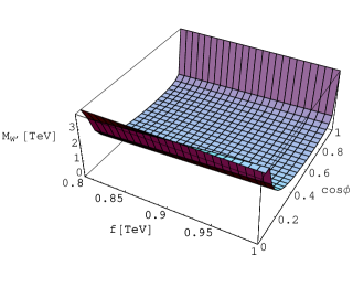
Figure 3: $M_{W^{\prime}}$ as a function of $\cos\psi$ and $f$, with 0.8 TeV $<f<1$ TeV.

Let us discuss now briefly how the heavy gauge boson masses depend on mixing angles $\psi$. We know that $M_{W^{\prime}}$ is of the order of $f\sim$ TeV (see eq.(12)) and from these equations we can obtain restrictions on the mixing angles. In Fig.3 we show the dependence of $M_{W^{\prime}}$ on $\cos\psi$ and the scale $f$. We found that 0.5 $<\cos\psi<$ 0.8 implies masses smaller than 0.6 TeV and then these values for $\cos\psi$ can be ruled out. From this results we get the preferred ranges: $\cos\psi<$ 0.5 or $\cos\psi>$ 0.7.

Taking into account the above bounds on the LH model parameters we now focus on obtaining the corresponding $\mu$ values according to our previous one-loop computation which includes both, the fermionic and gauge bosons contributions. We find that, in the case of the Model II, the lowest allowed value for $\mu$ is $\mu=$0.34 TeV being $\lambda_{T}$=0.7, $f=$0.8 TeV, $\Lambda=$11.95 TeV and $\cos\psi=$0.2. However, as discussed in ATP , it is also needed to add in principle the additional constraint $\mu^{2}=\lambda v^{2}$. Then in Fig.4 we show as an example the allowed regions for the Model II. Two different regions can be found. This is due to the mixing angle coming from the heavy gauge boson mass. In this case the lowest value for $\mu$ is $\mu=$0.491 TeV corresponding to $\lambda_{T}=$0.55, $f=$0.95 TeV, $\Lambda$=10 TeV and $\cos\psi=$0.47. Therefore it is clear that the condition $\mu^{2}=\lambda v^{2}$ is relevant in order to constraint the possible values of the LH model parameters.

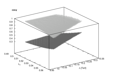
Figure 4: Values of $\lambda_{T}$, $\Lambda$ and $\cos\psi$, with 0.5 $<\lambda_{T}<2$, $10$ TeV $<\Lambda<12$ TeV, $0<\cos\psi<1$, $M_{W^{\prime}}>0.7$ TeV and $f=0.95$ TeV, which satisfy the condition $\mu^{2}=\lambda v^{2}$.

A similar analysis have been done for $f=4$ TeV. The results are shown in Fig.5. The allowed region is smaller in this case. The reason for obtaining just some points of the parameter space allowed by the condition $\mu^{2}=\lambda v^{2}$ is that $\mu^{2}$ has a logarithmical dependence on the energy scale $\Lambda$ and a linear dependence on $f$ coming from the new heavy particle masses, while $\lambda$ depends quadratically on $\Lambda/(4\pi f)$. Therefore, greater values of $\Lambda$ leads to a disadvantageous region for $\mu^{2}=\lambda v^{2}$. In this case the lowest value for $\mu$ is $\mu=$0.916 TeV corresponding to $\lambda_{T}=$0.68, $f=$4 TeV, $\Lambda$=50 TeV and $\cos\psi=$0.086.

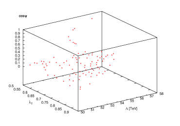
Figure 5: Values of $\lambda_{T}$, $\Lambda$ and $\cos\psi$, with 0.5 $<\lambda_{T}<2$, $0<\cos\psi<1$ and $f=4$ TeV, which satisfy the condition $\mu^{2}=\lambda v^{2}$.

From the above results, it is clear that is difficult to satisfy the condition $\mu^{2}=\lambda v^{2}$ with $\mu$ about $200$ GeV, as expected by the precision electroweak measurements LEP . We also show in Fig.6 the contours of the viable regions in the $\lambda_{T}$-$f$ plane with the condition $\mu^{2}=\lambda v^{2}$. The values of the mixing angle $\psi$ are fixed to the values $\cos\psi=0.1$ (top panel) and $\cos\psi=0.7$ (bottom panel). We check that the results for $\cos\psi$ closed to $1$, i.e $\cos\psi=0.995$, are similar to the ones for $\cos\psi=0.1$. The condition $\Lambda\lesssim 4\pi f$ is imposed. One can see that values of $f$ around $1-3$ TeV are the preferred ones for our selected choices of the LH parameters. However the $\mu$ values are higher than about $350$ GeV for all cases. Therefore, it is clear that it is not enough to consider the one-loop effective potential of the LH model.

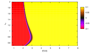
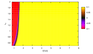
Figure 6: Contours of the viable regions in the $\lambda_{T}$-$f$ plane with the condition $\mu^{2}-\lambda v^{2}=0$. $\cos\psi$ is fixed to $=0.1$ (top panel) and $0.7$ (bottom panel).

VI Conclusions

In this work we have completed the computation of the one-loop effective Higgs potential in the context of two versions (Model I and Model II) of the LH model. In particular we have obtained the values of the radiatively generated $\mu$ and $\lambda$ parameters. Our computation includes the effect of virtual heavy quarks $t,b$ and $T$, together with the heavy and electroweak gauge bosons present in the LH model. We have also clarify the role of the GB when a cutoff is used to regulate the ultraviolet divergencies. These GB do not contribute to the Higgs effective potential at the one-loop level but they do at higher orders. The values of $\mu$ and $\lambda$ that we get have the right signs and are compatible in principle with all the phenomenological constraints set on the LH model parameter space.

However the values found for the $\mu$ parameter are too high to be compatible with the expected Higgs mass, which should not be larger than about 200 GeV according to the electroweak precision data. This problem is even worst if one takes into account the relation $\mu^{2}=\lambda v^{2}$ which must hold on the $\mu$ and $\lambda$ parameters of the effective Higgs potential to reproduce the SM. As a conclusion the low-energy, one-loop effective potential of the LH model cannot reproduce the SM potential with a low enough Higgs mass to agree with the standard expectations. However there are some indications suggesting that higher order GB loops could reduce the Higgs boson mass so that complete compatibility with the experimental constraints can be obtained. Work is in progress in order to check if this is really the case Future .

VII Appendix A

From (10) it is possible to find the gauge bosons couplings to doublet Higgs, needed for our computations, which turn to be:

• Massless gauge bosons-massless gauge bosons:

  $$\frac{g^{2}}{4}(-\frac{1}{3f^{2}}(HH^{{\dagger}})^{2})W_{\mu}^{a}W^{a\mu},\hskip 7.11317pta=1,2,3,$$ (91)

  $$\frac{g^{{}^{\prime}2}}{4}(-\frac{1}{3f^{2}}(HH^{{\dagger}})^{2})B_{\mu}B^{\mu},$$

  $$- \frac{1}{2}gg^{{}^{\prime}}(H^{0*}H^{+}+H^{0}H^{+*})W_{\mu}^{1}B^{\mu},$$ (92)

  $$- \frac{i}{2}gg^{{}^{\prime}}(H^{0*}H^{+}-H^{0}H^{+*})W_{\mu}^{2}B^{\mu},$$ (93)

  $$- \frac{1}{2}gg^{{}^{\prime}}(H^{0}H^{0*}+H^{+}H^{+*})W_{\mu}^{3}B^{\mu}.$$ (94)

• Heavy gauge bosons-massless gauge bosons:

  $$g_{W^{\prime}W}HH^{{\dagger}}W_{\mu}^{{}^{\prime}a}W^{a\mu},\hskip 7.11317pt$$ (96)

  $$g_{B^{\prime}B}HH^{{\dagger}}B_{\mu}^{{}^{\prime}}B^{\mu},$$

  $$- g_{W^{\prime}B}(H^{0*}H^{+}+H^{0}H^{+*})W_{\mu}^{{}^{\prime}1}B^{\mu},$$ (97)

  $$-i g_{W^{\prime}B}(H^{0*}H^{+}-H^{0}H^{+*})W_{\mu}^{{}^{\prime}2}B^{\mu},$$ (98)

  $$- g_{W^{\prime}B}(H^{0}H^{0*}-H^{+}H^{+*})W_{\mu}^{{}^{\prime}3}B^{\mu},$$ (99)

  $$- g_{B^{\prime}W}(H^{0*}H^{+}+H^{0}H^{+*})B^{\prime}_{\mu}W^{\mu 1},$$ (100)

  $$-i g_{B^{\prime}W}(H^{0*}H^{+}-H^{0}H^{+*})B^{\prime}_{\mu}W^{\mu 2},$$ (101)

  $$- g_{B^{\prime}W}(H^{0}H^{0*}-H^{+}H^{+*})B^{\prime}_{\mu}W^{\mu 3}.$$ (102)

• Heavy gauge bosons-heavy gauge bosons:

  $$\left\{g_{W^{\prime}W^{\prime}}\left[3(g_{1}^{2}+g_{2}^{2})^{2}(H^{0*}H^{+}+H^{0}H^{+*})^{2}+4g_{1}^{2}g_{2}^{2}(HH^{{\dagger}})^{2}\right]-\frac{1}{4}g^{2}HH^{{\dagger}}\right\}W_{\mu}^{{}^{\prime}1}W^{{}^{\prime}1\mu},$$ (107)

  $$\left\{g_{W^{\prime}W^{\prime}}\left[-3(g_{1}^{2}+g_{2}^{2})^{2}(H^{0*}H^{+}-H^{0}H^{+*})^{2}+4g_{1}^{2}g_{2}^{2}(HH^{{\dagger}})^{2}\right]-\frac{1}{4}g^{2}HH^{{\dagger}}\right\}W_{\mu}^{{}^{\prime}2}W^{{}^{\prime}2\mu},$$

  $$\left\{g_{W^{\prime}W^{\prime}}\left[-12(g_{1}^{2}+g_{2}^{2})^{2}(H^{0}H^{0*}H^{+}H^{+*})+(10g_{1}^{2}g_{2}^{2}+3(g_{1}^{4}+g_{2}^{4}))(HH^{{\dagger}})^{2}\right]-\frac{1}{4}g^{2}HH^{{\dagger}}\right\}W_{\mu}^{{}^{\prime}3}W^{{}^{\prime}3\mu},$$

  $$\left\{g_{B^{\prime}B^{\prime}}\left[3(g_{1}^{{}^{\prime}4}+g_{2}^{{}^{\prime}4})+10g_{1}^{{}^{\prime}2}g_{2}^{{}^{\prime}2}\right](HH^{{\dagger}})^{2}-\frac{1}{4}g^{{}^{\prime}2}HH^{{\dagger}}\right\}B^{{}^{\prime}}_{\mu}B^{{}^{\prime}\mu},$$

  $$g_{W^{\prime}B^{\prime}}(H^{0*}H^{+}+H^{0}H^{+*})W_{\mu}^{{}^{\prime}1}B^{{}^{\prime}\mu},$$

  $$i g_{W^{\prime}B^{\prime}}(H^{0*}H^{+}-H^{0}H^{+*})W_{\mu}^{{}^{\prime}2}B^{{}^{\prime}\mu},$$ (109)

  $$g_{W^{\prime}B^{\prime}}(H^{0}H^{0*}+H^{+}H^{+*})W_{\mu}^{{}^{\prime}3}B^{{}^{\prime}\mu}.$$

The different couplings appearing above are given by:

$g_{W^{\prime}W^{\prime}}=\frac{1}{48f^{2}(g_{1}^{2}+g_{2}^{2})},$           $g_{B^{\prime}B^{\prime}}=\frac{1}{48f^{2}(g_{1}^{{}^{\prime}2}+g_{2}^{{}^{\prime}2})},$

$g_{W^{\prime}W}=\frac{g(g_{1}^{2}-g_{2}^{2})}{4\sqrt{g_{1}^{2}+g_{2}^{2}}},$               $g_{B^{\prime}B}=\frac{g^{\prime}(g_{1}^{{}^{\prime}2}-g_{2}^{{}^{\prime}2})}{4\sqrt{g_{1}^{{}^{\prime}2}+g_{2}^{{}^{\prime}2}}},$

$g_{W^{\prime}B}=\frac{g^{\prime}(g_{1}^{2}-g_{2}^{2})}{4\sqrt{g_{1}^{2}+g_{2}^{2}}},$               $g_{B^{\prime}W}=\frac{g(g_{1}^{{}^{\prime}2}-g_{2}^{{}^{\prime}2})}{4\sqrt{g_{1}^{{}^{\prime}2}+g_{2}^{{}^{\prime}2}}}.$

$g_{W^{\prime}B^{\prime}}=\frac{g_{1}^{{}^{\prime}2}g_{2}^{2}+g_{1}^{2}g_{2}^{{}^{\prime}2}}{4\sqrt{(g_{1}^{2}+g_{2}^{2})(g_{1}^{{}^{\prime}2}+g_{2}^{{}^{\prime}2})}},$

VIII Appendix B

The integrals appearing in our computations are:

$$I_{0}(M^{2}) \equiv \int d\tilde{p}\frac{i}{p^{2}-M^{2}}$$

$$I_{1}(M^{2}) \equiv \int d\tilde{p}\frac{i}{(p^{2}-M^{2})^{2}}$$

$$I_{2}(M^{2}) \equiv \int d\tilde{p}\frac{i}{p^{2}(p^{2}-M^{2})}$$

$$I_{2}(0) \equiv \int d\tilde{p}\frac{i}{p^{4}}$$

$$I_{3}(M_{a}^{2},M_{b}^{2}) \equiv \int d\tilde{p}\frac{i}{(p^{2}-M_{a}^{2})(p^{2}-M_{b}^{2})}.$$

Using an ultraviolet cutoff $\Lambda$ these integrals are found to be:

$$I_{0}(M^{2}) = \frac{1}{(4\pi)^{2}}\left[\Lambda^{2}-M^{2}\log\left(1+\frac{\Lambda^{2}}{M^{2}}\right)\right]$$

$$I_{1}(M^{2}) = -\frac{1}{(4\pi)^{2}}\left[\log\left(1+\frac{\Lambda^{2}}{M^{2}}\right)-\frac{1}{1+\frac{M^{2}}{\Lambda^{2}}}\right]$$

$$I_{2}(M^{2}) = -\frac{1}{(4\pi)^{2}}\log\left(1+\frac{\Lambda^{2}}{M^{2}}\right)$$

$$I_{2}(0) = -\frac{1}{(4\pi)^{2}}\log\left(\frac{\Lambda^{2}}{m^{2}}\right)$$

$$I_{3}(M_{a}^{2},M_{b}^{2}) = -\frac{1}{(4\pi)^{2}}\frac{1}{M_{a}^{2}-M_{b}^{2}}\left[M_{a}^{2}\log\left(1+\frac{\Lambda^{2}}{M_{a}^{2}}\right)\right.$$

$$- \left.M_{b}^{2}\log\left(1+\frac{\Lambda^{2}}{M_{b}^{2}}\right)\right]$$

where $m$ is an infrared cutoff.

Acknowledgements: This work is supported by DGICYT (Spain) under project number BPA2005-02327. The work of S.P. is supported by the I3P-Contract of CSIC at IFIC - Instituto de Física Corpuscular, Valencia. The work of L. Tabares-Cheluci is supported by FPU grant from the Spanish M.E.C.

References

• (1) H. Georgi and A. Pais, Phys. Rev. D10, 539 (1974) H. Georgi and A. Pais, Phys. Rev. D12, 508 (1975).
• (2) N. Arkani-Hamed, A.G. Cohen, E.Katz, A.E.Nelson, JHEP 0207:034 (2002), hep-ph/0206021.
• (3) M. Schmaltz, D. Tucker-Smith, Ann. Rev. Nucl. Part. Sci.  55 (2005) 229, hep-ph/0502182.
• (4) M. Perelstein, Prog. Part. Nucl. Phys.  58 (2007) 247, hep-ph/0512128.
• (5) T. Han, Heather E. Logan, B. McElrath, Lian-Tao Wang, Phys. Rev. D 67,095005 (2003), hep-ph/0301040.
• (6) F. Bazzocchi, M. Fabbrichesi, M. Piai, Phys. Rev.  D72 (2005) 095019, hep-ph/0506175.
• (7) A. Dobado, L. Tabares, S. Peñaranda, hep-ph/0606031, Published in Eur. Phys. J. C (2007), http://dx.doi.org/10.1140/epjc/s10052-007-0232-8.
• (8) M. Perelstein, M. E. Peskin, A. Pierce, Phys. Rev. D69, 075002 (2004), hep-ph/0310039.
• (9) A. Dobado, A. Gómez-Nicola, A.L. Maroto and J.R. Peláez, Effective Lagrangians for the Standard Model, Springer-Verlag, Heidelberg, (1997).
• (10) J. Zinn-Justin,Quantum Field Theory and Critical Phenomena, Oxford University Press, New York, 1989; A. Dobado and J. R. Peláez, Phys. Lett. B286, 136 (1992); A. Dobado, A. López and J. Morales, Il Nuovo Cimento (Nuclei, particles and fields) 108A, 335 (1995); D. Espriu and J. Matias Nucl. Phys. B418 (1994) 494.
• (11) C. Csaki, J. Hubisz, G. D. Kribs, P. Meade, J. Terning, Phys. Rev. D67 (2003) 115002, hep-ph/0211124.
• (12) C. Csaki, J. Hubisz, G. D. Kribs, P. Meade, J. Terning, Phys. Rev. D68, 035009 (2003), hep-ph/0303236.
• (13) Z. Han, W. Skiba, Phys. Rev.  D72, 035005 (2005), hep-ph/0506206; H.E. Logan, Phys. Rev. D70, 115003 (2004), hep-ph/0405072; T. Han, H. E. Logan, B. McElrath, L. T. Wang, Phys. Lett.  B563, 191 (2003) [Erratum-ibid. B603, 257 (2004)], hep-ph/0302188.
• (14) J. L. Hewett, F. J. Petriello, T. G. Rizzo, JHEP 0310, 062 (2003), hep-ph/0211218. T. Gregoire, D. R. Smith, J. G. Wacker, Phys. Rev.  D69, 115008 (2004), hep-ph/0305275; M. C. Chen and S. Dawson, Phys. Rev. D70, 015003 (2004), hep-ph/0311032; W. Kilian, J. Reuter, Phys. Rev. D70, 015004 (2004), hep-ph/0311095; G. Marandella, C. Schappacher, A. Strumia, Phys. Rev. D72, 035014 (2005), hep-ph/0502096.
• (15) M.C. Chen, Mod. Phys. Lett.  A21, 621 (2006), hep-ph/0601126; S.R. Choudhury, A.S. Cornell, N. Gaur, A. Goyal, hep-ph/0604162; J.A. Conley, J. Hewett, M. P. Le, Phys. Rev. D72, 115014 (2005), hep-ph/0507198; C.O. Dib, R. Rosenfeld, A. Zerwekh, AIP Conf. Proc.  815, 296 (2006), hep-ph/0509013; Z. Berezhiani, P.H. Chankowski, A. Falkowski, S. Pokorski, Phys. Rev. Lett.  96, 031801 (2006), hep-ph/0509311.
• (16) A. Manohar, H. Georgi, Nucl. Phys. B234, 189 (1984); M. A. Luty, Phys. Rev. D57, 1531 (1998), hep-ph/9706235; A. G. Cohen, D. B. Kaplan, A. E. Nelson, Phys. Lett. B412, 301 (1997), hep-ph/9706275; J. Alberto Casas, Jose Ramón Espinosa, Irene Hidalgo, JHEP 0503:038.
• (17) http://lepewwg.web.cern.ch/LEPEWWG
• (18) A. Dobado, L. Tabares-Cheluci, S. Peñaranda; in progress.