Method for comparing finite temperature field theory results with lattice data

Abstract

The values of the presently available truncated perturbative expressions for the pressure of the quark-gluon plasma at finite temperatures and finite chemical potential are trustworthy only at very large energies. When used down to temperatures close to the critical one $(T_{c})$, they suffer from large uncertainties due to the renormalization scale freedom. In order to reduce these uncertainties, we perform resummations of the pressure by applying two specific Padé-related approximants to the available perturbation series for the short-distance and for the long-distance contributions. In the two contributions, we use two different renormalization scales which reflect different energy regions contributing to the different parts. Application of the obtained expressions at low temperatures is made possible by replacing the usual four-loop ${\overline{\rm MS}}$ beta function for $\alpha_{s}$ by its Borel-Padé resummation, eliminating thus the unphysical Landau singularities of $\alpha_{s}$. The obtained results are remarkably insensitive to the chosen renormalization scale and can be compared with lattice results – for the pressure $p$, the chemical potential contribution $\Delta p$ to the pressure, and various susceptibilities. A good qualitative agreement with the lattice results is revealed down to temperatures close to $T_{c}$.

I Introduction

The behavior of QCD matter at nonvanishing temperature and (quark or hadron) densities can be approached theoretically from two sides, both technically and kinematically. On the one hand, QCD-lattice calculations allow an analysis of the kinematic region of rather low temperatures $T$ (around but above the phase-transition temperature $T_{c}$, presently $T\lesssim 5T_{c}$) and even lower values of the chemical potentials $\mu_{f}$ ($f$ denotes the different quark flavors). The latter restriction is due to the fact that nonzero values of the chemical potential $\mu$ render the weight function in the partition function complex thus not permitting direct application of the standard Monte Carlo techniques. There are several tricks to circumvent this “sign-problem”: reweighting Fodor , Taylor expansion around $\mu=0$ Allton , analytic continuation from imaginary $\mu$ values Forcrand , canonical formalism Krat . All of them are trustworthy only for small $\mu$ values. On the other hand, the behavior at high $T$ and $\mu<2\pi T$ is expected to be described reliably by finite temperature (and density) perturbation theory (FTPT). Significant progress has been made within this latter approach during the last twenty years and the calculation of the thermodynamic potential (free energy or, equivalently, the pressure function $p$) has recently been pushed forward to the four-loop level, both for $\mu=0$ KLRS1 and for finite chemical potential Vuo . This is a big achievement because the corresponding truncated perturbation series (TPS) is in powers of the QCD-strong coupling parameter $g$ rather than $a\equiv g^{2}/(4\pi^{2})\equiv\alpha_{s}/\pi$, due to the well-known necessity of removing finite temperature infrared (IR) divergences by resumming the essential IR-sensitive diagrams (“daisy diagrams”) to all orders. The final series is up to 6th order in $g$, and that is essentially all that could be expected from perturbation theory since terms proportional to $g^{6}$ (not $g^{6}~{}\ln~{}g$) and higher include genuine non-perturbative contributions which could be accessed only by non-perturbative methods, e.g. lattice calculations.

Of course, any perturbatively obtained result is expected to represent the true physical situation only when the coupling parameter is small enough, which is the case in QCD at sufficiently high temperatures. Nevertheless, evaluations of the 6th order result (for $p$ and for $\Delta p=p(\mu)-p(0)$) down to temperatures below 1 GeV have been made in the literature, and the results could be brought in accordance with non-perturbative lattice data (available for $T$ up to $1$ GeV). At first sight this could be considered a triumph of finite temperature perturbation theory, and might tentatively be attributed to the higher order available. A second and more careful glimpse, however, reveals several sobering observations. The first problem is that the convergence behavior of the truncated perturbation series is manifestly weak: if increasingly higher orders in the series are added, the corresponding partial sums are changing wildly, jumping up and down. Only the step from 5th to 6th order has signs of moderation, but it is by no means clear whether this happens by chance or indicates a systematic improvement of the situation. Further, a common relatively high renormalization scale (RScl) $\nu\approx 2\pi T$ ($\gg T$) is used in such evaluations. For comparison with independent lattice data, the TPS results are used down to small $T$ values where the lattice results are available. But here, another problem occurs: in each available order the corresponding TPS shows a dependence of the chosen RScl $\nu$, which is particularly strong for lower temperatures, thus making a consistent comparison of perturbative results (when used at such low energies) with lattice data doubtful. In fact we have no clear physical motivation for the best choice of $\nu$. In general, $\nu$ should be chosen such that large (momentum dependent) logarithms in the TPS coefficients are avoided, which means – within an asymptotically free theory like QCD – that one is always on the safe side if $\nu$ is taken to be near the lowest energy scales involved in the considered quantity. For the quark-gluon plasma at (high) temperature $T$ (and for given chemical potentials $\mu_{f}$), what is the appropriate energy scale? Usually in the literature, the energy $2\pi T$ of the lowest nonzero mode is taken as a measure since it determines the average energy of the constituents. But due to the collective effects additional (lower) physical scales are generated, namely the electric and magnetic screening masses (being of order $gT$ and $g^{2}T$, respectively). So what to choose for $\nu$? This question is not a purely theoretical one, but of considerable practical importance, because of the mentioned strong dependence of the TPS on $\nu$. And even if we neglect this intertwining of different scales within the thermodynamic quantities, and stick to $2\pi T$ as the relevant scale, we observe that a change of $\nu$ by a single factor of 2 implies such a wide variation of the perturbative results at $T\sim T_{c}$ that no firm conclusion can be drawn as to the matching with lattice data (cf. Figs. 6 and 7). It is clear, therefore, that no successful matching procedure can be obtained unless the strong RScl dependence is pinched down by improving the perturbative results.

Within the present paper we offer a way for avoiding this unwanted (and unphysical) ambiguity by applying perturbation-theory-improving resummations of the basic TPS’s. In this way we obtain what we consider a more reliable, but still perturbation-theory-based, description of the interesting thermodynamic quantities (here the pressure $p$) which, among other things, allow for a more credible comparison with lattice results. The method rests on replacing the (partially resummed) TPS by approximants which are much more stable under the variation of $\nu$ than the TPS’s themselves. It is well known that specifically Padé approximants Padebook for physical (measurable) quantities are stable under $\nu$ variation Gardi , whereas similar improved Baker-Gammel approximants show this stability exactly Cvetic . In a recent work GRp we have utilized Padé-related approximants to produce RScl-stable expressions for the pressure of the quark-gluon plasma at finite (large) temperature and zero chemical potential. Here, we apply the same technique to the case of finite nonzero quark chemical potential. In both cases, the gratifying fact is the high order of the available TPS which allows the use of higher-order Padé-related approximants and the choice of the most appropriate ones (see later).

From the technical point of view we encounter a specific problem when applying Padé-related approximants directly to finite temperature perturbation theory. This is due to the fact that two different (infinite) classes of diagrams get involved in the whole mechanism: on the one hand those whose resummation is necessary for taming the finite-temperature IR divergences and which lead to contributions in powers of $g$ (the so-called “daisy diagrams”); on the other hand the other diagrams, which give contributions in powers of $g^{2}$ and whose conversion from the TPS (polynomials) into Padé approximants (rational functions) had been known to result in RScl stability (which is exact in the large-$\beta_{0}$ limit in the case of the diagonal Padé approximants Gardi ). Therefore, care has to be taken to avoid double counting when performing both resummations. As we have shown in Refs. GRp , a safe method consists in first decomposing the pressure into two parts, one containing the low-energy (effectively zero) modes and being responsible for the long-distance behavior of the correlation functions, and the other stemming from the nonzero modes and determining the short-range physics. Since both regions are, in principle, separately accessible by experiments, the corresponding expressions are physical in the sense that they should be independent of the renormalization scale $\nu$ (at least up to the specified order in $g$). Further, no (infinite) resummation enters into the perturbation expressions of those parts when dimensional reduction is applied Gross . Therefore, one can safely apply Padé-related resummation to both parts independently and thus obtain two expressions which are both almost independent of the RScl choice. When using them down to low energies $(T\sim T_{c})$, we face another problem: the coupling parameter $a(Q^{2})$ acquires unphysical (Landau)singularities at low energies $Q\lesssim 1$ GeV if using ${\overline{\rm MS}}$ TPS $\beta$ function. We circumvent this problem by using again appropriately resummed versions of $\beta$. We finally end up with expressions for the pressure and for other measurable quantities (quark number susceptibilities) which are almost free of the RScl uncertainty and therefore apt for comparison with lattice data.

In Sec. II we present the perturbative results on which our analysis rests and describe how to perform the physical separation of the pressure into the long-range and the short-range part. Section III contains an analysis of the possible resummation procedures which leads to the optimal choice. We then present the numerical results, where we put the main emphasis both on the effect of finite $\mu$ values and on the comparison with the corresponding lattice data. Appendix A compiles basic formulae and expressions, available in the literature and adapted to our approach, including expressions for the coefficients of the TPS’s. Appendix B describes the method which allows us to extrapolate the QCD renormalization group equation to sufficiently low energies, thereby circumventing the unphysical Landau singularities of the coupling parameter.

II Separation of Long- and Short-Distance Pressure

Our starting point are the FTPT results for the pressure of the quark-gluon plasma which, for a homogeneous system, is equal to the free energy per volume (up to a sign difference) – considered as a function of its temperature $T$ and the chemical potentials of the various quark flavors $\mu_{f}~{}(f=1,...n)$. It has been calculated up to ${\cal O}(g^{6}\ln g)$ by K. Kajantie et al. KLRS1 for the case of vanishing chemical potentials, and for the general case $(\mu_{f}\not=0)$ by A. Vuorinen Vuo . These high order results include the summation of an infinite class of certain diagrams – necessary for taming an IR singularity which occurs only at $T\not=0$. The final results could be practically achieved only by a technical trick, namely by separating the energy-momentum region of the contributing modes into three parts, characterized by the momentum scales $2\pi T,~{}~{}gT$ and $g^{2}T$, such that the full pressure $p$ is decomposed according to

$$p=p_{\rm E}+p_{\rm M}+p_{\rm G}\ .$$ (1)

Note that this decomposition makes strict sense only for high enough temperatures where $g(T)\lesssim 1$. Here, $p_{\rm E}$ represents the contributions of all degrees of freedom associated with the nonvanishing Matsubara modes, whereas $p_{\rm M}+p_{\rm G}$ comprises the contributions of the zero modes (of bosonic fields), thereby implicitly representing also the necessary sum over all (daisy) diagrams. The latter ones are static modes, hence their contributions can be effectively described by a three-dimensional (in general $d$-dimensional) purely bosonic field theory (dimensional reduction Gross ) determined by the electrostatic QCD (EQCD) Lagrangian

$${\cal L}_{\rm EQCD}=\frac{1}{2}{\rm Tr}\tilde{F}^{2}_{ij}+{\rm Tr}[D_{i},\tilde{A}_{0}]^{2}+m_{\rm E}^{2}{\rm Tr}\tilde{A}^{2}_{0}+\lambda^{(1)}_{\rm E}({\rm Tr}\tilde{A}^{2}_{0})^{2}+\lambda^{(2)}_{\rm E}{\rm Tr}\tilde{A}_{0}^{4}+i\frac{g^{3}}{3\pi^{2}}\left(\sum_{f}\mu_{f}\right){\rm Tr}\tilde{A}^{3}_{0}+...$$ (2)

Here $\tilde{A}_{0}$ denotes an effective ($d$-dimensional) scalar field and the $\tilde{A}_{i}~{}(i=1,...d)$ define a $d$-dimensional vector field, both in matrix notation $(\tilde{A}_{\mu}\equiv\tilde{A}_{\mu}^{a}T^{a})$; $D_{i}=\partial_{i}-ig_{\rm E}\tilde{A}_{i}$; $\tilde{F}_{ij}=(i/g_{\rm E})[D_{i},D_{j}]$. The parameters of this effective theory are the (electrostatic) screening mass $m_{\rm E}~{}(\sim gT)$, the effective coupling parameter $g_{\rm E}^{2}~{}(\sim g^{2}T)$ and the four-vertex couplings $\lambda^{(1)}_{\rm E},\lambda^{(2)}_{\rm E}(\sim g^{4}T)$. In the case of $d=3,~{}~{}\lambda^{(1)}_{\rm E}$ and $\lambda^{(2)}_{\rm E}$ are not independent and one can choose $\lambda^{(2)}_{\rm E}=0$ – this will be done in the following. There are additional coupling parameters connected with Lagrangian operators of higher dimensions, since ${\cal L}_{\rm EQCD}$ defines a non-renormalizable theory which makes sense only for momenta below a certain (UV)cutoff $\Lambda_{\rm E}$. In our case $\Lambda_{\rm E}$ separates the region of momenta $\sim 2\pi T$ from the momenta $\sim gT$ and smaller.

The effective parameters can be connected to the parameters of the underlying QCD by means of the well-known matching procedure Braaten:1996ju yielding

$$m_{\rm E}^{2} = T^{2}{\Bigg{\{}}g^{2}\left[A_{4}+\epsilon\left(A_{5}^{(\nu)}\ln\frac{\nu_{c}}{2\pi T}+A_{5}\right)+{\cal O}(\epsilon^{2})\right]$$ (3)

$$+\frac{1}{(4\pi)^{2}}g^{4}\left[A_{6}^{(\nu)}\ln\frac{\nu_{c}}{2\pi T}+A_{6}+{\cal O}(\epsilon)\right]+{\cal O}(g^{6}){\Bigg{\}}}\ ,$$

$$g_{\rm E}^{2} = T{\Bigg{\{}}g^{2}+\frac{1}{(4\pi)^{2}}g^{4}\left[A^{(\nu)}_{7}\ln\frac{\nu_{c}}{2\pi T}+A_{7}+{\cal O}(\epsilon)\right]+{\cal O}(g^{6}){\Bigg{\}}}\ ,$$ (4)

$$\lambda^{(1)}_{\rm E} = T{\Bigg{\{}}\frac{1}{(4\pi)^{2}}g^{4}\left[\beta_{\rm E4}+{\cal O}(\epsilon)\right]+{\cal O}(g^{6}){\Bigg{\}}},\qquad\lambda_{\rm E}^{(2)}=0\ .$$ (5)

Here, $\epsilon=(3-d)/2$; coefficients $A_{4}$-$A_{7}$, $A_{5}^{(\nu)}$-$A_{7}^{(\nu)}$ and $\beta_{\rm E4}$ are complicated functions of the chemical potentials, the latter appearing in the coefficients via the dimensionless quantities ${\overline{\mu}_{f}}\equiv\mu_{f}/(2\pi T)$. Their expressions are collected in Appendix A, together with other coefficients to appear in Eqs. (8)-(10). Note that the common RScl $\nu_{c}$ appears in these expressions. The effective mass $m_{\rm E}\sim gT$ arises due to the color-electric screening.

Since there is, in addition, color-magnetic screening at energies proportional to the corresponding magnetic screening mass $m_{\rm M}\sim g^{2}T$, the long-distance part of the pressure can be further subdivided into $p_{\rm M}$ and $p_{\rm G}$, where $p_{\rm M}$ is determined by ${\cal L}_{\rm EQCD}$ and $p_{\rm G}$ by the (magnetostatic) Lagrangian

$${\cal L}_{\rm MQCD}=\frac{1}{2}{\rm Tr}\tilde{F}_{ij}+...$$ (6)

with $\tilde{F}_{ij}=(i/g_{\rm M})[\tilde{D}_{i},\tilde{D}_{j}]$ and $\tilde{D}_{i}=\partial_{i}-ig_{\rm M}\tilde{A}_{i}$. This Lagrangian defines the effective theory for energies below $\Lambda_{\rm M}$, i.e., for energies $\sim g^{2}T$ and smaller. A similar matching procedure as before determines $g_{\rm M}$ in terms of the parameters of the higher-energy Lagrangian ${\cal L}_{\rm EQCD}$ and gives

$$g^{2}_{\rm M}=g_{\rm E}^{2}+{\cal O}(g^{3}).$$ (7)

In the case of nonzero chemical potentials, two scales get involved ($T$ and $\mu\equiv\mu_{f}$) and, therefore, the concept of dimensional reduction is expected to be applicable only if the magnitude of the chemical potentials is small compared to $2\pi T$ HLP . From comparison with numerical results for correlation lengths, it is expected that the restriction $\mu\leq 4T$ is safe.

Based on Lagrangians (2) and (6), and on the ordinary QCD-Lagrangian, the various parts of the pressure have been calculated perturbatively by Vuorinen Vuo . The calculations are based on dimensional regularization with a common RScl $\nu_{c}$ (the notation $\bar{\Lambda}$ is used in Ref. Vuo for the common RScl).

The result for $p_{\rm E}$ is

$$\frac{p_{\rm E}}{T} =T^{3} {\Bigg{[}}A_{1}+g^{2}\left(A_{2}+{\cal O}(\epsilon)\right)$$ (8)

$$+\frac{1}{(4\pi)^{2}}g^{4}\left(\frac{1}{\epsilon}6A_{4}+A_{3}^{(\nu)}\ln\frac{\nu_{c}}{2\pi T}+A_{3}+{\cal O}(\epsilon)\right)$$

$$+\frac{1}{(4\pi)^{4}}g^{6}\left(\beta_{\rm E1}+{\cal O}(\epsilon)\right)+{\cal O}(g^{8}){\Bigg{]}}\ .$$

Coefficients $A_{i}~{}(i=1,2,3)$ and $A_{3}^{(\nu)}$ are collected in Appendix A. Coefficient $\beta_{\rm E1}$ at $g^{6}$ is still unknown. However, $\beta_{\rm E1}$ must include a term proportional to $1/\epsilon$. The $1/\epsilon$-terms will be disposed of in the following because such terms must cancel in the sum (1), and the finite part of $\beta_{\rm E1}$ will contain a free (adjustable) parameter later in this work.

The results for $p_{\rm M}$ and $p_{\rm G}$, which can be obtained from the effective Lagrangians (2) and (6), respectively, are Vuo

$$\frac{p_{\rm M}}{T} = m_{\rm E}^{3}\frac{2}{3\pi}\left\{1+\frac{1}{4\pi}3^{2}\frac{g_{\rm E}^{2}}{m_{\rm E}}\left[-\frac{3}{4}-\ln\frac{\nu_{c}}{2m_{\rm E}}\right]\right.$$ (9)

$$+ \frac{1}{(4\pi)^{2}}3^{3}\left(\frac{g_{\rm E}^{2}}{m_{\rm E}}\right)^{2}\left[-\frac{89}{24}-\frac{\pi^{2}}{6}+\frac{11}{6}\ln 2\right]$$

$$+ \frac{1}{(4\pi)^{3}}3^{4}\left(\frac{g_{\rm E}^{2}}{m_{\rm E}}\right)^{3}\left[\alpha_{\rm M1}8\ln\frac{\nu_{c}}{2m_{\rm E}}+\beta_{\rm M1}+\frac{5}{81}(\sum_{f}{\overline{\mu}_{f}})^{2}\left(\alpha_{\rm M2}\ln\frac{\nu_{c}}{2m_{\rm E}}+\frac{1}{4}\beta_{\rm M2}\right)\right]$$

$$- \left.\frac{15}{8\pi}\frac{\lambda_{\rm E}^{(1)}}{m_{\rm E}}\right\}+$$

$$+ \frac{1}{\epsilon}m_{\rm E}^{3}\frac{2}{3\pi}\left\{\frac{1}{4\pi}3^{2}\frac{g_{\rm E}^{2}}{m_{\rm E}}\left(-\frac{1}{4}\right)+\frac{1}{(4\pi)^{3}}3^{4}\left(\frac{g_{\rm E}^{2}}{m_{\rm E}}\right)^{3}\left[\alpha_{\rm M1}+\frac{5}{81}\alpha_{\rm M2}\frac{1}{4}(\sum_{f}{\overline{\mu}_{f}})^{2}\right]\right\}$$

$$+ {\cal O}(\epsilon)+{\cal O}(g_{\rm E}^{8}/m_{\rm E})\ ,$$

$$\frac{p_{\rm G}}{T} = \frac{2}{3\pi}\frac{1}{(4\pi)^{3}}3^{4}\left(g^{2}_{\rm M}\right)^{3}\left[\alpha_{\rm G}8\ln\frac{\nu_{c}}{2m_{\rm M}}+\delta_{\rm G}+{\cal O}(\epsilon)\right]+\hskip 156.49014pt$$ (10)

$$+ \frac{1}{\epsilon}\frac{2}{3\pi}\frac{1}{(4\pi)^{3}}3^{4}\left(g^{2}_{\rm M}\right)^{3}\alpha_{\rm G}\ .$$

Here, $m_{\rm M}$ is the magnetic screening mass $m_{\rm M}=3g_{\rm M}^{2}$ ($\sim g^{2}T$), and the notation ${\overline{\mu}_{f}}\equiv\mu_{f}/(2\pi T)$ is used. We observe that the chemical potentials show up both explicitly via ${\overline{\mu}_{f}}$ and implicitly via $g_{\rm E}$ and $m_{\rm E}$. Coefficients $\alpha_{\rm M1},\alpha_{\rm M2},\alpha_{\rm G},\beta_{\rm M1},\beta_{\rm M2}$ are independent of $\mu_{f}$ (see Appendix A), and only $\beta_{\rm M2}$ is not yet known. In Eqs. (9) and (10) we have already separated all “divergent” terms (proportional to $1/\epsilon$) from the finite contributions. The quantity $p_{\rm M}/T$ starts effectively with order $g^{3}$ and $p_{\rm G}/T$ with order $g^{6}$. The full $\sim g^{6}$ term in $p_{\rm G}/T$ cannot be determined in a perturbative way; however, $\delta_{\rm G}$ was estimated in Ref. DiRenzo:2006nh to be $\delta_{\rm G}=-0.2\pm 0.6$. Here, it will be treated as a free parameter within the limits $\delta_{\rm G}=0\pm 1$. On the left-hand sides of Eqs. (8)-(10), the common denominator $T$ must in fact be replaced by $T\nu_{c}^{-2\epsilon}$; however, the common factor $\nu_{c}^{-2\epsilon}$ reduces to unity in the $\epsilon\to 0$ limit, and will be ignored because the sum $p_{\rm E}+p_{\rm G}+p_{\rm M}$ is finite in this limit.

Our main task now consists in deducing from these formulae expressions for the physical short-range and long-range parts of the pressure. Thereby the word “physical” indicates that they lead to measurable effects (for instance, the long and/or short-range behavior of static correlation functions, etc.). We proceed in several steps (see also Ref. GRp ):

• Regularization: The long-range part of the pressure is represented by $p_{\rm M}+p_{\rm G}\equiv p_{\rm M+G}$ (both are due to zero mode contributions). We regularize $p_{\rm M+G}$ by adding to $p_{\rm M+G}/T$ the following counterterm:

  $$CT=\frac{1}{\epsilon}6\left\{\frac{1}{(4\pi)^{2}}g_{\rm E}^{2}m_{\rm E}^{2}-36\frac{1}{(4\pi)^{4}}\left[g^{6}_{\rm E}\left(\alpha_{\rm M1}+\alpha_{\rm M2}\frac{5}{324}(\sum_{f}{\overline{\mu}_{f}})^{2}\right)+g^{6}_{\rm M}\alpha_{\rm G}\right]\right\}.$$ (11)

  The same counterterm has to be subtracted from $p_{\rm E}/T$. By expanding the effective-theory-parameters $g_{\rm E}$ and $m_{\rm E}$ in powers of $g$ [cf. Eqs. (3), (4)], one can explicitly show that in this way the $1/\epsilon$-term of order $g^{4}$ in expression (8) for $p_{\rm E}/T$ gets cancelled. Further, the $1/\epsilon$-term of order $g^{6}$ included in the otherwise unknown $\beta_{\rm E1}$ coefficient must also get cancelled when counterterm (11) is subtracted from $p_{\rm E}/T$ of Eq. (8). Counterterm (11) contains one finite term of ${\cal O}(g^{4})$ stemming from $(1/\epsilon)g_{\rm E}^{2}m_{\rm E}^{2}$ since $m_{\rm E}^{2}$ includes a term proportional to $g^{2}\epsilon$, Eq. (3). This finite term then shows up in the new subtracted expression for $p_{\rm E}/T$. In addition, counterterm (11) contains several finite terms of ${\cal O}(g^{6})$ which show up in the new subtracted expression for $p_{\rm E}/T$. Finally, the limit $\epsilon\to 0$ can be performed, yielding finite results both for $p_{\rm E}$ and for $p_{\rm M+G}$.

• Reconstruction of the factorization scale and introduction of various RScl’s: We have already noted that a common renormalization scale (denoted here as $\nu_{c}$) has been used for the perturbative calculations leading to Eqs. (8)-(10). On the other hand, when constructing the physical long- and short-range contributions, respectively, we decompose the whole energy range in the way addressed before, namely

  $${\cal O}(g^{2}T)<\Lambda_{\rm M}<{\cal O}(gT)<\Lambda_{\rm E}<{\cal O}(2\pi T)\ .$$ (12)

  Therefore, these factorization scales $\Lambda_{\rm E}$ and $\Lambda_{\rm M}$ which separate the different energy regions have to emerge in the physical expressions – but only in such a way that, when adding all three contributions they completely disappear. We bring the $\Lambda_{\rm E}$ factorization scale to light in the following way: the scale $\nu_{c}$ in expressions (8)-(10), where $p_{\rm E}/T$ and $p_{\rm M+G}/T$ are modified in the afore-mentioned way by the counterterm (11), is interpreted simultaneously as the factorization scale $\Lambda_{\rm E}$ and as the common RScl $\nu_{c}$. We then evolve $g(\nu=\Lambda_{\rm E})$ in $p_{\rm E}$ to $g(\nu_{\rm E})$ where $\nu=\nu_{\rm E}$ is a new, physically more adequate higher RScl: $\nu_{\rm E}\sim 2\pi T$. On the other hand, in $p_{\rm M+G}$, we evolve $g(\nu=\Lambda_{\rm E})$, which appears implicitly there (explicitly in the RScl-independent $g_{\rm E},m_{\rm E},\lambda_{\rm E}^{(1)}$), to $g(\nu_{\rm M})$ where $\nu=\nu_{\rm M}$ is a new, physically more adequate lower RScl: $\nu_{\rm M}\sim m_{\rm E}$ ($\sim gT$). The evolution is performed according to perturbative renormalization group equation (RGE), requiring RScl independence of $p_{\rm E}$, on the one hand, and of $g_{\rm E}^{2}$ and $m_{\rm E}^{2}$ (and thus of $p_{\rm M+G}$), on the other hand, since all these quantities are physical. In $p_{\rm E}$ this results in $\ln\nu_{\rm E}$-dependent terms in the coefficients of TPS, and in $g_{\rm E}^{2}$ and $m_{\rm E}^{2}$ (which enter $p_{\rm M+G}$) this results in $\ln\nu_{\rm M}$-dependent terms in the coefficients of their TPS’s. The coefficients of expansion of $p_{\rm E}$ in powers of $g^{2}(\nu_{\rm E})$ then have explicitly the “genuinely” $\Lambda_{\rm E}$-dependent parts, and RScl-dependent parts. The coefficients of expansion of $p_{\rm M+G}$ in powers of $(g_{\rm E}^{2}/m_{\rm E})$ remain unchanged, with $\Lambda_{\rm E}$ dependence as before, while the coefficients of expansion of $m_{\rm E}^{2}$ and $g_{\rm E}^{2}$ in powers of $g^{2}(\nu_{\rm M})$ obtain RScl dependence and, at the order considered, lose $\Lambda_{\rm E}$ dependence. Formally, the two RScl’s $\nu_{\rm E}$ and $\nu_{\rm M}$ can take on arbitrary values in these expressions.

• Determination of the $\Lambda_{\rm E}$-dependent part of coefficient at ${\cal O}(g^{6})$ in $p_{\rm E}$: The sum $p_{\rm E}+p_{\rm M+G}$ has to be independent of the factorization scale $\Lambda_{\rm E}$. It can be checked explicitly that this independence is true up to ${\cal O}(g^{4})$. Although the coefficient at $g^{6}$ in $p_{\rm E}$ is not known, its $\Lambda_{\rm E}$ dependence is dictated by the condition of $\Lambda_{\rm E}$ independence of $p_{\rm E}+p_{\rm M+G}$ at ${\cal O}(g^{6})$, when the latter quantity is expanded in powers of a common $g=g(\nu)$. Note that $\Lambda_{\rm E}$ dependence of $p_{\rm M+G}$ at ${\cal O}(g^{6})$ is known, cf. Eqs. (9)-(10). Further, $\nu$ dependence of the coefficient at $g^{6}$ in $p_{\rm E}$ is known from the requirement of the RScl independence of $p_{\rm E}$. The remaining unknown part of the coefficient at ${\cal O}(g^{6})$ in $p_{\rm E}$ (we will call it $\delta_{\rm E}$) is then independent of $\Lambda_{\rm E}$ and of $\nu$, and can again be freely adjusted.

Performing these steps we finally obtain the following form of the physical decomposition of the pressure function into short- and long-distance parts (we denote these physical parts by a bar)

$$p={\bar{p}}_{\rm E}+{\bar{p}}_{\rm M+G}.$$ (13)

The long-distance part, representing the contributions of momenta below the factorization scale $\Lambda_{\rm E}$ (when $gT<\Lambda_{\rm E}<2\pi T$) takes the form

$$\frac{1}{T}{\bar{p}}_{\rm M+G} = \frac{2}{3\pi}m_{\rm E}^{3}\left\{1+\frac{1}{4\pi}3^{2}\left(\frac{g_{\rm E}^{2}}{m_{\rm E}}\right)\left[-\frac{3}{4}-\ln\frac{\Lambda_{\rm E}}{2m_{\rm E}}\right]\right.$$ (14)

$$+ \frac{1}{(4\pi)^{2}}3^{3}\left(\frac{g_{\rm E}^{2}}{m_{\rm E}}\right)^{2}\left[-\frac{89}{24}-\frac{\pi^{2}}{6}+\frac{11}{6}\ln 2\right]$$

$$+ \frac{1}{(4\pi)^{3}}3^{4}\left(\frac{g_{\rm E}^{2}}{m_{\rm E}}\right)^{3}\left[8\alpha_{\rm M1}\ln\frac{\Lambda_{\rm E}}{2m_{\rm E}}+8\alpha_{\rm G}\ln\frac{\Lambda_{\rm E}}{6g_{\rm E}^{2}}+\right.$$

$$+ \left.\beta_{\rm M1}+\delta_{\rm G}-\frac{20}{3^{5}}n^{2}_{f}{\widetilde{\mu}}_{1}^{2}\left(\ln\frac{\Lambda_{\rm E}}{2m_{\rm E}}-\frac{3}{16}\beta_{\rm M2}\right)\right]$$

$$\left.-\frac{15}{8\pi}\frac{\lambda_{\rm E}^{(1)}}{m_{\rm E}}\right\}\ ,$$

where we used notation (35)-(36) for the chemical potential parameter ${\widetilde{\mu}}_{1}$. The parameters $m_{\rm E},g_{\rm E}$ and $\lambda_{\rm E}^{(1)}$ of the effective theory EQCD are defined by their expansion into powers of $g(\nu)\equiv g$

$$m_{\rm E}^{2} = T^{2}A_{4}g^{2}\left\{1+\left(\frac{g}{2\pi}\right)^{2}\left[2\beta_{0}\ln\left(\frac{{\nu}}{2\pi T}\right)+\frac{1}{4}\frac{A_{6}}{A_{4}}\right]+{\cal O}\left(\left(\frac{g}{2\pi}\right)^{4}\right)\right\}$$ (15)

$$g_{\rm E}^{2} = Tg^{2}\left\{1+\left(\frac{g}{2\pi}\right)^{2}\left[2\beta_{0}\ln\left(\frac{{\nu}}{2\pi T}\right)+\frac{1}{4}A_{7}\right]+{\cal O}\left(\left(\frac{g}{2\pi}\right)^{4}\right)\right\}$$ (16)

$$\lambda_{\rm E}^{(1)} = Tg^{4}\;\frac{2}{3}\frac{1}{(4\pi)^{2}}(9-n_{f})\left\{1+{\cal O}\left(\left(\frac{g}{2\pi}\right)^{2}\right)\right\}.$$ (17)

Here, $\beta_{0}=(1/4)(11-2n_{f}/3)$ is the one-loop QCD RGE coefficient, $n_{f}$ being the number of active quark flavors. The RScl $\nu$ in Eqs. (15)-(17) will be $\nu=\nu_{\rm M}$ ($\sim m_{\rm E}\sim gT$), and we fix it according to relation (27). Note that, by the afore-described procedure, the expansion coefficients of $m_{\rm E}^{2}$ and $g_{\rm E}^{2}$ at the considered order do not have any dependence of the factorization scale $\Lambda_{\rm E}$, but are RScl-dependent. The last term in expansion (14) involves the third EQCD matching parameter $\lambda^{(1)}_{\rm E}$ Nadkarni:1988fh ; Landsman:1989be , which is independent of the chemical potentials $\mu_{f}$. This term can be expressed as a power series in powers of $g$, but only the leading term is known $\lambda^{(1)}_{\rm E}/m_{\rm E}\propto g^{3}$. We prefer to express it in powers of the EQCD parameter $g_{\rm E}^{2}/m_{\rm E}$ (Ref. GRp )

$$\lambda^{(1)}_{\rm E}=\frac{2}{3}\frac{1}{(4\pi)^{2}}(9-n_{f})A_{4}\;m_{\rm E}\left(\frac{g_{\rm E}^{2}}{m_{\rm E}}\right)^{3}\left[1+{\cal O}\left(\left(\frac{g_{\rm E}^{2}}{m_{\rm E}}\right)^{2}\right)\right]\ .$$ (18)

While coefficients $\alpha_{\rm M1},\alpha_{\rm G},\beta_{\rm M1}$ in Eq. (14) and $A_{i}~{}(i=4,...7)$ in Eqs. (15)-(16) are known and collected in Appendix A, parameter $\delta_{\rm G}$ is well estimated DiRenzo:2006nh , and $\beta_{\rm M2}$ is unknown. The dependence on the chemical potentials $\mu_{f}(f=1,...,n)$ in ${\bar{p}}_{\rm M+G}$ appears explicitly in the term proportional to ${\widetilde{\mu}}_{1}^{2}$ and implicitly via the parameters $m_{\rm E},g_{\rm E}$ which contain $\mu_{f}$-dependent coefficients $A_{i}$. The RScl $\nu=\nu_{\rm M}$ appears in ${\bar{p}}_{\rm M+G}$ implicitly, via expansions (15) and (16) for $m_{\rm E}^{2}$ and $g_{\rm E}^{2}$.

The physical short-distance part, determined by the energy-momentum range above the factorization scale $\Lambda_{\rm E}$, can be written in a dimensionless form as follows:

$$\frac{1}{T^{4}}{\bar{p}}_{\rm E}=A_{1}+4\pi^{2}A_{2}R_{\rm E}^{\rm can},$$ (19)

where $R_{\rm E}^{\rm can}$ denotes the canonically normalized perturbation series in powers of $g=g(\nu)$:

$$R_{\rm E}^{\rm can} = \left(\frac{g}{2\pi}\right)^{2}{\Bigg{\{}}1+\left(\frac{g}{2\pi}\right)^{2}\left[2\beta_{0}\ln\left(\frac{{\nu}}{2\pi T}\right)+6\frac{A_{4}}{A_{2}}\ln\left(\frac{\Lambda_{\rm E}}{\kappa T}\right)\right]$$ (20)

$$+\left(\frac{g}{2\pi}\right)^{4}{\bigg{[}}4\beta_{0}^{2}\ln^{2}\left(\frac{\nu}{2\pi T}\right)+2\ln\left(\frac{{\nu}}{2\pi T}\right)\left(\beta_{1}+12\beta_{0}\frac{A_{4}}{A_{2}}\ln\left(\frac{\Lambda_{\rm E}}{\kappa T}\right)\right)$$

$$+6\frac{A_{4}}{A_{2}}{\cal K}_{3}\ln\left(\frac{\Lambda_{\rm E}}{\kappa T}\right)+\delta_{\rm E}{\bigg{]}}+{\cal O}(g^{6}){\Bigg{\}}}\ .$$

Here, $\beta_{1}=(1/16)(102-38n_{f}/3)$ is the two-loop RGE coefficent, and $\nu=\nu_{\rm E}$ ($\sim 2\pi T$) is the short-range RScl, and

$$\kappa=2\pi\exp\left[-\frac{1}{24A_{4}}(A_{3}-6A_{5})\right]$$ (21)

has been introduced for obtaining compact expressions. The $\mu_{f}$-dependent function ${\cal K}_{3}$ has been obtained by requiring that the dependence of ${\bar{p}}_{\rm M+G}$ on the factorization scale $\Lambda_{\rm E}$ at order $g^{6}$ cancel with that in ${\bar{p}}_{\rm E}$. It arises in the following way: inserting expansions (15)-(17) into (14) yields to order $g^{6}$ the $\Lambda_{\rm E}$-dependent term

$$\frac{1}{T^{4}}{\bar{p}}_{\rm M+G}(g^{6}\ln\Lambda_{\rm E})=$$ (22)

$$= \left(\frac{g}{2\pi}\right)^{6}\ln\left(\frac{\Lambda_{\rm E}}{2\pi T}\right)24\pi^{2}\left[-\frac{1}{4}(A_{6}+A_{4}A_{7})+18(\alpha_{\rm M1}+\alpha_{\rm G})-\frac{5}{27}n^{2}_{f}{\widetilde{\mu}}_{1}^{2}\right]\ .$$

Cancellation with the corresponding term in ${\bar{p}}_{\rm E}$ is obtained therefore if

$${\cal K}_{3}=\frac{1}{A_{4}}\left[\frac{1}{4}(A_{6}+A_{4}A_{7})-18(\alpha_{\rm M1}+\alpha_{\rm G})+\frac{5}{27}n^{2}_{f}{\widetilde{\mu}}_{1}^{2}\right]\ .$$ (23)

The remaining (unknown) coefficient at $g^{6}$ within ${\bar{p}}_{\rm E}$, which we denote by $\delta_{\rm E}$, is independent of $\Lambda_{\rm E}$; it may, however, depend on the (small) ratios ${\overline{\mu}}_{f}=\mu_{f}/(2\pi T)$.

Since the true values of ${\bar{p}}_{\rm E}$, $g_{\rm E}^{2}$, $m_{\rm E}^{2}$ and ${\bar{p}}_{\rm M+G}$ are RScl-independent, this motivates us to apply Padé-related resummations separately to the TPS’s of these quantities, yielding expressions which are much less RScl-dependent than the corresponding TPS’s. In this context, we note that the RScl independence of perturbation expansions (with infinitely many terms) for the afore-mentioned quantities is only formal, because these series diverge. They diverge strongly at low temperatures when $g(\nu_{\rm E})$ [and even more so $g(\nu_{\rm M})$] gets large. Thus, at low temperatures, the formal RScl dependence of the series does not help in direct evaluations of the TPS’s since the (higher-order-)RScl-dependent corrections to the TPS’s are large. Therefore, for this kinematical region, the only way out of this RScl dependence dilemma seems to be the conversion of the perturbative expressions to other approximants which are much less RScl-dependent at each finite order, even at low temperatures. And exactly that is the main motivation for applying Padé(-related) resummations.

Before doing so, we discuss the other uncertainties of the TPS’s, namely the uncalculated constants $\beta_{\rm M2}$ and $\delta_{\rm E}$, and try to estimate their expected size. The constant $\beta_{\rm M2}$ appears in expression (14) in combination with the term $\ln(\Lambda_{\rm E}/m_{\rm E})$, where the latter is expected to dominate. Therefore, $|\beta_{\rm M2}|<15$ represents a rather generous uncertainty bound for $\beta_{\rm M2}$. On the other hand, the constant $\delta_{\rm G}$ was estimated in Ref. DiRenzo:2006nh to be $\delta_{\rm G}=-0.2\pm 0.6$. Here, it will be treated as a free parameter within the limits $\delta_{\rm G}=0\pm 1$. Thus, we will allow the following variation of the aforementioned parameters:

$$-1<\delta_{\rm G}<+1\ ,\qquad-15<\beta_{\rm M2}<+15\ .$$ (24)

Concerning $\delta_{\rm E}$ [see Eq. (20)], we note that the parameter $\kappa$ was introduced in such a way that the $\ln[\nu/(2\pi T)]$-independent part of the coefficient at $g^{4}$ in ${\bar{p}}_{\rm E}$ is absorbed by a term proportional to $\ln[\Lambda_{\rm E}/(\kappa T)]$. The coefficient at $g^{6}$ was then organized into a polynomial in powers of the aforementioned two logarithms. It is reasonable to expect that the $\ln[\nu/(2\pi T)]$-independent part of this coefficient is absorbed to a large degree by a term proportional to $\ln[\Lambda_{\rm E}/(\kappa T)]$. Therefore, parameter $\delta_{\rm E}$ is expected to be small and the following variation of this unknown parameter appears to be rather generous:

$$-|k_{2}|\ <\ \delta_{\rm E}\ <\ +|k_{2}|\ ,$$ (25)

where

$$k_{2}\equiv 6\frac{A_{4}}{A_{2}}{\cal K}_{3}\ln\left(\frac{\Lambda_{\rm E}}{\kappa T}\right)\ .$$ (26)

Parameter $\delta_{\rm E}$ depends only on the small parameters ${\overline{\mu}}_{f}$. On the other hand, the bounds $\pm|k_{2}|$ will have an additional slight dependence on temperature $T$ because we take $\Lambda_{\rm E}=\sqrt{2\pi Tm_{\rm E}(T)}$ ($\sim g^{1/2}T$).

Formulas in this Section are in close analogy with those in our previous work GRp , involving now additional (small) parameters ${\overline{\mu}}_{f}\equiv\mu_{f}/(2\pi T)$. Furthermore, up to terms $g^{4}$, they coincide with those of Ref. Braaten:1996ju when ${\overline{\mu}}_{f}=0$. Further, reexpanding ${\bar{p}}_{\rm M+G}$ of Eq. (14) in powers of the coupling parameter $g\equiv g(\nu)$, and adding it to expansion (19)-(20) for ${\bar{p}}_{\rm E}$ while using there the same RScl $\nu$, gives the same expansion as the one obtained in Refs. Vuo for $p_{\rm E+M+G}$.

III Resummation and Numerical Results

Our next step is to apply specific Padé related resummations to evaluate separately the long-distance (14)-(18) and short-distance (19)-(20) contributions to the pressure.

In principle, we could utilize Padé (P[N/M]) or Padé-Borel (PB [N/M]) approximants of any possible order [N/M] which is compatible with the order $n$ (the highest power of expansion parameter) of the TPS: ${\rm N+M}\leq n$. So we have a certain freedom of choice. We use it for achieving physically desirable features. These are:

• Significantly suppressed RScl dependence of both resummed ${\bar{p}}_{\rm M+G}$ and ${\bar{p}}_{\rm E}$, with the two RScl’s $\nu_{\rm M}$ and $\nu_{\rm E}$ varying in the regimes $\nu_{\rm M}\sim gT$ and $\nu_{\rm E}\sim 2\pi T$. Minimal RScl dependence is achieved in general for diagonal or near-diagonal approximants (${\rm N}\approx{\rm M}$), thus we expect that such approximants will be preferred.

• ${\bar{p}}_{\rm E}+{\bar{p}}_{\rm M+G}$ should have as little dependence on the factorization scale $\Lambda_{\rm E}$ as possible. Note that the sum of the original TPS’s Eqs. (19)-(20) and (14), when expanded in powers of a common $g=g(\nu)$ up to $\sim g^{6}$, is completely stable under variation of $\Lambda_{\rm E}$. On the other hand, the individual parts show significant $\Lambda_{\rm E}$ dependence. Since these individual dependences get (individually) changed by resummations, we have to optimize the approximants in the sense of maximally reducing the artificial $\Lambda_{\rm E}$ dependence of ${\bar{p}}_{\rm E}+{\bar{p}}_{\rm M+G}$.

• ${\bar{p}}_{\rm E}+{\bar{p}}_{\rm M+G}$ should not surpass the value of $p_{\rm ideal}$ (pressure of the ideal gas), even at low temperatures close to the critical temperature $T_{c}$ (see Ref. GRp for arguments in this direction).

Since ${\bar{p}}_{\rm M+G}$ is expanded in powers of $(g_{\rm E}^{2}/m_{\rm E})$, we first have to calculate the EQCD parameters $m_{\rm E}^{2}$ and $g_{\rm E}^{2}$. We evaluate them as Padé resummations $P[1/1](g^{2})$ of TPS’s (15) and (16), thereby banking upon the better convergence behavior of Padé approximants and reducing the unphysical RScl dependence dramatically.

Within our previous paper GRp , we have shown for the case of zero chemical potentials that, among the resummations of the Padé (P) and Borel-Padé-type (BP) of the perturbation expansions (14) for ${\bar{p}}_{\rm M+G}$ and (20) for $R^{\rm can}_{\rm E}$, the only physically acceptable ones in the afore-mentioned sense (a)-(c) are:

(I) the Padé approximant P[0/3] in terms of expansion variable $g_{\rm E}^{2}/m_{\rm E}$ for ${\bar{p}}_{\rm M+G}/m_{\rm E}^{3}$ of Eq. (14) without the $\lambda^{(1)}_{\rm E}$-term. Note that, since $g_{\rm E}^{2}/m_{\rm E}\sim g$ and $m_{\rm E}^{3}\sim g^{3}$, this emulates partly the diagonal ${\rm P}[3/3](g)$ for ${\bar{p}}_{\rm M+G}$. Further, the $\lambda^{(1)}_{\rm E}$-term in ${\bar{p}}_{\rm M+G}/m_{\rm E}^{3}$ of Eq. (14) is evaluated according to Eq. (18), making it less RScl-dependent.

(II) the Borel-Padé approximant BP[1/2] as a function of $a\equiv g^{2}/(2\pi)^{2}$ for $R_{\rm E}^{\rm can}$ of Eq. (20) ($\Rightarrow{\bar{p}}_{\rm E}$).

Explicit construction of the Padé’s ${\rm P[1/1]}(a)$ for $m_{\rm E}^{2}$ and $g_{\rm E}^{2}$, ${\rm P[0/3]}(g_{\rm E}^{2}/m_{\rm E})$ for ${\bar{p}}_{\rm M+G}/m_{\rm E}^{3}$, and ${\rm BP[1/2]}(a)$ for $R_{\rm E}^{\rm can}$ can be read off from Appendix in Ref. GRp . The $\lambda^{(1)}_{\rm E}$-term is not included in the aforementioned Padé-related resummations, but is evaluated separately [Eq. (18)] and added, because it is expected to represent diagrams with new, different, topologies.

Since the chemical potentials in expressions (14) and (19)-(20) are assumed to be limited in the sense that ${\overline{\mu}_{f}}<1$, they can be regarded as perturbations to the ${\overline{\mu}_{f}}=0$ case Vuo . Therefore, we will apply the same approximants as in the ${\overline{\mu}_{f}}=0$ case of Ref. GRp , i.e., those mentioned above. Furthermore, just as in Ref. GRp , we will fix the two RScl’s $\nu_{\rm E}$ and $\nu_{\rm M}$ according to relations

$$\nu_{\rm E}=2\pi T\ ,\qquad\nu_{\rm M}^{2}=m_{\rm E}^{2}(T,{\overline{\mu}};\nu_{\rm M})\ \left[\equiv m_{\rm E}^{(0)2}(T,{\overline{\mu}})\right]\ ,$$ (27)

where $m_{\rm E}^{2}$ is taken to be the Padé approximant ${\rm P[1/1]}(a)$ of expansion (15), as mentioned before, with $g\equiv g(\nu_{\rm M})$. We note that now the long-distance RScl $\nu_{\rm M}$ will depend on both the temperature $T$ and the chemical potential $\mu=2\pi T{\overline{\mu}}$. At sufficiently high temperatures, we have $\nu_{\rm M}\sim gT$, cf. Eq. (15). The factorization scale $\Lambda_{\rm E}$ is chosen to be just in-between the two RScl’s (27) on the log scale

$$\Lambda_{\rm E}=\sqrt{\nu_{\rm E}\nu_{\rm M}}=\sqrt{2\pi Tm_{\rm E}^{(0)}}\ .$$ (28)

With all these quantities fixed, there still is a problem of obtaining results at low temperatures close to the critical temperature $T_{c}\approx 0.2$ GeV, where the values of the long-distance RScl $\nu_{\rm M}$ are much below $1$ GeV. At such scales, the usual perturbative ${\overline{\rm MS}}$ couplant $a(\nu^{2})\equiv[g(\nu)/(2\pi)]^{2}$ diverges as a result of the unphysical Landau singularities, the latter being the consequence of the beta function $\beta(a)$ occuring in the form of the (four-loop) truncated perturbation series (TPS). A partial remedy to the related problem of unreliability of evolution of $a(\nu^{2})$ at low $\nu$ was presented in our previous works GRp , where we used Padé ${\rm P[2/3]}(a)$ for $\beta(a)$. However, the problem of the Landau singularities in the low-energy space-like regime persists. Therefore, in Appendix B we present another resummation of the ${\overline{\rm MS}}$ four-loop beta function, of the Borel-Padé-type (BP). We show that BP[2/2] and BP[1/3], in ${\overline{\rm MS}}$, result in evolution which keeps $a(\nu^{2})$ finite down to $\nu^{2}=0$. The two BP’s give mutually similar results. Even more so, when varying the scheme, e.g., by changing the values of $\beta_{2}$ and $\beta_{3}$ coefficients by about $50\%$, the main qualitative features of the low-RScl evolution survive. We will adopt for $\alpha_{s}(\nu^{2},{\overline{\rm MS}})\equiv\pi a(\nu^{2})$ (with the space-like RScl values $q^{2}=-\nu^{2}$) the reference value

$$g^{2}(\nu=m_{\tau})/(4\pi)\equiv\alpha_{s}(\nu^{2}=m_{\tau}^{2},{\overline{\rm MS}})=0.334\qquad(n_{f}=2\ {\rm or}\ 3)\ ,$$ (29)

which is approximately the value extracted from the hadronic $\tau$ decay data Geshkenbein:2001mn ; Cvetic:2001sn ; and we will evolve $a(\nu^{2})$ by the BP[2/2] beta function (see Appendix B, Figs. 13(a) and 17(a) for $n_{f}=3,2$, respectively). Sometimes, for comparison, the evolution by the BP[1/3] beta function will be used (Figs. 13(b) and 17(b) for $n_{f}=3,2$). Details of the definition of BP[i/j] for the beta function and other details are given in Appendix B.

Most of the following calculations are performed for the case of two active massless quark flavors ($n_{f}=2$), in order to facilitate comparison with the lattice calculations of Refs. Allton:2003vx ; Allton:2005gk . Some of the calculations will be performed for $n_{f}=3$ in order to see the $n_{f}$ dependence of the results. We adopt the notations used in Ref. Allton:2005gk :

$$\Delta p = p(T;\mu_{f})-p(T;\mu_{f}=0)\ ,$$ (30)

$$\mu_{q} = \frac{1}{2}({\mu}_{u}+\mu_{d})\ ,\qquad\mu_{I}=\frac{1}{2}({\mu}_{u}-\mu_{d})\ ,$$ (31)

$$n_{q} = \frac{\partial p}{\partial\mu_{q}}\ ,$$ (32)

$$\chi_{q} = \frac{\partial^{2}p}{\partial(\mu_{q})^{2}}\ ,\qquad\chi_{I}=\frac{\partial^{2}p}{\partial(\mu_{I})^{2}}\ ,$$ (33)

where the partial derivatives with respect to $\mu_{X}$ ($X=q,I$) are taken at constant $T$ and constant $\mu_{Y}$ ($Y=I,q$, resp.). Here, $n_{q}$ is the quark number density (at $\mu_{I}=0$); $\chi_{q}$ and $\chi_{I}$ are the quark number and isovector susceptibilities. When $n_{f}=3$, we will take $\mu_{s}=0$, as in the lattice calculations of Refs. Fodor:2002km ; Csikor:2004ik . Further, we will use for the critical temperature the value $T_{c}=0.17$ GeV as in Refs. Allton:2003vx ; Allton:2005gk , both for $n_{f}=2$ and $n_{f}=3$. Unless otherwise stated, the unknown parameters $\delta_{\rm G}$, $\beta_{\rm M2}$ [Eq. (24)] and $\delta_{\rm E}$ [Eq. (25)] will be set equal to their central value zero, and the RScl’s $\nu_{\rm E}$ and $\nu_{\rm M}$ for the short- and long-distance parts of the pressure will take on the ’canonical’ values according to Eq. (27). Numerical calculations were performed using Mathematica math .

In our calculation of $\Delta p$ we will resum separately, in the aforementioned way, $p(T,\mu_{f})$ and $p(T,\mu_{f}=0)$, and then subtract the two quantities. We prefer this approach (instead of trying various resummations of the perturbation series of the quantity $\Delta p$) because the directly measured physical quantities are the full pressures.

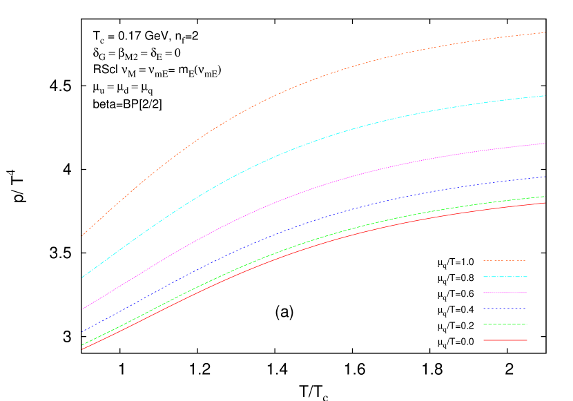
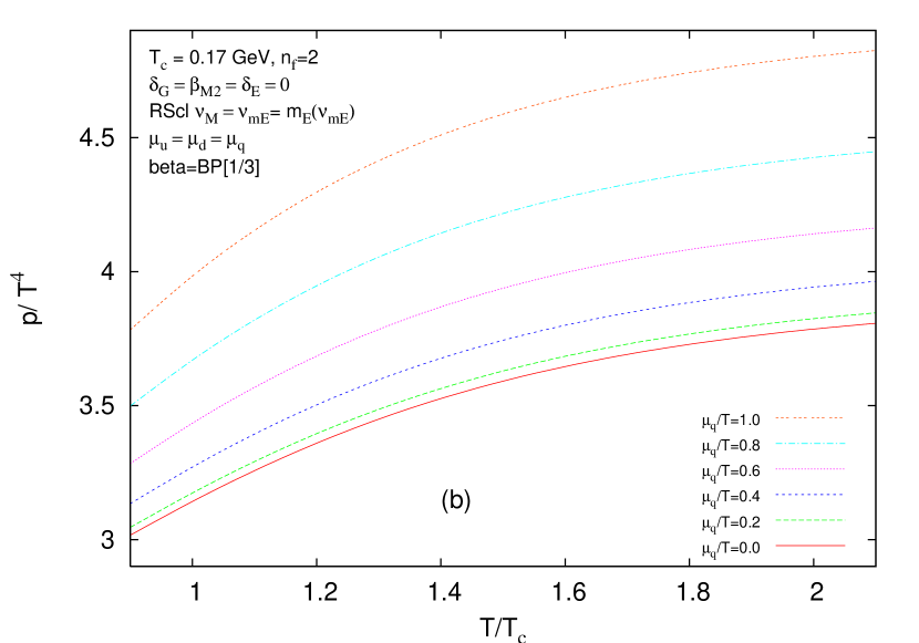
Figure 1: Pressure $p$ (divided by $T^{4}$) as a function of temperature, at various values for the ratios $\mu_{q}/T$ involving the chemical potential $\mu_{q}$ when (a) Borel-Padé BP[2/2] and (b) BP[1/3] is used for the beta function $\beta(g_{s}^{2})$.

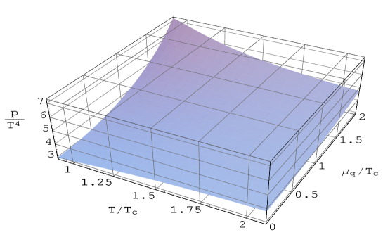
Figure 2: Pressure $p$ (divided by $T^{4}$) as a function of $T/T_{c}$ and $\mu_{q}/T_{c}$ (with: $\mu_{I}=0$). The choice of parameters, RScl’s, and resummation approximants are the same as in Fig. 1(a).

Numerical resummations, performed in the way described above, give us for the total pressure $p={\bar{p}}_{\rm E}+{\bar{p}}_{\rm M+G}$ the results presented in Figs. 1, for various values of the ratio $\mu_{q}/T$ (where $\mu_{q}=\mu_{u}=\mu_{d}$), as a function of temperature in the vicinity of $T_{c}$. Comparison of Figs. 1(a) and (b) further reveals that the results do not change significantly when the type of the BP resummation of the beta function is changed. For better visualization, we present in Fig. 2 a three-dimensional image, showing $p/T^{4}$ as a function of $T/T_{c}$ and of $\mu_{q}/T_{c}$ ($\mu_{I}=0$), for the choice of parameters, RScl’s, and resummation approximants equal to that of Fig. 1(a). Note, however, that in Fig. 2 the second axis is $\mu_{q}/T_{c}$ and not $\mu_{q}/T$ (the latter quantity is kept fixed in the separate curves of Fig. 1(a)).

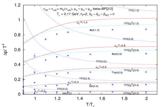
Figure 3: As in Figs. 1, but now for the pressure difference $\Delta p$ divided by $T^{4}$ (solid lines). In addition, the TPS results are included as dotted lines; and the lattice calculation results of Ref. Allton:2005gk are included as crosses, where the depicted error bars include only specific statistical errors.

In Fig. 3 we present the corresponding results for the pressure difference $\Delta p=p(T;\mu_{q})-p(T;\mu_{q}=0)$, for five different values of $\mu_{q}/T$ ($=0.2,0.4,0.6,0.8,1.$). We included, for comparison, the results of the evaluation of the simple truncated perturbation series (TPS) in powers of $g(\nu=2\pi T)$ as dotted lines there. These were obtained by using for ${\bar{p}}_{\rm E}$ the TPS in powers of $g^{2}(\nu=2\pi T)$, and for ${\bar{p}}_{\rm M+G}$ the TPS in powers of $g(\nu=2\pi T)$. The latter TPS is obtained by using expansions (15)-(17) in powers of $g(\nu)$ in expansion (14) for ${\bar{p}}_{\rm M+G}$ (also in the logarithms there), and setting the RScl $\nu=2\pi T$. The unknown parameters $\delta_{\rm E}$, $\delta_{\rm G}$, and $\beta_{\rm M2}$, which affect these TPS’s at ${\cal O}(g^{6})$, were all set equal to zero here. In addition, the TPS’s truncated at ${\cal O}(g^{5})$ are presented, for the aforementioned five values of $\mu_{q}/T$. We note that such types of TPS evaluation (with the common high RScl $\sim 2\pi T$) have been often used in the literature to evaluate $p$ and/or $\Delta p$. The TPS’s presented here do not diverge when approaching even very low values of temperature because for the beta functions we use BP[2/2] (or: BP[1/3] in Fig. 1(b)). Fig. 3 shows that our Padé-related evaluations, while being somewhat higher, reproduce the lattice results for $\Delta p/T^{4}$ to within $20\%$, even at low temperatures $T\approx T_{c}$. On the other hand, the TPS results are very unstable under the change of the truncation order. It appears to be a coincidence that the TPS’s truncated at ${\cal O}(g^{5})$ are in good agreement with the lattice data. Incidentally, the latter TPS’s have values similar to those of ${\cal O}(g^{6})$-TPS’s with $\delta_{\rm E}=-k_{2}$ [in the latter case, ${\bar{p}}_{\rm E}$ has the coefficient at $g^{6}$ equal zero, cf. Eq. (25) and (20)]. Stated otherwise, the ${\cal O}(g^{6})$ TPS’s are quite unstable under the variation of the unknown parameter $\delta_{\rm E}$ while our Padé-related resummations are quite stable (see also Figs. 4 and 5). Furthermore, the TPS results show a strong RScl dependence, as will be shown shortly.

A general remark on the lattice data (included in Fig. 3) and their significance is in order here. The quoted error bars denote only specific statistical errors and do not represent further uncertainties. The aforementioned lattice data have various uncertainties, among them the generic uncertainties of lattice calculations coming from the continuum limit effects (of up to 10%, cf. Allton:2003vx ), from the finite size effects (of about 5%, cf. Gliozzi:2007jh ), and from the uncertainties of the value of $T_{c}$ (of 2-3%). The results for $\Delta p$ for finite chemical potentials suffer from additional problems: since finite $\mu_{q}$-values are treated in Ref. Allton:2005gk by applying a Taylor expansion in powers of $\mu_{q}/T$ (cf. Eq. (3.1) of Ref. Allton:2005gk ), one has to calculate the corresponding coefficients $c_{n}(T)$ – more of them when $\mu_{q}/T$ is higher. In Ref. Allton:2005gk only the first three non-vanishing coefficients ($n=2,4,6$) have been calculated – with high instabilities already for $n=6$ (cf. Fig. 1 in Allton:2005gk ). The error bars in the lattice data in Fig. 3, as well as in Figs. 8-9, present only these specific uncertainties in calculation of the three $c_{n}$’s. However, the terms with $n=8,10,\ldots$ are not included. Consequently, the lattice results for large $\mu_{q}/T$ values ($\mu_{q}/T\geq 0.8$) have to be considered with reservation. An educated guess leads to the expectation that the data in Fig. 3 have an overall uncertainty of around 15%, and probably even higher when $\mu_{q}/T\approx 1$. Therefore, it is fair to say that our predictions are in reasonable agreement with lattice data down to $T=T_{c}$, at least as long as $\mu_{q}<T$. Analogous statements are valid for the comparison with lattice data in Figs. 8 and 9 (see later). What we do not yet understand is the apparent systematics of the lattice results: they lie systematically below our predictions, in particular for high $\mu_{q}$ values. Whether this demonstrates a lattice artefact, possibly connected with the rather large bare quark mass used there, has to be further investigated. In this context, we further note that the difference between our and lattice results could not be significantly reduced by choosing different values for the unknown parameters $\delta_{\rm E}$, $\beta_{\rm M2}$, $\delta_{\rm G}$ (which were set equal to zero in Fig. 3), at least if varying them within the generous ranges specified in Eqs. (24) and (25). In fact, variation of these parameters can decrease our results at $1<T/T_{c}<2$ by less than 1% (see Fig. 5 later).

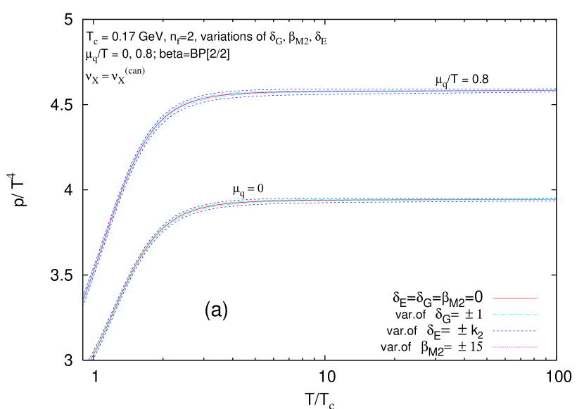
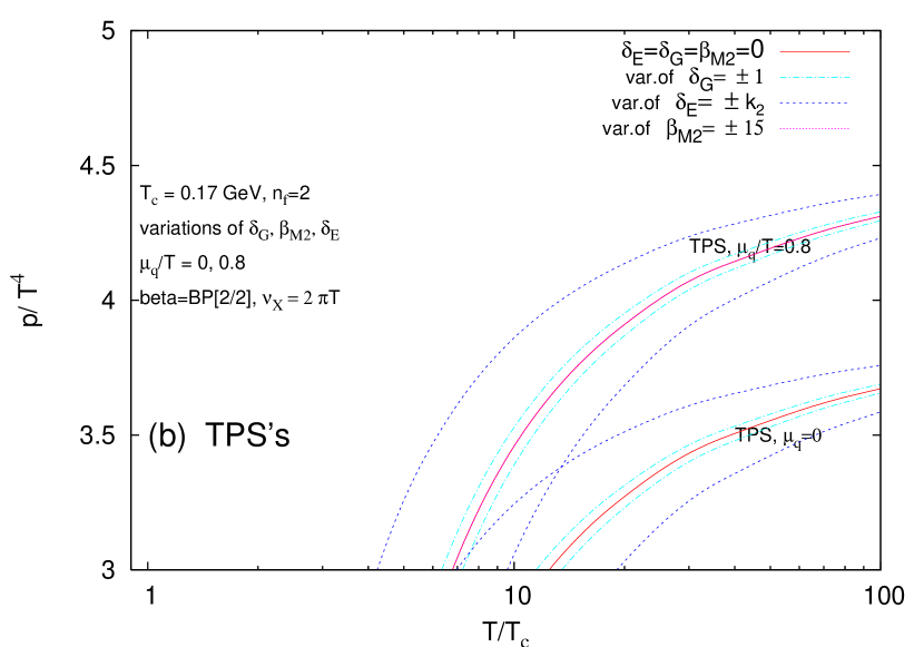
Figure 4: (a) Pressure $p$ (divided by $T^{4}$) as a function of temperature, when the unknown parameters $\delta_{\rm G}$, $\beta_{\rm M2}$ and $\delta_{\rm E}$ are varied according to Eqs. (24) and (25), for two different values of the ratio $\mu_{q}/T$: 0.8 and 0; (b) same as in (a), but for TPS’s (with the common RScl $\nu=2\pi T$).

In Fig. 4(a) we present variations of our results for $p/T^{4}$ in a wide temperature regime when the unknown parameters $\delta_{\rm G}$, $\beta_{\rm M2}$ and $\delta_{\rm E}$ are varied according to Eqs. (24) and (25), for two different fixed values of the ratio $\mu_{q}/T$ ($=0.8,0.$). In Fig. 4(b), the analogous results for the aforementioned simple TPS’s are shown. We see that our results are remarkably stable under the rather generous variations of the three unknown parameters, whereas this is definitely not the case with the TPS’s. The dependence on the unknown parameters $\delta_{\rm E}$ and $\delta_{\rm G}$ is strong in the TPS’s, while the Padé-related resummation results are almost independent of them. The dependence on the parameter $\beta_{\rm M2}$ is too weak to be seen.

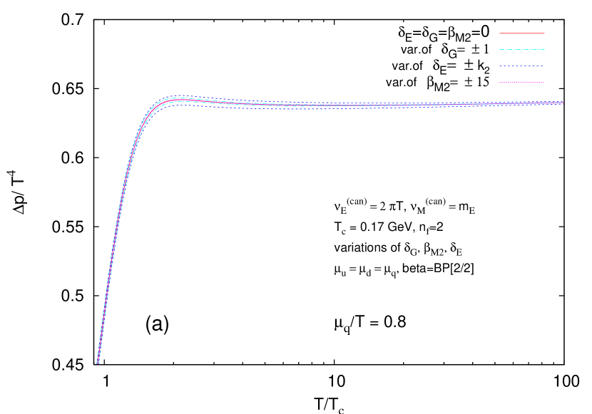
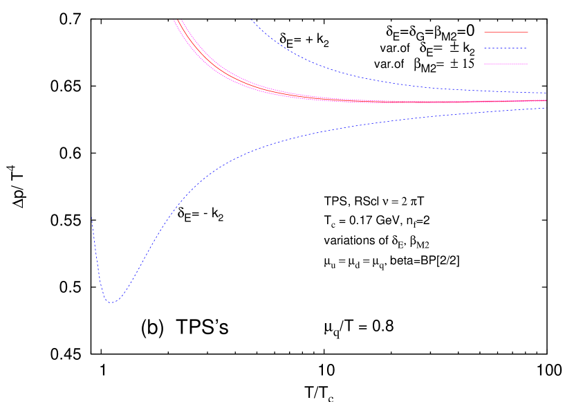
Figure 5: As in Figs. 4, but now for $\Delta p/T^{4}$.

In Figs. 5(a),(b) we present $\Delta p/T^{4}$ in the way completely analogous to the presentation of $p/T^{4}$ in Figs. 4(a),(b). The conclusions for the (in)stability of the calculated $\Delta p$ under the variation of the unknown parameters are similar to those for $p$. The independence of the parameter $\delta_{\rm G}$ in the TPS’s in Fig. 4(b) is a direct consequence of the $\mu_{q}$ independence of $\delta_{\rm G}$. The dependence on the parameter $\beta_{\rm M2}$ is weak in the TPS’s, and too small to be seen in the Padé-type resummation. However, while there is almost no dependence on the unknown parameter $\delta_{\rm E}$ in the Padé-related resummation results, the dependence on $\delta_{\rm E}$ is quite drastic in the TPS’s. This behavior also makes plausible the fact that, by adjusting the value of the unknown parameter $\delta_{\rm E}$, we can, in a way, fine-tune the TPS results to come close to the lattice results (see also Fig. 3).

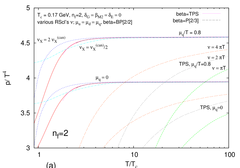
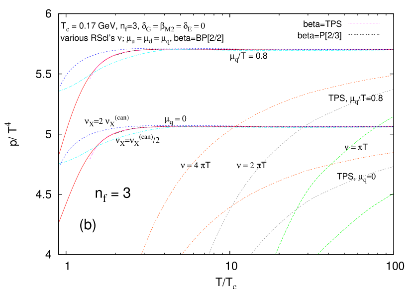
Figure 6: Pressure $p/T^{4}$ as a function of temperature, when the renormalization scales $\nu_{\rm E}$ and $\nu_{\rm M}$ are varied by factor two around the canonical values (27): (a) when $n_{f}=2$; (b) when $n_{f}=3$. The values of the ratios $\mu_{q}/T$ are either $0.8$ or zero. Included are also the corresponding sets of curves with the TPS evaluation.

After having shown that our results are fairly insensitive to the still existing unknown parts of the perturbation series (at $\sim g^{6}$), we now come to the most important results of our approach: the stability under variation of the (two) RScl’s, even at very low temperatures. This is manifested in Figs. 6 and 7.

In Figs. 6(a),(b), we present the behavior of our evaluated results for $p/T^{4}$ when the RScl’s $\nu_{\rm E}$ and $\nu_{\rm M}$ are varied by factor two around the canonical values (27), for $n_{f}=2,3$, respectively. Two sets of curves are given, for $\mu_{q}/T=0.8$ and zero, respectively. In addition, the corresponding sets of curves for the aforementioned simple TPS’s are shown, where now the common RScl $\nu$ is varied from $\pi T$ to $4\pi T$. We see that our evaluated results for $p$ are much more stable under the variation of RScl than the TPS results, down to very low temperatures $T\approx T_{c}$. This is the same conclusion as the one obtained in our previous work GRp for the case of zero chemical potential ($\mu_{q}=0$). For additional comparisons, we included in Figs. 6 the results of our Padé-related evaluation of $p/T^{4}$ with canonical RScl’s (27) when the ${\overline{\rm MS}}$ beta function $\beta(a)$ is (four-loop) TPS, and when it is Padé ${\rm P[2/3]}(a)$. We see that the results in such cases, when they exist, almost coincide with the solid-line curves, i.e., with those with $\beta(a)={\rm BP[2/2]}(a)$. However, due to the Landau singularities of $a(\nu^{2})$ at low RScl’s in the aforementioned cases of $\beta=$ TPS or P[2/3] (cf. Appendix B), the corresponding curves exist (i.e., do not blow up) only down to $T_{\rm min}\approx 1.8T_{c},2.5T_{c}$, respectively (when $n_{f}=3$: $T_{\rm min}\approx 1.4T_{c},2.0T_{c}$, respectively). We note that the curve with $\beta=$ P[2/3] and $\mu_{q}=0$ in Fig. 6(b) corresponds to the central curve with $n_{f}=3$ in Fig. 18 of our previous work GRp and to the upper solid-line curve of Fig. 19 of that work.

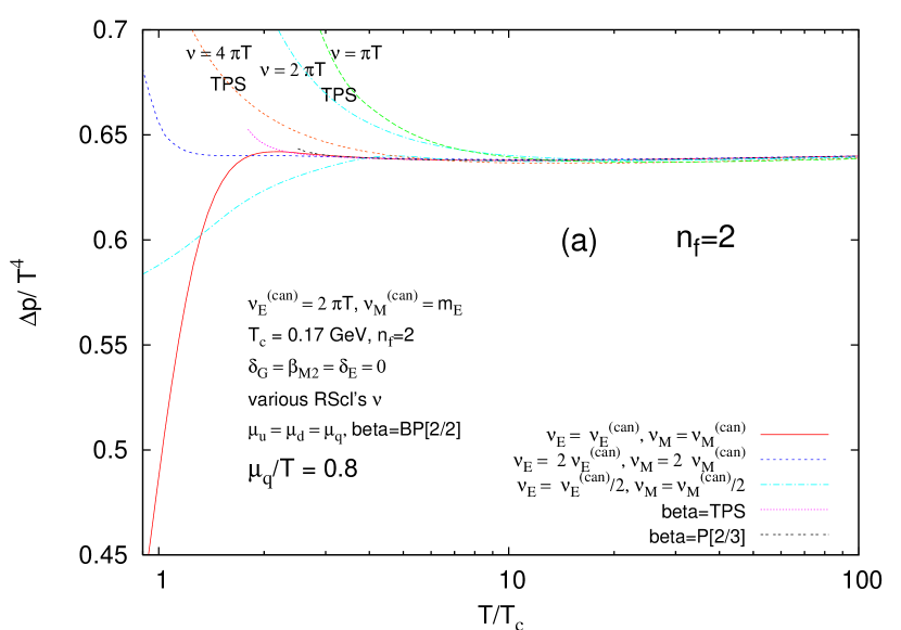
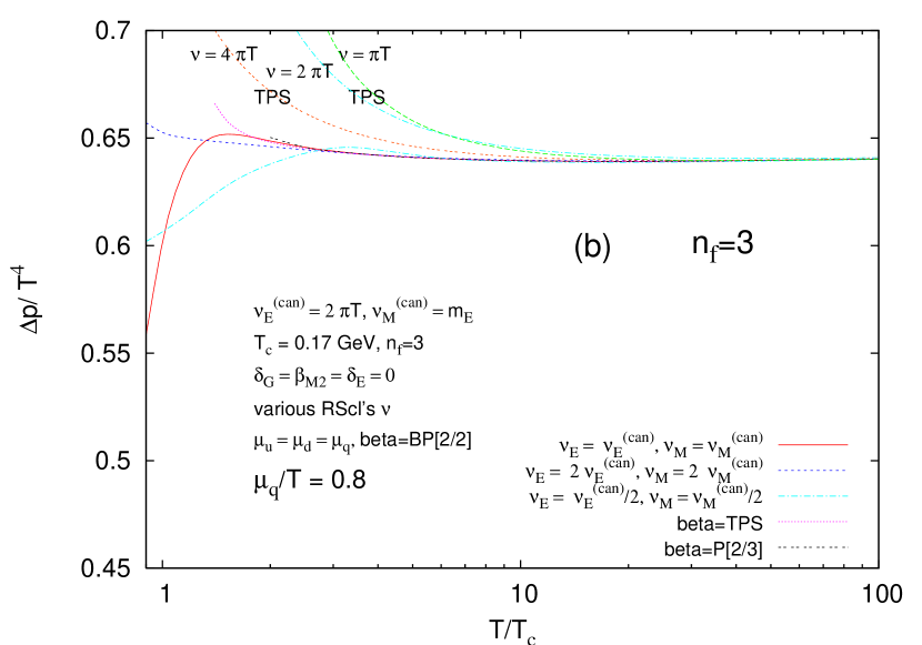
Figure 7: As Figs. 6, but for $\Delta p/T^{4}$ instead of $p/T^{4}$. The chemical potential $\mu_{q}$ has the values $\mu_{q}=0.8T$.

Figs. 7(a),(b) contain similar results for $\Delta p/T^{4}$ (here only for the value $\mu_{q}/T=0.8$). The conclusions about the RScl dependence of the results for $\Delta p/T^{4}$ are virtually the same as for $p/T^{4}$.

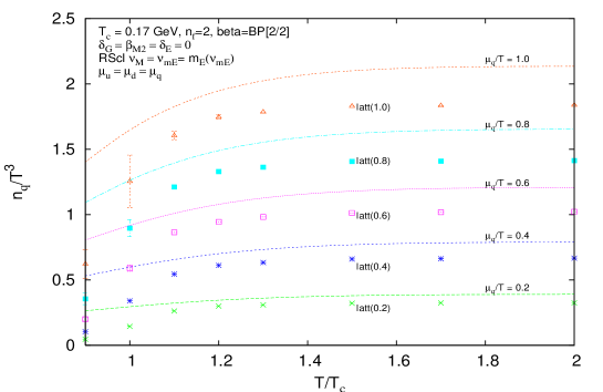
Figure 8: Quark number density $n_{q}$ (divided by $T^{3}$) as a function of $T$, at $\mu_{I}=0$, for various values of the ratio $\mu_{q}/T$. Our results are in the form of curves. Included as points are the corresponding results of the lattice calculation of Ref. Allton:2005gk .

It is exactly this independence of $\nu$ at $T$ down to about $2T_{c}$ which makes our comparison with lattice data (cf. Fig. 3) much more trustworthy than the simple TPS evaluation.

In the remaining part we present results for derived quantities, specifically quark number densities and susceptibilities.

Fig. 8 contains results for the quark number density (32) for various values of $\mu_{q}/T$ ($\mu_{I}=0$). Included are the corresponding results of the lattice calculation of Ref. Allton:2005gk , in the form of points (some with error bars). The values were obtained by numerical differentiation of our results for $p$ with respect to $\mu_{q}$ (with $\mu_{I}=0$ and $T$ constant). Again, we see that our results in general agree with the lattice results to within $20\%$, even at low temperatures $T\approx T_{c}$.

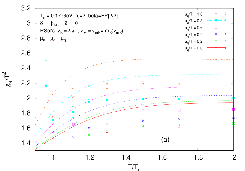
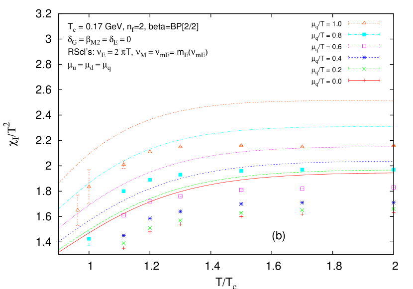
Figure 9: The susceptibilities (a) $\chi_{q}$ and (b) $\chi_{I}$ as a function of temperature, for various values of the ratios $\mu_{q}/T$ ($\mu_{I}=0$). Our results are in the form of curves. Included are the corresponding results of the lattice calculation of Ref. Allton:2005gk , in the form of points (some with error bars).

Finally, in Figs. 9(a),(b) we present the values for the susceptibilities $\chi_{q}$ and $\chi_{I}$ [cf. Eq. (33)] as a function of temperature, for various values of the ratios $\mu_{q}/T$, while keeping $\mu_{I}=0$. The results are presented as various curves, and were obtained, at a given $T$, by numerical evaluation of the double derivatives of our results for the pressure $p$ with respect to $\mu_{q}$ (at constant $\mu_{I}=0$) and with respect to $\mu_{I}$ (around $\mu_{I}=0$, at constant $\mu_{q}$) math . In Figs. 9(a),(b) we included the corresponding results of the lattice calculation of Ref. Allton:2005gk , as points with error bars. Our curves, in general, give results which are by roughly $20\%$ higher than the lattice results.

In addition to the aforementioned susceptibilities, the mixed susceptibility $\chi_{ud}$ which is related to the previous two by

$$\frac{\chi_{I}-\chi_{q}}{T^{2}}=-4\frac{\chi_{ud}}{T^{2}}$$ (34)

has been a subject of interest in the literature. Our numerical results give for the above quantity (34), at $\mu_{I}=0$ (and $n_{f}=2$), values of about $4\times 10^{-3}$ at $\mu_{q}=0$ and at temperatures $1<T/T_{c}<2$ [these values turn negative ($\sim-10^{-3}$) when $\mu_{q}/T=0.2$]. The authors of Ref. Allton:2003vx obtained, by their lattice calculations, for the above quantity (34) at $\mu_{I}=\mu_{q}=0$ (and $n_{f}=2$) decreasing values as the temperature increases from $T_{c}$ to $1.5T_{c}$, and at $T/T_{c}=1.36$ they found a value of $6.6\times 10^{-3}$. Our results for this quantity are roughly in agreement with the lattice results of Refs. Allton:2003vx ; Bernard:2002yd , and with the hard thermal loops (HTL) perturbative estimates of Ref. 3lbebMS . The latter estimates give for the quantity (34), at $1<T/T_{c}<2$, values between $5\times 10^{-3}$ and $1.4\times 10^{-2}$, when using there our values of $a(2\pi T)$ (with the beta function being BP[2/2]). The lattice quenched results of Refs. GG give for this quantity values $\sim 10^{-6}$, i.e., three orders of magnitude lower.

Further, we performed numerical calculations of $p$, $\Delta p$ and $n_{q}$ in the case of three active flavors $n_{f}=3$, with $\mu_{u}=\mu_{d}=\mu_{q}$ ($T$-independent) and $\mu_{s}=0$, with our approach described above. Comparisons with the corresponding lattice calculations of Ref. Fodor:2002km (their Figs. 3 and 6) revealed that, at their values of $\mu_{\rm B}\leq 0.53$ GeV ($\mu_{\rm B}\equiv 3\mu_{q},n_{\rm B}\equiv n_{q}/3$), our results for $\Delta p$ and $n_{\rm B}$ are somewhat higher than theirs, by less than $20\%$ at $T/T_{c}\geq 1.5$, and by $30\%-40\%$ at $T/T_{c}=1.1$. Direct comparison with the lattice results of Ref. Csikor:2004ik is not possible, as no continuum limit correction factor ($c_{\mu}$) was applied there. In Ref. Fodor:2002km , an estimated correction factor $c_{\mu}=0.446$ was applied to $\Delta p$.

IV Summary

Within the present paper we extended our recent approach GRp for improving perturbative expressions for the quark-gluon pressure (obtained by FTPT) to the case of finite (but still small) quark densities. Thereby, the main aim was to find a consistent method for extrapolating the FTPT-based results down to temperatures as low as $T_{c}$ ($\approx 200$ MeV). For such low energies, the original TPS’s are plagued by huge uncertainties, stemming mainly from their strong RScl dependence which itself is partially connected with the occurrence of, at least, two different energy scales contributing to the thermodynamic potential under investigation. Therefore, simple FTP series do not permit a reliable comparison with existing (low energy) lattice data. Such a check can only be performed if the wild RScl dependence is sufficiently tamed. Our method allows such a taming. It rests mainly on two crucial points: Firstly, we performed a careful separation of the low-energy from the high-energy contributions to the pressure, which are responsible for the (in principle measurable) long- and the short-range behavior, respectively. In this way, we can clarify which values of the RScl are the natural ones – they are different for the two parts. Secondly, for each of these contributions we identified Padé-related approximants which – besides showing other physically desirable features – led to (almost) RScl-stable expressions and thus to predictions which can be safely used down to low temperatures. However, the use of the approximants for the low-energy (long-range) contributions at very low temperatures $\sim T_{c}$ is only possible if the unphysical perturbative Landau singularities of the QCD coupling parameter at low energies are eliminated; we did this by using similar Padé-related approximants for the renormalization-group beta function. As a result, we demonstrated that the obtained expressions for the pressure $p$ and the difference $\Delta p=p(\nu_{f})-p(0)$ are fairly insensitive to the (as yet) unknown part of contributions of ${\cal O}(g^{6})$ and to variations of the RScl’s, both of these features being in stark contrast with the TPS expressions.

Our expressions show a surprisingly good agreement with lattice data – not only for the pressure and its $\mu_{f}$ dependence but also for derived quantities, in particular susceptibilities. In this context, we note that the unknown relative deviations of the low temperature lattice results for $p$ and $\Delta p$ from the true values are expected to be roughly in the range of 10-20%. This is due to the well-known lattice artefacts, in particular the ones connected with finite-$\mu_{f}$ effects (truncated Taylor expansion in $\mu_{f}/T$). Our Padé-related evaluations give for $\Delta p/T^{4}$ results which are by not more than 20% higher than the lattice results when $\mu_{q}/T\leq 0.8$ and $1<T/T_{c}<2$, see Fig. 3.

Our approach is valid only for values of the chemical potentials smaller than the temperature, because only in this case dimensional reduction can be applied. Fortunately, present day heavy ion collisions are probing the region with values $\mu_{f}\lesssim 50$ MeV, which are small compared to the temperatures $T\lesssim 5T_{c}$ typically involved. For other kinematic situations, in particular for small $T$ and larger chemical potentials, different reorganizations of perturbation expansions are necessary and have been applied in the literature, the most prominent one being the hard dense loop approximation which is genuinely four-dimensional but based on a non-local effective action Taylor . Recently, a purely diagrammatic calculation of the perturbative QCD pressure (i.e., without involving any effective theory) has been performed Ipp which, at least in principle, should be valid for all kinematic regions. As it should be expected, these results – when applied to high temperatures and (relatively) low chemical potentials – are in accordance with those of the dimensional reduction approach.

Appendix A Relevant coefficients for the pressure at finite chemical potential

Here we compile expressions for parameters $A_{j}$, $m_{\rm E}$ and $g_{\rm E}$ which we obtained from expressions of Ref. Vuo by application of the method of separation of the long-distance from short-distance contributions (i.e., introduction of factorization scale $\Lambda_{\rm E}$: $m_{\rm E}<\Lambda_{\rm E}<2\pi T$), as explained in the beginning of Sec. II. We denote by $\nu$ the renormalization scale (RScl), and $g\equiv g(\nu)$ in ${\overline{\rm MS}}$ scheme. Other notations used in this appendix are:

$${\overline{\mu}}_{f}=\frac{\mu_{f}}{2\pi T}\ ,\qquad z_{f}=\frac{1}{2}-{\rm i}{\overline{\mu}}_{f}\ ,$$ (35)

$${\widetilde{\mu}}_{k}=\frac{1}{n_{f}}\sum_{f}{\overline{\mu}}_{f}^{k},\ {\widetilde{\aleph}}^{(k)}(z)=\frac{1}{n_{f}}\sum_{f}{\overline{\mu}}_{f}^{k}\aleph(z),\ {\widetilde{\aleph}}^{(k)}(\ell,z)=\frac{1}{n_{f}}\sum_{f}{\overline{\mu}}_{f}^{k}\aleph(\ell,z),$$ (36)

$$\ln^{\prime}\zeta(-n)=\frac{\zeta^{\prime}(-n)}{\zeta(-n)}\ ,$$ (37)

where $\aleph(z)$ and $\aleph(\ell,z)$ are the aleph functions defined in Refs. Vuo via digamma functions and derivatives of the Riemann zeta functions.

Coefficients $A_{j}~{}(j=1,...7)$ and $A_{j}^{(\nu)}$, which appear in equations Eqs. (3)-(5) and (8)-(10), and later in Eqs. (15)-(20), are obtained from the “matching parameters” $\alpha_{\rm E_{i}}~{}(i=1,...7)$ in Ref. Vuo by separating appropriately the parts proportional to $\ln\nu_{c}$ ($\ln\bar{\Lambda}$ in Ref. Vuo ), or proportional to $1/\epsilon$, from the remaining ($\nu_{c}$- and $\epsilon$-independent) parts. They take the form

$$A_{1}=\frac{\pi^{2}}{45}\left[8+3n_{f}\left(\frac{7}{4}+30{\widetilde{\mu}}_{2}+60{\widetilde{\mu}}_{4}\right)\right]\ ,$$ (38)

$$A_{2}=-\frac{1}{6}\left[1+\frac{1}{12}n_{f}\left(5+72{\widetilde{\mu}}_{2}+144{\widetilde{\mu}}_{4}\right)\right]\ ,$$ (39)

$$A_{4}=\left[1+\frac{1}{6}n_{f}\left(1+12{\widetilde{\mu}}_{2}\right)\right]\ ,$$ (40)

$$A_{5}=2\left(-\ln 2+\ln^{\prime}\zeta(-1)\right)+\frac{1}{6}n_{f}(1-2\ln 2)(1+12{\widetilde{\mu}}_{2})+4n_{f}{\widetilde{\aleph}}^{(0)}(1,z)\ ,$$ (41)

$$A_{6}={\bigg{\{}}\frac{1}{18}\left[90-396\ln 2+66\gamma_{\rm E}(6+n_{f})+n_{f}(3-42\ln 2)+2n_{f}^{2}(1+2\ln 2)\right]$$

$$~{}~{}+\left[n_{f}{\widetilde{\mu}}_{2}\left(6+44\gamma_{\rm E}-44\ln 2+n_{f}\frac{4}{3}(1+2\ln 2)\right)+\frac{1}{9}n_{f}(n_{f}+6){\widetilde{\aleph}}^{(0)}(z)+n_{f}^{2}\frac{4}{3}{\widetilde{\aleph}}^{(2)}(z)\right]{\bigg{\}}}\ ,$$ (42)

$$A_{7}=\left[22(\gamma_{\rm E}-\ln 2)+1+n_{f}\frac{4}{3}\ln 2+n_{f}\frac{2}{3}{\widetilde{\aleph}}^{(0)}(z)\right]\ ,$$ (43)

$$A_{5}^{(\nu)}=2A_{4}\ ,$$ (44)

$$A_{6}^{(\nu)}=22+\frac{7}{3}n_{f}-\frac{2}{9}n^{2}_{f}+4(11-\frac{2}{3}n_{f})n_{f}{\widetilde{\mu}}_{2}\ ,$$ (45)

$$A_{7}^{(\nu)}=22-\frac{4}{3}n_{f}\ .$$ (46)

The most complicated coefficient is $A_{3}$, which emerges both in Eq. (8) and later in Eq. (20) via the quantity $\kappa$ [Eq. (21)]. It can be expressed as

$$A_{3}=A_{3,1}+A_{3,2}-A_{3}^{(\nu)}\ln 2\ ,$$ (47)

where

$$A_{3,1} = \frac{1}{18}{\Bigg{\{}}3^{2}\left[\frac{116}{5}+4\gamma_{\rm E}-\frac{38}{3}\ln^{\prime}\zeta(-3)+\frac{220}{3}\ln^{\prime}\zeta(-1)\right]$$ (48)

$$+\frac{3}{2}n_{f}{\bigg{[}}\frac{1121}{60}+8\gamma_{\rm E}+2(127+48\gamma_{\rm E}){\widetilde{\mu}}_{2}-644{\widetilde{\mu}}_{4}+\frac{268}{15}\ln^{\prime}\zeta(-3)+\frac{4}{3}(11+156{\widetilde{\mu}}_{2})\ln^{\prime}\zeta(-1)$$

$$+24\left(52{\widetilde{\aleph}}^{(0)}(3,z)+144{\rm i}{\widetilde{\aleph}}^{(1)}(2,z)+17{\widetilde{\aleph}}^{(0)}(1,z)-92{\widetilde{\aleph}}^{(2)}(1,z)+4{\rm i}{\widetilde{\aleph}}^{(1)}(0,z)\right){\bigg{]}}$$

$$+\frac{2}{3}n_{f}{\bigg{[}}\frac{3}{4}(35+472{\widetilde{\mu}}_{2}+1328{\widetilde{\mu}}_{4})-24(1-4{\widetilde{\mu}}_{2})\ln^{\prime}\zeta(-1)$$

$$-144\left(12{\rm i}{\widetilde{\aleph}}^{(1)}(2,z)-2{\widetilde{\aleph}}^{(0)}(1,z)-16{\widetilde{\aleph}}^{(2)}(1,z)-{\rm i}{\widetilde{\aleph}}^{(1)}(0,z)-{\rm i}4{\widetilde{\aleph}}^{(3)}(0,z)\right){\bigg{]}}$$

$$+\frac{1}{4}n_{f}^{2}{\bigg{[}}\frac{1}{3}+4\gamma_{\rm E}+8(7+12\gamma_{\rm E}){\widetilde{\mu}}_{2}+112{\widetilde{\mu}}_{4}-\frac{64}{15}\ln^{\prime}\zeta(-3)-\frac{32}{3}(1+12{\widetilde{\mu}}_{2})\ln^{\prime}\zeta(-1)$$

$$-96\left(8{\widetilde{\aleph}}^{(0)}(3,z)+{\rm i}12{\widetilde{\aleph}}^{(1)}(2,z)-2{\widetilde{\aleph}}^{(0)}(1,z)-4{\widetilde{\aleph}}^{(2)}(1,z)-{\rm i}{\widetilde{\aleph}}^{(1)}(0,z)\right){\bigg{]}}{\Bigg{\}}}\ ,$$

$$A_{3,2} = 4\sum_{f,g}{\bigg{[}}2(1+\gamma_{\rm E}){\overline{\mu}}_{f}^{2}{\overline{\mu}}_{g}^{2}-\aleph(3,z_{f}+z_{g})-\aleph(3,z_{f}+z_{g}^{\ast})-{\rm i}4{\overline{\mu}}_{f}\left(\aleph(2,z_{f}+z_{g})+\aleph(2,z_{f}+z_{g}^{\ast})\right)$$ (49)

$$+4{\overline{\mu}}_{g}^{2}\aleph(1,z_{f})+({\overline{\mu}}_{f}+{\overline{\mu}}_{g})^{2}\aleph(1,z_{f}+z_{g})+({\overline{\mu}}_{f}-{\overline{\mu}}_{g})^{2}\aleph(1,z_{f}+z_{g}^{\ast})+{\rm i}4{\overline{\mu}}_{g}^{2}{\overline{\mu}}_{f}\aleph(0,z_{f}){\bigg{]}}\ ,$$

and

$$A^{\rm(\nu)}_{3} = \left[\left(\frac{97}{3}+\frac{169}{36}n_{f}+\frac{5}{54}n_{f}^{2}\right)+{\widetilde{\mu}}_{2}n_{f}\left(50+\frac{4}{3}n_{f}\right)+{\widetilde{\mu}}_{4}n_{f}\left(-44+\frac{8}{3}n_{f}\right)\right]\ .$$ (50)

The constants $\alpha_{\rm G}$, $\alpha_{\rm M1}$ and $\alpha_{\rm M2}$ were obtained in Ref. KLRS1 :

$$\alpha_{\rm G}=\frac{43}{96}-\frac{157}{6144}\pi^{2}\approx 0.195715,\quad\alpha_{\rm M1}=\frac{43}{32}-\frac{491}{6144}\pi^{2}\approx 0.555017,\quad\alpha_{\rm M2}=-\frac{4}{3}\ ,$$ (51)

and $\beta_{\rm M1}$ in Ref. KLRS2 :

$$\beta_{\rm M1}\approx-1.391512\ .$$ (52)

Appendix B Beta functions of the Borel-Padé type

In this Appendix we present various resummations of the QCD $\beta$ functions as functions of $x=a(Q^{2})=\alpha_{s}(Q^{2})/\pi$, in the ${\overline{\rm MS}}$ scheme. Further, the corresponding running of $a(\nu^{2})$ as function of $x=\nu^{2}$ (in ${\rm GeV}^{2}$) is given, in the various cases, always normalized to $a(m_{\tau}^{2})=0.334/\pi=0.106316$, cf. Eq. (29). We will denote the squared RScl $\nu^{2}$ here as $Q^{2}(\equiv-q^{2}>0)$ to emphasize the space-like character of the corresponding four-vector $q$.

The four-loop renormalization group equation (RGE) for $a(Q^{2})\equiv\alpha_{s}(Q^{2})/\pi$ is:

$$Q^{2}\frac{da(Q^{2})}{Q^{2}}=-\beta_{0}a^{2}(Q^{2})\left[1+c_{1}a(Q^{2})+c_{2}a^{2}(Q^{2})+c_{3}a^{3}(Q^{2})\right]\ ,$$ (53)

where $c_{j}\equiv\beta_{j}/\beta_{0}$ ($j\geq 1$). The one- and two-loop coefficients $\beta_{0}$ and $\beta_{1}$ 1lbe ; 2lbe are scheme independent; in ${\overline{\rm MS}}$ scheme 'tHooft:1973mm the three- and four-loop coefficients $\beta_{2}$ and $\beta_{3}$ were obtained in Refs. 3lbebMS ; 4lbebMS , respectively

$$\beta_{0} = \frac{1}{4}\left(11-\frac{2}{3}n_{f}\right)\ ,\qquad\beta_{1}=\frac{1}{16}\left(102-\frac{38}{3}n_{f}\right)\ ,$$ (54)

$$\beta_{2} = \frac{1}{64}\left(\frac{2857}{2}-\frac{5033}{18}n_{f}+\frac{325}{54}n_{f}^{2}\right)\ ,$$ (55)

$$\beta_{3} = \frac{1}{256}(29243.0-6946.30\ n_{f}+405.089\ n_{f}^{2}+1.49931\ n_{f}^{3})\ ,$$ (56)

and $n_{f}$ is the active number of quark flavors.

The solution of the RGE (53), at low Euclidean energies Q (with either $n_{f}=3$ or $n_{f}=2$) has the known unphysical Landau singularities, i.e., singularities of $a(Q^{2})$ for $Q^{2}\leq Q^{2}_{\rm pole}$. For example, if we choose the realistic value of $\alpha_{s}(Q^{2}=m^{2}_{\tau})=0.334$, the singularity in $a(Q^{2})$ appears already at $Q^{2}_{\rm pole}\approx 0.66^{2}\ {\rm GeV}^{2}\approx 0.44\ {\rm GeV}^{2}$ when $n_{f}=3$, and $Q^{2}_{\rm pole}\approx 0.75^{2}\ {\rm GeV}^{2}\approx 0.57\ {\rm GeV}^{2}$ when $n_{f}=2$ – cf. Figs. 12(a) and 16(a). The main reason for this unphysical behavior of $a(Q^{2})$ is the truncated perturbation series (TPS) form of the beta function $\beta(x=a)$ – the right-hand side of RGE (53). Such a form of $\beta(x)$ has its origin in the perturbative approach (powers of $x=a$). The TPS $|\beta(x)|$ grows out of control when $x=a$ increases – cf. Figs. 10(a) and 14(a). This leads to the appearance of the nonphysical singularities in $a(Q^{2})$ at low positive $Q^{2}\leq Q^{2}_{\rm pole}$.

These singularities prevent us from using, in the traditional perturbative QCD (pQCD), the coupling at squared energies $Q^{2}\lesssim Q^{2}_{\rm pole}$. The problem can be avoided by certain resummations of the TPS $\beta$ function, i.e, by finding such a $\beta(a)$ function whose Taylor expansion around $a=0$ up to $\sim a^{5}$ reproduces the TPS $\beta(a)$ of Eq. (53) and, at the same time, $\beta(a)$ remains more under control when $a$ increases.

One possibility is to construct diagonal or near-to-diagonal Padé approximants based on the TPS $\beta(a)$. For example, the Padé

$${\rm P}[2/3]_{\beta}(a)=-\beta_{0}\frac{a^{2}}{\left[1-c_{1}a+(c_{1}^{2}-c_{2})a^{2}+(-c_{1}^{3}+2c_{1}c_{2}-c_{3})a^{3}\right]}$$ (57)

gives us an expression which, up to $a\approx 0.3$, behaves well – cf. Figs. 10(b) and 14(b). However, around $a\approx 0.3$, this $\beta(a)$ goes abruptly out of control, because the Padé expression has a pole there. The corresponding running coupling $a(x=Q^{2})$ achieves singularity already at $Q_{\rm pole}^{2}\approx 0.81^{2}\ {\rm GeV^{2}}\approx 0.65\ {\rm GeV^{2}}$ for $n_{f}=3$, and $Q_{\rm pole}^{2}\approx 0.92^{2}\ {\rm GeV^{2}}\approx 0.85\ {\rm GeV^{2}}$ for $n_{f}=2$ – cf. Figs. 12(b) and 16(b). In contrast to the TPS $\beta(a)$ case, however, $a(Q^{2})$ seems to be well under control now for virtually all $Q^{2}$ larger than $Q_{\rm pole}^{2}$.

Another possibility, which avoids the aforementioned pole problem of the Padé $\beta(x=a)$, would go in the direction of resumming first the Borel transform ${\rm B}_{\beta}(y)$ (the latter has in general significantly weaker singularities than $\beta$), and then applying the inverse transformation via a Borel integration. For example, we can try to apply diagonal or close-to-diagonal Padé resummation to ${\rm B}_{\beta}(y)$. The Borel transform is

$${\rm B}_{\beta}(y) = -\beta_{0}\left(\frac{y}{1!}+c_{1}\frac{y^{2}}{2!}+c_{2}\frac{y^{3}}{3!}+c_{3}\frac{y^{4}}{4!}+\cdots\right)\ ,$$ (58)

and the Padé P[2/2] and P[1/3] resummations of the above TPS are

$${\rm P[2/2]_{B}}(y) = -\beta_{0}\frac{y+r_{2}y^{2}}{1+t_{1}y+t_{2}y^{2}}\ ,$$ (59)

$${\rm P[1/3]_{B}}(y) = -\beta_{0}\frac{y}{1+s_{1}y+s_{2}y^{2}+s_{3}y^{3}}\ ,$$ (60)

where the coefficients $r_{j},t_{j},s_{j}$ are unique functions of $c_{k}$’s such that reexpansion of (59) and (60) reproduces expansion (58) up to (and including) $\sim y^{4}$ term:

$$r_{2} = (1/2)(3c_{1}^{3}-4c_{1}c_{2}+c_{3})/\xi\ ,$$

$$t_{1} = (1/2)(-2c_{1}c_{2}+c_{3})/\xi\ ,\qquad t_{2}=(1/12)(4c_{2}^{2}-3c_{1}c_{3})/\xi\ ,$$ (61)

$$s_{1} = (1/2)c_{1}\ ,\qquad s_{2}=(1/12)(3c_{1}^{2}-2c_{2})\ ,\qquad s_{3}=(1/24)(-3c_{1}^{3}+4c_{1}c_{2}-c_{3})\ ,$$ (62)

and we used the notation $\xi=(3c_{1}^{2}-2c_{2})$. However, the inverse Borel transformation

$$\beta(x)=\int_{0}^{\infty}dy\ \exp(-y/x){\rm B}_{\beta}(y)$$ (63)

cannot be constructed by inserting here directly the Padé expressions (59) or (60) for the integrand. This is so because the latter expressions have poles on the positive axis: ${\rm P[2/2]_{B}}(y)$ at $y_{\rm p.}\approx 1.13,1.01$ for $n_{f}=3,2$, respectively; ${\rm P[1/3]_{B}}(y)$ at $y_{\rm p.}\approx 0.94,0.88$ for $n_{f}=3,2$, respectively. These “infrared renormalon” singularities imply ambiguities in the integration: $\delta\beta(a)\sim\exp(-y_{\rm p.}/a)$ [$\sim\delta(Q^{2}da(Q^{2})/dQ^{2})\sim\delta a(Q^{2})$]. This implies an ambiguity in the coupling $a(Q^{2})$: $\delta a(Q^{2})\sim({\Lambda^{2}_{\rm{\overline{MS}}}}/Q^{2})^{\beta_{0}y_{\rm p.}}\equiv({\Lambda^{2}_{\rm{\overline{MS}}}}/Q^{2})^{\eta}$. Numerically, for ${\rm P[2/2]_{B}}$, $\eta\approx 2.55,2.44$ for $n_{f}=3,2$, respectively; for ${\rm P[1/3]_{B}}$, $\eta\approx 2.11,2.13$ for $n_{f}=3,2$, respectively. We can fix the above ambiguity by choosing a specific recipe for the Borel integration over the pole $y_{\rm p.}$. We will choose the Principal Value (PV) prescription

$${\rm BP}[i/j]_{\beta}(x)={\rm Re}\int_{\pm i\varepsilon}^{\infty\pm i\varepsilon}dy\ \exp(-y/x){\rm P}[i/j]_{\rm B}(y)\ ,$$ (64)

where $[i/j]=[2/2]$ or $[1/3]$. Numerically, this is difficult to implement, as $\varepsilon\to+0$ and we approach the pole $y_{\rm p.}$ down to the distance ${\varepsilon}$ during the integration. However, we can use the Cauchy theorem, and the fact that the Borel transforms (59) and (60) do not have any poles in the complex semiplane ${\rm Re}(y)\geq 0$ except the aforementioned $y_{\rm p.}>0$. This allows us to avoid the vicinity of the pole, for example by integrating along a ray $y=r\exp(-i\phi)$, where $\phi$ is any small but finite positive fixed angle (cf. Refs. Cvetic:2001sn ; GRp )

$${\rm BP}[i/j]_{\beta}(x) = {\rm Re}{\Big{\{}}\exp(-i\phi)\int_{r=0}^{\infty}dr\exp(-y/x){\rm P}[i/j]_{\rm B}(y)\Big{|}_{y=r\exp(-i\phi)}{\Big{\}}}\ .$$ (65)

This approach, which is numerically stable, gives us for the Borel-Padé(BP)-resummed $\beta(x)$-functions values which are surprisingly non-singular and achieve at $x\equiv a\approx 1.$ value zero (infrared fixed point) – cf. Figs. 11 and 15. Integration of the RGE with these BP-resummed four-loop ${\rm{\overline{MS}}}$ $\beta$ functions, with the phenomenologically acceptable initial condition $\alpha_{s}(m^{2}_{\tau})=0.334$ [Eq. (29)], gives us $a(x=Q^{2})$ running couplings which are presented in Figs. 13 and 17. Both choices BP[2/2] and BP[1/3] give similar behavior for $a(Q^{2})$. There are no Landau singularities present any more, and the coupling is analytic in the sense that there are no unphysical singularities on the space-like axis of the squared momenta $q^{2}\equiv-Q^{2}$. Furthermore, due to the aforementioned zero of the BP $\beta$ functions, the coupling $a(Q^{2})$ remains finite down to $Q^{2}=0$ where it has a value $\approx 1$. The obtained “analytized” coupling $a(Q^{2})$ probably represents a version of analytic QCD. Therefore, the skeleton-motivated method of Refs. GCCV can be applied as a alternative way of evaluating the low-energy QCD observables.

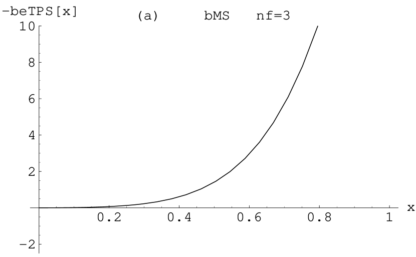
Figure 10: ${\overline{\rm MS}}$ beta functions $-\beta(x)/\beta_{0}$, for $n_{f}=3$, whose TPS is ${\rm TPS}(x)=1+c_{1}x+c_{2}x^{2}+c_{3}x^{3}$: (a) TPS(x), and (b) Padé P[2/3](x) cases; $x$ here stands for $a(Q^{2})$.

Figure 11: ${\overline{\rm MS}}$ beta functions $-\beta(x)/\beta_{0}$, for $n_{f}=3$, whose expansion is $(1+c_{1}x+c_{2}x^{2}+c_{3}x^{3})$: (a) Borel-Padé BP[2/2](x), and (b) BP[1/3](x) cases; $x$ here stands for $a(Q^{2})$.

Figure 12: ${\overline{\rm MS}}$ running of $a(x=Q^{2})$, for $n_{f}=3$, when the beta functions are (a) TPS, and (b) Padé P[2/3].

Figure 13: ${\overline{\rm MS}}$ running of $a(x=Q^{2})$, for $n_{f}=3$, when the beta functions are (a) Borel-Padé BP[2/2], and (b) BP[1/3].

Figure 14: ${\overline{\rm MS}}$ beta functions $-\beta(x)/\beta_{0}$, for $n_{f}=2$, whose TPS is ${\rm TPS}(x)=1+c_{1}x+c_{2}x^{2}+c_{3}x^{3}$: (a) TPS(x), and (b) Padé P[2/3](x) cases; $x$ here stands for $a(Q^{2})$.

Figure 15: ${\overline{\rm MS}}$ beta functions $-\beta(x)/\beta_{0}$, for $n_{f}=2$, whose expansion is $(1+c_{1}x+c_{2}x^{2}+c_{3}x^{3})$: (a) Borel-Padé BP[2/2](x), and (b) BP[1/3](x) cases; $x$ here stands for $a(Q^{2})$.

Figure 16: ${\overline{\rm MS}}$ running of $a(x=Q^{2})$, for $n_{f}=2$, when the beta functions are (a) TPS, and (b) Padé P[2/3].

Figure 17: ${\overline{\rm MS}}$ running of $a(x=Q^{2})$, for $n_{f}=2$, when the beta functions are (a) Borel-Padé BP[2/2], and (b) BP[1/3].

References

- (1) Z. Fodor and S. D. Katz, Phys. Lett. B 534, 87 (2002) [hep-lat/0104001]; JHEP 0203, 014 (2002) [hep-lat/0106002].
- (2) C. R. Allton et al., Phys. Rev. D 66, 074507 (2002) [hep-lat/0204010]; C. R. Allton et al., Nucl. Phys. Proc. Suppl. 119, 538 (2003) [hep-lat/0209012].
- (3) P. de Forcrand and O. Philipsen, Nucl. Phys. B 642, 290 (2002) [hep-lat/0205016]; M. D’Elia and M. P. Lombardo, Phys. Rev. D 67, 014505 (2003) [hep-lat/0209146].
- (4) S. Kratochvila and P. de Forcrand, Nucl. Phys. Proc. Suppl. 140, 514 (2005) [hep-lat/0409072].
- (5) K. Kajantie, M. Laine, K. Rummukainen and Y. Schröder, Phys. Rev. D 67, 105008 (2003) [hep-ph/0211321].
- (6) A. Vuorinen, Phys. Rev. D 68, 054017 (2003) [hep-ph/0305183]; hep-ph/0402242; Phys. Rev. D 67, 074032 (2003) [hep-ph/0212283].
- (7) George A. Baker, Jr. and Peter Graves-Morris, Padé Approximants, 2nd edition, (Encyclopedia of Mathematics and Its Applications, Vol. 59), edited by Gian-Carlo Rota (Cambridge University Press, 1996).
- (8) E. Gardi, Phys. Rev. D 56, 68 (1997) [hep-ph/9611453].
- (9) G. Cvetič, Nucl. Phys. B 517, 506 (1998) [hep-ph/9711406]; Phys. Rev. D 57, R3209 (1998) [hep-ph/9711487]; Nucl. Phys. Proc. Suppl. 74, 333 (1999) [hep-ph/9808273]; G. Cvetič and R. Kögerler, Nucl. Phys. B 522, 396 (1998) [hep-ph/9802248].
- (10) G. Cvetič, Phys. Lett. B 486, 100 (2000) [hep-ph/0003123]; G. Cvetič and R. Kögerler, Phys. Rev. D 63, 056013 (2001) [hep-ph/0006098].
- (11) G. Cvetič and R. Kögerler, Phys. Rev. D 70, 114016 (2004) [hep-ph/0406028]; Phys. Rev. D 66, 105009 (2002) [hep-ph/0207291].
- (12) D. J. Gross, R. D. Pisarski and L. G. Yaffe, Rev. Mod. Phys. 53, 43 (1981); T. Appelquist and R. D. Pisarski, Phys. Rev. D 23, 2305 (1981).
- (13) E. Braaten and A. Nieto, Phys. Rev. Lett. 76, 1417 (1996) [hep-ph/9508406]; Phys. Rev. D 53, 3421 (1996) [hep-ph/9510408].
- (14) A. Hart, M. Laine and O. Philipsen, Nucl. Phys. B 586, 443 (2000) [hep-ph/0004060].
- (15) F. Di Renzo, M. Laine, V. Miccio, Y. Schröder and C. Torrero, JHEP 0607, 026 (2006) [hep-ph/0605042].
- (16) S. Nadkarni, Phys. Rev. D 38, 3287 (1988).
- (17) N. P. Landsman, Nucl. Phys. B 322, 498 (1989).
- (18) B. V. Geshkenbein, B. L. Ioffe and K. N. Zyablyuk, Phys. Rev. D 64, 093009 (2001) [hep-ph/0104048].
- (19) G. Cvetič and T. Lee, Phys. Rev. D 64, 014030 (2001) [hep-ph/0101297]; G. Cvetič, C. Dib, T. Lee and I. Schmidt, Phys. Rev. D 64, 093016 (2001) [hep-ph/0106024].
- (20) C. R. Allton, S. Ejiri, S. J. Hands, O. Kaczmarek, F. Karsch, E. Laermann and C. Schmidt, Phys. Rev. D 68, 014507 (2003) [hep-lat/0305007].
- (21) C. R. Allton et al., Phys. Rev. D 71, 054508 (2005) [hep-lat/0501030].
- (22) Z. Fodor, S. D. Katz and K. K. Szabo, Phys. Lett. B 568, 73 (2003) [hep-lat/0208078].
- (23) F. Csikor, G. I. Egri, Z. Fodor, S. D. Katz, K. K. Szabo and A. I. Toth, JHEP 0405, 046 (2004) [hep-lat/0401016].
- (24) Mathematica 5.2, Wolfram Research, Inc.
- (25) F. Gliozzi, hep-lat/0701020.
- (26) C. Bernard et al. [MILC Collaboration], Nucl. Phys. Proc. Suppl. 119, 523 (2003) [hep-lat/0209079].
- (27) J. P. Blaizot, E. Iancu and A. Rebhan, Phys. Lett. B 523, 143 (2001) [hep-ph/0110369].
- (28) R. V. Gavai, S. Gupta and P. Majumdar, Phys. Rev. D 65, 054506 (2002) [hep-lat/0110032]; Phys. Rev. D 67, 034501 (2003) [hep-lat/0211015]; Phys. Rev. D 68, 034506 (2003) [hep-lat/0303013].
- (29) J. C. Taylor and S. M. H. Wong, Nucl. Phys. B 346, 115 (1990); E. Braaten and R. D. Pisarski, Phys. Rev. D 45, 1827 (1992).
- (30) A. Ipp, K. Kajantie, A. Rebhan and A. Vuorinen, Phys. Rev. D 74, 045016 (2006) [hep-ph/0604060].
- (31) K. Kajantie, M. Laine, K. Rummukainen and Y. Schröder, JHEP 0304, 036 (2003) [hep-ph/0304048].
- (32) D. J. Gross and F. Wilczek, Phys. Rev. Lett. 30, 1343 (1973); H. D. Politzer, Phys. Rev. Lett. 30, 1346 (1973).
- (33) W. E. Caswell, Phys. Rev. Lett. 33, 244 (1974); D. R. T. Jones, Nucl. Phys. B 75, 531 (1974); E. Egorian and O. V. Tarasov, Theor. Math. Phys. 41, 863 (1979) [Teor. Mat. Fiz. 41, 26 (1979)].
- (34) G. ’t Hooft, Nucl. Phys. B 61, 455 (1973).
- (35) O. V. Tarasov, A. A. Vladimirov and A. Y. Zharkov, Phys. Lett. B 93 (1980) 429; S. A. Larin and J. A. M. Vermaseren, Phys. Lett. B 303, 334 (1993) [hep-ph/9302208].
- (36) T. van Ritbergen, J. A. M. Vermaseren and S. A. Larin, Phys. Lett. B 400, 379 (1997) [hep-ph/9701390].
- (37) G. Cvetič and C. Valenzuela, Phys. Rev. D 74, 114030 (2006) [hep-ph/0608256]; J. Phys. G 32, L27 (2006) [hep-ph/0601050].