UWThPh-2006-29
A renormalizable $SO(10)$ GUT scenario
with spontaneous CP violation

Abstract

We consider fermion masses and mixings in a renormalizable SUSY $SO(10)$ GUT with Yukawa couplings of scalar fields in the representation $\mathbf{10}\oplus\mathbf{120}\oplus\overline{\mathbf{126}}$. We investigate a scenario defined by the following assumptions: i) A single large scale in the theory, the GUT scale. ii) Small neutrino masses generated by the type I seesaw mechanism with negligible type II contributions. iii) A suitable form of spontaneous CP breaking which induces hermitian mass matrices for all fermion mass terms of the Dirac type. Our assumptions define an 18-parameter scenario for the fermion mass matrices for 18 experimentally known observables. Performing a numerical analysis, we find excellent fits to all observables in the case of both the normal and inverted neutrino mass spectrum.

1 Introduction

The group $SO(10)$ is a favourite candidate for grand unified theories (GUTs) [1] because its 16-dimensional irreducible representation (irrep), the spinor representation, contains all chiral fermions included in a Standard Model (SM) family plus an additional neutrino SM gauge singlet. Moreover, such theories allow for type I [2] and type II [3] seesaw mechanisms (see also [4]) for the light neutrino masses. In the construction of $SO(10)$ theories, there are two options [5], either using low-dimensional scalar irreps but accepting non-renormalizable terms in the Lagrangian, or one sticks to renormalizable terms, then one has to accept high-dimensional scalar irreps according to [6, 7]

$$\mathbf{16}\otimes\mathbf{16}=\left(\mathbf{10}\oplus\mathbf{126}\right)_{\mathrm{S}}\oplus\mathbf{120}_{\mathrm{AS}},$$ (1)

where the subscripts “S” and “AS” denote, respectively, the symmetric and antisymmetric parts of the tensor product.

In this paper, we deal with the second option. A special renormalizable model is the so-called “minimal SUSY $SO(10)$ GUT” (MSGUT) [8], which uses, for the Yukawa couplings, one scalar in the $\mathbf{10}$ and one in the $\overline{\mathbf{126}}$ irrep in order to account for all fermion masses and mixings; it contains, in addition, one $\mathbf{210}$ and one $\mathbf{126}$ scalar irrep, in order to perform the suitable symmetry breakings. This model has built-in the gauge-coupling unification of the minimal SUSY extension of the Standard Model (MSSM). Detailed studies of this minimal theory have been performed [9, 10], also with small effects of the 120-plet [11]. Though the MSGUT works very well in the fermion sector, there is a tension between the scale of the light neutrino masses and the GUT scale. The reason is that the natural order of the neutrino masses in GUTs is $v^{2}/M_{\mathrm{GUT}}\sim 1.5\times 10^{-3}$ eV, where we have used $v\sim 174$ GeV for the electroweak scale and a GUT scale of $M_{\mathrm{GUT}}\sim 2\times 10^{16}$ GeV. This neutrino mass scale is too low because $\sqrt{\Delta m^{2}_{\mathrm{atm}}}\sim 0.05$ eV where $\Delta m^{2}_{\mathrm{atm}}$ is the atmospheric neutrino mass-squared difference—for reviews on the status of neutrino masses and mixing see [13, 14]. Studies of the heavy scalar states [12], together with studies of the fermion mass spectrum, have shown that the MSGUT is too constrained [15], and the tension between the scale of light neutrino masses and the GUT scale cannot be overcome: if one has a good fit of the fermion masses, which requires a seesaw scale below $M_{\mathrm{GUT}}$, then the gauge coupling unification of the MSSM [16, 17] is spoiled.

A natural step for supplying additional degrees of freedom to the MSGUT is to add the 120-plet of scalars [18] which appears anyway in Eq. (1)—for early works in this direction see [19, 20, 21, 22]. The disadvantage is that this step adds a considerable number of parameters and reduces the predictability of the theory. Adding the $\mathbf{120}$ leads to a resurgence of the type I seesaw mechanism [10], as a consequence of the collapse of the seesaw scale with the GUT scale, because type I seesaw allows to enhance the neutrino masses through small Yukawa couplings of the $\overline{\mathbf{126}}$ [18, 24, 25]; without the $\mathbf{120}$, i.e. in the MSGUT, this process leads to the contradictions mentioned above.

The $\mathbf{120}$ has electrically neutral components only in its four doublets with respect to the SM gauge group. These contribute to the Higgs doublets $H_{d}$, $H_{u}$ of the MSSM, which are assumed to be the only light scalar degrees of freedom and the only ones which acquire VEVs at the electroweak scale. Thus the MSGUT enlarged by the $\mathbf{120}$ inherits, from the MSGUT, the scalar fields responsible for spontaneous symmetry breaking above the electroweak scale. In [24] we took this into account by explicitly making the identification

$$w_{R}=M_{\mathrm{GUT}}=2\times 10^{16}\>\mbox{GeV},$$ (2)

where $w_{R}$, which defines the seesaw scale, is the vacuum expectation value (VEV) of $(\mathbf{10},\mathbf{1},\mathbf{3})\in\overline{\mathbf{126}}$, with the usual notation for multiplets of the Pati–Salam subgroup [26] $SU(4)_{c}\times SU(2)_{L}\times SU(2)_{R}$ of $SO(10)$. Furthermore, in that paper we reduced the number of parameters in the fermion mass matrices by assuming a horizontal $\mathbbm{Z}_{2}$ symmetry and spontaneous CP violation, i.e. real Yukawa couplings, with CP violation stemming from the phases of the VEVs. We showed numerically that this scenario can excellently reproduce the known fermion masses and mixings.

Recently, the role of spontaneous CP violation has been upgraded. A “New MSGUT” (NMSGUT) was proposed [27], defined by extending the MSGUT by the $\mathbf{120}$ and spontaneous CP violation. It was shown that the requirement of spontaneous CP violation not only has the virtue of reducing the number of parameters of the theory but it has an important impact, via threshold effects, on the unification scale as well; it tends to raise the unification scale and with it the masses of all heavy multiplets, thereby suppressing baryon decay.

In the present paper we retain Eq. (2) as a reference point. We do not employ any horizontal symmetry but we again motivate real Yukawa coupling matrices by spontaneous CP violation. However, we assume that it is of a very specific kind: CP is solely violated by imaginary VEVs of the $\mathbf{120}$; the VEVs of the $\mathbf{10}$ and $\overline{\mathbf{126}}$ are assumed to be real. In this way, the mass matrices of the down-quarks, up-quarks, charged leptons and the neutrino Dirac-mass matrix are hermitian. This scenario was originally proposed in [21], its compatibility with sufficiently slow proton decay shown in [22]. However, in [21, 22] it was assumed that the type II seesaw mechanism is dominating. Since this is incompatible with having only one large scale, we have in the present paper type I dominance and neglect possible small contributions of type II, suppressed by $v^{2}/M_{\mathrm{GUT}}$. Our scenario gives an excellent fit to all known fermion masses, mixings and the CKM phase $\delta_{\mathrm{CKM}}$, as good as the one in [24], though it is of a rather different type. This shows that the fermion data do not fix the enlarged MSGUT in a unique way and there is considerable freedom in reducing the number of parameters in this theory.

The paper is organized as follows. In Section 2 we discuss CP-invariant Yukawa couplings and lay out our scenario. The method and results of our numerical analysis are discussed in Section 3. In Section 4 we present the conclusions. Appendix A contains a small collection of formulas for the $SO(10)$ spinor representation, which is helpful for Section 2.

2 An $SO(10)$ scenario motivated by spontaneous CP violation

Let us a define a transformation

$$\mbox{CP:}\quad\begin{array}[]{ccl}\psi_{L}(x)&\to&i\,C\psi_{L}^{*}(\hat{x}),\\[2.84526pt] W^{pq}_{\mu}(x)&\to&\varepsilon(\mu)\eta_{pq}W^{pq}_{\mu}(\hat{x}),\end{array}$$ (3)

where $\psi_{L}$ is a fermionic 16-plet, $C$ is the charge-conjugation matrix, the 45 gauge fields are denoted by $W^{pq}_{\mu}$ ($p<q$), $\varepsilon(\mu)=1$ for $\mu=0$ and $-1$ for $\mu=1,\,2,\,3$, $\hat{x}=(x^{0},-\vec{x})$, and the $\eta_{pq}$ are signs. No summation is implied in Eq. (3). The 45 (hermitian) generators of the gauge group $SO(10)$ in the fermionic $\mathbf{16}$ are given by

$$\frac{i}{2}\sigma_{pq}=\frac{i}{2}\,\Gamma_{p}\Gamma_{q}\quad(1\leq p<q\leq 10).$$ (4)

For a representation of the operators $\Gamma_{p}$ ($p=1,\ldots,10)$ of the Clifford algebra and useful formulas concerning the spinor irrep $\mathbf{16}$ see Appendix A. One can easily check that the gauge interaction of the fermionic 16-plet is invariant under the transformation (3) if [7, 28, 29]

$$-\sigma_{pq}^{T}\,\eta_{pq}=\sigma_{pq}.$$ (5)

Since

$$\Gamma_{p}^{T}=\xi_{p}\Gamma_{p}\quad\mbox{with}\quad\xi_{p}=(-1)^{1+p},$$ (6)

one finds

$$\eta_{pq}=\xi_{p}\xi_{q}=(-1)^{p+q}.$$ (7)

Denoting the generators of the Lie algebra $so(10)$ by $M_{pq}$, we mention that

$$M_{pq}\to\eta_{pq}\,M_{pq}=SM_{pq}S\quad\mbox{with}\quad S=\mbox{diag}\,(1,-1,1,-1,1,-1,1,-1,1,-1)$$ (8)

is the automorphism associated with root reflection, which is the canonical automorphism associated with CP. Such an automorphism exists for all compact Lie groups and is the reason why any gauge Lagrangian, whether for fermions or scalars, is CP-invariant [7, 28, 29].

Now we transfer the CP transformation to the Yukawa couplings given by the Lagrangian

$$\mathcal{L}_{Y} = \frac{1}{2}\left(H_{ab}\,\psi_{aL}^{T}C^{-1}\mathcal{B}\,\Gamma_{p}H_{p}\psi_{bL}+G_{ab}\,\psi_{aL}^{T}C^{-1}\mathcal{B}\,\Gamma_{p}\Gamma_{q}\Gamma_{r}D_{pqr}\psi_{bL}+\right.$$ (9)

$$\left.\hphantom{xxi}F_{ab}\,\psi_{aL}^{T}C^{-1}\mathcal{B}\,\Gamma_{p}\Gamma_{q}\Gamma_{r}\Gamma_{s}\Gamma_{t}{\bar{\Delta}}_{pqrst}\psi_{bL}\right)+\mbox{H.c.}$$

The indices $a$, $b$ denote the family indices, $p,\,q,\,r,\,s,\,t=1,\ldots,10$ are $SO(10)$ indices, and $C$ is the charge-conjugation matrix. Summation over family and $SO(10)$ indices is implied in Eq. (9). The matrix $\mathcal{B}$, which ensures $SO(10)$ invariance, is defined in Eq. (A6). The Yukawa coupling matrices have the properties

$$H_{ab}=H_{ba},\quad G_{ab}=-G_{ba},\quad F_{ab}=F_{ba}.$$ (10)

We define CP transformations (no summations implied)

$$H_{p}(x) \to \xi_{p}H_{p}^{*}(\hat{x}),$$ (11)

$$D_{pqr}(x) \to \xi_{p}\xi_{q}\xi_{r}D_{pqr}^{*}(\hat{x}),$$ (12)

$$\bar{\Delta}_{pqrst}(x) \to \xi_{p}\xi_{q}\xi_{r}\xi_{s}\xi_{t}\bar{\Delta}_{pqrst}^{*}(\hat{x}),$$ (13)

for the scalar fields of the irreps $\mathbf{10}$, $\mathbf{120}$ and $\overline{\mathbf{126}}$, respectively; the latter two are totally antisymmetric tensor fields, $\bar{\Delta}$ is self-dual in addition.

Now we require invariance of the Lagrangian (9) under the CP transformation given by Eqs. (3), (11), (12) and (13). As an example we take the $\mathbf{10}$ and obtain

$$H_{ab}\,\psi_{aL}^{T}\mathcal{B}C^{-1}\Gamma_{p}H_{p}\psi_{bL}\stackrel{{\scriptstyle\mathrm{CP}}}{{\to}}-H_{ab}\,\psi_{aL}^{\dagger}\mathcal{B}C\Gamma_{p}\xi_{p}H_{p}^{*}\psi_{bL}^{*}=\left(H_{ba}\psi_{bL}^{T}\mathcal{B}C^{-1}\Gamma_{p}H_{p}\psi_{aL}\right)^{\dagger}.$$ (14)

The equality sign on the right-hand side of the arrow defines the condition of CP invariance: the CP-transformed Yukawa Lagrangian must be identical with its hermitian conjugate. Evaluating Eq. (14) with the help of Eq. (A6), we find a hermitian Yukawa coupling matrix. Performing an analogous computation for the $\mathbf{120}$ and $\overline{\mathbf{126}}$ we arrive at the conclusion that the CP transformation requires

$$H_{ab}=H_{ba}^{*},\quad G_{ab}=-G_{ba}^{*},\quad F_{ab}=F_{ba}^{*}.$$ (15)

Together with Eq. (10) this means that all Yukawa coupling matrices are real.

In order to obtain a non-trivial CKM phase $\delta_{\mathrm{CKM}}$ it is necessary to break CP invariance. The scenario we envisage was originally proposed in [21]. In the context discussed here, we assume that

• the VEVs of the $\mathbf{10}$ and $\overline{\mathbf{126}}$ are real,

• CP is spontaneously broken by the VEVs of the $\mathbf{120}$,

• this breaking is maximal, i.e., the VEVs of the $\mathbf{120}$ are imaginary.

Thus, the mass matrices of the charged fermions and the neutrino Dirac-mass matrix are given, respectively, by

$$M_{d} = k_{d}\,H+i\kappa_{d}\,G+v_{d}\,F,$$ (16)

$$M_{u} = k_{u}\,H+i\kappa_{u}\,G+v_{u}\,F,$$ (17)

$$M_{\ell} = k_{d}\,H+i\kappa_{\ell}\,G-3v_{d}\,F,$$ (18)

$$M_{D} = k_{u}\,H+i\kappa_{D}\,G-3v_{u}\,F,$$ (19)

with

$$k_{d,u},\,\kappa_{d,\ell,u,D},\,v_{d,u}\in\mathbbm{R},\quad H=H^{*}=H^{T},\;G=G^{*}=-G^{T},\;F=F^{*}=F^{T}.$$ (20)

The mass matrices (16)–(19) are hermitian. The light neutrino mass matrix is given by

$$\mathcal{M}_{\nu}=M_{L}-M_{D}^{T}M_{R}^{-1}M_{D}\quad\mbox{with}\quad M_{L}=w_{L}\,F,\quad M_{R}=w_{R}\,F,$$ (21)

with scalar triplet VEVs $w_{L}$ and $w_{R}$. The mass Lagrangian of the “light” fermions reads

$$\mathcal{L}_{M}=-\bar{d}_{R}M_{d}\,d_{L}-\bar{u}_{R}M_{u}\,u_{L}-\bar{\ell}_{R}M_{\ell}\,\ell_{L}+\frac{1}{2}\nu_{L}^{T}C^{-1}\mathcal{M}_{\nu}\nu_{L}+\mbox{H.c.}$$ (22)

We finish this section with some remarks. $SO(10)$ models have included the so-called D-parity [30], which is a specific involutory $SO(10)$ transformation which uses the branching rule

$$\mathbf{16}=(\mathbf{4},\mathbf{2},\mathbf{1})\oplus(\bar{\mathbf{4}},\mathbf{1},\mathbf{2})$$ (23)

under the Pati–Salam group [26] and exchanges the two Pati–Salam irreps. One can combine CP with D-parity and interpret such a transformation as parity in the usual sense [29]. Requiring invariance of the theory under this parity, gives the same restrictions on the Yukawa coupling matrices as CP alone, since the theory is invariant under D-parity anyway.

In the CP transformation of the $\mathbf{120}$, Eq. (12), we could put a minus sign. Then the Yukawa coupling matrix would be hermitian and antisymmetric or, equivalently, antisymmetric and imaginary. In that case, real VEVs of the $\mathbf{120}$ break CP maximally.

3 The numerical analysis

Quarks $m_{d}$ $1.03\pm 0.41$ $m_{s}$ $19.6\pm 5.2$ $m_{b}$ $1063.6\!\begin{array}[]{l}\scriptstyle+141.4\\[-8.53581pt] \scriptstyle-086.5\end{array}$ $m_{u}$ $0.45\pm 0.15$ $m_{c}$ $210.3273\!\begin{array}[]{l}\scriptstyle+19.0036\\[-8.53581pt] \scriptstyle-21.2264\end{array}$ $m_{t}$ $82433.3\!\begin{array}[]{l}\scriptstyle+30267.6\\[-8.53581pt] \scriptstyle-14768.6\end{array}$ $s_{12}$ $0.2243\pm 0.0016$ $s_{23}$ $0.0351\pm 0.0013$ $s_{13}$ $0.0032\pm 0.0005$ $\delta_{\mathrm{CKM}}$ $60^{\circ}\pm 14^{\circ}$

Leptons $m_{e}$ $0.3585\!\begin{array}[]{l}\scriptstyle+0.0003\\[-8.53581pt] \scriptstyle-0.0003\end{array}$ $m_{\mu}$ $75.6715\!\begin{array}[]{l}\scriptstyle+0.0578\\[-8.53581pt] \scriptstyle-0.0501\end{array}$ $m_{\tau}$ $1292.2\!\begin{array}[]{l}\scriptstyle+1.3\\[-8.53581pt] \scriptstyle-1.2\end{array}$ $\Delta m^{2}_{\odot}$ $(7.9\pm 0.3)\times 10^{-5}$ $\Delta m^{2}_{\mathrm{atm}}$ $\Big{(}2.50\!\begin{array}[]{l}\scriptstyle+0.20\\[-8.53581pt] \scriptstyle-0.25\end{array}\Big{)}\times 10^{-3}$ $s_{12}^{2}$ $0.31\pm 0.025$ $s_{23}^{2}$ $0.50\pm 0.065$ $s_{13}^{2}$ $<0.0155$

Table 1: Input data at the GUT scale for $M_{\mathrm{GUT}}=2\times 10^{16}$ GeV and $\tan\beta=10$. The charged-fermion masses are taken from [31], except for the values of $m_{d}$, $m_{s}$ and $m_{u}$; these were obtained by taking their low-energy values from [32] and scaling them to $M_{\mathrm{GUT}}$. As for $\Delta m^{2}_{\mathrm{atm}}$, we use the value obtained in [14]. We have copied the remaining input from Table I in [17]. Charged-fermion masses are in units of MeV, neutrino mass-squared differences in eV². We have used the abbreviations $s_{12}\equiv\sin\theta_{12}$, etc. The angles in the left table refer to the CKM matrix, in the right table to the PMNS matrix.

As argued in the introduction, with only one large scale, the GUT scale, in the theory, we can neglect the type II seesaw contribution in Eq. (21). Then a possible phase of $w_{R}$ is irrelevant. With

$$H^{\prime}\equiv k_{d}H,\quad G^{\prime}\equiv\kappa_{d}G,\quad F^{\prime}\equiv v_{d}F,$$ (24)

we rewrite the mass matrices as

$$M_{d} = H^{\prime}+iG^{\prime}+F^{\prime},$$ (25)

$$M_{u} = r_{H}H^{\prime}+ir_{u}\,G^{\prime}+r_{F}F^{\prime},$$ (26)

$$M_{\ell} = H^{\prime}+ir_{\ell}\,G^{\prime}-3\,F^{\prime},$$ (27)

$$M_{D} = r_{H}H^{\prime}+ir_{D}\,G^{\prime}-3\,r_{F}F^{\prime},$$ (28)

$$\mathcal{M}_{\nu} = r_{R}\,M_{D}^{T}{F^{\prime}}^{-1}M_{D}.$$ (29)

Without loss of generality we assume $H^{\prime}$ to be diagonal. Then all redundant parameters are removed and we arrive at 12 real parameters in $H^{\prime}$, $G^{\prime}$, $F^{\prime}$ and six real ratios of VEVs. Thus our scenario has 18 independent parameters for 18 observables: nine charged-fermion masses, three mixing angles and the CP phase $\delta_{\mathrm{CKM}}$ in the CKM matrix, the atmospheric and solar neutrino mass-squared differences $\Delta m^{2}_{\mathrm{atm}}$ and $\Delta m^{2}_{\odot}$, and three lepton mixing angles.

Eqs. (25)–(29) are amenable to a numerical analysis, which will, in particular, yield values for $r_{F}$ and $r_{R}$. If we fix the triplet VEV $w_{R}$, e.g. by identifying it with the GUT scale—see Eq. (2), this analysis will also yield definite values for $v_{d}$ and $v_{u}$ because

$$v_{d}=r_{R}w_{R},\quad v_{u}=r_{F}r_{R}w_{R}.$$ (30)

A reasonable condition on these VEVs is given by [24]

$$v_{d}^{2}+v_{u}^{2}=\left(r_{R}w_{R}\right)^{2}\left(1+r_{F}^{2}\right)<v^{2}\quad\mbox{with}\quad v=174\>\mathrm{GeV}.$$ (31)

This inequality certainly holds at the electroweak scale. Assuming that it holds approximately at the GUT scale as well, we will subject our fit results to this consistency check.

To find a numerical solution for the parameters in Eqs. (25)–(29), we build as usual [17, 23, 24] a $\chi^{2}$-function for the 18 observables,

$$\chi^{2}(P)=\sum_{i=1}^{18}\left(\frac{f_{i}(P)-\bar{y}_{i}}{\delta y_{i}}\right)^{2},$$ (32)

whose input values $\bar{y}_{i}\pm\delta y_{i}$ are given in Table 1; these values refer to an MSSM parameter $\tan\beta=10$. The letter $P$ symbolizes the set of 18 parameters, i.e. the Yukawa couplings and ratios of VEVs. The functions $f_{i}(P)$ express our theoretical predictions, as functions of the parameter set $P$, for the observables, obtained from Eqs. (25)–(29). As convention for the quark and lepton mixing matrix we use that of the Review of Particle Properties [32]. The $\chi^{2}$-function is minimized analytically with respect to $r_{R}$. In this way we obtain a $\chi^{2}$-function of the remaining 17 parameters, which is minimized numerically by employing the downhill simplex method [33].

In the following we will also consider $\chi^{2}$ functions where a specific quantity is pinned down to a given value—for previous uses of such a method see e.g. [17, 24]. If we want to pin down a quantity $\omega(P)$, which is independent of the 18 observables, to a value $\bar{\omega}$, we add $(\omega(P)-\bar{\omega})^{2}/(0.01\bar{\omega})^{2}$ in Eq. (32) and minimize the thus obtained $\chi^{2}_{\omega}$. If $\omega$ coincides with one of the observables $y_{k}$, the term above is added but at the same time the term $(f_{k}(P)-\bar{y}_{k})^{2}/(\delta y_{k})^{2}$ has to be removed from the $\chi^{2}$ of Eq. (32). In that way, we can study the sensitivity of our scenario to a variation of a quantity $\omega$.

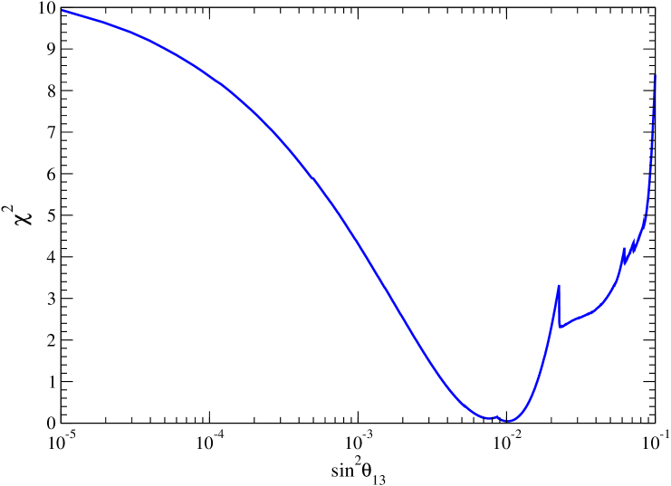
Figure 1: $\chi^{2}$ as a function of the leptonic $\sin^{2}\theta_{13}$ for the normal neutrino mass spectrum.

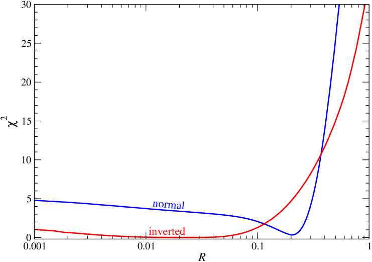
Figure 2: $\chi^{2}$ as a function of $R=m_{\mathrm{min}}/\sqrt{\Delta m^{2}_{\odot}}$, where $m_{\mathrm{min}}=m_{1}$ for the normal and $m_{3}$ for the inverted neutrino mass spectrum.

	$r_{H}$	$r_{F}$	$r_{u}$	$r_{\ell}$	$r_{D}$	$r_{R}$
Normal:	$-71.5516$	$7.16038$	$-2.76118$	$6.57185$	$5842.373$	$1.82618\times 10^{-16}$
Inverted:	$82.0042$	$190.194$	$6.60808$	$-7.22108$	$-43303.97$	$2.22386\times 10^{-18}$

Table 2: The values of the VEV ratios appearing in the mass matrices (25)–(29) obtained in the fits with normal and inverted neutrino mass ordering.

A fit in the case of normal neutrino mass ordering:

We search for a solution in the case of the normal ordering $m_{1}<m_{2}<m_{3}$ of the neutrino masses ($\Delta m^{2}_{\odot}=m_{2}^{2}-m_{1}^{2}$, $\Delta m^{2}_{\mathrm{atm}}=m_{3}^{2}-m_{1}^{2}$). In that case we find an excellent fit with the following properties:

$$\begin{array}[]{l}\chi^{2}=0.33,\quad\sqrt{v_{d}^{2}+v_{u}^{2}}=26.4\>\mbox{GeV},\\[2.84526pt] m_{1}=1.81\times 10^{-3}\>\mbox{eV},\quad m_{2}=0.907\times 10^{-2}\>\mbox{eV},\quad m_{3}=5.006\times 10^{-2}\>\mbox{eV}.\end{array}$$ (33)

In the second relation in this equation we have used $w_{R}=M_{\mathrm{GUT}}$—see Eq. (2). The corresponding values of the matrix elements of $H^{\prime}$, $G^{\prime}$, $F^{\prime}$ are given by

$$H^{\prime} = \left(\begin{array}[]{ccc}0.198268&0&0\\ 0&-0.896317&0\\ 0&0&1150.786\end{array}\right),$$ (37)

$$G^{\prime} = \left(\begin{array}[]{ccc}0&2.68402&1.67616\\ -2.68402&0&-0.580726\\ -1.67616&0.580726&0\end{array}\right),$$ (41)

$$F^{\prime} = \left(\begin{array}[]{ccc}3.23879&5.69390&-10.0743\\ 5.69390&19.1109&-33.5646\\ -10.0743&-33.5646&-44.3762\end{array}\right),$$ (45)

where all numerical values are in units of MeV. The fit values of the VEV ratios are listed in Table 2. The $\chi^{2}$ of the fit practically comes only from two observables: the pull of $\sin^{2}\theta_{13}$ (leptonic mixing angle) is 0.45 and the pull of $m_{b}$ is 0.31.

We can ask the question if our scenario makes some predictions. For the best fit we find $\delta_{\mathrm{PMNS}}=-2.0^{\circ}$. However, this small value misleading, because pinning $\delta_{\mathrm{PMNS}}$ in $\chi^{2}$ shows that in the large range $-60^{\circ}\ \mbox{\raisebox{-3.0pt}{$\stackrel{{\scriptstyle\displaystyle<}}{{\sim}}$}}\ \delta_{\mathrm{PMNS}}\ \mbox{\raisebox{-3.0pt}{$\stackrel{{\scriptstyle\displaystyle<}}{{\sim}}$}}\ 60^{\circ}$ the fit is still very good, with $\chi^{2}\ \mbox{\raisebox{-3.0pt}{$\stackrel{{\scriptstyle\displaystyle<}}{{\sim}}$}}\ 1$. The worst $\chi^{2}$ is about 15 and occurs around $\delta_{\mathrm{PMNS}}\sim 175^{\circ}$, where for instance $m_{b}$ is not well reproduced and the leptonic $\sin^{2}\theta_{13}$ becomes too large. As for $\sin^{2}\theta_{13}$, Fig. 1 shows that the preferred value is about 0.01. However, we cannot consider this as a prediction since in a wide range around this value the $\chi^{2}$ is still acceptable. Only at very small $\sin^{2}\theta_{13}$ the fit becomes bad, mainly because of $m_{d}$, $m_{b}$ and the atmospheric mixing angle $\theta_{23}$. The quantity $R=m_{1}/\sqrt{\Delta m^{2}_{\odot}}$ measures how hierarchical a normal neutrino mass spectrum is. The $\chi^{2}$ as a function of $R$ is depicted in Fig. 2. We read off that $R\sim 0.2$ is preferred and the $\chi^{2}$ quickly becomes bad for larger $R$, mainly owing to $m_{d}$, $m_{b}$ and the leptonic $\sin^{2}\theta_{13}$. Also for very small $R$ the fit worsens, for similar reasons as for large $R$, however, not in a dramatic way. On the other hand, in the MSGUT there is a preferred range $0.2\ \mbox{\raisebox{-3.0pt}{$\stackrel{{\scriptstyle\displaystyle<}}{{\sim}}$}}\ R\ \mbox{\raisebox{-3.0pt}{$\stackrel{{\scriptstyle\displaystyle<}}{{\sim}}$}}\ 2$ and there is a genuine lower bound on $R$ as well [17].

With Eq. (30) and the upper bound on $\sqrt{v_{d}^{2}+v_{u}^{2}}$ in Eq. (33) we see that we are allowed to raise $w_{R}$ to $w_{R}\sim 6\times M_{\mathrm{GUT}}$, without violating the inequality (31).

It has to be checked that our numerical solution given by Eq. (41) and Table 2 respects the perturbative regime in the Yukawa sector. Since the procedure has been explained in detail in [24], we confine ourselves to the essentials. The two Higgs doublets of the MSSM, $H_{d}$ and $H_{u}$, have hypercharges $+1/2$ and $-1/2$ and VEVs $v\cos\beta$ and $v\sin\beta$, respectively. The corresponding Yukawa coupling matrices are given by $Y_{d}=M_{d}/(v\cos\beta)$, etc. It turns out that the largest Yukawa couplings are $\left(Y_{u}\right)_{33}\simeq\left(Y_{D}\right)_{33}$, where the largest contribution comes from $H^{\prime}_{33}$. Using $\tan\beta=10$, it is given by $r_{H}H^{\prime}_{33}/(v\sin\beta)\simeq-0.48$. This confirms that the Yukawa couplings are safely in the perturbative regime.

Finally, we want to estimate the size of type II seesaw contributions to $\mathcal{M}_{\nu}$. The corresponding mass matrix is given by $w_{L}F^{\prime}/v_{d}=w_{L}F^{\prime}/(r_{R}M_{\mathrm{GUT}})$—see Eqs. (2), (21) and (30). The largest element in $F^{\prime}$ is the 33-element. With the value of this element from Eq. (41) and $r_{R}$ from Table 2, the type II mass matrix contributes at most $\left(1.2\times 10^{-2}\right)\times w_{L}$. Since we expect $w_{L}\sim v^{2}/M_{\mathrm{GUT}}\sim 10^{-3}$ eV, we find the announced suppression with respect to type I seesaw contributions.

A fit for the inverted neutrino mass spectrum:

Searching for a fit by imposing the inverted ordering $m_{3}<m_{1}<m_{2}$ of the neutrino masses ($\Delta m^{2}_{\odot}=m_{2}^{2}-m_{1}^{2}$ as for the normal spectrum, but $\Delta m^{2}_{\mathrm{atm}}=m_{2}^{2}-m_{3}^{2}$), we find a solution which is even better as in the case of normal ordering. It has the following properties:

$$\begin{array}[]{l}\chi^{2}=0.011,\quad\sqrt{v_{d}^{2}+v_{u}^{2}}=8.46\>\mbox{GeV},\\[2.84526pt] m_{1}=4.920\times 10^{-2}\>\mbox{eV},\quad m_{2}=5.000\times 10^{-2}\>\mbox{eV},\quad m_{3}=2.18\times 10^{-4}\>\mbox{eV},\end{array}$$ (46)

with the matrices

$$H^{\prime} = \left(\begin{array}[]{ccc}2.39744&0&0\\ 0&33.6387&0\\ 0&0&1127.980\end{array}\right),$$ (50)

$$G^{\prime} = \left(\begin{array}[]{ccc}0&-2.41722&-2.65793\\ 2.41722&0&0.0107775\\ 2.65793&-0.0107775&0\end{array}\right),$$ (54)

$$F^{\prime} = \left(\begin{array}[]{ccc}-1.05201&-0.0960901&0.174940\\ -0.0960901&-14.0343&26.0245\\ 0.174940&26.0245&-52.9848\end{array}\right),$$ (58)

where all numerical values are in units of MeV, and the VEV ratios are displayed in Table 2. For all practical purposes the fit is perfect and there is no need to give any pull values.

Now we come to the predictions of our scenario in the case of the inverted neutrino mass spectrum. Concerning CP violation in neutrino oscillations, our best fit gives $\delta_{\mathrm{PMNS}}=-107.6^{\circ}$. However, this value has no meaning because $\chi^{2}$ as a function of $\delta_{\mathrm{PMNS}}$ is flat for all practical purposes. The same is true for the leptonic quantities $\sin^{2}\theta_{23}$ and $\sin^{2}\theta_{13}$ in the physically relevant ranges. However, there is a definite prediction for the neutrino mass spectrum: hierarchy is strongly preferred—see Fig. 2. When the quantity $R=m_{3}/\sqrt{\Delta m^{2}_{\odot}}$ becomes large the fit turns bad; however, there is no clear-cut reason, it is mostly the down-quark masses and the top-quark mass which are not well reproduced and the fit value of the leptonic $\sin^{2}\theta_{13}$ is around its experimental upper bound.

In the second relation of Eq. (46) we have again used our reference value (2). Now inequality (31) is respected for $w_{R}\ \mbox{\raisebox{-3.0pt}{$\stackrel{{\scriptstyle\displaystyle<}}{{\sim}}$}}\ 20\times M_{\mathrm{GUT}}$, i.e. there is more freedom for $w_{R}$ than in the normal case.

As before, large Yukawa couplings in $Y_{u}$ and $Y_{D}$ are induced by $H^{\prime}_{33}$. But now, because $r_{D}$ is so big, a slightly larger coupling is $\left(Y_{D}\right)_{13}\simeq ir_{D}G^{\prime}_{13}/(v\sin\beta)\simeq i\times 0.66$, still in the perturbative regime. The discussion of the smallness of type II seesaw contributions to $\mathcal{M}_{\nu}$ proceeds as for the normal spectrum.

In Eq. (54) the elements $G^{\prime}_{23}$, $F^{\prime}_{12}$ and $F^{\prime}_{13}$ are rather small. This might suggest to set them zero, which is achieved by the horizontal $\mathbbm{Z}_{2}$ symmetry $\psi_{L1}\to-\psi_{L1}$, $D_{pqr}\to-D_{pqr}$. However, this is untenable because it would lead to vanishing $\delta_{\mathrm{CKM}}$. The reason is that this horizontal $\mathbbm{Z}_{2}$ can be combined with the CP transformation of Section 2 to a new symmetry CP^′, under which the vacuum state of our scenario is invariant. Consequently, in that case there is no CP violation [34, 35] and one can show—as it must be in such a case—that $\exp(i\delta_{\mathrm{CKM}})=\pm 1$ [35].

4 Conclusions

In this paper we have investigated fermion masses and mixings in an SUSY $SO(10)$ scenario, originally proposed in [21], where the Yukawa coupling matrices of the scalars in the irreps $\mathbf{10}$, $\mathbf{120}$ and $\overline{\mathbf{126}}$ are real and CP violation is induced only by imaginary VEVs of the $\mathbf{120}$. This gives a scenario with 18 real parameters in the fermion mass sector. Recent results from the MSGUT require a single heavy $SO(10)$ breaking scale, which is then cogent for the MSGUT extended by the $\mathbf{120}$ as well.

There are the following differences between Ref. [21] and the present paper: Firstly, our $\mathcal{M}_{\nu}$ is induced by the type I seesaw mechanism and type II is negligible, whereas in [21] it was assumed that type II dominates. Secondly, we use a purely numerical method, employing the minimization of a $\chi^{2}$ function, whereas Ref. [21] uses an approximate semianalytical method.

We have found excellent fits to fermion masses and mixings for both types of neutrino mass spectra. We want to emphasize this in particular for the inverted mass spectrum, for which the system of fermion mass matrices in the MSGUT—which has no $\mathbf{120}$—does not allow an acceptable fit [17], though complex Yukawa couplings and VEVs and contributions to $\mathcal{M}_{\nu}$ from both seesaw types are admitted. The fits presented in this paper have the following features. The diagonal Yukawa coupling matrix $H$ of the $\mathbf{10}$ is strongly hierarchical and is responsible, in the charged-fermion mass spectra, for the hierarchy between 2nd and 3rd families. The correct size of the neutrino masses is reproduced by a cooperation of two effects: rather large contributions $r_{H}H+ir_{D}G$ to the neutrino Dirac-mass matrix $M_{D}$ from the couplings of the $\mathbf{10}$ and $\mathbf{120}$, where $G$ is the Yukawa coupling matrix of the $\mathbf{120}$, and a moderately small coupling matrix $F$ of the $\overline{\mathbf{126}}$, which enters with its inverse in the type I seesaw formula. The contribution of the $\mathbf{120}$ to the charged-fermion masses and to the CKM matrix is rather small, whereas $r_{D}G$ in $M_{D}$ introduces large leptonic mixing angles. Similar features were found in the previous sample fit of [24], though the assumptions concerning the fermion mass matrices in that paper are quite different from those in the present paper, apart from the use of spontaneous CP violation in both scenarios.

Unfortunately, our scenario is not very predictive. However, it does have one clear-cut prediction, namely hierarchy for both the normal and inverted neutrino mass spectrum. This is quantified by the observable $R$ in Fig. 2 from where we read off $m_{\mathrm{min}}\ll\sqrt{\Delta m^{2}_{\odot}}$.

Apparently, extending the MSGUT by the $\mathbf{120}$ leads to an ambiguous situation concerning fermion mass matrices: quite different assumptions can result in excellent fits. Whether these fits are compatible with the NMSGUT [27], where the VEVs are subject to certain relations, remains to be checked. One aspect seems to emerge: spontaneous CP violation plays in important role in both the fermion mass matrices [24] and the spontaneous breaking [27] of $SO(10)$.

Acknowledgment: W.G. is grateful to L. Lavoura for useful discussions.

Appendix A The spinor representation of $SO(10)$

A possible representation—on the space $\mathcal{H}$ of the fivefold tensor product of $\mathbbm{C}^{2}$—for the Clifford algebra associated with the Lie algebra $so(10)$ is given by [36]

$$\Gamma_{2j-1}=\sigma_{3}^{(5-j)}\otimes\sigma_{1}\otimes\mathbbm{1}^{(j-1)},\quad\Gamma_{2j}=\sigma_{3}^{(5-j)}\otimes\sigma_{2}\otimes\mathbbm{1}^{(j-1)}\quad(j=1,\ldots,5),$$ (A1)

where a superscript $(k)$ denotes the $k$-fold tensor product. The $2\times 2$ matrices $\sigma_{i}$ ($i=1,2,3$) are the Pauli matrices and $\mathbbm{1}$ denotes the $2\times 2$ unit matrix. It is easy to check that the $\Gamma_{p}$ ($p=1,\ldots,10$) fulfill

$$\{\Gamma_{p},\Gamma_{q}\}=2\delta_{pq}\mathbbm{1}^{(5)}\quad\mbox{and}\quad\quad\Gamma_{p}=\Gamma_{p}^{\dagger}=\Gamma_{p}^{-1}.$$ (A2)

It is well known that the matrices

$${\textstyle\frac{1}{2}}\sigma_{pq}\equiv{\textstyle\frac{1}{2}}\Gamma_{p}\Gamma_{q}\quad 1\leq p<q\leq 10,$$ (A3)

have precisely the same commutation relations as the basis elements

$$(M_{pq})_{jk}=\delta_{pj}\delta_{qk}-\delta_{qj}\delta_{pk},\quad 1\leq p<q\leq N,$$ (A4)

of $so(10)$. The $\sigma_{pq}$ generate the spinor irrep $\mathbf{16}$ of $so(10)$ on the 16-dimensional space

$$\frac{1}{2}\left(\mathbbm{1}^{(5)}+\Gamma_{11}\right)\mathcal{H}\quad\mbox{with}\quad\Gamma_{11}=\sigma_{3}^{(5)}.$$ (A5)

Note that $\Gamma_{11}$ anticommutes with all $\Gamma_{p}$ ($p=1,\ldots,10$).

For the Yukawa couplings one needs the matrix $\mathcal{B}$ and its following properties:

$$\mathcal{B}\equiv\Gamma_{1}\Gamma_{3}\Gamma_{5}\Gamma_{7}\Gamma_{9},\quad\mathcal{B}=\mathcal{B}^{\dagger}=\mathcal{B}^{-1},\quad\Gamma_{p}\mathcal{B}=\xi_{p}\mathcal{B}\Gamma_{p}\quad\mbox{with}\quad\xi=(-1)^{1+p}.$$ (A6)

References

• [1] H. Fritzsch, P. Minkowski, Ann. Phys. 93 (1975) 193.
• [2] P. Minkowski, Phys. Lett. B 67 (1977) 421;
T.Yanagida, in Proceedings of the Workshop on Unified Theory and Baryon Number in the Universe, O. Sawata and A. Sugamoto eds., KEK report 79-18, Tsukuba, Japan, 1979;
S.L. Glashow, in Quarks and Leptons, Proceedings of the Advanced Study Institute (Cargรจse, Corsica, 1979), J.-L. Basdevant et al. eds., Plenum, New York, 1981;
M. Gell-Mann, P. Ramond, and R. Slansky, in Supergravity, D.Z. Freedman and F. van Nieuwenhuizen eds., North Holland, Amsterdam, 1979;
R.N. Mohapatra, G. Senjanoviฤ‡, Phys. Rev. Lett. 44 (1980) 912.
• [3] G. Lazarides, Q. Shafi, C. Wetterich, Nucl. Phys. B 181 (1981) 287;
R.N. Mohapatra, G. Senjanoviฤ‡, Phys. Rev. D 23 (1981) 165;
R.N. Mohapatra, P. Pal, Massive Neutrinos in Physics and Astrophysics, World Scientific, Singapore, 1991, p. 127.
• [4] J. Schechter, J.W.F. Valle, Phys. Rev. D 22 (1980) 2227;
S.M. Bilenky, J. Hoลกek, S.T. Petcov, Phys. Lett. B 94 (1980) 495;
I.Yu. Kobzarev, B.V. Martemyanov, L.B.ย Okun, M.G. Shchepkin, Yad. Phys. 32 (1980) 1590 [Sov. J. Nucl. Phys. 32 (1981) 823];
J. Schechter, J.W.F. Valle, Phys. Rev. D 25 (1982) 774.
• [5] G. Senjanoviฤ‡, in Proceedings of SEESAW25: International conference on the seesaw mechanism and the neutrino mass, 10โ€“11 June 2004, Paris, France, J. Orloff, S. Lavignac, and M. Cribier eds., World Scientific, Singapore, 2005, p.ย 45 [hep-ph/0501244].
• [6] R.N. Mohapatra, B. Sakita, Phys. Rev. D 21 (1980) 1062.
• [7] R. Slansky, Phys. Rept. 79 (1981) 1.
• [8] C.S. Aulakh, R.N. Mohapatra, Phys. Rev. D 28 (1983) 217;
T.E. Clark, T.K. Kuo, N. Nakagawa, Phys. Lett 115B (1982) 26;
K.S. Babu, R.N. Mohapatra, Phys. Rev. Lett. 70 (1993) 2845 [hep-ph/9209215];
C.S. Aulakh, B. Bajc, A. Melfo, G. Senjanoviฤ‡, F. Vissani, Phys. Lett. B 588 (2004) 196 [hep-ph/0306242].
• [9] K. Matsuda, Y. Koide, T. Fukuyama, Phys. Rev. D 64 (2001) 053015 [hep-ph/0010026];
K. Matsuda, Y. Koide, T. Fukuyama, H. Nishiura, Phys. Rev. D 65 (2002) 033008 (Erratum-ibid. D 65 (2002) 079904) [hep-ph/0108202];
T. Fukuyama, N. Okada, JHEP 11 (2002) 011 [hep-ph/0205066];
B. Bajc, G. Senjanoviฤ‡, F. Vissani, Phys. Rev. Lett. 90 (2003) 051802 [hep-ph/0210207];
H.S. Goh, R.N. Mohapatra, S.P. Ng, Phys. Lett. B 570 (2003) 215 [hep-ph/0303055];
H.S. Goh, R.N. Mohapatra, S.P. Ng, Phys. Rev. D 68 (2003) 115008 [hep-ph/0308197];
B. Bajc, G. Senjanoviฤ‡, F. Vissani, Phys. Rev. D 70 (2004) 093002 [hep-ph/0402140].
• [10] K.S. Babu, C. Macesanu, Phys. Rev. D 72 (2005) 115003 [hep-ph/0505200].
• [11] K. Matsuda, T. Fukuyama, H. Nishiura, Phys. Rev. D 61 (2000) 053001 [hep-ph/9906433];
S. Bertolini, M. Frigerio, M. Malinskรฝ, Phys. Rev. D 70 (2004) 095002 [hep-ph/0406117];
S. Bertolini, M. Malinskรฝ, Phys. Rev. D 72 (2005) 055021 [hep-ph/0504241].
• [12] C.S. Aulakh, A. Girdar, Int. J. Mod. Phys. A 20 (2005) 865 [hep-ph/0204097];
T. Fukuyama, A. Ilakovac, T. Kikuchi, S. Meljanac, N. Okada, Eur. Phys. J. C 42 (2005) 191 [hep-ph/0401213];
B. Bajc, A. Melfo, G. Senjanoviฤ‡, F. Vissani, Phys. Rev. D 70 (2004) 035007 [hep-ph/0402122];
C.S. Aulakh, A. Girdar, Nucl. Phys. B 711 (2005) 275 [hep-ph/0405074];
T. Fukuyama, A. Ilakovac, T. Kikuchi, S. Meljanac, N. Okada, J. Math. Phys. 46 (2005) 033505 [hep-ph/0405300];
T. Fukuyama, A. Ilakovac, T. Kikuchi, S. Meljanac, N. Okada, Phys. Rev. D 72 (2005) 051701 [hep-ph/0412348];
C.S. Aulakh, Phys. Rev. D 72 (2005) 051702 [hep-ph/0501025].
• [13] M. Maltoni, T. Schwetz, M.A. Tรณrtola, J.W.F. Valle, New. J. Phys. 6 (2004) 122 [hep-ph/0405172];
G.L. Fogli, E. Lisi, A. Marrone, A. Palazzo, Prog. Part. Nucl. Phys. 57 (2006) 742 [hep-ph/0506083].
• [14] T.ย Schwetz, Phys. Scripta T 127 (2006) 1 [hep-ph/0606060].
• [15] C.S. Aulakh, expanded version of the plenary talks at the Workshop Series on Theoretical High Energy Physics, IIT Roorkee, Uttaranchal, India, March 16โ€“20, 2005, and at the 8th European Meeting โ€œFrom the Planck Scale to the Electroweak Scaleโ€ (PLANCK05), ICTP, Trieste, Italy, May 23โ€“28, 2005, hep-ph/0506291;
B. Bajc, A. Melfo, G. Senjanoviฤ‡, F. Vissani, Phys. Lett. B 634 (2006) 272 [hep-ph/0511352].
• [16] C.S. Aulakh, S.K. Garg, Nucl. Phys. B 757 (2006) 47 [hep-ph/0512224].
• [17] S. Bertolini, T. Schwetz, M. Malinskรฝ, Phys. Rev. D 73 (2006) 115012 [hep-ph/0605006].
• [18] C.S. Aulakh, hep-ph/0602132.
• [19] N. Oshimo, Phys. Rev. D 66 (2002) 0950 [hep-ph/0206239];
N. Oshimo, Nucl. Phys. B 668 (2003) 258 [hep-ph/0305166].
• [20] Wei-Min Yang, Zhi-Gang Wang, Nucl. Phys. 707 (2005) 87 [hep-ph/0406221].
• [21] B. Dutta, Y. Mimura, R.N. Mohapatra, Phys. Lett. B 603 (2004) 35 [hep-ph/0406262].
• [22] B. Dutta, Y. Mimura, R.N. Mohapatra, Phys. Rev. Lett. 94 (2005) 091804 [hep-ph/0412105];
B. Dutta, Y. Mimura, R.N. Mohapatra, Phys. Rev. D 72 (2005) 075009 [hep-ph/0507319].
• [23] L. Lavoura, H. Kรผhbรถck, W. Grimus, Nucl. Phys. B 754 (2006) 1 [hep-ph/0603259].
• [24] W. Grimus, H. Kรผhbรถck, hep-ph/0607197, to be published in Phys. Lett. B.
• [25] C.S. Aulakh, hep-ph/0607252;
C.S. Aulakh, talk presented at 33rd International Conference on High Energy Physics (ICHEP06), Moscow, Russia, July 26โ€“August 2, 2006, hep-ph/0610097.
• [26] J.C. Pati, A. Salam, Phys. Rev. D 8 (1973) 1240.
• [27] C.S. Aulakh, S.K. Garg, hep-ph/0612021.
• [28] N.V. Smolyakov, Theor. and Math. Phys. 50 (1982) 225.
• [29] W. Grimus, M.N. Rebelo, Phys. Rept. 281 (1997) 239 [hep-ph/9506272].
• [30] D. Chang, R.N. Mohapatra, M.K. Parida, Phys. Rev. Lett. 52 (1984) 1072;
D. Chang, R.N. Mohapatra, M.K. Parida, Phys. Rev. D 30 (1984) 1052.
• [31] C.R. Das, M.K. Parida, Eur. Phys. J. C 20 (2001) 121 [hep-ph/0010004].
• [32] W.-M. Yao et al., Review of Particle Physics, J. Phys. G 33 (2006) 1.
• [33] J.A. Nelder, R. Mead, Comp. J. 7 (1965) 306;
W.H. Press, B.P. Flannery, S.A. Teukolsky, W.T. Vetterling, Numerical recipes in C: The art of scientific computing, Cambridge University Press, 1992.
• [34] G.C. Branco, J.-M. Gรฉrard, W. Grimus, Phys. Lett. B 136 (1984) 383.
• [35] G. Ecker, W. Grimus, H. Neufeld, Nucl. Phys. B 247 (1984) 70.
• [36] F. Wilczek, A. Zee, Phys. Rev. D 25 (1982) 553.