Abstract

We give a brief introduction to chiral perturbation theory in its various settings. We discuss some applications of recent interest including chiral extrapolations for lattice gauge theory.

Commissioned article for Ann. Rev. Nucl. Part. Sci.

1 Introduction and disclaimer

Quantum chromodynamics (QCD) is the theory of the strong interactions. While asymptotic freedom allows for a perturbative analysis at large energies, the low energy domain is characterized by the appearance of hadrons that contain (and hide) the fundamental QCD degrees of freedom – the quarks and gluons. This property of QCD is called confinement, it is beyond the reach of perturbation theory, calling for a non-perturbative treatment. Furthermore, QCD also exhibits spontaneous, explicit and anomalous symmetry breaking – and exactly the consequences of these broken symmetries can be analyzed in terms of an appropriately formulated effective field theory (EFT). This EFT is chiral perturbation theory (CHPT) and in the following we will review its salient properties together with some phenomenological applications and the connection to the lattice formulation of QCD. Lattice QCD promises exact solutions utilizing a formulation on a discretized space-time and solving the pertinent path integral with the help of large computers. Most lattice calculations are, however, done at unphysically large quark masses – and chiral perturbation theory offers a model-independent scheme to perform the necessary chiral extrapolations.

We end this introduction with a disclaimer: This is not an all purpose review but rather stresses some fundamentals and selected applications. In what follows, we supply a sufficient amount of references for the reader to immerse deeper into the subject.

The manuscript is organized as follows. In Sec. 2 we discuss the symmetries of QCD and their realization underlying the effective field theory. The corresponding effective Lagrangian and the pertinent power counting are given in Sec. 3, while Sec. 4 contains some remarks on chiral loops and the meaning of the low–energy coupling constants of the EFT. As a specific example, the scalar form factor of the pion is analyzed to one loop accuracy in Sec. 5. The role of unitarity and analyticity is discussed in Sec. 6, in particular, we discuss the dispersive representation of the scalar pion form factor and show how dispersion relations and CHPT can be combined to give accurate predictions of low-energy observables. A few selected applications that represent the state-of-the-art in CHPT and a discussion of the interplay between lattice QCD (LQCD) and CHPT are given in Sec. 7.

2 QCD symmetries and their realization

First, we must discuss chiral symmetry in the context of QCD. Chromodynamics is a non-abelian $SU(3)_{\rm color}$ gauge theory with $N_{f}$ flavors of quarks, three of them being light ($u,d,s$) and the other three heavy ($c,b,t$). Here, light and heavy refers to a typical hadronic scale of about 1 GeV. In what follows, we consider light quarks only (the heavy quarks are to be considered as decoupled). The QCD Lagrangian reads

$${\mathcal{L}}_{\rm QCD}=-\frac{1}{2g^{2}}{\rm Tr}\left(G_{\mu\nu}G^{\mu\nu}\right)+\bar{q}\,i\gamma^{\mu}D_{\mu}\,q-\bar{q}{\mathcal{M}}\,q={\mathcal{L}}_{\rm QCD}^{0}-\bar{q}{\mathcal{M}}\,q~{},$$ (1)

where we have absorbed the gauge coupling in the definition of the gluon field and color indices are suppressed. The three-component vector $q$ collects the quark fields, $q^{T}(x)=\left(u(s),d(x),s(x)\right)$. As far as the strong interactions are concerned, the different quarks $u,d,s$ have identical properties, except for their masses. The quark masses are free parameters in QCD - the theory can be formulated for any value of the quark masses. In fact, light quark QCD can be well approximated by a fictitious world of massless quarks, denoted ${\mathcal{L}}_{\rm QCD}^{0}$ in Eq. (1). Remarkably, this theory contains no adjustable parameter - the gauge coupling $g$ merely sets the scale for the renormalization group invariant scale $\Lambda_{\rm QCD}$. Furthermore, in the massless world left- and right-handed quarks are completely decoupled. These are defined via

$$q_{L}=P_{L}\,q~{},\quad q_{R}=P_{R}\,q~{},$$ (2)

in terms of the projection operators

$$P_{L} = \frac{1}{2}(1+\gamma_{5})~{},~{}~{}P_{R}=\frac{1}{2}(1-\gamma_{5})~{},$$

$$P_{L}^{2} = P_{L}~{},~{}~{}P_{R}^{2}=P_{R}~{},~{}~{}P_{L}+P_{R}={\bf 1}~{},~{}~{}P_{L}\cdot P_{R}=0~{}.$$ (3)

The Lagrangian of massless QCD is invariant under separate unitary global transformations of the left- and right-hand quark fields, the so-called chiral rotations,

$$q_{I}\to V_{I}q_{I}~{},\quad V_{I}\in U(3)~{},\quad I=L,R~{},$$ (4)

leading to $3^{2}=9$ conserved left- and $9$ conserved right-handed currents by virtue of Noether’s theorem. These can be expressed in terms of vector ($V\sim L+R$) and axial-vector ($A\sim L-R$) currents

$$V_{0}^{\mu} = \bar{q}\,\gamma^{\mu}\,q~{},\quad V_{\mu}^{a}=\bar{q}\,\gamma^{\mu}\frac{\lambda_{a}}{2}\,q~{},$$

$$A_{0}^{\mu} = \bar{q}\,\gamma^{\mu}\gamma_{5}\,q~{},\quad A_{\mu}^{a}=\bar{q}\,\gamma^{\mu}\gamma_{5}\frac{\lambda_{a}}{2}\,q~{},$$ (5)

Here, $a=1,\ldots 8$, and the $\lambda_{a}$ are Gell-Mann’s $SU(3)$ flavor matrices. As discussed later, the singlet axial current is anomalous, and thus not conserved. The actual symmetry group of massless QCD is generated by the charges of the conserved currents, it is $G_{0}=SU(3)_{R}\times SU(3)_{L}\times U(1)_{V}$. The $U(1)_{V}$ subgroup of $G_{0}$ generates conserved baryon number since the isosinglet vector current counts the number of quarks minus antiquarks in a hadron. The remaining group $SU(3)_{R}\times SU(3)_{L}$ is often referred to as chiral $SU(3)$. Note that one also considers the light $u$ and $d$ quarks only (with the strange quark mass fixed at its physical value), in that case, one speaks of chiral $SU(2)$ and must replace the generators in Eq. (2) by the Pauli-matrices. Let us mention that QCD is also invariant under the discrete symmetries of parity ($P$), charge conjugation ($C$) and time reversal ($T$). Although interesting in itself, we do not consider strong $CP$ violation and the related $\theta$-term in what follows, see e.g. [1].

The chiral symmetry is a symmetry of the Lagrangian of QCD but not of the ground state or the particle spectrum – to describe the strong interactions in nature, it is crucial that chiral symmetry is spontaneously broken. This can be most easily seen from the fact that hadrons do not appear in parity doublets. If chiral symmetry were exact, from any hadron one could generate by virtue of an axial transformation another state of exactly the same quantum numbers except of opposite parity. The spontaneous symmetry breaking leads to the formation of a quark condensate in the vacuum $\sim\langle 0|\bar{q}q|0\rangle=\langle 0|\bar{q}_{L}q_{R}+\bar{q}_{R}q_{L}|0\rangle$, thus connecting the left- with the right-handed quarks. In the absence of quark masses this expectation value is flavor-independent: $\langle 0|\bar{u}u|0\rangle=\langle 0|\bar{d}d|0\rangle=\langle 0|\bar{q}q|0\rangle$. More precisely, the vacuum is only invariant under the subgroup of vector rotations times the baryon number current, $H_{0}=SU(3)_{V}\times U(1)_{V}$. This is the generally accepted picture that is supported by general arguments [2] as well as lattice simulations of QCD (for a recent study, see [3] and references therein). In fact, the vacuum expectation value of the quark condensate is only one of the many possible order parameters characterizing the spontaneous symmetry violation - all operators that share the invariance properties of the vacuum (Lorentz invariance, parity, invariance under $SU(3)_{V}$ transformations) qualify as order parameters. The quark condensate nevertheless enjoys a special role, it can be shown to be related to the density of small eigenvalues of the QCD Dirac operator (see [4] and more recent discussions in [5, 6]),

$$\lim_{{\cal M}\to 0}\langle 0|\bar{q}q|0\rangle=-\pi\,\rho(0)~{}.$$ (6)

For free fields, $\rho(\lambda)\sim\lambda^{3}$ near $\lambda=0$. Only if the eigenvalues accumulate near zero, one obtains a non-vanishing condensate. This scenario is indeed supported by lattice simulations and many model studies involving topological objects like instantons or monopoles.

Before discussing the implications of spontaneous symmetry breaking for QCD, we briefly remind the reader of Goldstone’s theorem [7, 8]: to every generator of a spontaneously broken symmetry corresponds a massless excitation of the vacuum. This can be understood in a nut-shell (ignoring subtleties like the normalization of states and alike - the argument also goes through in a more rigorous formulation). Be ${\cal H}$ some Hamiltonian that is invariant under some charges $Q^{i}$, i.e. $[{\cal H},Q^{i}]=0$ with $i=1,\ldots,n$. Assume further that $m$ of these charges ($m\leq n$) do not annihilate the vacuum, that is $Q^{j}|0\rangle\neq 0$ for $j=1,\ldots,m$. Define a single-particle state via $|\psi\rangle=Q^{j}|0\rangle$. This is an energy eigenstate with eigenvalue zero, since $H|\psi\rangle=HQ^{j}|0\rangle=Q^{j}H|0\rangle=0$. Thus, $|\psi\rangle$ is a single-particle state with $E=\vec{p}=0$, i.e. a massless excitation of the vacuum. These states are the Goldstone bosons, collectively denoted as pions $\pi(x)$ in what follows. Through the corresponding symmetry current the Goldstone bosons couple directly to the vacuum,

$$\langle 0|J^{0}(0)|\pi\rangle\neq 0~{}.$$ (7)

In fact, the non-vanishing of this matrix element is a necessary and sufficient condition for spontaneous symmetry breaking. In QCD, we have eight (three) Goldstone bosons for $SU(3)$ ($SU(2)$) with spin zero and negative parity – the latter property is a consequence that these Goldstone bosons are generated by applying the axial charges on the vacuum. The dimensionful scale associated with the matrix element Eq. (7) is the pion decay constant (in the chiral limit)

$$\langle 0|A^{a}_{\mu}(0)|\pi^{b}(p)\rangle=i\delta^{ab}Fp_{\mu}~{},$$ (8)

which is a fundamental mass scale of low-energy QCD. In the world of massless quarks, the value of $F$ differs from the physical value by terms proportional to the quark masses, to be introduced later, $F_{\pi}=F[1+{\cal O}({\cal M})]$. The physical value of $F_{\pi}$ is $92.4\,$MeV, determined from pion decay, $\pi\to\nu\mu$. For a discussion of $F_{\pi}$ in the context of the SM and beyond, see [9].

Of course, in QCD the quark masses are not exactly zero. The quark mass term leads to the so-called explicit chiral symmetry breaking. Consequently, the vector and axial-vector currents are no longer conserved (with the exception of the baryon number current)

$$\partial_{\mu}V_{a}^{\mu}=\displaystyle\frac{1}{2}i\bar{q}\,[{\cal M},\lambda_{a}]\,q~{},\quad\partial_{\mu}A_{a}^{\mu}=\displaystyle\frac{1}{2}i\bar{q}\,\{{\cal M},\lambda_{a}\}\,\gamma_{5}\,q~{}.$$ (9)

However, the consequences of the spontaneous symmetry violation can still be analyzed systematically because the quark masses are small. QCD possesses what is called an approximate chiral symmetry. In that case, the mass spectrum of the unperturbed Hamiltonian and the one including the quark masses can not be significantly different. Stated differently, the effects of the explicit symmetry breaking can be analysed in perturbation theory. This perturbation generates the remarkable mass gap of the theory - the pions (and, to a lesser extent, the kaons and the eta) are much lighter than all other hadrons. To be more specific, consider chiral $SU(2)$. The second formula of Eq. (9) is nothing but a Ward-identity (WI) that relates the axial current $A^{\mu}=\bar{d}\gamma^{\mu}\gamma_{5}u$ with the pseudoscalar density $P=\bar{d}i\gamma_{5}u$,

$$\partial_{\mu}A^{\mu}=(m_{u}+m_{d})\,P~{}.$$ (10)

Taking on-shell pion matrix elements of this WI, one arrives at

$$M_{\pi}^{2}=(m_{u}+m_{d})\frac{G_{\pi}}{F_{\pi}}~{},$$ (11)

where the coupling $G_{\pi}$ is given by $\langle 0|P(0)|\pi(p)\rangle=G_{\pi}$. This equation leads to some intriguing consequences: In the chiral limit, the pion mass is exactly zero - in accordance with Goldstone’s theorem. More precisely, the ratio $G_{\pi}/F_{\pi}$ is a constant in the chiral limit and the pion mass grows as $\sqrt{(}m_{u}+m_{d})$ as the quark masses are turned on. A more detailed discussion of the Goldstone boson masses and their relation to the quark masses will be given in Section 7.1.

There is even further symmetry related to the quark mass term. It is observed that hadrons appear in isospin multiplets, characterized by very tiny splittings of the order of a few MeV. These are generated by the small quark mass difference $m_{u}-m_{d}$ (small with respect to the typical hadronic mass scale of a few hundred MeV) and also by electromagnetic effects of the same size (with the notable exception of the charged to neutral pion mass difference that is almost entirely of electromagnetic origin). This can be made more precise: For $m_{u}=m_{d}$, QCD is invariant under $SU(2)$ isospin transformations:

$$q\to q^{\prime}=Uq~{},~{}~{}q=\left(\begin{array}[]{cc}u\\ d\end{array}\right)~{},~{}~{}~{}U=\left(\begin{array}[]{cc}a^{*}&b^{*}\\ -b&a\end{array}\right)~{},~{}~{}~{}|a|^{2}+|b|^{2}=1~{}.$$ (12)

In this limit, up and down quarks can not be disentangled as far as the strong interactions are concerned. Rewriting of the QCD quark mass term allows to make the strong isospin violation explicit:

$${\cal H}_{\rm QCD}^{\rm SB}=m_{u}\,\bar{u}u+m_{d}\,\bar{d}d=\displaystyle\frac{1}{2}(m_{u}+m_{d})(\bar{u}u+\bar{d}d)+\displaystyle\frac{1}{2}(m_{u}-m_{d})(\bar{u}u-\bar{d}d)~{},$$ (13)

where the first (second) term is an isoscalar (isovector). Extending these considerations to $SU(3)$, one arrives at the eighfold way of Gell-Mann and Ne’eman [10] that played a decisive role in our understanding of the quark structure of the hadrons. The $SU(3)$ flavor symmetry is also an approximate one, but the breaking is much stronger than it is the case for isospin. From this, one can directly infer that the quark mass difference $m_{s}-m_{d}$ must be much bigger than $m_{d}-m_{u}$. Again, this will be made more precise in Section 7.1.

There is one further source of symmetry breaking, which is best understood in terms of the path integral representation of QCD. The effective action contains an integral over the quark fields that can be expressed in terms of the so-called fermion determinant. Invariance of the action under chiral transformations not only requires the action to be left invariant, but also the fermion measure [11]. Symbolically,

$$\int[d\bar{q}][dq]\ldots\to|{\mathcal{J}}|\int[d\bar{q}^{\prime}][dq^{\prime}]\ldots$$ (14)

If the Jacobian is not equal to one, $|{\mathcal{J}}|\neq 1$, one encounters an anomaly. Of course, such a statement has to be made more precise since the path integral requires regularization and renormalization, still it captures the essence of the chiral anomalies of QCD. One can show in general that certain 3-, 4-, and 5-point functions with an odd number of external axial-vector sources are anomalous. As particular examples we mention the famous triangle anomalies of Adler, Bell and Jackiw and the divergence of the singlet axial current,

$$\partial_{\mu}(\bar{q}\gamma^{\mu}\gamma_{5}q)=2iqm\gamma_{5}q+\frac{N_{f}}{8\pi}G_{\mu\mu}^{a}\tilde{G}^{\mu\mu,a}~{},$$ (15)

that is related to the generation of the $\eta^{\prime}$ mass. There are many interesting aspects of anomalies in the context of QCD and chiral perturbation theory. Space does not allow to discuss these, we refer to [13].

We end this section by giving list of reviews on the foundations and applications of CHPT, see [12, 13, 14, 15, 16, 17, 18, 19, 20, 21, 22] and a recent status report is Ref. [23]. The state-of-the-art two–loop calculations are reviewed in Ref. [24].

3 Effective chiral Lagrangian and power counting

The appropriate work-horse to analyze the consequences of the spontaneous, the explicit and the anomalous symmetry breaking in QCD is the chiral effective Lagrangian [25]. The relevant degrees of freedom are the Goldstone bosons coupled to external fields. Two remarks are in order: i) extensions of this scheme to include e.g. matter fields are briefly discussed below, and ii) one can equally well work with the generating functional, see e.g. the classical papers [26, 27]. In the chiral limit, we are dealing with a theory without mass gap. Consequently, S-matrix elements and transition currents are dominated by pion-exchange contributions. The QCD Lagrangian can thus be mapped onto an effective Lagrangian,

$${\mathcal{L}}_{\rm QCD}[\bar{q},q,G]\to{\mathcal{L}}_{\rm eff}[U,\partial_{\mu}U,\ldots,{\mathcal{M}}]~{},$$ (16)

where $U(x)$ is a matrix-valued $SU(3)$ field that collects the Goldstone bosons. Further, $\partial_{\mu}U$ reminds us that all interactions are of derivative nature due to Goldstone’s theorem and ${\mathcal{M}}$ keeps track of the explicit symmetry breaking due to the finite quark masses. A formal proof of this equivalence based on the analysis of the chiral Ward identities has been given by Leutwyler [28] and by Weinberg [29] — space does not allow to discuss these beautiful papers in more detail here. The effective Lagrangian leads to a well defined quantum field theory in which gauge and chiral symmetries as well as the chiral anomaly are manifest. The best strategy to construct the most general ${\cal L}_{\rm eff}$ consistent with the QCD symmetries is to consider QCD in the presence of locally chiral invariant external fields,

$${\mathcal{L}}_{\rm QCD} = {\mathcal{L}}_{\rm QCD}^{0}-\bar{q}\,\gamma_{\mu}(v^{\mu}+\gamma_{5}a^{\mu})\,q+\bar{q}\,(s-i\gamma_{5}p)\,q~{},$$ (17)

$$= {\mathcal{L}}_{\rm QCD}^{0}-\bar{q}_{L}\,\gamma_{\mu}P_{L}l^{\mu}\,q_{L}-\bar{q}_{R}\,\gamma_{\mu}P_{R}r^{\mu}\,q_{R}+\ldots$$

in terms of scalar $s(x)$, pseudoscalar $p(x)$, vector $v^{\mu}(x)$ and axial–vector $a^{\mu}(x)$ sources. Explicit symmetry breaking is included in the scalar source, $s(x)={\mathcal{M}}+\ldots={\rm diag}(m_{u}.m_{d},m_{s})+\ldots$. Electroweak interactions are easily incorporated via

$$r_{\mu} = e\,Q\,{\cal A}_{\mu}~{},~{}~{}l_{\mu}=e\,Q\,{\cal A}_{\mu}+\frac{e}{\sqrt{2}\sin^{2}\theta_{W}}\left(W_{\mu}^{+}T_{+}+{\rm h.c.}\right)~{},$$

$$Q = {\rm diag}\left(\displaystyle\frac{2}{3},-\displaystyle\frac{1}{3},-\displaystyle\frac{1}{3}\right)~{},~{}~{}T_{+}=\left(\begin{array}[]{ccc}0&V_{ud}&V_{us}\\ 0&0&0\\ 0&0&0\end{array}\right)~{},$$ (21)

with ${\cal A}_{\mu}$ the photon field, $W_{\mu}$ is the charged massive vector boson field, $\theta_{W}$ the weak mixing angle and $V_{ud},V_{us}$ are the pertinent elements of the CKM matrix. The most important ingredient to make the effective field theory a useful tool is the power counting. In CHPT, we have a dual expansion in small external momenta and small quark masses (with a fixed ratio to have a well defined chiral limit). The corresponding small parameter is denoted by $q$, where small refers to the typical hadronic scale of about 1 GeV. First, one assigns a chiral dimension to all building blocks of ${\mathcal{L}}_{\rm eff}$: $U(x)={\cal O}(1)$, $\partial_{\mu}U(x),l_{\mu}(x),r_{\mu}(x)={\cal O}(q)$ and $s(x),p(x)={\cal O}(q^{2})$. The last assignment is a consequence of Eq. (11) — the Goldstone boson masses are non–analytic in the quark masses. (For an alternative power counting, see [30]). The lowest order effective Lagrangian then takes the form

$${\mathcal{L}}^{(2)}=\frac{F^{2}}{4}\langle D_{\mu}UD^{\mu}U^{\dagger}+\chi U^{\dagger}+\chi^{\dagger}U\rangle~{},$$ (22)

where the brackets denote the trace in flavor space, $D_{\mu}U=\partial_{\mu}U+il_{\mu}U-iUr_{\mu}$ is the chiral covariant derivative and $\chi=2B(s+ip)$ parameterizes the explicit chiral symmetry breaking. The Lagrangian Eq. (22) is consistent with the strictures from Goldstone’s theorem. To this order, the theory is completely specified by two parameters, the pion decay constant in the chiral limit $F$, cf. Eq. (8), and $B$ measures the strength of the quark condensate in the chiral limit, $B=|\langle 0|\bar{q}q|0\rangle|/F^{2}$. At next-to-leading order ${\cal O}(q^{4})$, the effective Lagrangian contains 10 (7) local operators for $SU(3)\,(SU(2))$. These are accompanied by coupling constants not determined by chiral symmetry, the so-called low-energy constants (LECs). For the explicit form of ${\mathcal{L}}^{(4)}$, see [26, 27]. However, at this order there are further contributions. Interactions generate loops, e.g. closing two external lines in a tree-level pion-pion scattering graph leads to the one-loop pion tadpole (pion mass shift) and the chiral anomaly is formally of order $q^{4}$. At two loop order, one has further contributions from tree graphs with dimension six insertions, from one-loop graphs with exactly one insertion from ${\cal L}^{(4)}$ and two–loop graphs with insertions from ${\cal L}^{(2)}$. The complete structure of the effective Lagrangian at two loop order is given in Ref. [31] (where one can also find references to earlier work on that topic). All this is captured in the power counting formula of Weinberg [25], which orders the various contributions to any S–matrix element for pion interactions according to the chiral dimension $D$ (the inclusion of external fields is straightforward),

$$D=2+\sum_{d}N_{d}(d-2)+2L~{},$$ (23)

with $N_{d}$ the number of vertices with dimension $d$ (derivatives and/or pion mass insertions) and $L$ the number of pion loops. Chiral symmetry gives a lower bound for $D$, $D\geq 2$ – these are exactly the tree graphs with lowest order $d=2$ vertices and $L=0$ (giving the soft-pion (current algebra) predictions of the sixties).

To address issues like isospin violation or the extraction of quark mass ratios, one must include virtual photons and leptons in the EFT. Space forbids to discuss the many interesting aspects of these extensions, the interested reader might consult some of the classics, see Refs. [32, 33, 34, 35, 36, 37].

Matter fields like e.g. nucleons can also be included in chiral perturbation theory. In that case, special care has to be taken of the new (hard) mass scale introduced by the matter field (such as the nucleon mass in the chiral limit). This can be treated in various ways for baryons (heavy fermion approach, infrared regularization, extended on-mass-shell scheme and so on). A detailed review on this topic is Ref. [17] and more recent updates can be found in Refs. [38, 39, 40]. Virtual photons in baryon CHPT are addressed e.g. in Refs.[41, 42].

4 Chiral loops and low-energy constants

Beyond tree level, any observable calculated in CHPT receives contributions from tree and and loop graphs. The loops not only generate the imaginary parts but are also – in most cases – divergent requiring regularization and renormalization. In CHPT, one usually chooses a mass–independent regularization scheme to avoid power divergences (there are, however, instances where other regulators are more appropriate or physically intuitive. For a beautiful discussion of this and related issues, see e.g. Refs. [43, 44]). The method of choice in CHPT is dimensional regularization (DR), which introduces the scale $\lambda$. Varying this scale has no influence on any observable $O$ (renormalization scale invariance),

$$\frac{d}{d\lambda}\,O(\lambda)=0~{},$$ (24)

but this also means that it makes little sense to assign a physical meaning to the separate contributions from the contact terms and the loops. Physics, however, dictates the range of scales appropriate for the process under consideration — describing the pion vector radius (at one loop) by chiral loops alone would necessitate a scale of about 1/2 TeV (as stressed long ago by Leutwyler). In this case, the coupling of the $\rho$–meson generates the strength of the corresponding one-loop counterterm that gives most of the pion radius — more on this below. The most intriguing aspects of chiral loops are the so-called chiral logarithms (chiral logs). In the chiral limit, the pion cloud becomes long-ranged and there is no more Yukawa factor $\sim\exp(-M_{\pi}r)$ to cut it off. This generates terms like $\log M^{2}_{\pi},1/M_{\pi},\ldots$, that is contributions that are non–analytic in the quark masses. Such statements can be applied to all hadrons that are surrounded by a cloud of pions which by virtue of their small masses can move away very far from the object that generates them. Stated differently, in QCD the approach to the chiral limit is non–analytic in the quark masses and the low–energy structure of QCD can therefore not be analyzed in terms of a simple Taylor expansion. (An early paper that deals with the subtleties of approaching the chiral limit in QCD is Ref. [45] and literature quoted therein). The exchange of the massless Goldstone bosons generates poles and cuts starting at zero momentum transfer, such that the Taylor series expansion in powers of the momenta fails. This is a general phenomenon of theories that contain massless particles – the Coulomb scattering amplitude due to photon exchange is proportional to $e^{2}/t$, with $t=(p^{\prime}-p)^{2}$ the momentum transfer squared between the two charged particles.

As stated before, most loops are divergent. In DR, all one–loop divergences are simple poles in $1/(d-4)$, where $d$ is the number of space-time dimensions (for renormalization at two loops, see e.g. Ref. [46]). Consequently, these divergences can be absorbed in the pertinent LECs,

$$L_{i}\to L_{i}^{\rm ren}+\beta_{i}\,{\rm L}(\lambda)~{},~{}~{}{\rm L}(\lambda)=\frac{\lambda^{d-4}}{16\pi^{2}}\left(\displaystyle\frac{1}{d-4}-\frac{1}{2}\left(\ln(4\pi)+\Gamma^{\prime}(1)+1\right)\right)~{},$$ (25)

with $\beta_{i}$ the corresponding $\beta$–function and the renormalized and finite $L_{i}^{\rm ren}$ must be determined by a fit to data (or calculated eventually using lattice QCD). Having determined the values of the LECs from experiment, one is faced with the issue of trying to understand these numbers? Not surprisingly, the higher mass states of QCD leave their imprint in the LECs. Consider again the $\rho$-meson contribution to the vector radius of the pion. Expanding the $\rho$-propagator in powers of $t/M_{\rho}^{2}$, its first term is a contact term of dimension four, with the corresponding finite LEC $L_{9}$ given by $L_{9}=F_{\pi}^{2}/2M_{\rho}^{2}\simeq 7.2\cdot 10^{-3}$, close to the empirical value $L_{9}=6.9\cdot 10^{-3}$ at $\lambda=M_{\rho}$. This so–called resonance saturation (pioneered in Refs.[47, 48, 49]) holds more generally for most LECs at one loop and is frequently used in two–loops calculations to estimate the ${\cal O}(p^{6})$ LECs (for a recent study on this issue, see [50]). More precisely, there are two types of LECs — the so-called dynamical LECs and the symmetry breakers. The contributions proportional to the LECs of the first type are non–vanishing in the chiral limit and can be determined from phenomenology. The symmetry breakers, however, are much more difficult to pin down from data and are also difficult to model. Here, recent progress in lattice QCD promises a determination of the contribution from these LECs at unphysical values of the quark masses. Much progress has been made in the field of resonance saturation in the last years, for a state-of-the-art calculation see [51] (and the many references therein). For extensions of the idea of resonance saturation of the LECs in the pion–nucleon and the two–nucleon sectors, see e.g. Refs. [52, 53].

Let us end this section with a short remark on the pion cloud of the nucleon, a topic that has gained some prominence in recent years - the literature abounds with incorrect statements. Consider as an example the isovector Dirac radius of the proton [54]. At third order in the chiral expansion, it takes the form

$$\langle r^{2}\rangle_{1}^{V}=\left(0.61-\left(0.47\,{\rm GeV}^{-2}\right)\tilde{d}(\lambda)+0.47\log\frac{\lambda}{1\,{\rm GeV}}\right)~{}{\rm fm}^{2}~{},$$ (26)

where $\tilde{d}(\lambda)$ is a dimension three pion–nucleon LEC that parameterizes the “nucleon core” contribution. Comparing Eq. (26) with the empirical value for the Dirac radius, $\langle r^{2}\rangle_{1}^{V}=(0.585\,{\rm fm})^{2}$, one finds that even the sign of the core contribution $\sim\tilde{d}(\lambda)$ is not fixed if $\lambda$ is varied within the sensible range from 600 MeV to 1 GeV. Only the sum of the core and the cloud contribution constitutes a meaningful quantity that should be discussed.

5 A specific one–loop calculation

Let us now consider a specific example of a one–loop calculation based on Feynman diagrams – the scalar form factor of the pion (the same calculation using the generating functional can be found in the classical paper [26]). We consider this simple 3-point function because it allows to make our arguments with the least amount of algebra. In chiral $SU(2)$, the coupling of the pion to a scalar-isoscalar source defines the scalar form factor $F_{S}(t)$,

$$\delta^{ik}\,F_{S}(t)=\langle\pi^{i}(p^{\prime})|\bar{q}q|\pi^{k}(p)\rangle~{},\quad t=(p^{\prime}-p)^{2}~{},$$ (27)

with $i,k$ isospin indices and $t$ the invariant four-momentum transfer squared. Since there are no scalar–isoscalar sources, this form factor can only be indirectly inferred making use e.g. of dispersive techniques (see Sec. 6 or Ref. [56]). The important role of the scalar form factor stems from the observation that its value at $t=0$ is proportional to the expectation value of the quark mass term in the QCD Hamiltonian,

$$\frac{\partial M_{\pi}^{2}}{\partial\hat{m}}=\langle\pi|\bar{q}q|\pi\rangle~{}.$$ (28)

To one–loop accuracy, one finds (the pertinent tree and one–loop graphs are shown in Fig. 1)

Figure 1: Graphs contributing to the pion scalar form factor at one loop. The double line denotes the scalar–isoscalar source, solid lines are pions. The filled circle depicts an insertion from the next-to-leading order effective Lagrangian.

$$f(t) = 1+h(t)+{\mathcal{O}}(p^{4})~{},$$

$$h(t) = h_{0}+h_{1}\,t+\frac{1}{2F_{\pi}^{2}}\,\left(2t-M_{\pi}^{2}\right)\,\bar{J}(t)~{}.$$ (29)

Here, $f(t)=F_{S}(t)/2B$ is the normalized scalar form factor and

$$\bar{J}(t)=\frac{1}{16\pi^{2}}\left(\sigma\ln\frac{\sigma-1}{\sigma+1}+2\right)~{},\quad\sigma=\sqrt{1-\frac{4M_{\pi}^{2}}{t}}~{}~{}~{}~{}~{}~{}(t<0)~{},$$ (30)

is the fundamental meson loop-integral (the so-called fundamental bubble) and $h_{0}$ and $h_{1}$ are polynoms in the pion mass (modulo logs) that depend on the one–loop renormalized LECs $\ell_{3}$ and $\ell_{4}$,

$$h_{0} = \frac{M_{\pi}^{2}}{16\pi^{2}F_{\pi}^{2}}\,\left(\ln\frac{M_{\pi}^{2}}{\mu^{2}}+64\pi^{2}\,\ell_{3}(\mu)+\frac{1}{2}\right)~{},$$

$$h_{1} = \frac{1}{16\pi^{2}F_{\pi}^{2}}\,\left(-\ln\frac{M_{\pi}^{2}}{\mu^{2}}+16\pi^{2}\,\ell_{4}(\mu)-1\right)~{}.$$ (31)

These LECs are universal and relate various Green functions. For the case at hand, $\ell_{4}$ can be obtained from the ratio $F_{K}/F_{\pi}$ (extending the theory to $SU(3)$ and then matching the corresponding LEC to $\ell_{4}$ by integrating out the kaons and the eta) and $\ell_{3}$ from the expansion of $M_{\pi}$ in powers of the quark masses. The chiral logarithms in $h_{0}$ and $h_{1}$ are generated by some of the loop graphs depicted in Fig. 1. Note that the scalar form factor is finite in the chiral limit. It is instructive to study its expansion at low momentum transfer,

$$f(t)=1+\frac{1}{6}\langle r_{S}^{2}\rangle\,t+{\mathcal{O}}(t^{2})~{},$$ (32)

which defines the scalar radius $r_{S}$. Its low-energy representation can be read off from Eqs. (5,5)

$$\langle r_{S}^{2}\rangle=6h_{1}-\frac{1}{192\pi^{2}F_{\pi}^{2}}~{}.$$ (33)

Remarkably, the scalar radius is sizably larger than the corresponding vector radius (that can be extracted from $e^{+}e^{-}\to\pi^{+}\pi^{-}$ data, see e.g. [61])

$$\langle r_{S}^{2}\rangle=(0.61\pm 0.02)~{}{\rm fm}^{2}\gg\langle r_{V}^{2}\rangle=(0.452\pm 0.013)~{}{\rm fm}^{2}~{},$$ (34)

with the values for the scalar radius taken from [56]. This difference is understood - it is generated by the strong pion–pion interaction in the isospin zero S-wave. This can also be seen from the fact that the coefficient of the chiral logarithm contained in $\langle r_{S}^{2}\rangle$ is six times larger than the time-honored corresponding coefficient in $\langle r_{V}^{2}\rangle$ [57].

6 Exploring analyticity and unitarity

In CHPT, imaginary parts of vertex functions and scattering amplitudes are generated by loop diagrams so that unitarity is obeyed perturbatively. The non–trivial unitarity effects generated by the loops are generated by the propagation of on-shell intermediate states in the loop diagrams. Causality implies certain properties of the analytic structure of amplitudes that allow one to relate real and imaginary parts in form of dispersion relations. Consider e.g. the dispersion relation for the normalized scalar form factor,

$$f(s)=\frac{1}{\pi}\,\int_{0}^{\infty}ds^{\prime}\frac{{\rm Im}~{}f(s^{\prime})}{s-s^{\prime}-i\epsilon}~{}.$$ (35)

Knowledge of ${\rm Im}~{}f(s)$ for all $s$ thus allows to reconstruct $f(s)$ in the low energy region (and above). It is evident that subtractions of the dispersion relation can soften the dependence of this integral on large $s$. The contents of the chiral loops and the content of the dispersive integral must therefore be related, even more, possible subtraction constants in the dispersive representation must be mapped onto combinations of LECs since they represent the most general polynomial contribution consistent with the underlying symmetries. It was therefore argued early (see e.g. Refs. [58, 59, 60]) that dispersion relations might be used to extend the range of applicability of CHPT. However, one has to make the relation between the chiral and the dispersive representations more precise.

Figure 2: Analytic properties of the scalar form factor.

To appreciate the content of the dispersive compared to the chiral representation, consider again the normalized scalar form factor of the pion, $f(t)$. It is given in terms of an analytic function in the complex $t$-plane, cut along the real axis for $t\leq 4M_{\pi}^{2}$, cf. Fig. 2:

$$\frac{1}{2i}\left[f(t+i\epsilon)-f(t-i\epsilon)\right]=|f(t)|\,\sin\delta_{0}^{0}(t)~{},$$ (36)

making use of Watson’s theorem, $f(t)=|f(t)|\exp(i\delta_{0}^{0}(t))$, with $\delta_{0}^{0}$ the elastic $\pi\pi$ isospin zero, S-wave scattering phase shift. This holds to very good approximation up to the $\bar{K}K$ threshold. At order $p^{2}$, the scalar form factor has a discontinuity given by

$$\delta_{0}^{0}(t)=\frac{1}{32\pi^{2}F_{\pi}^{2}}\sqrt{1-\frac{4M_{\pi}^{2}}{t}}\,\left(2t-M_{\pi}^{2}\right)~{}.$$ (37)

We now want to construct a function that has exactly this discontinuity,

$$k(t) = \frac{1}{2F_{\pi}^{2}}\,(2t-M_{\pi}^{2})\,\bar{J}(t)~{},$$ (38)

so that

$$f(t)=a+b\,t+\frac{1}{2F_{\pi}^{2}}\,(2t-M_{\pi}^{2})\,\bar{J}(t)~{},$$ (39)

with $a$ and $b$ unknown coefficients. However, we are able to draw some conclusions on the pion mass dependence of these coefficients. Because the form factor is normalized to one at $t=0$, we know that

$$a=1+a_{1}M_{\pi}^{2}~{}~{}~{}({\rm modulo}~{}~{}{\rm logs})~{}.$$ (40)

As the pion mass tends to zero, we can expand the function $\bar{J}(t)$,

$$\bar{J}(t)\stackrel{{\scriptstyle M_{\pi}\to 0}}{{\longrightarrow}}\frac{1}{16\pi^{2}}\ln M_{\pi}^{2}+\ldots~{},$$ (41)

where the ellipsis denotes terms not relevant for the following. In order to have a finite scalar form factor in the chiral limit, we must require

$$b=-\frac{1}{16\pi^{2}}\ln M_{\pi}^{2}~{}.$$ (42)

Combining Eqs. (39,40,42) we have obtained a representation that is algebraically equivalent to the one–loop representation given in Eq. (5) — without having calculated a single loop diagram. This is truly a pleasure. The procedure we have performed to relate the LECs with the subtraction constants is referred to as matching. Matching can be done at various orders. At tree level, the form factor is real and one thus only needs to ensure that the normalization is correct, see Eq. (40). Matching at the one–loop level allows one to reconstruct the chiral representation at that order, with the subtraction constants taking over the role of certain LECs. It is instructive to take a closer look at this dispersive representation of $f(s)$ as compared to the chiral one. First, note that the two results have the same algebraic structure, the dispersive representation contains, however, less information. The subtraction constants $a$ and $b$ take the role of the LECs $\ell_{3}$ and $\ell_{4}$ in Eq.(5) – but such subtraction constants are process-dependent and can not be related to other Green functions. Nevertheless, the chiral log in $b$ lets one understand the enhancement of the corresponding LEC. These arguments can easily be carried out to higher orders – the dispersive representation of the scalar form factor based on the one–loop CHPT amplitude is worked out in [55] and the full two–loop result was later given in [62] (for more recent work on the scalar form factors of the pion and the kaon, see e.g. Refs. [63, 64, 65, 66, 67]). To summarize this little exercise, as long as one is interested in the algebraic structure of a given observable (matrix element), the dispersive method is fine and also easy to apply. However, to relate Green functions to other quantities or to analyze the complete pion mass dependence of observables or LECs, a one (or higher) loop calculation in CHPT is mandatory.

Historically, the first use of analyticity and unitarity dates back long before the advent of CHPT - namely the calculation of Lehmann of massless pion-pion scattering to fourth order in the pion momenta [68]. Since his arguments are so elegant, it is worth repeating them here. For massless pions, the leading order $\pi\pi$ scattering amplitude is given in terms of a single invariant function, $A^{(2)}(s,t,u)=s/F^{2}$, with $F$ the pion decay constant in the chiral limit and the Mandelstam variables obey $s+t+u=0$. Further, $A(s,t,u)$ must be symmetric in $t,u$ (Bose symmetry). Thus, at fourth order one has only two independent combinations, $s^{2}=(t+u)^{2}$ and $tu$. This fixes the polynomial parts at fourth order. However, at this order the scattering amplitude is no longer real. If one employs elastic unitarity of the scattering amplitude, ${\rm Im}\,T=|T|^{2}$, it follows that the imaginary part of the invariant function $A^{(4)}$ takes the form

$${\rm Im}~{}A^{(4)}=\frac{1}{16\pi F^{4}}\left\{\frac{1}{2}s^{2}\theta(s)+\frac{1}{6}t(t-u)\theta(t)+\frac{1}{6}u(u-t)\theta(u)\right\}~{},$$ (43)

where the three terms in the curly brackets are due to the $s$-, $t$- and $u$-channel cuts, respectively. Next, one makes use of analyticity to construct a function that produces this imaginary part - such a function is

$$A^{(4)}=\frac{1}{16\pi^{2}F^{4}}\left\{-\frac{1}{2}s^{2}\log\frac{-s}{s_{0}}-\frac{1}{6}t(t-u)\log\frac{-t}{t_{0}}-\frac{1}{6}u(u-t)\log\frac{-u}{t_{0}}\right\}~{},$$ (44)

where $s_{0}$ and $t_{0}$ are constants and in the last term $t_{0}$ appears because of Bose symmetry. This result is quite remarkable - at fourth order the $\pi\pi$ scattering amplitude depends solely on two constants that can not be determined from analyticity. If we now introduce two scale-dependent parameters $G_{1}(\mu^{2})$ and $G_{2}(\mu^{2})$, we obtain for the amplitude at fourth order;

$$A(s,t,u) = A^{(2)}(s,t,u)+A^{(4)}(s,t,u)+{\mathcal{O}}(s^{3},\ldots)$$

$$A^{(4)}(s,t,u) = G_{1}(\mu^{2})\,s^{2}+\,G_{2}(\mu^{2})\,tu$$

$$+ \frac{1}{16\pi^{2}F^{4}}\Biggl{\{}-\frac{1}{2}s^{2}\log\frac{-s}{\mu^{2}}-\frac{1}{6}t(t-u)\log\frac{-t}{\mu^{2}}-\frac{1}{6}u(u-t)\log\frac{-u}{\mu^{2}}\Biggr{\}}~{},$$

$$G_{1}(\mu) = \frac{1}{32\pi^{2}F^{4}}\left(\log\frac{s_{0}}{\mu^{2}}+\frac{1}{3}\log\frac{t_{0}}{\mu^{2}}\right)~{},$$

$$G_{2}(\mu^{2}) = -\frac{1}{24\pi^{2}F^{4}}\left(\log\frac{t_{0}}{\mu^{2}}\right)~{}.$$ (45)

This dispersive representation can be matched to the one–loop CHPT representation for massless pions which contains the two LECs $\ell_{1}$ and $\ell_{2}$ – completely analogous to the case of the scalar form factor, cf. Eq. (5).

In the meantime, this program has been carried much further by combining the Roy equations [69] – special dispersion relations utilizing the high degree of crossing symmetry of the elastic pion scattering amplitude – with the two–loop chiral representation for the $\pi\pi$ scattering amplitude. This has lead to the remarkable prediction of Ref. [70] for the S-wave scattering lengths,

$$a_{0}^{0}=0.220\pm 0.05~{},\quad a_{0}^{2}=-0.0444\pm 0.0010~{}.$$ (46)

Such a precision is rarely achieved in low-energy QCD. Space forbids to describe these wonderful calculations in detail, the interested reader might consult the original literature – see Refs. [71, 72, 73] for the two–loop representation of the $\pi\pi$ amplitude, see Ref. [74] for a review on Roy equation studies of $\pi\pi$ scattering and Refs. [75, 76] for other calculations of this type (see also [77]). The comparison of the chiral prediction with experimental determinations of the scattering lengths will be discussed in Sect. 7.2.

Another interesting consequence of unitarity are the so-called (threshold) cusps that appear in scattering processes when a new channel opens. More precisely, due to kinematical reasons such cusps are only visible in S-waves. One example is the already discussed scalar form factor of the pion which exhibits a cusp at the two-pion threshold, see e.g. Fig. 2 in [55]. A similar effect in the vector form factor is washed out by the kinematical P-wave prefactors. Another cusp effect that was long considered an academic curiosity appears in $\pi^{0}\pi^{0}\to\pi^{0}\pi^{0}$ scattering due to the opening of the $\pi^{+}\pi^{-}$ threshold just 9.2 MeV about the $\pi^{0}\pi^{0}$ threshold, as first found in [34] (and graphically shown in Ref. [78]). It was only realized years later that the same cusp effect appears in the decay $K^{+}\to\pi^{+}\pi^{0}\pi^{0}$ and allows one to accurately extract the scattering length combination $a_{0}^{0}-a_{0}^{2}$ [79]. Further theoretical work on this issue can be found in Refs.[80, 81]. In the last reference, a consistent field-theoretical method is developed to analyze this effect consistently. For the present state of experimental determinations of $a_{0}^{0}-a_{0}^{2}$ from kaon decays see Sect. 7.2. Another manifestation of this phenomenon appears in neutral pion production off the nucleon as discussed in Sect. 7.3.

7 Applications

7.1 Goldstone boson masses

One of the most interesting applications of the CHPT machinery is the extraction of the light quark mass ratios e.g. from the chiral expansion of the Goldstone boson masses. Only with additional input, say from QCD sum rules or lattice QCD, one is able to extract values of the quark masses in a given scheme at a given scale – in CHPT the quark masses always appear together with the LEC $B$. The basic ideas how to apply CHPT in the analysis of the quark mass ratios and the state of the art of such extractions has been reviewed in this journal by Donoghue in 1989 [82]. Since then, theoretical activity has focused on Leutwyler’s ellipse that relates the quark mass ratios $m_{s}/m_{d}$ and $m_{u}/m_{d}$ via

$$\frac{1}{Q^{2}}\left(\frac{m_{s}}{m_{d}}\right)^{2}+\left(\frac{m_{u}}{m_{d}}\right)^{2}=1$$ (47)

modulo corrections of ${\cal O}(m_{d}^{2}/m_{s}^{2})$, with $Q^{2}=(m_{s}^{2}-\hat{m}^{2})/(m_{d}^{2}-m_{u}^{2})$ and $\hat{m}=(m_{u}+m_{d})/2$. The numerical value of $Q\simeq 23$ is difficult to pin down accurately because it sensitively depends on the next-to-leading order electromagnetic corrections to the Goldstone boson masses (the corrections to Dashen’s theorem), see e.g. the discussion in [83] and references therein. Furthermore, in the effective field theory, a redefinition of the quark condensate and certain LECs allows one to freely move on the ellipse – the famous Kaplan-Manohar ambiguity [84]. Historically, the ellipse was first defined in the seminal work [27] and it was first drawn in [84]. It can also been shown that this ambiguity persists at two–loop level, consequently some additional information like e.g. quark mass ratios from the baryon mass splittings is needed to pin down the physical values of the quark mass ratios. The state of the art of such determinations is shown in Fig. 3. All determinations agree on one result - the up quark mass is non-zero ($m_{u}=0$ would trivially solve the strong CP-problem).

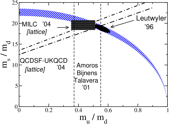
Figure 3: Light quark mass ratios. The light shaded band is the first quadrant of Leutwyler’s ellipse for $Q=22.7\pm 0.8$. Depicted are results from Leutwyler [83] and from the Lund group [85] as well as from two recent lattice calculations [86, 87]. Figure courtesy of Jürg Gasser.

For orientation, we give here the results from [83]:

$$\frac{m_{u}}{m_{d}}=0.553\pm 0.043~{},~{}~{}\displaystyle\frac{m_{s}}{m_{d}}=18.9\pm 0.8~{},~{}~{}\displaystyle\frac{m_{s}}{\hat{m}}=24.4\pm 1.5~{}.$$ (48)

It is remarkable that the up and down quark masses are so different – naively one thus would expect very sizeable strong isospin violation. However, this difference is effectively masked because it is so small compared to any hadronic scale, may it be $\Lambda_{\rm QCD}$, $m_{\rho}$ or $\Lambda_{\chi}$. The role of $\bar{s}s$ fluctuations on the ratio $m_{s}/\hat{m}$ is discussed in [88].

Another interesting recent result concerns the chiral expansion of the pion mass, which to leading order is given by the Gell-Mann–Oakes–Renner relation [89]

$$M_{\pi}^{2}=B\,(m_{u}+m_{d})+{\cal O}(m_{u,d}^{2})$$ (49)

and the corrections quadratic in the quark masses are parameterized by one LEC (called $\bar{\ell}_{3}$) that can also be obtained from data on $K_{\ell 4}$ decays (see next chapter). It was shown in Ref. [90] that $|\bar{\ell}_{3}|\leq 16$, which implies that the Gell-Mann–Oakes–Renner relation represents a good approximation – more than 94 % of the pion mass originate from the first term in its quark mass expansion. This also shows that the quark condensate is indeed the leading order parameter.

7.2 Goldstone boson scattering

The purest reaction to test the chiral dynamics of QCD is elastic pion–pion scattering at threshold. Since the pion three–momentum vanishes at threshold, the dual expansion of CHPT is given by one single small parameter, $M_{\pi}^{2}/(4\pi F_{\pi})^{2}\simeq 0.014$. The chiral expansion for the S-wave scattering lengths takes the form

$$a_{0}^{0}=\frac{7M_{\pi}^{2}}{32\pi F_{\pi}^{2}}~{}\Bigl{[}1+\Delta_{4}+\Delta_{6}\Bigr{]}+{\mathcal{O}}(M_{\pi}^{8})~{},$$

$$a_{0}^{2}=-\frac{M_{\pi}^{2}}{16\pi F_{\pi}^{2}}~{}\Bigl{[}1+\tilde{\Delta}_{4}+\tilde{\Delta}_{6}\Bigr{]}+{\mathcal{O}}(M_{\pi}^{8})~{},$$ (50)

where $\Delta_{4}$ and $\Delta_{6}$ collect the one– and two–loop corrections, first given in [92] and [72], respectively. The numerical evaluation of these corrections gives as central values (using $F_{\pi}=92.4\,$MeV)

$$a_{0}^{0}=0.159[1+0.26+0.10]=0.216~{},~{}~{}a_{0}^{2}=0.0454[1-0.02+0.00]=0.0445~{}.$$ (51)

The corrections in the isospin zero channel are remarkably large - this effect is completely understood in terms of the very strong final-state interactions that effectively generate a very broad pole at $\sqrt{s}\simeq 440\,$MeV far off the real axis. A layman’s discussion of this effect is provided in [93]. Quite in contrast, for isospin two the corrections have the expected small size. As remarked earlier, the most precise determination of these fundamental quantities of QCD comes from a combination of CHPT with dispersion relations, cf. Eq. (46). Fig. 4 collects the presently available theoretical and experimental information on the S-wave scattering lengths. The universal curve was already established from dispersion theoretical studies of $\pi\pi$ scattering in the sixties - it was found that all solutions that give phase shifts compatible with the $\rho$–meson and Regge behavior at high energies lead to a narrow band for $a_{0}^{0}$ and $a_{0}^{2}$ [94]. Shown is the updated universal curve from [74]. The experimental information stems from the analysis of $K_{\ell 4}$ decays [95], the measurement of the lifetime of pionium (an electromagnetic bound state of a $\pi^{+}\pi^{-}$ pair) [96] and the analysis of the aforementioned cusp in $K\to 3\pi$ decays [97]. Note that the preliminary analysis of $K_{e4}$ data from NA48/2 seems to be in conflict with these values.

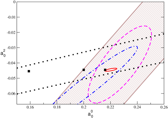
Figure 4: S-wave $\pi\pi$ scattering lengths: theory versus experiment. The filled squares give the central value of the tree [91], one-loop [92] and two-loop [72] calculations, respectively. The small solid ellipse is the result of Ref. [70]. The dotted lines denote the universal curve [74]. The hatched band is the results obtained from the DIRAC experiment (pionium lifetime) [96], the dot-dashed ellipse is the $K_{\ell 4}$ result from E865 [95] and the dashed ellipse the one obtained by the NA48/2 collaboration from analyzing the cusp in $K\to 3\pi$ [97]. Figure courtesy of Heiri Leutwyler.

The next simple and pure Goldstone boson process including also strange quarks is elastic pion–kaon scattering in the threshold region. Here, the situation is less satisfactory. First, the expansion parameter is now $M_{K}^{2}/(4\pi F_{\pi})^{2}\simeq 0.18$, which is sizably larger than in the $SU(2)$ case. The one– and two–loop corrections have been worked out in [98, 99] and [100], respectively. Furthermore, the Roy-Steiner equations for pion-kaon scattering with constraints from CHPT have been developed and analyzed in Refs. [101, 102]. It was found that most of the low–energy data are only in poor agreement with the solutions of the Roy–Steiner equations. Nevertheless, for the S-wave scattering lengths in the basis of physical isospin 1/2 and 3/2, the chiral expansion seems to converge reasonably well. A typical two–loop result from Ref. [100] is (note, however, that the paper also contains other fits with very different values)

$$a_{0}^{1/2}=0.220~{}[0.224\pm 0.022]~{},~{}~{}~{}10\,a_{0}^{3/2}=-0.47~{}[-0.448\pm 0.077]~{},$$ (52)

where the numbers in the brackets are the dispersive results of Ref. [102]. However, there persists a real puzzle. One can formulate an $SU(2)$ low-energy theorem for the isovector scattering length $a_{0}^{-}=(a_{0}^{1/2}-a_{0}^{3/2})/3$ [103],

$$a_{0}^{-}=\displaystyle\frac{M_{\pi}^{2}}{8\pi F_{\pi}^{2}(1+M_{\pi}/M_{K})}\left(1+{\cal O}(M_{\pi}^{2})\right)$$ (53)

which is not affected by kaon loop effects at next-to-leading order. (Note that there is a small caveat in this statement since the pertinent LECs have not been properly adapted from $SU(3)$ to $SU(2)$.) Since the final-state interactions in $K\pi$ scattering are weaker than in $\pi\pi$, one expects smaller corrections to $a_{0}^{-}$ than to $a_{0}^{0}$. This is also borne out by the one–loop calculation, the corrections is about 12 % [103, 104]. However, matching the $SU(3)$ two–loop representation of [100] to $SU(2)$, it was found that the subleading corrections to the low–energy theorem Eq. (53) are of the same size as the leading ones [105]. This might be related to the fact that a poor convergence was also found for some of the subthreshold parameters that parameterize the $\pi K$ scattering amplitude inside the Mandelstam triangle, see [100]. More work is needed to clarify the situation.

7.3 Neutral pion photoproduction

The chiral structure of QCD can also be analyzed in the presence of matter fields, in particular nucleons. Neutral pion photoproduction off nucleons in the threshold region, $\gamma N\to\pi^{0}N$ $(N=p,n)$, exhibits one of the most intriguing realizations of pion loop effects. In the threshold region, this process can be parameterized in terms of one complex S–wave and three complex P–wave multipoles, called $E_{0+}$ and $P_{1,2,3}$, respectively (for precise definitions, see e.g. [106] and references therein). To disentangle these multipoles, one has to measure differential cross sections and one polarization observable, like e.g. the photon asymmetry in $\vec{\gamma}p\to\pi^{0}p$. Historically, a low-energy theorem (LET) for the electric dipole amplitude was derived in the heydays of current algebra under certain analyticity (smoothness) assumptions [108, 109]. Measurements at Mainz, Saclay and Saskatoon seemed to be in conflict with this LET. It was, however, shown in Ref. [110] that the presence of the pions in loop graphs (more precisely in the so-called triangle diagram) generates infrared singularities in the Taylor coefficients of the invariant amplitude for $E_{0+}$ – invalidating the smoothness assumption made in Refs. [108, 109]. The correct form of the LET thus reads

$$\left\{E_{0+}^{\pi^{0}p}\atop E_{0+}^{\pi^{0}n}\right\} = -\displaystyle\frac{e\,g_{\pi N}}{8\pi m}\left[\mu\,F_{1}+\mu^{2}\,F_{2}+{\cal O}(\mu^{3})\right]~{},$$

$$F_{1}=\left(1\atop 0\right)~{},~{}~{}F_{2} = \!\!\!-\displaystyle\frac{1}{2}\left(3+\kappa^{p}\atop-\kappa^{n}\right)-\Delta\,\left(1\atop 1\right)~{},~{}~{}\Delta=\displaystyle\frac{m^{2}}{16F_{\pi}^{2}}\simeq 6.4~{},$$ (54)

in terms of the small parameter $\mu=M_{\pi}/m\simeq 1/7$ and $m$ is the nucleon mass. Furthermore, $g_{\pi N}\simeq 13$ is the strong pion–nucleon coupling constant and $\kappa_{p,n}$ the anomalous magnetic moment of the proton and neutron, respectively. The contribution $\sim\Delta$ is the novel pion loop effect first found in [110]. In fact, the terms $\sim\mu^{3}$ have also been worked out, besides loop contributions one has two polynomial terms which in the threshold region can be combined in one structure accompanied by one LEC. Consider now for definiteness neutral pion production off the proton. Fixing this LEC at the opening of the $\pi^{+}n$ threshold just $\approx 7\,$MeV above the $\pi^{0}p$ threshold, one obtains an excellent description of the threshold data for Re $E_{0+}$ as shown in Fig. 5. Also clearly visible is the cusp at the $\pi^{+}n$ threshold — its strength is directly proportional to the isovector (charge exchange) scattering length. Thus a more precise measurement of this cusp would give additional experimental information on zero energy pion–nucleon scattering (see also Ref. [111] for further discussion).

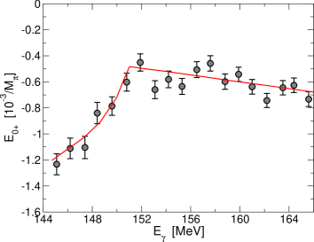
Figure 5: The real part of the electric dipole amplitude $E_{0+}$ in the threshold region. The solid line is the one–loop CHPT prediction [106, 113] and the data are the most recent measurement from MAMI [107].

Also, CHPT predicts the counterintuitive result that at threshold $|E_{0+}^{\pi^{0}n}|>|E_{0+}^{\pi^{0}p}|$. This prediction is vindicated by the measurement of coherent neutral pion production off the deuteron and utilizing CHPT for few–nucleon systems, see [112]. Note, however, that the chiral expansion for the electric dipole amplitude is not converging very well – this is another manifestation of strong final-state interactions, this time in the $\pi N$ system. Quite unexpectedly, in Ref. [106] novel LETs for the P–wave multipoles $P_{1,2}$ were found (including terms of order $\mu$) and the corrections of ${\cal O}(\mu^{2})$ were analyzed in [113]. These LETs are in good agreement with the data from Mainz (which performed so far the only polarization measurement that allows to disentangle $P_{1}$ from $P_{2}$), see e.g. [107] or [113] for detailed discussions. The comparison of the CHPT predictions with the most recent data from Mainz reads:

$$E_{0+} = -1.19\,~{}~{}[-1.23\pm 0.08\pm 0.03]~{},$$

$$\bar{P}_{1} = \phantom{-}9.67\,~{}~{}[9.46\pm 0.05\pm 0.28]~{},$$

$$\bar{P}_{2} = -9.6\,~{}~{}~{}[-9.5\pm 0.09\pm 0.28]~{},$$ (55)

in the conventional units of $10^{-3}/M_{\pi^{+}}$ and $10^{-3}/M_{\pi^{+}}^{2}$, respectively. Note also that the third P–wave multipole $P_{3}$ is given in terms of one third order LEC. $P_{3}$ is completely dominated by the excitation of the $\Delta$ resonance - in fact free fits to the data and estimating the strength of the LEC from resonance saturation give almost identical results. Recently, the relation between dispersion relations and the chiral representation for neutral pion photoproduction has been analyzed in the context of the so-called Fubini-Furlan-Rosetti sum rule, see Refs. [114, 115, 116]. In particular, relations between the LECs and the subtractions constants of the dispersion relations were derived and used to pin down some of the LECs with an unprecedented accuracy - cf. the discussion in Sec. 6. For similar studies combining dispersion relations and CHPT for elastic pion-nucleon scattering, see e.g. Refs. [117, 118]. In particular, in Ref. [118] the Roy-type equations for $\pi N$ scattering are written down — it just remains to solve them.

7.4 Connection to lattice QCD

QCD matrix elements can be calculated from first principles in the framework of lattice QCD. Space-time is approximated by a box of the size $V=L_{s}\times L_{s}\times L_{s}\times L_{t}$, where $L_{s}\,(L_{t})$ refers to the length in the spatial (temporal) directions. Furthermore, an UV cutoff is given by the inverse lattice spacing $a$. At present, typical lattice sizes and spacings are $L_{s}\simeq L_{t}\simeq 2\ldots 3\,$fm and $a\simeq 0.07\ldots 0.15\,$fm, respectively. In addition, it is very difficult to perform numerical simulations with light fermions, so the state-of-the-art calculations using various (improved) actions and modern algorithms have barely reached pion masses of about 250 MeV. In addition, exact chiral symmetry can only be implemented in the computer-time intensive domain wall [119] or overlap [120] formulations. Most results obtained so far are based on simulations using considerably heavier pions (and no exact chiral symmetry). To connect lattice results to the real world of continuum QCD, one has to perform the continuum limit ($a\to 0$), the thermodynamic limit $(V\to\infty)$ and chiral extrapolations from the unphysical to the physical quark masses. All this can be performed in the framework of suitably tailored effective field theories, which are variations of continuum chiral perturbation theory discussed so far, like e.g. staggered CHPT, Wilson CHPT and so on, via the intermediate step of the Symanzik effective action [121, 122]. Space does not allow to review all these interesting developments, we refer the reader to the recent comprehensive review by Sharpe [123] (for an early review on the CHPT treatment of finite volume effects, see [14]). Obviously, the lattice practioneers need CHPT – for truly ab initio calculations the quark mass dependence of the lattice results must be analyzed in terms of a model-independent approach like CHPT, in a regime of quark masses where it is applicable. Using resummation schemes or models to try to extend the range of applicability of CHPT inevitably induces an uncontrolled systematic uncertainty that should be avoided. It is indeed astonishing how often one finds in the literature statements of precise determinations of hadron properties based on extrapolation functions that are not rooted in QCD or are at best models with a questionable relation to QCD. In what follows, we will address the issue to what extent chiral perturbation theory representations and lattice QCD results are already overlapping.

Chiral perturbation theory provides unambiguous chiral extrapolation functions, parameterized in terms of the pertinent LECs. Ideally, one would like to perform global fits to a large variety of observables since these are interrelated through the appearance of certain LECs. At present, however, this is not yet possible and for a variety of applications it is mandatory to include phenomenological input for some of the LECs – an example will be given below. It should be noted that frequently in the literature one–loop extrapolation functions are used for pion masses well outside the regime of their applicability. As a matter of fact, most pion and kaon Green functions have been worked out at two–loop accuracy in the continuum (for a review, see [24]) and considerable progress has been reported for many of these quantities for partially quenched QCD, in which one allows for different values of the valence and the sea quarks, see e.g. [124, 125, 126, 127]. Clearly, with increasing quark masses the CHPT representations become increasingly inaccurate – and this is in fact a strength of the effective field theory, in that it provides a measure of the theoretical uncertainty. Let us illustrate these issues for the pion decay constant $F_{\pi}$. Its special role for the spontaneous symmetry breaking was already explained in Sec. 2. Its analytic form at two-loop order in the continuum is [62, 128]

$$F_{\pi} = F\,\left[1+X\,\tilde{\Delta}^{(4)}+X^{2}\,\tilde{\Delta}^{(6)}\right]$$

$$= F\,\biggl{\{}1+X\,\left[\tilde{L}+\tilde{\ell}_{4}\right]+X^{2}\,\left[-\frac{3}{4}\tilde{L}^{2}+\tilde{L}\left(-\frac{7}{6}\tilde{\ell}_{1}-\frac{4}{3}\tilde{\ell}_{2}+\tilde{\ell}_{4}-\frac{29}{12}\right)\right.$$

$$\qquad\qquad\qquad\qquad\qquad\qquad\left.+\frac{1}{2}\tilde{\ell}_{3}\tilde{\ell}_{4}+\frac{1}{12}\tilde{\ell}_{1}-\frac{1}{3}\tilde{\ell}_{2}-\frac{13}{192}+\tilde{r}(\mu)\right]\biggr{\}}~{},$$

$$X = \frac{M_{\pi}^{2}}{16\pi^{2}F^{2}}~{},~{}~{}\tilde{L}=\log\frac{\mu^{2}}{M_{\pi}^{2}}~{},~{}~{}\tilde{\ell}_{i}=\log\frac{\Lambda_{i}^{2}}{\mu^{2}}~{},$$ (56)

where $\tilde{r}(\mu)$ is a combination of dimension six LECs. Note that – in contrast to common lore – the number of new LECs does not explode when going to higher orders when one considers specific observables. With $\Lambda_{1}=0.12_{-0.03}^{+0.04}\,$GeV, $\Lambda_{2}=1.20_{-0.06}^{+0.06}\,$GeV, $\Lambda_{3}=0.59_{-0.41}^{+1.40}\,$GeV, $\Lambda_{4}=1.25_{-0.03}^{+0.04}\,$GeV, $\tilde{r}(\mu)=0\pm 3$ from resonance saturation, varying the scale of dimensional regularization $\mu$ between 500 MeV and 1 GeV and using $F_{\pi}=92.4\pm 0.3\,$MeV, one obtains the (yellow) band between the solid lines in Fig. 6.

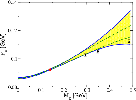
Figure 6: Pion (quark) mass dependence of the pion decay constant – lattice results from Ref. [129] (circles) in comparison to the two–loop CHPT result from Ref. [128] (hatched area). The one–loop band which is obtained by varying $\tilde{\ell}_{4}$ is given by the dashed lines. The diamond is the physical point.

For comparison, the dashed lines correspond to the one–loop result. Note that for pion masses below 300 MeV, the one– and two–loop representations are essentially equivalent, but for higher pion masses it is important to include the two–loop corrections for a realistic assessment of the theoretical uncertainty. This is consistent with expectations based on naive dimensional analysis, the expansion parameter is $X=0.01,0.07,0.18$ for $M_{\pi}=139.57,300,500\,$MeV, respectively. For orientation, we also show the recent lattice results from Ref. [129], in that paper, the one–loop representation for $M_{\pi}$ and $F_{\pi}$ is used and the LEC $\tilde{\ell}_{4}$ is extracted with an accuracy of a few percent. This appears optimistic if one accounts for the two–loop corrections at these pion masses as shown in Fig. 6. Other collaboration like QCDSF, ETM, CERN-Roma, $\ldots$ have also obtained results for $F_{\pi}$ at low pion masses, however, these “data” have not been finally analyzed by the time this review was written (see e.g. Ref. [130] for some of these preliminary results).

Matters are somewhat different in the baryon (nucleon) sector for two reasons. Although a multitude of ground-state (and some excited state) properties have been simulated, most CHPT calculations have been performed to one–loop accuracy. Further, in these extrapolation functions one has even and odd powers of the expansion parameter(s) and correspondingly more LECs. For these reasons chiral extrapolations can only be performed over a smaller range of pion masses with a tolerable uncertainty as compared to the meson sector. Space does not allow for an overall review here, we refer the reader to Ref. [40]. We briefly discuss the quark mass dependence of the nucleon axial-vector coupling $g_{A}$ here, since a variety of lattice data exists for pion masses ranging from 340 MeV to 1 GeV. Also, the two–loop representation of $g_{A}$ has recently been published [131]. This allows one to discuss some subtleties that can arise in the chiral expansion of certain observables. The pion mass expansion of $g_{A}$ takes the form

$$g_{A}=g_{0}\,\biggl{\{}\underbrace{1}_{\rm tree}+\underbrace{\Delta^{(2)}+\Delta^{(3)}}_{\rm 1-loop}+\underbrace{\Delta^{(4)}+\Delta^{(5)}}_{\rm 2-loop}\biggr{\}}+{\cal O}(M_{\pi}^{6})~{},$$ (57)

where $g_{0}$ is the chiral limit value of $g_{A}$ and $\Delta^{(n)}$ collects the corrections that are proportional to $M_{\pi}^{n}$. At one–loop order, the chiral representation of $g_{A}$ contains $g_{0}$, one combination of dimension two LECs ($c_{2}+c_{3}$) and one dimension three LEC ($d_{16}$). The latter two can be determined from the analysis of $\pi N\to\pi N$ and $\pi N\to\pi\pi N$, respectively. This is one of the cases where it is mandatory to include such phenomenological information to analyze the chiral expansion of a given observable. The one–loop representation is dominated by the $M_{\pi}^{3}$-term as the pion mass increases – one is therefore not able to connect to the lattice results, which show a very weak dependence of $g_{A}$ on the pion mass.

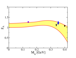
Figure 7: Pion mass dependence of the axial-vector coupling – lattice results from LHPC/MILC [132] (triangles) and QCDSF [133] (inverted triangles) in comparison to the two–loop CHPT result from Ref. [131] (filled area). The circle is the physical point.

At two loops, one has further operators accompanied by certain combinations of LECs. The dominant contributions to these stem from $1/m$ corrections to the lower order LECs. The remaining pieces can only be estimated assuming naturalness. Demanding further that the trend of the lattice data is followed, one arrives at the (yellow) band shown in Fig. 7. The width of the band is a consequence of this condition – there are strong cancellations between the various contributions. Also, one sees that the range of applicability of the chiral extrapolation function and the lattice results barely overlap, to arrive at precision results for $g_{A}$, pion masses of less than 300 MeV are mandatory. In view of this, the claim of Ref. [132] that $g_{A}$ has been calculated and precisely determined in the chiral regime appears overly optimistic - more data at lower pion masses are called for to substantiate such claims. We also note that these strong cancellations between various orders were first found in an EFT approach including the $\Delta(1232)$ as an active degree of freedom and counting the nucleon-delta mass splitting $m_{\Delta}-m_{N}\simeq 3F_{\pi}$ as an additional small parameter at leading one–loop order, see [134] and the recent update [135]. The claims in these papers that one can truthfully represent the chiral expansion of $g_{A}$ in leading one-loop order for pion masses up to 700 MeV once the delta is included are unfounded – the resummation of some subset of corrections induces an uncontrolled uncertainty because other higher order effects are ignored. A beautiful example for this is provided by the cancellations of delta contributions and higher order $\pi N$ loop effects in the nucleons’ magnetic polarizabilities [136]. Note also that finite volume corrections for $g_{A}$, which are essential for connecting the lattice results with the real world, are discussed e.g. in Refs. [137, 138, 139].

Finally, we note that CHPT practioneers also need the lattice. In particular for non-leptonic weak meson interactions and in the baryon sector, the amount of precise phenomenological information is limited. Therefore, it appears impossible to pin down all LECs, in particular the symmetry breakers, cf. Sec. 4. After the pioneering work of Ref. [140] in the mid-nineties, the ALPHA collaboration has reported considerable progress in the lattice determination of the next-to-leading order LECs in the meson sector [141]. Further work on the leading order LECs for $\Delta S=1$ transitions are reported in Ref. [142] and a method to determine the pion–nucleon LEC $c_{3}$ was suggested in Ref. [143]. In our opinion, more effort should be invested in the determination of LECs from lattice studies, and this would further tighten the interplay between the CHPT and the lattice communities. This is important because it will take a long time before complicated processes or reactions with many external probes will be amenable to lattice simulations.

References

- [1] R. D. Peccei and H. R. Quinn, Phys. Rev. Lett. 38, 1440 (1977).
- [2] C. Vafa and E. Witten, Nucl. Phys. B 234, 173 (1984).
- [3] C. McNeile, Phys. Lett. B 619, 124 (2005) [arXiv:hep-lat/0504006].
- [4] T. Banks and A. Casher, Nucl. Phys. B 169, 103 (1980).
- [5] H. Leutwyler and A. Smilga, Phys. Rev. D 46 (1992) 5607.
- [6] J. Stern, arXiv:hep-ph/9801282.
- [7] J. Goldstone, Nuovo Cim. 19, 154 (1961).
- [8] J. Goldstone, A. Salam and S. Weinberg, Phys. Rev. 127, 965 (1962).
- [9] J. Stern, arXiv:hep-ph/0611127.
- [10] M. Gell-Mann and Y. Ne’eman, The Eightfold Way, W. A. Benjamin (New York, 1964).
- [11] K. Fujikawa, Phys. Rev. D 29, 285 (1984).
- [12] J. F. Donoghue, CERN-TH-5667-90 Presented at Int. School of Low-Energy Antiprotons, Erice, Italy, Jan 25-31, 1990
- [13] J. Bijnens, Int. J. Mod. Phys. A 8 (1993) 3045.
- [14] U.-G. Meißner, Rept. Prog. Phys. 56, 903 (1993) [arXiv:hep-ph/9302247].
- [15] H. Leutwyler, arXiv:hep-ph/9406283.
- [16] G. Ecker, Prog. Part. Nucl. Phys. 35, 1 (1995) [arXiv:hep-ph/9501357].
- [17] V. Bernard, N. Kaiser and U.-G. Meißner, Int. J. Mod. Phys. E 4, 193 (1995) [arXiv:hep-ph/9501384].
- [18] A. Pich, Rept. Prog. Phys. 58, 563 (1995) [arXiv:hep-ph/9502366].
- [19] J. Gasser, Nucl. Phys. Proc. Suppl. 86, 257 (2000) [arXiv:hep-ph/9912548].
- [20] H. Leutwyler, arXiv:hep-ph/0008124.
- [21] S. Scherer, Adv. Nucl. Phys. 27, 277 (2003) [arXiv:hep-ph/0210398].
- [22] J. Gasser, Lect. Notes Phys. 629, 1 (2004) [arXiv:hep-ph/0312367].
- [23] G. Ecker, AIP Conf. Proc. 806, 1 (2006) [arXiv:hep-ph/0510134].
- [24] J. Bijnens, arXiv:hep-ph/0604043.
- [25] S. Weinberg, PhysicaA 96, 327 (1979).
- [26] J. Gasser and H. Leutwyler, Annals Phys. 158, 142 (1984).
- [27] J. Gasser and H. Leutwyler, Nucl. Phys. B 250, 465 (1985).
- [28] H. Leutwyler, Annals Phys. 235, 165 (1994) [arXiv:hep-ph/9311274].
- [29] S. Weinberg, arXiv:hep-ph/9412326.
- [30] N. H. Fuchs, H. Sazdjian and J. Stern, Phys. Lett. B 269, 183 (1991).
- [31] J. Bijnens, G. Colangelo and G. Ecker, JHEP 9902, 020 (1999) [arXiv:hep-ph/9902437].
- [32] J. Gasser and H. Leutwyler, Phys. Rept. 87, 77 (1982).
- [33] R. Urech, Nucl. Phys. B 433, 234 (1995) [arXiv:hep-ph/9405341].
- [34] U.-G. Meißner, G. Müller and S. Steininger, Phys. Lett. B 406 (1997) 154 [Erratum-ibid. B 407 (1997) 454] [arXiv:hep-ph/9704377].
- [35] M. Knecht, H. Neufeld, H. Rupertsberger and P. Talavera, Eur. Phys. J. C 12, 469 (2000) [arXiv:hep-ph/9909284].
- [36] J. Schweizer, JHEP 0302, 007 (2003) [arXiv:hep-ph/0212188].
- [37] J. Gasser, A. Rusetsky and I. Scimemi, Eur. Phys. J. C 32, 97 (2003) [arXiv:hep-ph/0305260].
- [38] U.-G. Meißner, in Shifman, M. (ed.): At the frontier of particle physics, vol. 1, pp. 417-505. [arXiv:hep-ph/0007092].
- [39] S. Scherer, Int. J. Mod. Phys. A 21, 881 (2006) [arXiv:hep-ph/0509186].
- [40] V. Bernard, “Chiral perturbation theory and baryon properties,” commissioned article for Prog. Nucl. Part. Phys. .
- [41] G. Müller and U.-G. Meißner, Nucl. Phys. B 556, 265 (1999) [arXiv:hep-ph/9903375].
- [42] J. Gasser, M. A. Ivanov, E. Lipartia, M. Mojzis and A. Rusetsky, Eur. Phys. J. C 26, 13 (2002) [arXiv:hep-ph/0206068].
- [43] H. Georgi, Ann. Rev. Nucl. Part. Sci. 43, 209 (1993).
- [44] D. Espriu and J. Matias, Nucl. Phys. B 418, 494 (1994) [arXiv:hep-th/9307086].
- [45] J. Gasser and A. Zepeda, Nucl. Phys. B 174, 445 (1980).
- [46] J. Bijnens, G. Colangelo and G. Ecker, Annals Phys. 280, 100 (2000) [arXiv:hep-ph/9907333].
- [47] G. Ecker, J. Gasser, A. Pich and E. de Rafael, Nucl. Phys. B 321, 311 (1989).
- [48] G. Ecker, J. Gasser, H. Leutwyler, A. Pich and E. de Rafael, Phys. Lett. B 223, 425 (1989).
- [49] J. F. Donoghue, C. Ramirez and G. Valencia, Phys. Rev. D 39, 1947 (1989).
- [50] K. Kampf and B. Moussallam, arXiv:hep-ph/0604125.
- [51] V. Cirigliano, G. Ecker, M. Eidemuller, R. Kaiser, A. Pich and J. Portoles, arXiv:hep-ph/0603205.
- [52] V. Bernard, N. Kaiser and U.-G. Meißner, Nucl. Phys. A 615, 483 (1997) [arXiv:hep-ph/9611253].
- [53] E. Epelbaum, U.-G. Meißner, W. Glöckle and C. Elster, Phys. Rev. C 65, 044001 (2002) [arXiv:nucl-th/0106007].
- [54] V. Bernard, T. R. Hemmert and U.-G. Meißner, Nucl. Phys. A 732, 149 (2004) [arXiv:hep-ph/0307115].
- [55] J. Gasser and U.-G. Meißner, Nucl. Phys. B 357, 90 (1991).
- [56] J. F. Donoghue, J. Gasser and H. Leutwyler, Nucl. Phys. B 343, 341 (1990).
- [57] M. A. B. Beg and A. Zepeda, Phys. Rev. D 6, 2912 (1972).
- [58] T. N. Truong, “Modern Application Of Dispersion Relation: Chiral Perturbation Versus Dispersion Technique,” CERN-TH-4748/87
- [59] J. F. Donoghue and B. R. Holstein, Phys. Rev. D 48 (1993) 137 [arXiv:hep-ph/9302203].
- [60] J. F. Donoghue, arXiv:hep-ph/9506205.
- [61] J. Bijnens and P. Talavera, JHEP 0203, 046 (2002) [arXiv:hep-ph/0203049].
- [62] J. Bijnens, G. Colangelo and P. Talavera, JHEP 9805, 014 (1998) [arXiv:hep-ph/9805389].
- [63] B. Moussallam, Eur. Phys. J. C 14, 111 (2000) [arXiv:hep-ph/9909292].
- [64] U.-G. Meißner and J. A. Oller, Nucl. Phys. A 679, 671 (2001) [arXiv:hep-ph/0005253].
- [65] M. Frink, B. Kubis and U.-G. Meißner, Eur. Phys. J. C 25, 259 (2002) [arXiv:hep-ph/0203193].
- [66] B. Ananthanarayan, I. Caprini, G. Colangelo, J. Gasser and H. Leutwyler, Phys. Lett. B 602, 218 (2004) [arXiv:hep-ph/0409222].
- [67] T. A. Lähde and U.-G. Meißner, Phys. Rev. D 74, 034021 (2006) [arXiv:hep-ph/0606133].
- [68] H. Lehmann, Phys. Lett. B 41, 529 (1972).
- [69] S. M. Roy, Phys. Lett. B 36, 353 (1971).
- [70] G. Colangelo, J. Gasser and H. Leutwyler, Phys. Lett. B 488, 261 (2000) [arXiv:hep-ph/0007112].
- [71] M. Knecht, B. Moussallam, J. Stern and N. H. Fuchs, Nucl. Phys. B 457, 513 (1995) [arXiv:hep-ph/9507319].
- [72] J. Bijnens, G. Colangelo, G. Ecker, J. Gasser and M. E. Sainio, Phys. Lett. B 374, 210 (1996) [arXiv:hep-ph/9511397].
- [73] J. Bijnens, G. Colangelo, G. Ecker, J. Gasser and M. E. Sainio, Nucl. Phys. B 508 (1997) 263 [Erratum-ibid. B 517 (1998) 639] [arXiv:hep-ph/9707291].
- [74] B. Ananthanarayan, G. Colangelo, J. Gasser and H. Leutwyler, Phys. Rept. 353 (2001) 207 [arXiv:hep-ph/0005297].
- [75] S. Descotes-Genon, N. H. Fuchs, L. Girlanda and J. Stern, Eur. Phys. J. C 24 (2002) 469 [arXiv:hep-ph/0112088].
- [76] R. Kaminski, J. R. Pelaez and F. J. Yndurain, Phys. Rev. D 74 (2006) 014001 [arXiv:hep-ph/0603170].
- [77] J. R. Pelaez and F. J. Yndurain, Phys. Rev. D 68 (2003) 074005 [arXiv:hep-ph/0304067].
- [78] U.-G. Meißner, Nucl. Phys. A 629, 72C (1998) [arXiv:hep-ph/9706367].
- [79] N. Cabibbo, Phys. Rev. Lett. 93 (2004) 121801 [arXiv:hep-ph/0405001].
- [80] N. Cabibbo and G. Isidori, JHEP 0503 (2005) 021 [arXiv:hep-ph/0502130].
- [81] G. Colangelo, J. Gasser, B. Kubis and A. Rusetsky, Phys. Lett. B 638 (2006) 187 [arXiv:hep-ph/0604084].
- [82] J. F. Donoghue, Ann. Rev. Nucl. Part. Sci. 39, 1 (1989).
- [83] H. Leutwyler, Phys. Lett. B 378 (1996) 313 [arXiv:hep-ph/9602366].
- [84] D. B. Kaplan and A. V. Manohar, Phys. Rev. Lett. 56, 2004 (1986).
- [85] G. Amoros, J. Bijnens and P. Talavera, Nucl. Phys. B 602 (2001) 87 [arXiv:hep-ph/0101127].
- [86] C. Aubin et al. [MILC Collaboration], Phys. Rev. D 70, 114501 (2004) [arXiv:hep-lat/0407028].
- [87] M. Göckeler, R. Horsley, A. C. Irving, D. Pleiter, P. E. L. Rakow, G. Schierholz and H. Stuben [QCDSF Collaboration], Phys. Lett. B 639, 307 (2006) [arXiv:hep-ph/0409312].
- [88] S. Descotes-Genon, N. H. Fuchs, L. Girlanda and J. Stern, Eur. Phys. J. C 34, 201 (2004) [arXiv:hep-ph/0311120].
- [89] M. Gell-Mann, R. J. Oakes and B. Renner, Phys. Rev. 175, 2195 (1968).
- [90] G. Colangelo, J. Gasser and H. Leutwyler, Phys. Rev. Lett. 86 (2001) 5008 [arXiv:hep-ph/0103063].
- [91] S. Weinberg, Phys. Rev. Lett. 17, 616 (1966).
- [92] J. Gasser and H. Leutwyler, Phys. Lett. B 125, 325 (1983).
- [93] U.-G. Meißner, Comments Nucl. Part. Phys. 20, 119 (1991).
- [94] D. Morgan and G. Shaw, Nucl. Phys. B 10, 261 (1969).
- [95] S. Pislak et al., Phys. Rev. D 67 (2003) 072004 [arXiv:hep-ex/0301040].
- [96] B. Adeva et al. [DIRAC Collaboration], Phys. Lett. B 619 (2005) 50 [arXiv:hep-ex/0504044].
- [97] J. R. Batley et al. [NA48/2 Collaboration], Phys. Lett. B 633 (2006) 173 [arXiv:hep-ex/0511056].
- [98] V. Bernard, N. Kaiser and U.-G. Meißner, Phys. Rev. D 43, 2757 (1991).
- [99] V. Bernard, N. Kaiser and U.-G. Meißner, Nucl. Phys. B 357, 129 (1991).
- [100] J. Bijnens, P. Dhonte and P. Talavera, JHEP 0405, 036 (2004) [arXiv:hep-ph/0404150].
- [101] B. Ananthanarayan, P. Buettiker and B. Moussallam, Eur. Phys. J. C 22 (2001) 133 [arXiv:hep-ph/0106230].
- [102] P. Buettiker, S. Descotes-Genon and B. Moussallam, Eur. Phys. J. C 33, 409 (2004) [arXiv:hep-ph/0310283].
- [103] A. Roessl, Nucl. Phys. B 555 (1999) 507 [arXiv:hep-ph/9904230].
- [104] B. Kubis and U.-G. Meißner, Phys. Lett. B 529, 69 (2002) [arXiv:hep-ph/0112154].
- [105] J. Schweizer, Phys. Lett. B 625, 217 (2005) [arXiv:hep-ph/0507323].
- [106] V. Bernard, N. Kaiser and U.-G. Meißner, Z. Phys. C 70 (1996) 483 [arXiv:hep-ph/9411287].
- [107] A. Schmidt et al., Phys. Rev. Lett. 87, 232501 (2001) [arXiv:nucl-ex/0105010].
- [108] P. De Baenst, Nucl. Phys. B 24, 633 (1970).
- [109] A. I. Vainshtein and V. I. Zakharov, Nucl. Phys. B 36, 589 (1972).
- [110] V. Bernard, N. Kaiser, J. Gasser and U.-G. Meißner, Phys. Lett. B 268, 291 (1991).
- [111] A. M. Bernstein, E. Shuster, R. Beck, M. Fuchs, B. Krusche, H. Merkel and H. Ströher, Phys. Rev. C 55, 1509 (1997) [arXiv:nucl-ex/9610005].
- [112] S. R. Beane, V. Bernard, T. S. H. Lee, U.-G. Meißner and U. van Kolck, Nucl. Phys. A 618 (1997) 381 [arXiv:hep-ph/9702226].
- [113] V. Bernard, N. Kaiser and U.-G. Meißner, Eur. Phys. J. A 11 (2001) 209 [arXiv:hep-ph/0102066].
- [114] B. Pasquini, D. Drechsel and L. Tiator, Eur. Phys. J. A 23, 279 (2005) [arXiv:nucl-th/0412038].
- [115] V. Bernard, B. Kubis and U.-G. Meißner, Eur. Phys. J. A 25, 419 (2005) [arXiv:nucl-th/0506023].
- [116] B. Pasquini, D. Drechsel and L. Tiator, Eur. Phys. J. A 27, 231 (2006) [arXiv:nucl-th/0603006].
- [117] P. Büttiker and U.-G. Meißner, Nucl. Phys. A 668, 97 (2000) [arXiv:hep-ph/9908247].
- [118] T. Becher and H. Leutwyler, JHEP 0106, 017 (2001) [arXiv:hep-ph/0103263].
- [119] D. B. Kaplan, Phys. Lett. B 288, 342 (1992) [arXiv:hep-lat/9206013].
- [120] R. Narayanan and H. Neuberger, Nucl. Phys. B 443, 305 (1995) [arXiv:hep-th/9411108].
- [121] K. Symanzik, Nucl. Phys. B 226, 187 (1983).
- [122] K. Symanzik, Nucl. Phys. B 226, 205 (1983).
- [123] S. R. Sharpe, arXiv:hep-lat/0607016.
- [124] J. Bijnens, N. Danielsson and T. A. Lähde, Phys. Rev. D 70, 111503 (2004) [arXiv:hep-lat/0406017].
- [125] J. Bijnens and T. A. Lähde, Phys. Rev. D 71, 094502 (2005) [arXiv:hep-lat/0501014].
- [126] J. Bijnens and T. A. Lähde, Phys. Rev. D 72, 074502 (2005) [arXiv:hep-lat/0506004].
- [127] J. Bijnens, N. Danielsson and T. A. Lähde, Phys. Rev. D 73, 074509 (2006) [arXiv:hep-lat/0602003].
- [128] G. Colangelo and S. Dürr, Eur. Phys. J. C 33, 543 (2004) [arXiv:hep-lat/0311023].
- [129] S. R. Beane, P. F. Bedaque, K. Orginos and M. J. Savage [NPLQCD Collaboration], Phys. Rev. D 73, 054503 (2006) [arXiv:hep-lat/0506013].
- [130] U.-G. Meißner and G. Schierholz, arXiv:hep-lat/0611072.
- [131] V. Bernard and U.-G. Meißner, Phys. Lett. B 639, 278 (2006) [arXiv:hep-lat/0605010].
- [132] R. G. Edwards et al. [LHPC Collaboration], Phys. Rev. Lett. 96, 052001 (2006) [arXiv:hep-lat/0510062].
- [133] M. Göckeler, private communication.
- [134] T. R. Hemmert, M. Procura and W. Weise, Phys. Rev. D 68, 075009 (2003) [arXiv:hep-lat/0303002].
- [135] M. Procura, B. U. Musch, T. R. Hemmert and W. Weise, arXiv:hep-lat/0610105.
- [136] V. Bernard, N. Kaiser, A. Schmidt and U.-G. Meißner, Phys. Lett. B 319, 269 (1993) [arXiv:hep-ph/9309211].
- [137] S. R. Beane and M. J. Savage, Phys. Rev. D 70, 074029 (2004) [arXiv:hep-ph/0404131].
- [138] G. Colangelo, A. Fuhrer and C. Haefeli, Nucl. Phys. Proc. Suppl. 153, 41 (2006) [arXiv:hep-lat/0512002].
- [139] A. A. Khan et al., arXiv:hep-lat/0603028.
- [140] S. Myint and C. Rebbi, Nucl. Phys. B 421, 241 (1994) [arXiv:hep-lat/9401009].
- [141] J. Heitger, R. Sommer and H. Wittig [ALPHA Collaboration], Nucl. Phys. B 588, 377 (2000) [arXiv:hep-lat/0006026].
- [142] L. Giusti, P. Hernandez, M. Laine, P. Weisz and H. Wittig, JHEP 0404 (2004) 013 [arXiv:hep-lat/0402002].
- [143] P. F. Bedaque, H. W. Grießhammer and G. Rupak, Phys. Rev. D 71, 054015 (2005) [arXiv:hep-lat/0407009].