DIRECT WIMP DETECTION IN DIRECTIONAL EXPERIMENTS

Abstract

The recent WMAP data have confirmed that exotic dark matter together with the vacuum energy (cosmological constant) dominate in the flat Universe. Thus the direct dark matter search, consisting of detecting the recoiling nucleus, is central to particle physics and cosmology. Modern particle theories naturally provide viable cold dark matter candidates with masses in the GeV-TeV region. Supersymmetry provides the lightest supersymmetric particle (LSP), theories in extra dimensions the lightest Kaluza-Klein particle (LKP) etc. In such theories the expected rates are much lower than the present experimental goals. So one should exploit characteristic signatures of the reaction, such as the modulation effect and, in directional experiments, the correlation of the event rates with the sun’s motion. In standard non directional experiments the modulation is small, less than two per cent and the location of the maximum depends on the unknown particle’s mass. In directional experiments, in addition to the forward-backward asymmetry due to the sun’s motion, one expects a larger modulation, which depends on the direction of observation. We study such effects both in the case of a light and a heavy target. Furthermore, since it now appears that the planned experiments will be partly directional, in the sense that they can only detect the line of the recoiling nucleus, but not the sense of direction on it, we study which of the above mentioned interesting features, if any, will persist in these less ambitious experiments.

I Introduction

The combined MAXIMA-1 MAX , BOOMERANG BOO , DASI DAS and COBE/DMR Cosmic Microwave Background (CMB) observations Smoot et al (1992) (COBE Collaboration) imply that the Universe is flat Jaffe et al (2001) and that most of the matter in the Universe is Dark Spergel et al (2003). i.e. exotic. These results have been confirmed and improved by the recent WMAP data WMA . Combining the the data of these quite precise experiments, crudely speaking, one finds:

$$\Omega_{b}=0.05,\Omega_{CDM}=0.25,\Omega_{\Lambda}=0.70$$

Since the non exotic component cannot exceed $40\%$ of the CDM  Bennett et al. (1995), there is room for the exotic WIMP’s (Weakly Interacting Massive Particles).

Even though there exists firm indirect evidence for a halo of dark matter in galaxies from the observed rotational curves, it is essential to directly detect Goodman and Witten (1985)-Kosmas and Vergados (1997) such matter. Until dark matter is actually detected, we shall not be able to exclude the possibility that the rotation curves result from a modification of the laws of nature as we currently view them. This makes it imperative that we invest a maximum effort in attempting to detect dark matter whenever it is possible. Furthermore such a direct detection will also unravel the nature of the constituents of dark matter. The possibility of such detection, however, depends on the nature of the dark matter constituents.

Supersymmetry naturally provides candidates for the dark matter constituents Goodman and Witten (1985)-Ellis and Roszkowski (1992). In the most favored scenario of supersymmetry the LSP (Lightest Supersymmetric Particle) can be simply described as a Majorana fermion, a linear combination of the neutral components of the gauginos and higgsinos Goodman and Witten (1985)-ref . In most calculations the neutralino is assumed to be primarily a gaugino, usually a bino.

Since the WIMP’s are expected to be very massive, $m_{WIMP}\geq 30GeV$, and extremely non relativistic, with average kinetic energy $\prec T\succ\approx 50KeV(m_{WIMP}/100GeV)$, they are not likely to excite the nucleus. So they can be directly detected mainly via the recoiling of a nucleus (A,Z) in elastic scattering. The event rate for such a process can be computed from the following ingredients:

1. An effective Lagrangian at the elementary particle (quark) level obtained in the framework of the prevailing particle theory. For supersymmetry this is achieved as described , e.g., in Refs ref ; Vergados (1996).

2. A well defined procedure for transforming the amplitude obtained using the previous effective Lagrangian from the quark to the nucleon level, i.e. a quark model for the nucleon. This step in SUSY models is not trivial, since the obtained results depend crucially on the content of the nucleon in quarks other than u and d.

3. Knowledge of the relevant nuclear matrix elements Res $-$Divari et al. (2000), obtained with as reliable as possible many body nuclear wave functions. Fortunately in the case of the scalar coupling, which is viewed as the most important, the situation is a bit simpler, since then one needs only the nuclear form factor.

4. Knowledge of the WIMP density in our vicinity and its velocity distribution. Since the essential input here comes from the rotational curves, dark matter candidates other than the LSP (neutralino) are also characterized by similar parameters.

In the standard nuclear recoil experiments one has the problem that the reaction of interest does not have a characteristic feature to distinguish it from the background. So for the expected low counting rates the background is a formidable problem. Some special features of the LSP-nuclear interaction can be exploited to reduce the background problems. Such are:

• The modulation effect.
  This yields e periodic signal due to the motion of the earth around the sun. Unfortunately this effect is small, $<2\%$ for most targets. Furthermore it is inevitable to have backgrounds with a seasonal variation.

• Transitions to excited states.
  In this case one need not measure nuclear recoils, but the de-excitation $\gamma$ rays. This can happen only in vary special cases since the average WIMP energy is too low to excite the nucleus. It has, however, been found that in the special case of the target ¹²⁷I such a process is feasible Vergados et al. (2005) with branching ratios around $5\%$.

• Detection of electrons produced during the WIMP-nucleus collision.
  It turns out, however, that this production peaks at very low energies. So only gaseous TPC detectors can reach the desired level of $100$eV. In such a case the number of electrons detected may exceed the number of recoils for a target with high $Z$ Vergados and Ejiri (2005),Moustakidis et al. (2005).

• Detection of hard X-rays produced when the inner shell holes are filled.
  It has been found EMV that in the previous mechanism inner shell electrons can be ejected. These holes can be filled by the Auger process or X-ray emission. For a target like Xe these X-rays are in the $30$keV region with the rate of about 0.1 per recoil for a WIMP mass of $100$ GeV.

In the present paper we will focus on the characteristic signatures of the WIMP nucleus interaction, which will manifest themselves in directional recoil experiments, i.e. experiments in which the direction of the recoiling nucleus is observed DRI ,Shimizu et al. (2003),KUD ,Morgan and Green (2005),Copi et al. (1999),Copi and Krauss (2001),Vergados (2003),Vergados (2004). We will concentrate on the standard Maxwell-Boltzmann (M-B) distribution for the WIMPs of our galaxy and we will not be concerned with other non thermal distributions, even though they may yield stronger directional signals. Among those one should mention the late infall of dark matter into the galaxy, i.e caustic rings Sikivie (1999, 1998); Vergados (2001); Green (2001); Gelmini and Gondolo (2001), dark matter orbiting the Sun Copi et al. (1999) and Sagittarius dark matter Green (2002).

We will present our results in such a fashion that they do not depend on the specific properties of the dark matter candidate, except that the candidate is cold and massive, $m_{WIMP}\succeq 10$ GeV. So the only parameters which count is the reduced mass, the nuclear form factor and the velocity distribution. So our results apply to all WIMPs. In a previous paper we have found that the observed rate is correlated with the direction of the sun’s motion Vergados (2003, 2004). On top of this one will observe a time dependent variation of the rate due to the motion of the earth. Those features cannot be masked by any known background. Unfortunately, however, even the most ambitious of the planned experiments are not expected soon to distinguish the two possible senses along the line of nuclear recoil SPO . Such experiments cannot, e.g., measure the backward-forward asymmetry. on this occasion we will extend our previous directional calculations Vergados (2003)-Vergados (2004) and explore, which characteristics, if any, of the previous calculation persist, if the rates for both senses of the nuclear recoil are summed up.

II Rates

Before computing the event rates for WIMP nucleus scattering we should discuss the kinematics. In the case of the WIMP-nucleus collision we find that the momentum transfer to the nucleus is given by

$$q=2\mu_{r}\upsilon\cos{\theta},$$ (1)

where $\theta$ is the angle between the WIMP velocity and the momentum of the outgoing nucleus and $\mu_{r}$ is the reduced mass of the system. Instead of the angle $\theta$ one introduces the energy $Q$ transferred to the nucleus, $Q=\frac{q^{2}}{2Am_{p}}$ ($Am_{p}$ is the nuclear mass). Thus

$$2\sin{\theta}\cos{\theta}d\theta=-\frac{Am_{p}}{2(\mu_{r}\upsilon)^{2}}dQ$$

Furthermore for a given energy transfer the velocity $\upsilon$ is constrained to be

$$\upsilon\succeq\upsilon_{min}~{},~{}\upsilon_{min}=\sqrt{\frac{QAm_{p}}{2}}\frac{1}{\mu_{r}}$$ (2)

We will find it it convenient to introduce instead of the energy transfer the dimensionless quantity $u$

$$u=\frac{1}{2}(qb)^{2}=Am_{p}Qb^{2}\Rightarrow u=\frac{Q}{Q_{0}}~{}~{},~{}~{}Q_{0}=\frac{1}{Am_{p}b^{2}}\simeq 4.1\times 10^{4}~{}A^{-4/3}~{}KeV$$ (3)

where $b$ is the nuclear (harmonic oscillator) size parameter.

It is clear that for a given energy transfer the velocity is restricted from below. We have already mentioned that the velocity is bounded from above by the escape velocity. We thus get

$$a\sqrt{u}\leq y\leq ny_{esc}~{},~{}a=\left[\sqrt{2}\mu_{r}b\upsilon_{0}\right]^{-1}$$ (4)

with $n\geq 1$ (see below).

$$2\sin{\theta}\cos{\theta}d\theta=-\frac{a^{2}}{y^{2}}dy,~{}y=\frac{\upsilon}{\upsilon_{0}}$$ (5)

The differential (non directional) rate with respect to the energy transfer u can be written as:

$$dR_{undir}=\frac{\rho(0)}{m_{\chi}}\frac{m}{Am_{N}}d\sigma(u,\upsilon)|{\boldmath\upsilon}|$$ (6)

Where $\rho(0)=0.3GeV/cm^{3}$ is the LSP density in our vicinity, m is the detector mass, $m_{\chi}$ is the WIMP mass and $d\sigma(u,\upsilon)$ the nucleus WIMP cross section.
The corresponding directional differential rate, i.e. when only recoiling nuclei with non zero velocity in the direction $\hat{e}$ are observed, is given by :

$$dR_{dir} = \frac{\rho(0)}{m_{\chi}}\frac{m}{Am_{N}}|\upsilon|\hat{\upsilon}.\hat{e}~{}\Theta(\hat{\upsilon}.\hat{e})~{}\frac{1}{2\pi}~{}d\sigma(u,\upsilon)$$ (10)

$$\delta(\frac{\sqrt{u}}{\mu_{r}\upsilon b\sqrt{2}}-\hat{\upsilon}.\hat{e})~{}~{},~{}\Theta(x)=\left\{\begin{array}[]{c}1~{},x>0\\ 0~{},x<0\end{array}\right\}$$

The LSP is characterized by a velocity distribution. For a given velocity distribution f($\upsilon$^′), with respect to the center of the galaxy, One can find the velocity distribution in the lab frame $f(\mbox{\boldmath$\upsilon$},\mbox{\boldmath$\upsilon$}_{E})$ by writing

$\upsilon$${}^{{}^{\prime}}$= $\upsilon$$\,+\,$ $\upsilon$${}_{E}\,$ ,                  $\upsilon$_E=$\upsilon$₀+ $\upsilon$₁

$\upsilon$${}_{0}\,$ is the sun’s velocity (around the center of the galaxy), which coincides with the parameter of the Maxwellian distribution, and $\upsilon$${}_{1}\,$ the Earth’s velocity (around the sun). The velocity of the earth is given by

$$\mbox{\boldmath$\upsilon$}_{E}=\mbox{\boldmath$\upsilon$}_{0}\hat{z}+\mbox{\boldmath$\upsilon$}_{1}(\,sin{\alpha}\,{\bf\hat{x}}-cos{\alpha}\,cos{\gamma}\,{\bf\hat{y}}+cos{\alpha}\,sin{\gamma}\,{\bf\hat{z}}\,)$$ (11)

In the above formula $\hat{z}$ is in the direction of the sun‘s motion, $\hat{x}$ is in the radial direction out of the galaxy, $\hat{y}$ is perpendicular in the plane of the galaxy ($\hat{y}=\hat{z}\times\hat{x}$) and $\gamma\approx\pi/6$ is the inclination of the axis of the ecliptic with respect to the plane of the galaxy. $\alpha$ is the phase of the Earth in its motion around the sun ($\alpha=0$ around June 2nd).

The above expressions for the rates must be folded with the LSP velocity distribution. In the present work we will assume that the velocity distribution is Maxwell-Boltzmann (M-B) with a characteristic velocity $\upsilon_{0}$ and an upper cut off equal to the escape velocity, $\upsilon_{esc}=2.84\upsilon_{0}$. For comparison we will also consider M-B distributions with larger characteristic velocity $n\upsilon_{0}$ and cut off velocity $2.84n\upsilon_{0}$, with $n\geq 1$. This situation arises, if one considers the coupling of dark matter to dark energy via a scalar field. Then the gravitational interaction of matter is not affected. The interaction involving dark matter is increased. Via the virial theorem this results to an isothermal M-B distribution with higher temperature. We will not elaborate further on this point, but we refer the interested reader to the literature. Brouzakis and Tetradis (2006); TET .

We will distinguish two possibilities:

II.1 The direction of the recoiling nucleus is not observed.

Even though our main interest is in the directional rate for orientation purposes we will summarize the main points entering the standard (non directional) searches. The non-directional differential rate folded with the WIMP velocity distribution is given by:

$$\Big{<}\frac{dR_{undir}}{du}\Big{>}=\Big{<}\frac{dR}{du}\Big{>}=\frac{\rho(0)}{m_{\chi}}\frac{m}{Am_{N}}\sqrt{\langle\upsilon^{2}\rangle}\int\frac{|{\boldmath\upsilon}|}{\sqrt{\langle\upsilon^{2}\rangle}}f(\mbox{\boldmath$\upsilon$},\mbox{\boldmath$\upsilon$}_{E})\frac{d\sigma(u,\upsilon)}{du}d^{3}\mbox{\boldmath$\upsilon$}$$ (12)

where

$$f(\mbox{\boldmath$\upsilon$},\mbox{\boldmath$\upsilon$}_{E})\Rightarrow f(y,\xi,\phi,\alpha,n)$$

$$f(y,\xi,\phi,\alpha,n)=\frac{1}{\pi\sqrt{\pi}}\frac{1}{n^{3}}e^{X}$$

$$X = \left(\frac{-y^{2}-2\left(\delta^{2}+y\sqrt{1-\xi^{2}}\cos{\phi}\sin{\alpha)}\delta+\cos{\alpha}\left((y\xi+2)\sin{\gamma}-y\sqrt{1-\xi^{2}}\cos{\gamma}\sin{\phi}\right)\delta+y\xi+1\right)}{n^{2}}\right)$$

The event rate for the coherent WIMP-nucleus elastic scattering is given by Vergados (2001, 2003, 2004); JDV :

$$R=\frac{\rho(0)}{m_{\chi^{0}}}\frac{m}{m_{p}}~{}\sqrt{\langle v^{2}\rangle}\left[f_{coh}(A,\mu_{r}(A))\sigma_{p,\chi^{0}}^{S}+f_{spin}(A,\mu_{r}(A))\sigma_{p,\chi^{0}}^{spin}~{}\zeta_{spin}\right]$$ (14)

with

$$f_{coh}(A,\mu_{r}(A))=\frac{100\mbox{GeV}}{m_{\chi^{0}}}\left[\frac{\mu_{r}(A)}{\mu_{r}(p)}\right]^{2}A~{}t_{coh}\left(1+h_{coh}cos\alpha\right)$$ (15)

$$f_{spin}(A,\mu_{r}(A))=\left[\frac{\mu_{r}(A)}{\mu_{r}(p)}\right]^{2}\frac{t_{spin}(A)}{A}$$ (16)

with $\sigma_{p,\chi^{0}}^{S}$ and $\sigma_{p,\chi^{0}}^{spin}$ the scalar and spin proton cross sections $~{}\zeta_{spin}$ the nuclear spin ME. In this work we will not be concerned with the spin cross section.

The number of events in time $t$ due to the scalar interaction, which leads to coherence, is:

$$R\simeq 1.60~{}10^{-3}\frac{t}{1\mbox{y}}\frac{\rho(0)}{{\mbox{0}.3GeVcm^{-3}}}\frac{m}{\mbox{1Kg}}\frac{\sqrt{\langle v^{2}\rangle}}{280{\mbox{k}ms^{-1}}}\frac{\sigma_{p,\chi^{0}}^{S}}{10^{-6}\mbox{ pb}}f_{coh}(A,\mu_{r}(A))$$ (17)

In the above expression $m$ is the target mass, $A$ is the number of nucleons in the nucleus and $\langle v^{2}\rangle$ is the average value of the square of the WIMP velocity (with $n=1$). The quantity of interest to us is the quantity $r=t_{coh}\left(1+h_{coh}cos\alpha\right)$, which contains all the information regarding the WIMP velocity distribution and the structure of the nucleus. It also depends on the reduced mass of the system. It is not difficult to show Vergados (2001, 2003, 2004); JDV that:

$$\frac{dr}{du}=\sqrt{\frac{2}{3}}a^{2}F^{2}(u)\Psi(a\sqrt{u},\alpha)$$ (18)

where

$$\Psi(x,\alpha)=\int_{x}^{yesc}ydy\int_{-1}^{\xi_{0}(y,\alpha)}d\xi\int_{0}^{2\pi}d\phi f(x,y,\xi,\phi,n)$$ (19)

where $F(u)$ is the nuclear form factor. The quantity $\xi_{0}(y,\alpha)$ enters since in some region of the velocity space the upper value of $\xi$ is restricted so that the condition

$$\sqrt{y^{2}+2y\xi(1+\delta\cos{\alpha})+2(1+2\delta\cos{\alpha}+4\delta^{2})}\preceq ny_{esc}$$ (20)

is satisfied.

The $\phi$ integration can be performed to yield:

$$\Psi(x,\alpha)=\int_{x}^{yesc}ydy\int_{-1}^{\xi_{0}(y,\alpha)}d\xi f_{1}(x,y,\xi,n)$$ (21)

with

$$f_{1}(y,\xi,\alpha,n) = \frac{2}{\sqrt{\pi}}\frac{1}{n^{3}}Exp\left(\frac{-y^{2}-2\left(\delta^{2}+\cos{\alpha}\left((y\xi+2)\sin{\gamma}\right)\delta+y\xi+1\right)}{n^{2}}\right)$$ (22)

$$I_{0}(2\delta y\sqrt{(1-\xi^{2})(1-\cos^{2}{\alpha}\sin^{2}{\gamma})})$$

where $I_{0}$ is the well known modified Bessel function.

By performing a Fourier analysis of the function $\Psi(x,\alpha)$, which is a periodic function of $\alpha$, and keeping the dominant terms we obtain the two amplitudes $\Psi_{0}(a\sqrt{u})$ and $H(a\sqrt{u})$. Thus:

$$\frac{dr}{du}=\frac{dt}{du}+\frac{dh}{du}\cos{\alpha}$$ (23)

where

$$\frac{dt}{du}=\sqrt{\frac{2}{3}}a^{2}F^{2}(u)\Psi_{0}(a\sqrt{u})~{}~{},~{}~{}\frac{dh}{du}=\sqrt{\frac{2}{3}}a^{2}F^{2}(u)H(a\sqrt{u})$$ (24)

The total (time averaged) rate is given by:

$$t_{coh}=\int_{u_{min}}^{u_{max}}\frac{dt_{coh}}{du}du$$ (25)

where

$$u_{min}\Leftrightarrow\mbox{detector threshold}~{},~{}u_{max}=\frac{(ny_{esc})^{2}}{a^{2}}\Leftrightarrow\mbox{maximum WIMP velocity}$$

By including both $\Psi_{0}(a\sqrt{u})$ and $H(a\sqrt{u})$ we can cast the rate in the form:

$$r=t_{coh}\left(1+h_{coh}\cos{\alpha}\right)~{},~{}h_{coh}=\frac{1}{t_{coh}}\int_{u_{min}}^{u_{max}}\frac{dh_{coh}}{du}du$$ (26)

II.2 The direction $\hat{e}$ of the recoiling nucleus is observed.

In this case the directional differential rate is given by:

$$\Big{<}\frac{dR_{dir}}{du}\Big{>}=\frac{\rho(0)}{m_{\chi}}\frac{m}{Am_{N}}\sqrt{\langle\upsilon^{2}\rangle}\int\frac{\mbox{\boldmath$\upsilon$}.\hat{e}~{}\Theta(\mbox{\boldmath$\upsilon$}.\hat{e})}{\sqrt{\langle\upsilon^{2}\rangle}}f(\mbox{\boldmath$\upsilon$},\mbox{\boldmath$\upsilon$}_{E})\frac{d\sigma(u,\upsilon)}{du}\frac{1}{2\pi}\delta(\frac{\sqrt{u}}{\mu_{r}b\upsilon}-\hat{\upsilon}.\hat{e})d^{3}\mbox{\boldmath$\upsilon$}$$ (27)

The factor of $1/2\pi$ appears, since we are using the same cross section as in the non directional case, even though no angular integration is now required. The above coordinate system, properly taking into account the motion of the sun and the geometry of the galaxy, is not the most convenient for performing the needed integrations in the case of the directional expressions. For this purpose we go to another coordinate system in which the polar axis, $\hat{Z}$, is in the direction of observation (direction of the recoiling nucleus) via the transformation:

$$\left(\begin{array}[]{c}\hat{X}\\ \hat{Y}\\ \hat{Z}\end{array}\right)=\left(\begin{array}[]{ccc}\cos{\Theta}\cos{\Phi}&\cos{\Theta}\sin{\Phi}&-\sin{\Theta}\\ -sin{\Phi}&\cos{\Phi}&0\\ \sin{\Theta}\cos{\Phi}&\sin{\Theta}\sin{\Phi}&\cos{\Theta}\\ \end{array}\right)\left(\begin{array}[]{c}\hat{x}\\ \hat{y}\\ \hat{z}\end{array}\right)$$

In this coordinate system the orientation parameters $\Theta$ and $\Phi$ appear explicitly in the distribution function. In fact the numerator of the exponent of the M-B distribution (LABEL:vdis) becomes:

$$\delta^{2}+2y\xi\cos{\Phi}\sin{\alpha}\sin{\Theta}\delta-2y\xi\cos{\alpha}\cos{\gamma}\sin{\Phi}\sin{\Theta}\delta+2\cos{\alpha}\sin{\gamma}\delta-2y\sqrt{1-\xi^{2}}\cos{\alpha}\cos{\Phi}\cos{\gamma}\sin(\phi)\delta+$$

$$-2y\sqrt{1-\xi^{2}}\sin{\alpha}\sin{\Phi}\sin{\phi}\delta+y^{2}-2y\sqrt{1-\xi^{2}}\cos{\phi}\sin{\Theta}(\delta\cos{\alpha}\sin{\gamma}+1)+$$

$$+2y\cos{\Theta}\left(\delta\cos{\alpha}\sin{\gamma}\xi+\xi+\delta\sqrt{1-\xi^{2}}\cos{\Phi}\cos{\phi}\sin{\alpha}-\delta\sqrt{1-\xi^{2}}\cos{\alpha}\cos{\gamma}\cos(\phi)\sin{\Phi}\right)+1$$

This is clearly quite messy, but the constraint in the integration variables imposed by the Heaviside function becomes quite simple, namely the velocity in polar coordinates is specified by the angles $0\leq\theta\leq\pi/2$ , $0\leq\phi\leq 2\pi$.

The $\delta$ function ensures that in the directional case the variables $u,\upsilon$ and $\xi$ obey the required relation. In our numerical calculation we found it more convenient to use $y=\upsilon/\upsilon_{0}$ and to express $\xi$ in terms of the other two, namely $u$ and $y$. So one is left with two integrations, over $\phi$ and $y$. To make the calculations tractable we made an expansion to first order in $\delta=\frac{\upsilon_{1}}{\upsilon_{0}}=0.135$. Thus the distribution takes the form:

$$f(\mbox{\boldmath$\upsilon$},\mbox{\boldmath$\upsilon$}_{E},\Theta,\Phi)=\frac{1}{m^{5}\pi^{3/2}}Exp\left({-\frac{y^{2}-2\sqrt{y^{2}-x^{2}}\cos{\phi}\sin{\Theta}+2x\cos{\Theta}+1}{m^{2}}}\right)$$

$$[m^{2}++2\delta\cos{\alpha}x\cos{\gamma}\sin{\Phi}\sin{\Theta}+\left(\sqrt{y^{2}-x^{2}}\cos{\phi}\sin{\Theta}-1\right)\sin{\gamma}$$

$$+2\delta\cos{\alpha}\cos{\Theta}\left(\sqrt{y^{2}-x^{2}}\cos{\gamma}\cos{\phi}\sin{\Phi}-x\sin(\gamma)\right)\delta\sqrt{y^{2}-x^{2}}\sin{\alpha}\sin{\Phi}\sin{\phi}$$

$$-2\delta\cos{\Phi}\left(\sqrt{y^{2}-x^{2}}\cos{\Theta}\cos{\phi}\sin{\alpha}+x\sin{\Theta}\sin{\alpha}-\sqrt{y^{2}-x^{2}}\cos{\alpha}\cos{\gamma}\sin{\phi}\right)]$$ (28)

The integration over the angle $\phi$ can now easily be accomplished yielding:

• Time independent part:

  $$f^{dir}_{0}(x,y,\Theta)=\frac{2}{m^{3}\sqrt{\pi}}Exp\left({-\frac{y^{2}+2x\cos{\Theta}+1}{m^{2}}}\right)I_{0}(\frac{2\sqrt{y^{2}-x^{2}}\sin{\Theta}}{m^{2}})$$ (29)

  Note that this part is independent of $\Phi$.

• The modulation amplitude proportional to $\cos{\alpha}$

  $$f^{dir}_{c}(x,y,\Theta,\Phi) = \frac{4}{m^{5}\sqrt{\pi}}\delta Exp\left({-\frac{y^{2}+2x\cos{\Theta}+1}{m^{2}}}\right)$$

  $$[I_{0}\left(\frac{2\sqrt{y^{2}-x^{2}}\sin{\Theta}}{m^{2}}\right)(x\cos{\gamma}\sin{\Phi}\sin{\Theta}-(x\cos{\Theta}+1)\sin{\gamma})$$

  $$+ \sqrt{y^{2}-x^{2}}I_{1}\left(\frac{2\sqrt{y^{2}-x^{2}}\sin{\Theta}}{m^{2}}\right)(\cos{\Theta}\cos{\gamma}\sin{\Phi}+\sin{\Theta}\sin{\gamma})]$$

• The modulation amplitude which is proportional to $\sin{\alpha}$:

  $$f^{dir}_{s}(x,y,\Theta,\Phi) = -\frac{4}{m^{5}\sqrt{\pi}}\delta Exp\left({-\frac{y^{2}+2x\cos{\Theta}+1}{m^{2}}}\right)\cos{\Phi}$$

  $$\left(\sqrt{y^{2}-x^{2}}I_{1}\left(\frac{2\sqrt{y^{2}-x^{2}}\sin{\Theta}}{m^{2}}\right)\cos{\Theta}+xI_{0}\left(\frac{2\sqrt{y^{2}-x^{2}}\sin{\Theta}}{m^{2}}\right)\sin{\Theta}\right)$$

  Such an amplitude does not appear to leading order in non directional rate. Here it may become important near $\Phi=0$ or $\pi$.

In the above expressions $I_{0}$ and $I_{1}$ are the modified Bessel functions.

From now on the needed integrations over $y$ and $u$ can be done numerically. Thus one obtains:

$$\Psi^{dir}_{i}(x,\Theta,\Phi)=\int_{x}^{yesc}yf^{dir}_{i}(x,y,\Theta,\Phi)dy,~{}i=0,c,s;$$ (32)

$$H_{m}((x,\Theta,\Phi))=\sqrt{(\Psi^{dir}_{c}(x,\Theta,\Phi))^{2}+(\Psi^{dir}_{s}(x,\Theta,\Phi))^{2}}$$ (33)

The last function maybe used in obtaining the magnitude of the modulation amplitude. From now on we proceed as in the previous section, except that the obtained results are functions of $\Theta$ and $\Phi$.

$$\left(\frac{dt}{du}\right)_{dir}=\sqrt{\frac{2}{3}}a^{2}F^{2}(u)\Psi^{dir}_{0}(a\sqrt{u}),\left(\frac{dh}{du}\right)_{dir}=\sqrt{\frac{2}{3}}a^{2}F^{2}(u)\left[\Psi^{dir}_{c}(a\sqrt{u})\cos{\alpha}+\Psi^{dir}_{s}(a\sqrt{u})\sin{\alpha}\right]$$ (34)

or equivalently

$$\left(\frac{dh}{du}\right)_{dir}=\sqrt{\frac{2}{3}}a^{2}F^{2}(u)H_{m}(a\sqrt{u})\cos{(\alpha+\vartheta_{m}\pi)}$$ (35)

where $\vartheta_{m}$ is the shift in the phase of the modulation (in units of $\pi$) relative to the phase of the Earth, namely:

$$\vartheta_{m}=-\frac{1}{\pi}\arctan{\frac{\Psi^{dir}_{s}(a\sqrt{u})}{\Psi^{dir}_{c}(a\sqrt{u})}}$$ (36)

The event rate is still given by Eq. (17) except that now:

$$f_{coh}(A,\mu_{r}(A))=\frac{100\mbox{GeV}}{m_{\chi^{0}}}\left[\frac{\mu_{r}(A)}{\mu_{r}(p)}\right]^{2}A\frac{\kappa}{2\pi}t_{coh}\left(1+h_{m}(coh)cos{(\alpha+\alpha_{m}\pi)}\right)$$ (37)

with

$$\kappa=\frac{t_{dir,coh}}{t_{coh}}$$ (38)

and

$$t_{dir,coh}=\int_{u_{min}}^{u_{max}}\left(\frac{dt_{coh}}{du}\right)_{dir}du$$ (39)

$\kappa$ is a measure of the reduction in the event rate in directional experiments over and above the geometric factor of $1/(2\pi)$. Furthermore

$$h_{c}\cos{\alpha}+h_{s}\sin{\alpha}=\frac{1}{t^{dir}(coh)}\int_{u_{min}}^{u_{max}}\left(\frac{dh_{coh}}{du}\right)_{dir}du$$ (40)

$$h_{m}(coh)=\sqrt{h_{c}^{2}+h_{s}^{2}},~{}\alpha_{m}=-\frac{1}{\pi}\arctan{\frac{h_{s}}{h_{c}}}$$ (41)

It is clear that the quantifies $h_{c}$ and $h_{s}$ in Eq. (40) are obtained from $\Psi_{c}$ and $\Psi_{s}$ respectively. Clearly the quantities $\kappa$, $h_{m}$ and $\alpha_{m}$ depend on the direction of observation. The range of the relevant angles needed to specify the line of recoil can be chosen to be :

$$0\leq\Theta\leq\pi,~{}0\leq\Phi\leq 2\pi$$

Sometimes in directional experiments one is interested in the angular distribution of events around the direction of observation, since the direction of the track may not be known precisely DRI ; Green (2002, 2005); Morgan and Green (2005). To get an expression for this, we proceed as above by eliminating the variable $y$ in terms of $u$ and $\xi$. Then for a given $\xi$ we integrate over the energy transfer u. In this instance we will ignore the dependence of the event rate on $\delta$, i.e. we will neglect the modulation. Thus we define the angular distribution of the expected events in time as follows:

$$\frac{dR_{dir,coh}}{d\xi}\simeq 1.60~{}10^{-3}\frac{t}{1\mbox{y}}\frac{\rho(0)}{{\mbox{0}.3GeVcm^{-3}}}\frac{m}{\mbox{1Kg}}\frac{\sqrt{\langle v^{2}\rangle}}{280{\mbox{k}ms^{-1}}}\frac{\sigma_{p,\chi^{0}}^{S}}{10^{-6}\mbox{ pb}}\frac{df_{dir,coh}(A,\mu_{r}(A))}{d\xi}$$ (42)

Ignoring the modulation effect we get:

$$\frac{df_{dir,coh}(A,\mu_{r}(A))}{d\xi}=\frac{100\mbox{GeV}}{m_{\chi^{0}}}\left[\frac{\mu_{r}(A)}{\mu_{r}(p)}\right]^{2}\frac{A}{2\pi}~{}\frac{dr_{dir,coh}}{d\xi}$$ (43)

II.3 Partly directional experiments.

In this case one can specify the line the nucleus is recoiling but not the sense of direction on it. The results in this case are obtained from those of the previous section via the replacements of the functions defined above by:

$$\bar{f}^{dir}_{0}(x,y,\Theta)=f^{dir}_{0}(x,y,\Theta)+f^{dir}_{0}(x,y,\pi-\Theta)$$ (44)

$$\bar{f}^{dir}_{i}(x,y,\Theta,\Phi)=f^{dir}_{i}(x,y,\Theta,\Phi)+f^{dir}_{i}(x,y,\pi-\Theta,\Phi+\pi),~{}i=c,s$$ (45)

The range of the angles now is:

$$0\leq\Theta\leq\pi/2,~{}0\leq\Phi\leq\pi$$

II.4 Some general results

Before proceeding to specific applications involving specific nuclear targets it is instructive to make general observations, ignoring the fact that eventually $x=a\sqrt{u}$, with $a$ depending, among other things, on the specific target. First we note that the time average rate depends only on the polar angle $\Theta$ (see Fig. 1).

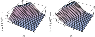
Figure 1: The function $\Psi^{dir}_{0}$ as a function of $x$ and $\Theta$ (y-axis in radians). (a) $n=1$ and (b) $n=2$.

From Fig. 1 we see that for large $x$ the function $\Psi^{dir}_{0}$ peaks in the direction opposite to the sun’s direction of motion , as expected for a M-B distribution. This, however is not true for small $x$. This is understood by observing that $x$ appears explicitly as the coefficient of $\cos{\Theta}$ in the exponential of Eq. (29 ) The situation for the modulated amplitude $H_{m}$ is more complicated since it also depends on the angle $\Phi$. Therefore we will not discuss this case here. We only mention that the modulation here in the case of the $n=2$ is suppressed relative to that for the standard $n=1$ case, independently of the angle of observation. This is expected in view of the results for the standard (non directional) case TET .

III Some applications

In this section we are going to apply the formalism of the previous section in the case of two popular targets: i) The light target ${}^{32}S$ appearing in CS₂ involved in DRIFT DRI and ii) The ¹²⁷I target, which has been employed in the DAMA experiment Bernabei et al (1998, 1996). We will not consider energy thresh hold effects and we will ignore quenching factor effects. We will consider only the coherent mode, but the results obtained for the functions $t,\kappa,h_{m}$ and $\alpha_{m}$ are not expected to be radically modified, if one considers the spin mode.

III.1 The light target CS₂

The nuclear form factor employed was obtained in the shell model description of the target and is shown in Fig. 2.

Figure 2: (a) The form factor $F^{2}(u)$ for ³²S employed in our calculation with $u=Q/Q_{0}$, Q the energy transfer to the nucleus and $Q_{0}=404$ keV. (b) The same quantity a function of the energy transfer $Q$.

The parameter $t$ entering the non directional case is shown in Fig. 3

Figure 3: The quantity $t_{coh}$ is shown for $Q_{min}=0$ with (a) $n=1$ and (b) $n=2$.

We begin our analysis of the directional signal by computing the differential rate with respect to $\xi$, which is used in simulating the experiments DRI ; Green (2002, 2005); Morgan and Green (2005). Our results are presented in Fig. 4 and 5.

Figure 4: The differential rate $dr/d\xi$ for ³²S in as function of $\xi$, the cosine of the angle between the line of observation and the line of recoil. The thick solid, fine solid, short, and long dash correspond to $\Theta=\pi/4,\pi/2,3\pi/4$ and $\pi$ respectively. (a) directional in a given sense for $n=1$ in the case of a WIMP mass of $10$ GeV. (b) The same as in (a) for $n=2$. (c) the same as in (a) for 30 GeV. (d) the same as in (b) for 30 GeV.

Figure 5: The same as in Fig. 4. (a) directional in a given sense for $n=1$ for $100$ GeV. (b) The same as in (a) for $n=2$. (c) the same as in (a) for 250 GeV. (d) the same as in (b) for 250 GeV.

With the above angular distribution we can obtain the average value of $\xi$, $<\xi>$. Thus we get the results shown in Fig. 6.

Figure 6: The quantity $<\xi>$ is shown for $Q_{min}=0$ with (a) $n=1$ and (b) $n=2$. Otherwise the notation is that of Fig. 4

We see that the average value of $\xi$ does not change vary much in going from the $n=1$ to the $n=2$ case. We clearly see that this value is much higher in the case the observation is made opposite to the sun’s direction of motion ($\Theta=\pi$).

We continue our analysis by calculating the parameter $\kappa_{coh}$ discussed above. Our results are shown in Figs 7-10.

Figure 7: The parameter $\kappa$ defined in the text for a light target in the case of a WIMP mass of $10$ GeV. (a) Directional in a given sense for $n=1$. (b) The sum of both senses for $n=1$. (c) The same as in (a) for $n=2$. (d) The same as in (b) for $n=2$.

Figure 8: The same as in Fig. 7 for a WIMP mass of $30$ GeV.

Figure 9: The same as in Fig. 7 for a WIMP mass of $100$ GeV.

Figure 10: The same as in Fig. 7 for a WIMP mass of $250$ GeV.

From these figures we see that in the case of directional experiments the maximum value of $\kappa$ is attained when the observation is made opposite to the sun’s direction of motion. This is expected in the case of the M-B distribution. We have seen above that $<\xi>$ also attains its maximum value. When the sense of direction is not observed the maximum event rate is again attained when the observation is along the line of the sun’s motion.

We will next discus the modulation effect, i.e. the parameters $h_{m}$, shown in Figs 25-28 and $\alpha_{m}$ shown in Figs 15-18. We clearly see that the results depend on the WIMP mass. From the figures 11-14 we see that the modulation for $n=2$ is quite small, reminiscent of a similar result in the case of the non directional case TET . Since the exhibited pattern is otherwise similar to the standard $n=1$ case we will limit our discussion to the $n=1$ case. The modulation amplitude, $h_{m}\approx 0.1$, in the most favored direction $\Theta=\pi$, i.e. opposite to the sun’s direction of motion, is small, but still much larger than that encountered in the non directional case. The absolute maximum $h_{m}\approx 0.4$ seems to occur when $\Phi=\pi$, i.e. inwards towards the center of the galaxy, at an angle $\Theta=0.5\approx\pi/6$. A smaller value of 0.3 is attained when one is looking radially outwards from the center of the galaxy at $\Theta=1.0\approx\pi/3$. Another maximum $h_{m}\approx 0.2$ is attained, when $\Theta\approx\pi/2$, i.e. in a plane perpendicular to the sun’s direction of motion, and $\Phi=\pi/2$, along the line perpendicular to the galactic plane.

When the sense of direction is not observed the modulation picture is quite simple. One sees that the modulation is quite small, when the line of observation is along the sun’s motion and reaches a maximum value, $h_{m}\approx 0.3$ on the plane perpendicular to the sun’s velocity regardless of $\Phi$.

Regarding the phase $\alpha_{m}$ we see that, as expected, it is zero at $\Theta=0$ or $\pi$, reminiscent of the non directional case. For $\Phi=\pi/2$ or $3\pi/2$ this phase is zero for all $\Theta$. This means that in all these cases one has the standard behavior of the modulation (maximum around June 2nd). For $\Phi=0$, outwards from the center of the galaxy, the phase decreases from zero to $\pi/2$ depending so long as $\Theta<0$. During this period the maximum precedes the phase of the Earth. When $\Theta>\pi/2$, it changes sign (the maximum drags behind the phase of the Earth). In other words the maximum occurs in the spring for $\Theta>\pi/2$ and in the autumn for $\Theta<\pi/2$. The opposite is true when $\Phi=\pi$.

In the case when both senses of WIMP recoil are considered the modulation drags behind the phase of the Earth, a maximum in the spring, for $\Phi=0,\pi$ (radially in the galaxy). It attains a maximum in the fall for $\phi=p/2,3\pi/2$ (perpendicular to the plane of the galaxy)

Anyway the above complicated pattern of the shift in the location of the maximum, which depends on the LSP mass, is not expected to cause problems in the analysis of the experiments. The periodic nature of the phenomenon is sufficient.

Figure 11: The parameter $h_{m}$, defined in the text, as function of the polar angle $\Theta$ for a light target in the case of a WIMP mass of $10$ GeV. The fine solid, thick solid, dashed and long dashed curves correspond to $\Phi=0,\pi/2,\pi$, and $3\pi/2$ respectively (the cases $\Phi=\pi/2$ and $3\pi/2$ cannot be distinguished). Note that, when the sense is not distinguished, the maximum angle of the line of observation with the sun’s direction of motion is $\pi/2$, while the maximum azimuthal angle is $\pi$. Now the thick solid, fine solid, dashed and long dashed curve correspond to $\Phi=0,\pi/4,\pi/2$ and $3\pi/4$ respectively (the cases $\Phi=\pi/4$ and $3\pi/4$ cannot be distinguished). (a) The directional rate in a given sense for $n=1$. (b) The sum of both senses is shown for $n=1$. (c) The same as in (a) for $n=2$. (d) the same as in (b) for $n=2$.

Figure 12: The same as in Fig. 11 for a WIMP mass of $30$ GeV.

Figure 13: The same as in Fig. 11 for a WIMP mass of $100$ GeV.

Figure 14: The same as in Fig. 11 for a WIMP mass of $250$ GeV.

Figure 15: The parameter $\alpha_{m}$ (in units of $\pi$), defined in the text, as function of the polar angle $\Theta$ for a light target. Otherwise the notation is the same as in Fig. 11.

Figure 16: The same as in Fig. 15 for a WIMP mass of $30$ GeV.

Figure 17: The same as in Fig. 15 for a WIMP mass of $100$ GeV.

Figure 18: The same as in Fig. 15 for a WIMP mass of $250$ GeV.

III.2 The intermediate mass target ₁₂₇I

The nuclear form factor employed was obtained in the shell model description of the target and is shown in Fig. 19.

Figure 19: (a) The form factor $F^{2}(u)$ for ¹²⁷I employed in our calculation with $u=Q/Q_{0}$, Q the energy transfer to the nucleus and $Q_{0}=64$ keV. (b) The same quantity a function of the energy transfer $Q$.

We first exhibit the previously obtained TET parameter $t_{coh}$ in Fig. 20. We have a suppression as the WIMP mass increases (partly counteracted by the factor $\mu_{r}^{2}/m_{WIMP}$ entering the event rate and not included in $t_{coh}$).

Figure 20: The quantity $t_{coh}$ is shown for $Q_{min}=0$ with (a) $n=1$ and (b) $n=2$.

The behavior of the parameter $\kappa$ is exhibited in Figs 21-24. One can see that for relatively light WIMP in the directional case $\kappa$ has a similar behavior with that encountered above for a light target. It peaks in the direction opposite to the sun’s velocity, i.e at $\Theta=\pi$, as expected. For heavy WIMP masses the maximum value is a factor of 2 smaller than that for a light target and it occurs at lower polar angles $\Theta$. When both senses are considered for $n=1$ $\kappa$ peaks along the sun’s line of motion (by definition here $\Theta=0$). The situation is reversed for heavy WIMP, i.e. it attains a maximum at $\Theta=\pi/2$. This reversed pattern holds for $n=2$, except for very small WIMP masses. Thus, if one could independently establish that the velocity distribution is of M-B type, this signature can be used in constraining the WIMP mass.

Figure 21: The same as in Fig. 7 for the target ¹³²I.

Figure 22: The same as in Fig. 21 for a WIMP mass of $30$ GeV.

Figure 23: The same as in Fig. 21 for a WIMP mass of $100$ GeV.

Figure 24: The same as in Fig. 21 for a WIMP mass of $250$ GeV.

We will next discus the modulation effect, i.e. the parameters $h_{m}$, shown in Figs 25-28. We clearly see that the results depend on the WIMP mass. From the figures 25-28 we see that in the directional case the modulation is similar to that for a light target for small WIMP masses. This is not surprising, since, then, the reduced mass the same for both targets. For heavy WIMPs the modulation $h_{m}$ goes through a small value at around $\Theta=(2/3)\pi$ regardless of the angle $\Phi$. The maximum value of $h_{m}$ is also a bit smaller.

If both senses are counted the modulation amplitude becomes essentially independent of $\Phi$ and attains the maximum value of $h_{m}=0.1-0.3$ depending on the WIMP mass. Note that in this case for heavy WIMPs one has a secondary maximum and a minimum at $\Theta\approx(3/4)\approx\pi/4$, .i.e. when the recoil occurs in the plane perpendicular to the sun’s velocity. Again the absolute maximum occurs at $\Theta=\pi$, i.e. along the sun’s motion.

We will not show the phase $\alpha_{m}$, since the obtained pattern is similar to that encountered for a light target.

Figure 25: The same a in Fig. 11 for the target ¹²⁷I.

Figure 26: The same as in Fig. 25 for a WIMP mass of $30$ GeV.

Figure 27: The same as in Fig. 25 for a WIMP mass of $100$ GeV.

Figure 28: The same as in Fig. 25 for a WIMP mass of $250$ GeV.

Before concluding this section we should mention again that in the case of ¹²⁷I one may have a contribution due to the spin cross section. As we have already mentioned, the controversy regarding the DAMA experiment, employing NaI target, may be attributed to this interaction, which does not enter in experiments involving even nuclear targets. This possibility is currently under study, including our own realistic (static) spin ME and spin form factors. The quantities $t,h,dr/d\xi,\kappa$ and $h_{m}$ do not depend on the spin ME, they only depend on the adopted spin form factors. We do not, however, expect the factors $dr/d\xi,\kappa$ and $h_{m}$, which are the main subject of this work, to be radically different from those presented here for the coherent cross section.

IV Conclusions

We have seen that, given a sufficient number of events, the directional experiments, in which one measures the direction of the nuclear recoil, provide an excellent signature to discriminate against background. Some of these features persist even if the sense of motion of recoils along their line of motion cannot be measured. The predictions depend, of course, on the assumed velocity distribution. In the present work we selected to work with a M-B distribution: (i) the traditional one with characteristic velocity that of sun around the center of the galaxy and (ii) a variant obtained when dark matter is coupled to dark energy via a scalar field yielding an increase in the gravitational field for dark matter TET . In the latter case the characteristic velocity in the WIMP distribution increases by a factor or $n\geq 1$.

In the most favored direction, opposite to the sun’s direction of motion, the event rate is $\approx\frac{1}{2\pi}$ down from the standard non directional experiments. The modulation amplitude in this direction $h_{m}$ depends on the WIMP mass. For a light target it ranges between 0.05 and and 0.1 depending on the WIMP mass. For a heavy target it is somewhat reduced, $h_{m}=0.02-0.07$, but it remains higher than that expected in the non directional experiments. It is also characterized by a definite sign (maximum around June 3nd). Higher values $h_{m}=0.25-0.35$, yielding $50-70\%$ difference between the maximum and the minimum rates, are expected by a judicious choice of the direction of observation. Thus quite large asymmetries with seasonal dependence are predicted. The time of the maximum is also direction dependent, so it cannot be mimicked by seasonal variations of the background.

In partly directional experiments, i.e. experiments in which the sense of motion of the recoiling nucleus is not determined, one no longer can measure asymmetries. We still find, however, that the expected event rate is maximum along the line of motion. Equally large modulation amplitudes $h_{m}$ are predicted with a seasonal variation, which, again, cannot be mimicked by seasonal variations in the background.

The modulation amplitude is decreased, if dark matter is coupled with dark energy, in a fashion analogous to the non directional case. This is not unexpected, since the ratio of the velocity of the earth to the characteristic velocity becomes smaller. This suggests that one should test whether the above conclusions hold, by considering other velocity distributions. Thus one may be able to infer the velocity distribution, when the experimental data become available.

The directional experiments are quite hard. It is encouraging that the angular distribution is such that the average angle is given by $<\xi>=<\cos{\theta}>=0.5-0.8$ depending on the angle $\Theta$, the polar angle of the direction of observation from the sun’s direction of motion. Anyway in experiments planned by DRIFT DRI one can register events recoiling in all directions. If some interesting events are found, one may further analyze them by the direction of recoil to discriminate against background.

V Acknowledgments:

The work of one of the authors (JDV) was completed during a visit to Tuebingen as a Humboldt Research Awardee.

References

-
(1)
S. Hanary et al: Astrophys. J. 545, L5
(2000);
J.H.P Wu et al: Phys. Rev. Lett. 87, 251303 (2001);
M.G. Santos et al: Phys. Rev. Lett. 88, 241302 (2002). -
(2)
P. D. Mauskopf et al: Astrophys. J. 536, L59
(2002);
S. Mosi et al: Prog. Nuc.Part. Phys. 48, 243 (2002);
S. B. Ruhl al, astro-ph/0212229 and references therein. -
(3)
N. W. Halverson et al: Astrophys. J. 568, 38
(2002)
L. S. Sievers et al: astro-ph/0205287 and references therein. - Smoot et al (1992) (COBE Collaboration) G. F. Smoot et al (COBE Collaboration), Astrophys. J. 396, L1 (1992).
- Jaffe et al (2001) A. H. Jaffe et al, Phys. Rev. Lett. 86, 3475 (2001).
- Spergel et al (2003) D. N. Spergel et al, Astrophys. J. Suppl. 148, 175 (2003).
-
(7)
D.N. Spergel et al, Three-Year WMAP Results: Implications
for Cosmology, astro-ph/0603449;
L. Page et al, Three-Year WMAP Results: Polarization Analysis, astro-ph/0603450;
G. Hinsaw et al, Three-Year WMAP Observations: Implications Temperature Analysis, astro-ph/0603451;
N Jarosik et al, Three-Year WMAP Observations: Beam Profiles, Data Processing, Radiometer Characterization and Systematic Error Limits, astro-ph/0603452. - Bennett et al. (1995) D. P. Bennett et al., Phys. Rev. Lett. 74, 2867 (1995).
- Goodman and Witten (1985) M. W. Goodman and E. Witten, Phys. Rev. D 31, 3059 (1985).
- Kosmas and Vergados (1997) T. S. Kosmas and J. D. Vergados, Phys. Rev. D 55, 1752 (1997).
- Ellis and Roszkowski (1992) J. Ellis and L. Roszkowski, Phys. Lett. B 283, 252 (1992).
-
(12)
A. Bottino et al., Phys. Lett B 402, 113
(1997).
R. Arnowitt. and P. Nath, Phys. Rev. Lett. 74, 4592 (1995); Phys. Rev. D 54, 2374 (1996); hep-ph/9902237;
V. A. Bednyakov, H.V. Klapdor-Kleingrothaus and S.G. Kovalenko, Phys. Lett. B 329, 5 (1994). - Vergados (1996) J. D. Vergados, J. of Phys. G 22, 253 (1996).
- (14) M. T. Ressell et al., Phys. Rev. D 48, 5519 (1993); M.T. Ressell and D. J. Dean, Phys. Rev. C 56, 535 (1997).
- Divari et al. (2000) P. C. Divari, T. S. Kosmas, J. D. Vergados, and L. D. Skouras, Phys. Rev. C 61, 054612 (2000).
- Vergados et al. (2005) J. D. Vergados, P. Quentin, and D. Strottman, IJMPE 14, 751 (2005), hep-ph/0310365.
- Vergados and Ejiri (2005) J. D. Vergados and H. Ejiri, Phys. Lett. B 606, 305 (2005), hep-ph/0401151.
- Moustakidis et al. (2005) C. C. Moustakidis, J. D. Vergados, and H. Ejiri, Nucl. Phys. B 727, 406 (2005), hep-ph/0507123.
- (19) H. Ejiri and Ch. C. Moustakidis and J. D. Vergados, Dark matter search by exclusive studies of X-rays following WIMPs nuclear interactions, (to appear in Phys. Lett.); hep-ph/0507123.
-
(20)
The NAIAD experiment B. Ahmed et al, Astropart. Phys. 19 (2003) 691; hep-ex/0301039
B. Morgan, A. M. Green and N. J. C. Spooner, Phys. Rev. D 71 (2005) 103507; astro-ph/0408047. - Shimizu et al. (2003) Y. Shimizu, M. Minoa, and Y. Inoue, Nuc. Instr. Meth. A 496, 347 (2003).
- (22) V.A. Kudryavtsev, Dark matter experiments at Boulby mine, astro-ph/0406126.
- Morgan and Green (2005) B. Morgan and A. M. Green, Phys. Rev. D 72, 123501 (2005).
- Copi et al. (1999) C. Copi, J. Heo, and L. Krauss, Phys. Lett. B 461, 43 (1999).
- Copi and Krauss (2001) C. Copi and L. Krauss, Phys. Rev. D 63, 043507 (2001).
- Vergados (2003) J. D. Vergados, Phys. Rev. D 57, 103003 (2003), hep-ph/0303231.
- Vergados (2004) J. D. Vergados, J.Phys. G 30, 1127 (2004), 0406134.
- Sikivie (1999) P. Sikivie, Phys. Rev. D 60, 063501 (1999).
- Sikivie (1998) P. Sikivie, Phys. Lett. B 432, 139 (1998).
- Vergados (2001) J. D. Vergados, Phys. Rev. D 63, 06351 (2001).
- Green (2001) A. M. Green, Phys. Rev. D 63, 103003 (2001).
- Gelmini and Gondolo (2001) G. Gelmini and P. Gondolo, Phys. Rev. D 64, 123504 (2001).
- Green (2002) A. M. Green, Phys. Rev. D 66, 083003 (2002).
- (34) N. Spooner, Private communication.
- Brouzakis and Tetradis (2006) N. Brouzakis and N. Tetradis, JCAP 0601, 004 (2006).
- (36) N. Tetradis and J.D. Vergados , Detection Rates of Dark Matter Coupled to Dark Energy, to be published; hep-ph/0609078.
- (37) J. D. Vergados, On The Direct Detection of Dark Matter- Exploring all the signatures of the neutralino-nucleus interaction, hep-ph/0601064.
- Green (2005) A. M. Green, Phys. Rev. D 63, 103003 (2005).
- Bernabei et al (1998) R. Bernabei et al, Phys. Lett. B 424, 195 (1998).
- Bernabei et al (1996) R. Bernabei et al, Phys. Lett. B 389, 757 (1996).