Ten years of the Analytic Perturbation Theory in QCD

Abstract

The renormalization group method enables one to improve the properties of the QCD perturbative power series in the ultraviolet region. However, it ultimately leads to the unphysical singularities of observables in the infrared domain. The Analytic Perturbation Theory constitutes the next step of the improvement of perturbative expansions. Specifically, it involves additional analyticity requirement which is based on the causality principle and implemented in the Källen–Lehmann and Jost–Lehmann representations. Eventually, this approach eliminates spurious singularities of the perturbative power series and enhances the stability of the latter with respect to both higher loop corrections and the choice of the renormalization scheme. The paper contains an overview of the basic stages of the development of the Analytic Perturbation Theory in QCD, including its recent applications to the description of hadronic processes.

Keywords: nonanalyticity in $\alpha$, causality, Källen–Lehmann representation

Preamble

The method of the Analytic Perturbation Theory (APT) resolves the problem of unphysical (or ghost) singularities of both the invariant charge of Quantum Chromodynamics (QCD) and the matrix elements of the strong interaction processes. This difficulty (known also as the problem of Moscow zero or Landau pole) first appeared in Quantum Electrodynamics (QED) in the mid-50s of the last century. It played a certain dramatic role in the development of Quantum Field Theory (QFT).

In the late-50s Bogoliubov, Logunov, and Shirkov suggested 1 resolving this problem by merging the renormalization group (RG) method with the Källen–Lehmann representation, which implies the analyticity in the complex $Q^{2}$-variable. The method of APT in QCD is based on the ideas of Ref. 1 .

The development of the APT over the last decade has revealed a number of new principal features of the analytic approach. Specifically, in addition to the resolution of the problem of unphysical singularities, the APT leads to the nonpower functional expansion for QCD observables. The latter possesses an astonishing (in comparison with the perturbative power series) stability with respect to both higher loop corrections and the choice of the renormalization prescription.

I Introduction

The renormalization group method, which was devised in the mid-50s in Ref. 2 (see also paper 3 and the respective chapter of book 4 ), is an inherent part of the contemporary QFT calculations. This method becomes especially useful for singular solutions, when the type of the singularity is affected by perturbative expansion. Besides, the RG method is important for strong interactions, e.g., for QCD.

The QCD description of the majority of hadronic processes requires the use of the RG method. At the same time, the straightforward solutions of the RG equations suffer from the spurious singularities. The one-loop QCD invariant charge $\bar{\alpha}_{\text{{\rm s}}}(Q^{2})$ possesses the ghost pole at $Q^{2}=\Lambda^{2}$, see Eq. (2) below. Higher loop corrections just give rise to additional singularities of the cut type and do not eliminate this problem. The existence of such singularities contradicts the general principles of the local QFT 4 , 5 .

A solution to the problem of the unphysical singularities of the invariant charge was proposed in Ref. 1 . Specifically, this can be achieved by merging the RG method with definite properties of the analyticity in $Q^{2}$-variable. The latter follows from the Källen–Lehmann spectral representation for the transverse Lorentz-invariant amplitude of the dressed photon or boson propagator

$$d(Q^{2})=\frac{1}{\pi}\int_{0}^{\infty}\frac{d\sigma}{\sigma+Q^{2}}\rho(\sigma),$$ (1)

that reflects the basic principles of the local QFT.

In QED, the square of the electron effective charge $\bar{\alpha}(Q^{2})$, which was first introduced by Dirac 6 , is proportional to the transverse amplitude of the dressed photon propagator. The latter satisfies the spectral Källen representation (1), which implies the analyticity in the complex $Q^{2}$-plane with the cut along the negative semiaxis of real $Q^{2}$. The function $\bar{\alpha}(Q^{2})$ is also called the invariant charge or running coupling constant. In accordance with paper 1 , the analytic invariant charge can be reconstructed by making use of the representation (1), the spectral density $\rho(\sigma)$ being defined as the discontinuity of the perturbative QCD invariant charge across the physical cut along the real negative semiaxis $\operatorname{Re}Q^{2}<0$.

The QED analytic invariant charge $\bar{\alpha}$, elaborated in Ref. 1 , possesses the following important properties:

– it has no ghost pole;

– as a function of $\alpha$ it has an essential singularity of the form $\exp(-3\pi/\alpha)$ at the origin;

– for real and positive $\alpha$ it admits a power expansion, that coincides with the perturbative one;

– $\bar{\alpha}$ has finite ultraviolet limiting value $3\pi$, which is independent of the experimental value $\alpha\simeq 1/137$.

In the mid-90s this idea was employed in QCD in Refs. 7 , 8 . Afterwards, the method developed therein was named APT. In QCD, the synthesis of the renormalization invariance with the $Q^{2}$-analyticity has revealed a number of important features of the analytic invariant charge 7 , 8 . In particular, $\alpha_{\text{{\rm E}}}(Q^{2})$ has the universal infrared (IR) stable point. Its value $\alpha_{\text{{\rm E}}}(Q^{2}=0)$ is determined by the one-loop $\beta$-function coefficient $\beta_{0}$. The value $\alpha_{\text{{\rm E}}}(Q^{2}=0)$ is a scheme-independent quantity, since it is not altered by multi-loop corrections. The IR limiting value does not depend on the scale parameter $\Lambda$, which can be evaluated by making use of experimental data. The set of curves $\alpha_{\text{{\rm E}}}(Q^{2})$, corresponding to different values of $\Lambda$, forms a bundle with the common point $\alpha_{\text{{\rm E}}}(0)=1/\beta_{0}$. Therefore, the imposition of the analyticity requirement essentially modifies the IR behavior of the analytic invariant charge.

Another important feature of the analytic approach is that it enables one to define the invariant coupling $\alpha_{\text{{\rm M}}}(s)$ in the timelike (Minkowskian) domain in a self-consistent way 9 . Usually, contemporary QFT calculations involve explicit expressions for observables and other auxiliary RG-invariant (or covariant) quantities, being expressed in terms of the invariant charge. To achieve it, the quantity at hand has first to be represented in an appropriate form. For example, only the quantity defined in the Euclidean region can be expressed in terms of $\bar{\alpha}_{\text{{\rm s}}}(Q^{2})$.

Meanwhile, a number of observables (e.g., the effective cross-sections and quantities related to inclusive decays) are functions of the timelike argument $s=-Q^{2}$, with $s$ being the center-of-mass energy squared. However, in the framework of the RG method, one cannot straightforwardly substitute the spacelike (Euclidean) argument with the timelike (Minkowskian) one. Indeed, in accordance with (1) the amplitudes of propagators, similarly to the transverse photon amplitude $d(Q^{2})$, and the relevant matrix elements acquire complex values for real negative $Q^{2}$ (i.e., for the timelike argument).

Interrelations between the RG-invariant quantities in the Euclidean and Minkowskian domains can only be established by making use of the linear integral transformations. The analytic properties of the invariant charge, which are violated by perturbation theory (PT), and can be recovered within the analytic approach afterwards, play a crucial role here.

Both, the Minkowskian $\alpha_{\text{{\rm M}}}(s)$ and Euclidean $\alpha_{\text{{\rm E}}}(Q^{2})$ charges possess the common IR stable point $\alpha_{\text{{\rm M}}}(s=0)=\alpha_{\text{{\rm E}}}(Q^{2}=0)=1/\beta_{0}$. In the ultraviolet (UV) region these couplings also have the same asymptotic behavior. However, functions $\alpha_{\text{{\rm E}}}(Q^{2})$ and $\alpha_{\text{{\rm M}}}(s)$ cannot be identical in the entire energy range due to certain general arguments 10 .

A key feature of APT is the transformation of series in powers of ${\bar{\alpha}_{\text{{\rm s}}}}$ for observables into the nonpower functional expansions. The latter displays both a milder dependence on the choice of the renormalization scheme and an improved numerical convergence.

Thus, one arrives at the self-consistent method of description of observables. This approach possesses the renormalization invariance and is free of unphysical singularities and related difficulties.

II Analytic perturbation theory

II.1 Singularities of the effective charge

At the one-loop level, the RG summation of the ultraviolet logarithms leads to the singular expression for the QCD running coupling (“invariant charge”)

$$\bar{\alpha}_{\text{{\rm s}}}^{(\ell=1)}(Q^{2})=\frac{\alpha_{\mu}}{1+\alpha_{\mu}\beta_{0}\ln(Q^{2}/\mu^{2})}=\frac{1}{\beta_{0}\ln(Q^{2}/\Lambda^{2})},\qquad\beta_{0}(n_{f})=\frac{11-2n_{f}/3}{4\pi},$$ (2)

where $n_{f}$ denotes the number of active flavors. The scale parameter is defined here in the well-known way, namely $\Lambda=\mu e^{-\frac{1}{2\alpha_{\mu}\beta_{0}}}$.

The function (2) has the IR unphysical singularity at $Q^{2}=\Lambda^{2}$. This problem cannot be solved 11 by taking into account higher-loop corrections. Indeed, the latter just modify the type of singularities, but do not eliminate them. For example, the common form of the two-loop perturbative coupling

$$\bar{\alpha}_{\text{{\rm s}}}^{(2)}(Q^{2})=\frac{1}{\beta_{0}l}\biggl{[}1-\frac{\beta_{1}}{\beta_{0}^{2}}\frac{\ln l}{l}\biggr{]}+O\biggl{(}\frac{\ln^{2}l}{l^{3}}\biggr{)},\qquad l=\ln\frac{Q^{2}}{\Lambda^{2}}$$ (3)

possesses an additional unphysical cut due to the double-log dependence on $Q^{2}$.

A similar situation takes place in QED as well. It is worthwhile to note here that in this latter case unphysical singularities correspond to huge energy scales which have no physical meaning. At the same time, in the case of QCD the value of the parameter $\Lambda$ is about several hundred MeV, that is within the physically-accessible range of energies.

II.2 Analytic approach

In general, the renormalized perturbative expansion can be further modified in a certain way. For example, the Adler function $D(Q^{2})$ is representable by the double series in powers of the running coupling $\alpha_{\mu}$ at a normalization scale $\mu^{2}$ and in powers of $\ln(Q^{2}/\mu^{2})$:

$$D_{\text{{\rm pt}}}\biggl{(}\frac{Q^{2}}{\mu^{2}},\alpha_{\mu}\biggr{)}=\sum_{n}\alpha_{\mu}^{n}\sum_{k=0}^{n}d_{n,k}\ln^{k}\biggl{(}\frac{Q^{2}}{\mu^{2}}\biggr{)}.$$ (4)

In the UV domain this expression is ill-defined due to a large value of logs.

The RG method improves the properties of the perturbative expansion in the UV region by accumulating “large logs” into the invariant charge $\bar{\alpha}_{\text{{\rm s}}}(Q^{2})=\bar{\alpha}_{\text{{\rm s}}}(Q^{2}/\mu^{2},\alpha_{\mu})$. In particular, the RG-improved Adler $D$-function becomes a function of $\bar{\alpha}_{\text{{\rm s}}}$ only, and can be represented by the power series

$$D_{\text{{\rm PT}}}(Q^{2})=D\bigl{(}\bar{\alpha}_{\text{{\rm s}}}(Q^{2})\bigr{)}=\sum_{n}d_{n,0}\bar{\alpha}_{\text{{\rm s}}}^{n}(Q^{2});\qquad\text{{\rm PT}}=\text{{\rm pt}}+\text{{\rm RG}}.$$ (5)

Unlike Eq. (4), the terms of Eq. (5) are $\mu$-independent, and the expansion parameter $\bar{\alpha}_{\text{{\rm s}}}(Q^{2})$ vanishes when $Q^{2}/\mu^{2}\to\infty$, in agreement with the asymptotic freedom.

At the same time, expansion (5) formally remains ill-defined in the IR domain due to unphysical singularities of the expansion parameter $\bar{\alpha}_{\text{{\rm s}}}(Q^{2})$. Thus, on the one hand, the RG improvement of the perturbative series (4) results in a crucial physical property of the asymptotic freedom. On the other hand, an important property of $D$-function, namely, the analyticity in the complex $Q^{2}$-plane with the cut along the negative semiaxis of real $Q^{2}$, is lost in Eq. (5).

The APT method constitutes the next step in the improvement of the perturbative expansion. This method employs the principle of renormalization invariance together with a fundamental principle of causality which is realized in the form of the Källen–Lehmann integral representation (1). In the framework of the APT, the $D$-function can be represented by the nonpower functional expansion

$$D_{\text{{\rm PT}}}(Q^{2})=\sum_{n}d_{n}\bar{\alpha}_{\text{{\rm s}}}^{n}(Q^{2})\quad\to\quad D_{\text{{\rm APT}}}(Q^{2})=\sum_{n}d_{n}{\mathcal{A}}_{n}(Q^{2}).$$ (6)

The Euclidean functions ${\mathcal{A}}_{n}(Q^{2})$ satisfy the Källen–Lehmann representation

$${\mathcal{A}}_{n}(Q^{2})=\frac{1}{\pi}\int_{0}^{\infty}d\sigma\,\frac{\rho_{n}(\sigma)}{\sigma+Q^{2}},$$ (7)

with the spectral function being defined as the discontinuity of the respective power of the invariant charge across the physical cut: $\rho_{k}(\sigma)=\operatorname{Im}\bar{\alpha}_{\text{{\rm s}}}^{k}(-\sigma-i\epsilon)$. The first-order function $\mathcal{A}_{1}(Q^{2})$ corresponds to the analytic running coupling

$$\alpha_{\text{{\rm E}}}(Q^{2})=\frac{1}{\pi}\int_{0}^{\infty}d\sigma\,\frac{\rho(\sigma)}{\sigma+Q^{2}},\qquad\rho(\sigma)\equiv\rho_{1}(\sigma).$$ (8)

The representation (7) determines the analytic properties of the functions ${\mathcal{A}}_{n}(Q^{2})$ in the complex $Q^{2}$-plane. Specifically, these functions (and, therefore, the series (6)), are analytic functions in the complex $Q^{2}$-plane with the cut along the negative semiaxis of real $Q^{2}$. The investigation of the properties of these functions has revealed that the resolution of the ghost pole problem by making use of the APT method eventually leads to the IR stability with respect to higher loop corrections. The results of this investigation are summarized in Table 1 which elucidates the stages of the evolution of the perturbative results: PT $\to$ PT$+$RG $\to$ APT.

Table 1: Properties of various approximations

Method$\int^{b}$	Type of approximation	Properties
		UV	IR	Analyticity
PT$\int$	Double set in powers of
	$\alpha_{\mu}$ and $\ln Q^{2}/\mu^{2}$	$-$	$-$	$+$
PT $+$ RG$\int$	Power series in
	invariant charge $\bar{\alpha}_{\text{{\rm s}}}(Q^{2})$	$+$	$-$	$-$
APT $=$ PT $+$ RG $+$$\int_{a}^{c}$	Nonpower functional expansions
$+$ analyticity	in $\mathcal{A}_{k}(Q^{2})$ and $\mathfrak{A}_{k}(s)$	$+$	$+$	$+$

The last row of the Table contains two sets of functions, namely, $\mathcal{A}_{n}(Q^{2})$ and $\mathfrak{A}_{n}(s)$. The latter appear in the description of the processes depending on the timelike (i.e., Minkowskian) momenta. These functions naturally emerge in the study of the Drell function $R(s)$ which is the ratio of the inclusive hadronic cross-section of the process of the $e^{+}e^{-}$-annihilation to the leptonic one. Here the timelike argument $s$ is the center-of-mass energy squared. The perturbative approximation of $R(s)$ by the power series in the invariant charge, $R_{\text{{\rm PT}}}(s)=\sum_{n}r_{n}\bar{\alpha}_{\text{{\rm s}}}^{n}(s)$, violates the relation between the functions $D(Q^{2})$ and $R(s)$

$$D(Q^{2})=Q^{2}\int_{0}^{\infty}ds\,\frac{R(s)}{(s+Q^{2})^{2}}.$$ (9)

In the framework of the APT, the function $R(s)$ takes the form of the functional expansion

$$R_{\text{{\rm APT}}}=\sum_{n}d_{n}\mathfrak{A}_{n}(s),$$ (10)

with the coefficients $d_{n}$ being identical to those of Eq. (6). The relation between $\mathcal{A}_{k}(Q^{2})$ and $\mathfrak{A}_{k}(s)$

$$\mathcal{A}_{k}(Q^{2})=Q^{2}\int_{0}^{\infty}ds\,\frac{\mathfrak{A}_{k}(s)}{(s+Q^{2})^{2}},$$ (11)

is similar to the relation (9) between $D(Q^{2})$ and $R(s)$. The functions $\mathfrak{A}_{k}$ can also be expressed in terms of the spectral function $\rho_{k}(\sigma)$ 9 :

$$\mathfrak{A}_{k}(s)=\frac{1}{\pi}\int_{\text{{\rm s}}}^{\infty}\frac{d\sigma}{\sigma}\rho_{k}(\sigma).$$ (12)

Figure 1: Euclidean $\alpha_{\text{{\rm E}}}$ and perturbative $\bar{\alpha}_{\text{{\rm s}}}$ charges.

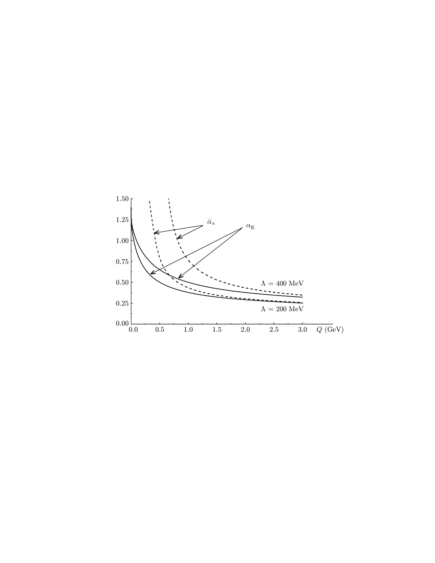
In the leading order the Euclidean running coupling reads 7

$$\alpha_{\text{{\rm E}}}^{(1)}(Q^{2})=\frac{1}{\beta_{0}}\biggl{[}\frac{1}{\ln(Q^{2}/\Lambda^{2})}+\frac{\Lambda^{2}}{\Lambda^{2}-Q^{2}}\biggr{]}.$$ (13)

Figure 1 depicts its behavior for $\Lambda=200$ MeV and $\Lambda=400$ MeV. For comparison, the corresponding perturbative curves are also plotted therein. The enhanced stability of the APT expressions (in comparison with the perturbative ones) is demonstrated in Fig. 2, where the one-loop and two-loop functions are shown. The three-loop analytic running coupling practically coincides with the two-loop one (within the accuracy of 1–2%).

Figure 2: Higher loop stability of the Euclidean charge $\alpha_{\text{{\rm E}}}$.

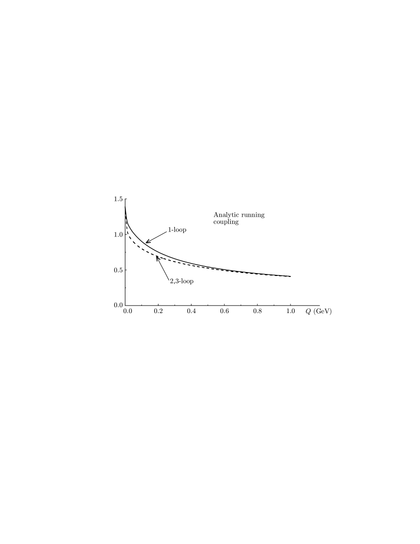
Thus, contrary to the RG-improved perturbation theory, the analyticity, which emerges from the causality, leads to the stabilization of the behavior of the invariant charge in the IR domain. A key property of the approach at hand is that all the expansion functions assume the universal value at $Q^{2}=0$ which eventually results in the stabilization mentioned above. At the same time, the stability in the UV domain (starting from the two-loop level) is due to the asymptotic freedom.

In the framework of the APT the invariant charge in the Minkowskian region can be defined 13 in a self-consistent way as the first of the functions (12):

$$\alpha_{\text{{\rm M}}}(s)=\frac{1}{\pi}\int_{\text{{\rm s}}}^{\infty}\frac{d\sigma}{\sigma}\rho(\sigma),\qquad\rho(\sigma)\equiv\rho_{1}(\sigma).$$ (14)

In the leading order this function reads

$$\alpha_{\text{{\rm M}}}^{(1)}(s)=\frac{1}{\beta_{0}\pi}\arccos\frac{L}{\sqrt{L^{2}+\pi^{2}}}\biggr{|}_{L>0}=\frac{1}{\beta_{0}\pi}\arctan\frac{\pi}{L},\qquad L=\ln\frac{s}{\Lambda^{2}}.$$ (15)

The Euclidean (8) and Minkowskian (14) charges share the same IR limiting value

$$\alpha_{\text{{\rm E}}}(0)=\alpha_{\text{{\rm M}}}(0)=\frac{1}{\beta_{0}},$$ (16)

which is independent of the loop level.

II.3 Higher APT expansion functions

These functions are necessary for the analysis of observables by making use of Eqs. (10) and (6). They satisfy the recurrent relations

$$\frac{1}{k}\frac{d\mathfrak{A}_{k}(s)}{d\ln s}=-\sum_{n\geq 1}\beta_{n-1}\mathfrak{A}_{k+n}(s),\qquad\frac{1}{k}\frac{d\mathcal{A}_{k}(Q^{2})}{d\ln Q^{2}}=-\sum_{n\geq 1}\beta_{n-1}\mathcal{A}_{k+n}(Q^{2}),$$ (17)

which can be employed for their iterative definitions. To achieve it, one has to explicitly solve these relations by making use of additional assumptions of the form $\beta_{\ell\geq\ell_{m}}=0$ and $A_{k\geq K+1}=0$. At the one-loop level ($\beta_{\ell\geq 1}=0$) the APT formulae have a simple and elegant form. In this case, proceeding from the first functions (13) and (15), one can show by making use of relations (17) that

$$\mathcal{A}_{2}^{(1)}(l)=\frac{1}{\beta_{0}^{2}}\biggl{(}\frac{1}{l^{2}}-\frac{e^{l}}{(e^{l}-1)^{2}}\biggr{)}, \mathfrak{A}_{2}^{(1)}(L)=\frac{1}{\beta_{0}^{2}}\frac{1}{L^{2}+\pi^{2}}, l=\ln\biggl{(}\frac{Q^{2}}{\Lambda^{2}}\biggr{)},$$ (18)

$$\mathcal{A}_{3}^{(1)}(l)=\frac{1}{\beta_{0}^{3}}\biggl{(}\frac{1}{l^{3}}-\frac{1}{2}\frac{e^{l}+e^{2l}}{(e^{l}-1)^{3}}\biggr{)}, \mathfrak{A}_{3}^{(1)}(L)=\frac{1}{\beta_{0}^{3}}\frac{L}{(L^{2}+\pi^{2})^{2}}, L=\ln\biggl{(}\frac{s}{\Lambda^{2}}\biggr{)}.$$

The two-loop level is more complicated technically. The point is that the exact solution for $\alpha_{\text{{\rm s}}}$ is expressed in terms of the special Lambert function here, which leads to cumbersome explicit expressions for $\mathcal{A}_{k}$ and $\mathfrak{A}_{k}$ 14 .

Nonetheless, all APT functions obey the following important properties at any loop level:

$\bullet$ Unphysical singularities are absent, no additional parameters being introduced.

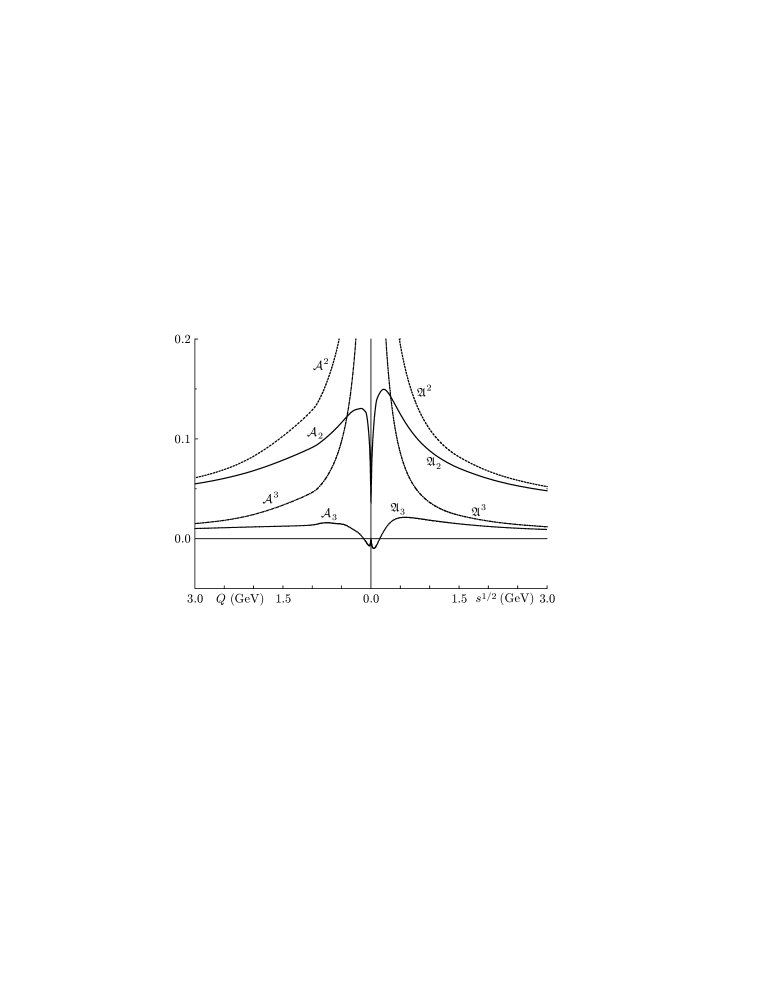
$\bullet$ Higher functions, (18) etc., are not equal to powers of the first ones (13), (15). They oscillate in the vicinity of $|Q^{2}|\sim\Lambda^{2}$ and vanish in the IR limit, see Fig. 3b below. At the same time, these functions tend to the powers of $\alpha_{\text{{\rm s}}}$ in the UV asymptotic.

$\bullet$ The expansions of observables in powers of $\alpha_{\text{{\rm s}}}(Q^{2})$ (for the Euclidean case) and in powers of $\alpha_{\text{{\rm s}}}(s)$ (for the Minkowskian case) are replaced by the expansions over the sets of $\bigl{\{}\mathcal{A}_{k}(Q^{2})\bigr{\}}$ and $\bigl{\{}\mathfrak{A}_{k}(s)\bigr{\}}$, respectively. The latter expansions display a faster convergence with respect to that of the perturbative case.

II.4 Analyticity in the $\alpha_{\text{{\rm s}}}$-plane

As it has been noted above, the expression for the Euclidean coupling $\alpha^{(1)}_{\text{{\rm E}}}(Q^{2}/\mu^{2},\alpha_{\mu})$ contains the nonanalytic term of the form $\exp[-1/\alpha_{\text{{\rm s}}}]$. The latter corresponds to the essential singularity at the origin of the complex $\alpha_{\text{{\rm s}}}$-plane.

More than half a century ago, proceeding from a general reasoning, Dyson argued 15 that such singularity appears in QED inevitably. The explicit form of this singularity coincides with both the term determined in Ref. 16 by merging the renormalization invariance with the causality condition and with the results of Ref. 17 obtained by making use of the functional saddle-point method.

It is worth noting also that the logical inevitability of the nonpower type of the functional APT-expansions was discussed in detail in Refs. 18 .

The conversion of the common QCD running coupling $\alpha_{\text{{\rm s}}}(L)$ into the Euclidean $\alpha_{\text{{\rm E}}}(L)$ or Minkowskian $\alpha_{\text{{\rm M}}}(L)$ one is equivalent to the introduction of a new expansion parameter. It is worth considering two examples

$$\alpha\to w_{1}^{\text{{\rm M}}}(\alpha)=\frac{1}{\pi\beta_{0}}\arccos\frac{1}{\sqrt{1+\pi^{2}\beta_{0}^{2}\alpha^{2}}},\qquad\alpha\to w_{1}^{\text{{\rm E}}}(\alpha)=\alpha+\frac{1}{\beta_{0}}(1-e^{1/(\beta_{0}\alpha)})^{-1}.$$ (19)

The first one is similar to the choice of another renormalization scheme, since the function $w^{\mathrm{M}}(\alpha)$ can be expanded in powers of $\alpha$. The other one transforms into identity in the weak coupling limit, since its second term $e^{-1/(\beta_{0}\alpha)}$ does not contribute to the expansion in powers of $\alpha$ at $\alpha\to 0$.

At the same time, the conversions (19) give rise to the transformations of the invariant charge $\alpha_{\text{{\rm s}}}^{(1)}(L)\to{\mathfrak{A}}_{1}^{(1)}(L)$ and $\alpha_{\text{{\rm s}}}^{(1)}(L)\to\mathcal{A}_{1}^{(1)}(L)$ which are equivalent to Eqs. (13) and (15).

The function $w^{\mathrm{E}}_{1}(\alpha_{\text{{\rm s}}})$ possesses an essential singularity at the origin of the complex $\alpha_{\text{{\rm s}}}$-plane which agrees with the results of Refs. 15 –17 .

Similarly, the sets of higher-order functions of the APT expansions, $\bigl{\{}\mathfrak{A}_{k}(x)\bigr{\}}$, $\bigl{\{}\mathcal{A}_{k}(x)\bigr{\}},\dots$ map onto the nonpower sets $\bigl{\{}w^{\text{{\rm M}}}_{k}(\alpha_{\text{{\rm s}}})\bigr{\}},\bigl{\{}w^{\text{{\rm E}}}_{k}(\alpha_{\text{{\rm s}}})\bigr{\}},\dots$ of the functions:

$$w^{\text{{\rm M}}}_{k}(\alpha_{\text{{\rm s}}})=\mathfrak{A}_{k}\biggl{(}L=\frac{1}{\alpha_{\text{{\rm s}}}}\biggr{)},\qquad w^{\text{{\rm E}}}_{k}(\alpha_{\text{{\rm s}}})=\mathcal{A}_{k}\biggl{(}\frac{1}{\alpha_{\text{{\rm s}}}}\biggr{)},$$ (20)

$$w^{\text{{\rm D}}}_{k}(\alpha_{\text{{\rm s}}})=\aleph_{k}\biggl{(}\ln r^{2}\Lambda^{2}=\frac{1}{\alpha_{\text{{\rm s}}}}\biggr{)},\quad\dots\quad.$$

The adjacent elements satisfy simple differential relations

$$w^{R}_{k+1}(\alpha_{\text{{\rm s}}})=\frac{\alpha_{\text{{\rm s}}}^{2}}{k}\frac{dw^{R}_{k}(\alpha_{\text{{\rm s}}})}{d\alpha_{\text{{\rm s}}}},\qquad R=\text{{\rm E}},\text{{\rm M}},\text{{\rm D}},\dots,$$ (21)

which follow from Eqs. (17) at the one-loop level. Meanwhile, the same-order functions from different sets are interrelated with each other by the integral transformations following from Eq. (11). Besides, all the Euclidean functions $w^{\text{{\rm E}}}_{k}(\alpha)$ possess an essential singularity at $\alpha=0$.

The regularity of the behavior of the timelike APT-invariant charge $\alpha_{\text{{\rm M}}}$ and its effective “powers” $\mathfrak{A}_{k}$ is provided by the summation 20 of an infinite number of perturbative contributions related to the $\pi^{2}$-terms. In turn, the result of the $\pi^{2}$-summation in the Minkowskian region, being extended into the Euclidean domain (11), leads to the recovery of the nonanalytic contributions of the form $\exp\bigl{(}-1/(\beta_{0}\alpha_{\mu})\bigr{)}$ which are “invisible” within the original perturbative expansion. Therefore, the Euclidean functions $\mathcal{A}_{k}$ contain both logarithmic and power terms in $Q^{2}$.

Apparently, the sets of the functions $\bigl{\{}w^{R}_{k}(\alpha_{\text{{\rm s}}})\bigr{\}}$, appearing in the “$\alpha_{\text{{\rm s}}}$-representation”, are similar to Caprini–Fischer sequences 21 which have been obtained proceeding from a different reasoning.

II.5 Global APT and the “distorted” mirror

In the studies of the hadronic processes at various energy scales one has to take into account the dependence of the theoretical results on the active quark flavor number $n_{f}$. Following the Bogoliubov method of massive renormgroup, the algorithm of the smooth matching was devised in Ref. 22 . This algorithm was employed for the analysis of the evolution of the running coupling in the range 3 GeV${}<Q<100$ GeV 23 .

For the massless schemes, the matching of the invariant charge at the “Euclidean thresholds” is commonly employed 24 . However, this procedure destroys the smoothness of the Euclidean function, and, therefore, violates its analyticity.

a

b

Figure 3: a) The global Euclidean and Minkowskian QCD running couplings for $\Lambda^{(3)}=350$ MeV; b) the “distorted mirror” which elucidates the asymmetry of Euclidean and Minkowskian functions.

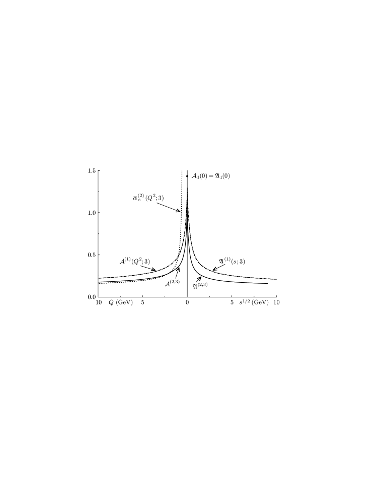
The APT method opens a new opportunity for a self-consistent description of the observables in domains corresponding to various numbers of active quarks $n_{f}$ 25 , 26 . Proceeding from the common matching condition, one defines the spectral functions $\rho(\sigma,n_{f})$ and employs them in Eqs. (7) and (12) afterwards. This procedure provides the analyticity of the Euclidean functions, whereas the Minkowskian functions turn out to be the piecewise smooth ones. Eventually, this results in the “global” APT-functions which “know” about all quark thresholds.

Figure 3a, taken from Ref. 26 , depicts the global APT-charge in the Euclidean and Minkowskian domains. Figure 3b demonstrates the “distorted mirror”, i.e., that the Euclidean and Minkowskian functions possess a similar, but asymmetrical behavior. For comparison with higher functions of the APT-expansions ${\mathcal{A}}_{k}(Q^{2})$ and $\mathfrak{A}_{k}(s)$, the curves corresponding to the powers of the first APT functions are also given therein.

II.6 Possible developments of the minimal APT

As it has already been noted, the present version of the APT contains no additional parameters in comparison with the common RG-improved PT. We call it the minimal one. The straightforward application of the minimal APT in the low energy region (i.e., for the energies of the order of $\Lambda$) is not indisputable. It is worth noting that at such energies the effects due to the quark masses become considerable. In this situation, it is natural to modify the minimal APT by introducing new parameters. It is worthwhile to mention the so-called “synthetic” modification explored in Ref. 27 . Here the running coupling acquires the IR enhancement controlled by an additional parameter. In turn, this allows one to establish a link with the potential quark model. Other variants of the APT involve effective parton masses or modify the spectral representation by shifting the lower integration limit to the two-pion threshold 28 . Besides, there are more formal ways of modification of the minimal APT at low energies 29 .

It is worthwhile to note that for numerical estimations one may employ the results of Ref. 14 which also contains the expressions for the invariant expansion functions in terms of the Lambert function. Since these expansions are rather cumbersome, for practical applications it proves to be convenient to employ simple approximate formulae. A simple explicit expression for the Euclidean QCD function was first proposed in Ref. 30 in the form of a one-parameter model

$${\mathcal{A}}_{\bmod}^{(2)}(Q^{2})=\frac{1}{\beta_{0}}\biggl{[}\frac{1}{l_{2}(a)}+\frac{1}{1-\exp\bigl{(}l_{2}(a)\bigr{)}}\biggr{]}.$$ (22)

This model is based on the one-loop expression with the modified argument

$$l_{2}=l+\frac{\beta_{1}}{2\beta_{0}^{2}}\ln(l^{2}+a\pi^{2}),\qquad l=\ln\frac{Q^{2}}{\Lambda^{2}},$$ (23)

where $a=4$. Recently this model has been essentially developed. It was shown 31 , that the other choice of parameter $a=2$ allows one to approximate both the Euclidean and Minkowskian three-loop APT functions $\mathcal{A}_{k}$, $\mathfrak{A}_{k}$, $k=1,2,3$ within the accuracy sufficient for the description of all the experimental data above 1 GeV. The recurrent relations, modified in a proper way, lead to simple expressions of the “one-loop” form (18) for higher functions. This enables one to employ the new model based on the substitution (23) in the analysis of contemporary experimental data without technical difficulties. This model has been used in the analysis of the inclusive $\Upsilon$-decay in Ref. 31 . It was revealed therein that a weak point of the theoretical processing of rather precise experimental data is the choice of the scale.

III Phenomenological applications

The analytic approach has been successfully employed in studies of many hadronic processes. The literature devoted to the applications of the APT method is rather vast. Below, we mention some important results.

III.1 Inclusive $\tau$-lepton decay

The $\tau$ lepton is the only lepton which is heavy enough to decay into hadrons. Experimental data on the inclusive $\tau$ lepton decay into hadrons possess good accuracy in comparison with those of other hadronic processes. These data constitute a “natural ground” for testing the low-energy QCD.

The importance of the analyticity in the description of the $\tau$ decay can be elucidated by the following example. The experimentally measurable quantity $R_{\tau}$ is related to the life-time of the $\tau$ lepton. The accuracy of its measurement is about 1 %. At the same time, $R_{\tau}$ can be represented as the integral of the imaginary part of the correlation function

$$R_{\tau}=\frac{2}{\pi}\int^{M_{\tau}^{2}}_{0}\frac{ds}{M_{\tau}^{2}}\biggl{(}1-\frac{s}{M_{\tau}^{2}}\biggr{)}^{2}\biggl{(}1+2\frac{s}{M_{\tau}^{2}}\biggr{)}\operatorname{Im}\Pi(s).$$ (24)

The principal difficulty of the theoretical analysis of $R_{\tau}$ is due to the fact that the integration range in Eq. (24) involves the low energy region. Meanwhile, the standard perturbation theory is not valid in the IR domain. Besides, if $\operatorname{Im}\Pi(s)$ is parameterized by the power series in $\bar{\alpha}_{\text{{\rm s}}}$, the integral in Eq. (24) does not exist. This latter difficulty can be avoided by proceeding to the contour integral in the complex $s$-plane

$$R_{\tau}=\frac{1}{2\pi{i}}\oint_{|s|=M_{\tau}^{2}}\frac{ds}{s}\biggl{(}1-\frac{s}{M_{\tau}^{2}}\biggr{)}^{3}\biggl{(}1+\frac{s}{M_{\tau}^{2}}\biggr{)}D(-s),$$ (25)

where $D(-s)$ is the Adler function defined in Eq. (9). However, the original Eq. (24) can be represented in the form of Eq. (25) only if the correlator satisfies the required analytic properties. This latter condition holds in the framework of the APT. The inclusive $\tau$ lepton decay was studied in Refs. 32 , 33 .

III.2 $e^{+}e^{-}$-annihilation into hadrons

The process of $e^{+}e^{-}$-annihilation into hadrons was examined in the framework of the APT in Ref. 34 . The measurable quantity here is $R(s)$ which is the ratio of the hadronic cross-section to the leptonic one. The theoretical analysis of $R(s)$ entails certain complications. The APT results presented below correspond to the so-called “smeared” function $R_{\Delta}(s)$ 35 . The parameter $\Delta$ specifies a minimal “safe” distance from the cut in the complex $s$-plane which guarantees the absence of difficulties of the theoretical description of resonances.

Figure 4: The smeared “experimental” function $R_{\Delta}(q^{2})$ vs. the results of the APT method and the PMS-optimization.

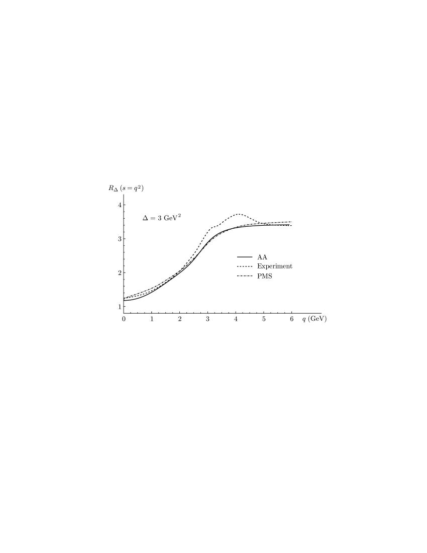
The function $R_{\Delta}(s)$ reads

$$R_{\Delta}(s)=\frac{1}{2i}\bigl{[}\Pi(s+i\Delta)-\Pi(s-i\Delta)\bigr{]},$$ (26)

with $\Delta$ being a finite parameter. By making use of the dispersion relation for $\Pi(q^{2})$, one can express the function (26) in terms of the measurable ratio $R(s)$:

$$R_{\Delta}(s)=\frac{\Delta}{\pi}\int_{0}^{\infty}ds^{\prime}\,\frac{R(s^{\prime})}{(s-s^{\prime})^{2}+\Delta^{2}}.$$ (27)

The function $R(s)$ in the integrand can be approximated by the relevant experimental data at low and intermediate energies and by its perturbative prediction at high energies. This allows one to obtain the “experimental” curve for $R_{\Delta}(s)$. The integration of Eq. (27) results in the smearing of the resonance structure of $R(s)$. The other quantity, which we use in comparing the experimental and theoretical results, is the mentioned-above Euclidean Adler $D$-function. The “experimental” curve for $D(Q^{2})$ can be obtained in the same way as for $R_{\Delta}(s)$.

Figure 5: The “experimental” function $D_{\Delta}(Q^{2})$ vs. the APT results.

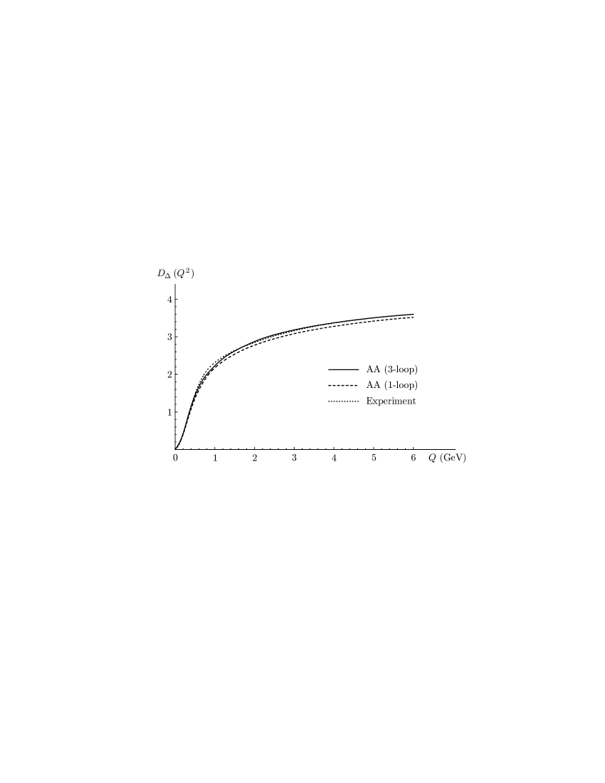
In Figs. 4 and 5, the comparison of the APT results (denoted by the “AA” labels) with the experimental prediction is presented. Figure 4 also shows the curve found with the PMS optimization 36 of the third-order perturbative expansion. The experimental curve is also taken from Ref. 36 . It is worth emphasizing that the APT method and PMS optimization originate in different reasonings, though lead to close numerical results. Further we show that, contrary to perturbation theory, the APT results are practically independent of the subtraction scheme. Therefore, additional optimization of the scheme dependence in APT is not as important as in the perturbative case. The “experimental” curve for $D_{\Delta}$ presented in Fig. 5 is taken from Ref. 37 . Figures 4 and 5 demonstrate good agreement of the theoretical APT results with the “smeared” phenomenological functions $R_{\Delta}$ and $D_{\Delta}$ which have been reconstructed by making use of experimental data on the $e^{+}e^{-}$-annihilation into hadrons.

III.3 Renormalization scheme dependence

An inevitable truncation of perturbative series leads to the well-known problem of the renormalization scheme dependence. It is worth noting that there is no firm criterion of the choice of the renormalization prescription. The partial sum of the perturbative series bears a dependence on the renormalization scheme, which is a source of the theoretical ambiguity in processing the data. In QCD, such ambiguity is the greater the smaller the energy scale is. Therefore, the analysis of the stability of the results should involve the investigation of both higher loop and scheme stability.

The scheme stability of the APT results was first examined in Ref. 38 . In Fig. 6 (taken from Ref. 38 ), the strong correction $r(s)$ to the $R$-ratio of $e^{+}e^{-}$-annihilation into hadrons $R(s)\propto 1+r(s)$ is shown. The curves presented therein were calculated within the APT and PT approaches at the three-loop level. In these calculations the widely-accepted $\overline{\mathrm{MS}}$-scheme and the so-called H-scheme were employed. The latter scheme is close to the former one in the sense of the cancelation index. The issue of the scheme dependence was discussed in detail in Ref. 30 .

Figure 6: The strong correction to the $R$-ratio within the analytic approach (AA) and the standard perturbation theory (PT) for various renormalization schemes.

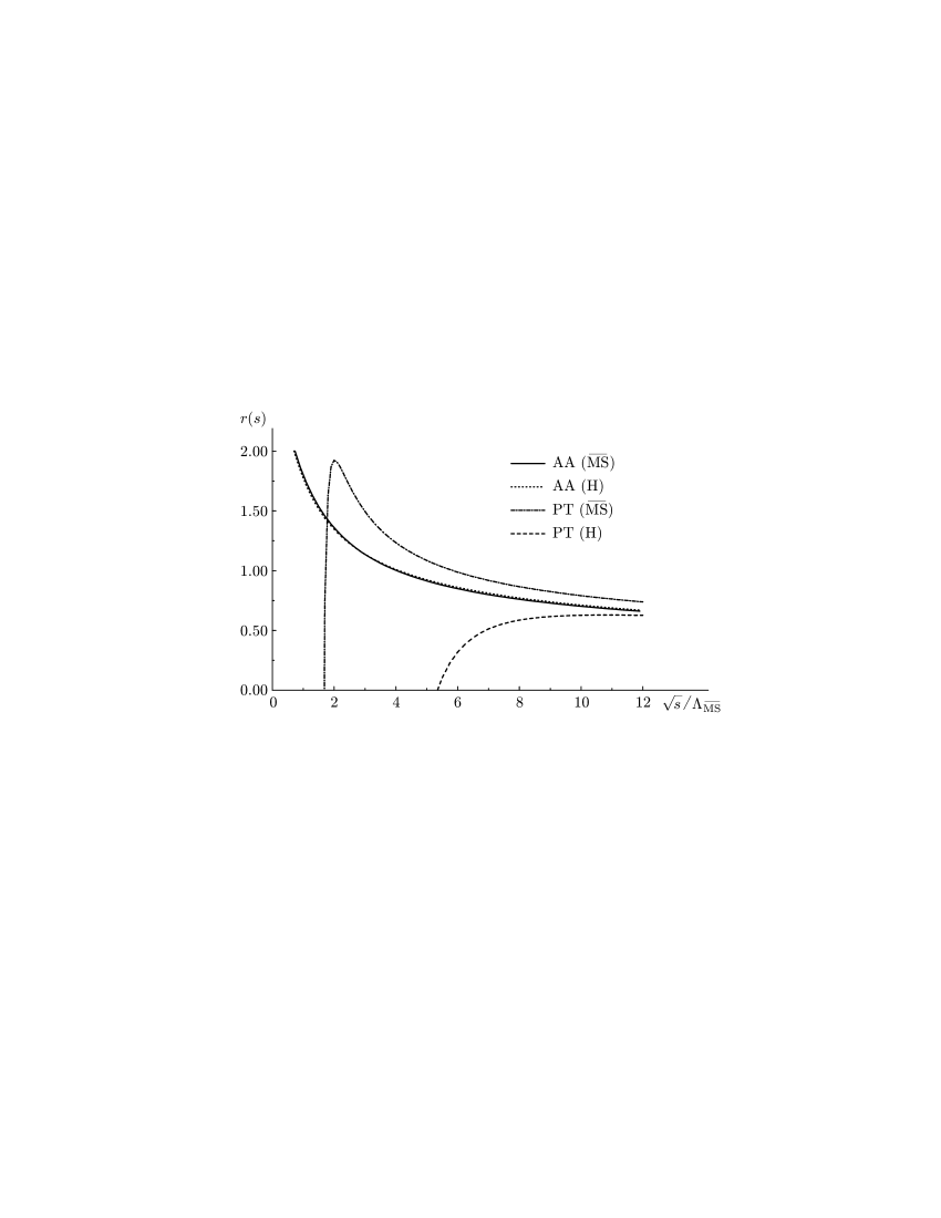
Figure 6 shows that for the energy of about few GeV the standard perturbative approach leads to large ambiguity due to the scheme dependence. The APT method drastically reduces the scheme dependence of the theoretical results. In particular, the APT curves corresponding to different schemes practically coincide. A similar result also takes place for the inclusive $\tau$ lepton decay 33 and for the sum rules of the deep inelastic lepton-hadron scattering 39 .

III.4 Hadronic contribution to the muon anomalous magnetic moment and to the fine structure constant

The APT method has recently been applied 40 to the description of the so-called $R$-related quantities. Among them the hadronic contribution to the muon anomalous magnetic moment plays an important role. The latter quantity (in the leading order in the electromagnetic coupling $\alpha=\alpha_{\text{{\rm QED}}}$) reads

$$a_{\mu}^{\text{{\rm had}}}=\frac{1}{3}\biggl{(}\frac{\alpha}{\pi}\biggr{)}^{2}\int_{0}^{\infty}\frac{ds}{s}K(s)R(s),$$ (28)

with $K(s)$ being a known function.

The hadronic contribution to the fine structure constant $\alpha$ can be represented in the form

$$\Delta\alpha_{\text{{\rm had}}}^{(5)}(s)=-\frac{\alpha}{3\pi}s\>{\mathcal{P}}\!\!\int_{0}^{\infty}\frac{ds^{\prime}}{s^{\prime}}\frac{R(s^{\prime})}{s^{\prime}-s}.$$ (29)

The superscript “(5)” implies that the contributions of only first five quarks ($u$, $d$, $s$, $c$, and $b$) was retained here.

Similar to the case of the $\tau$ decay, the integration range in these expressions includes the low-energy region where the perturbation theory is inapplicable. Quantities (28) and (29) were evaluated in the framework of the APT in Ref. 40 . The latter also employs the assumption about the behavior of the quark mass function at low energy which is based on the nonperturbative solution of the Schwinger–Dyson equation. The obtained theoretical value

$$a_{\mu}^{\text{{\rm had}}}=(698\pm 13)\times 10^{-10}$$ (30)

is in good agreement with the phenomenological estimations of $a_{\mu}^{\text{{\rm had}}}$ which employ the data on $e^{+}e^{-}$-annihilation and $\tau$ decay 41 , 42 .

The hadronic contribution to the fine structure constant at the $Z$-boson scale evaluated in Ref. 40

$$\Delta\alpha_{\text{{\rm had}}}^{(5)}(M_{Z}^{2})=(278.2\pm 3.5)\times 10^{-4}$$ (31)

agrees with the estimation of Ref. 42 which uses the data on $e^{+}e^{-}$-annihilation into hadrons

$$\Delta\alpha_{\text{{\rm had}}}^{(5)}(M_{Z}^{2})=(275.5\pm 1.9_{\text{{\rm expt}}}\pm 1.3_{\text{{\rm rad}}})\times 10^{-4}.$$ (32)

Besides, the method of APT provides a reasonable description of some other quantities, e.g., the inclusive $\tau$ decay characteristic in the vector channel $R_{\tau}^{\text{{\rm V}}}$, and the functions $D_{\Delta}^{\tau}(Q^{2})$ and $R_{\Delta}^{\tau}(s)$ corresponding to the $\tau$ decay data.

III.5 Some other applications

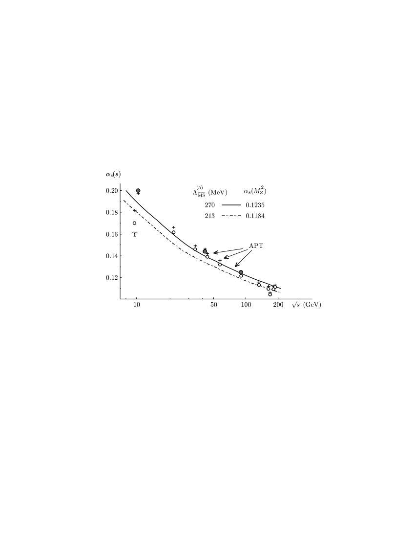
In the framework of the APT the observables in the timelike domain ($s$–channel) can be represented as the nonpower expansion over the functions which retain the so-called $\pi^{2}$-terms. The analysis of the $s$–channel observables 26 has revealed the following. For the energies above $50$ GeV ($n_{f}=5$) the running coupling $\alpha_{\text{{\rm s}}}$ gains the effective positive shift $\Delta{\bar{\alpha}_{\text{{\rm s}}}}\simeq+0.002$ with respect to the standard two-loop (NLO) analysis. In the energy range $10\div 50$ GeV ($n_{f}=5$) the value of this shift increases, namely, $\Delta{\bar{\alpha}_{\text{{\rm s}}}}\simeq+0.003$. This leads to a new value of the QCD invariant charge at the scale of the $Z$-boson mass: $\bar{\alpha}_{\text{{\rm s}}}(M_{Z}^{2})=0.124$. The obtained results are presented in Fig. 7 taken form Ref. 26 .

Figure 7: The analysis of the five-quark timelike domain. The difference between the points denoted by $+$ and $\circ$, $\bullet$ is due to the $\pi^{2}$-corrections. The solid APT curve corresponds to $\Lambda_{\overline{\text{{\rm MS}}}}^{(5)}=270$ MeV and $\alpha_{\text{{\rm s}}}(M_{Z}^{2})=0.124$. The standard dot-dashed curve corresponds to $\Lambda_{\overline{\text{{\rm MS}}}}^{(5)}=213$ MeV and $\alpha_{\text{{\rm s}}}(M_{Z}^{2})=0.118$.

The convergence of the APT expansions is better than that of the perturbative series which is demonstrated in Table 2. The results for the Gross–Llewellyn Smith sum rule for the deep inelastic lepton-hadron scattering at $\sqrt{Q^{2}}\,\sim 1.76$ GeV (Euclidean domain) and for the inclusive $\tau$ lepton decay ($M_{\tau}=1.777$ GeV, timelike region) are given therein. Other applications are presented in Table 2 of Ref. 26 .

Table 2: Various order contributions to observables within PT and APT methods

Process	Method	1st order	2nd order	3rd order
Gross–Llewellyn Smith	PT	65.1%	24.4%	10.5%
sum rule ($\sqrt{Q^{2}}\,\sim 1.76$ GeV)	APT	75.7%	20.7%	3.6%
Inclusive $\tau$ lepton	PT	54.7%	29.5%	15.8%
decay ($M_{\tau}=1.777$ GeV)	APT	87.9%	11.0%	1.1%

It is worthwhile to mention several other applications of APT. The analytic running coupling has been successfully employed in the analysis of the meson spectroscopy 43 . A recent (preliminary) result obtained by the Milano group shows that the form of the QCD interaction extracted from the light quarkonium spectrum as a function of $Q^{2}$ below 1 GeV can be well approximated by the three-loop Euclidean $\alpha_{\text{{\rm E}}}^{(3)}$, the value of the scale parameter $\Lambda$ being close to its world average value.

The Euclidean running coupling and the APT nonpower expansion were employed in the description of the formfactor of the pion-photon transition with Sudakov suppression 44 and the electromagnetic formfactors 45 . Besides, a strong reduction of the sensitivity of the results with respect to both the choice of the factorization scale 46 and the renormalization scheme 47 was revealed.

IV Further development of the APT: the inelastic lepton-hadron scattering

In the previous sections, the APT method has been applied in the analysis of the physical processes which can be described in terms of the two-point function, namely, the correlator of the quark currents. The analyticity condition was employed in the form of the Källen–Lehmann representation. In this section, we address the inelastic lepton-hadron scattering which can be characterized by the structure functions of two scalar arguments. These functions possess rather complicated analytic properties. Nonetheless, the basic idea of the analytic approach turns out to be useful in this case, too.

IV.1 Jost–Lehmann representation

In the case of the inelastic lepton-hadron scattering, the general principles of the axiomatic QFT are accumulated in the Jost–Lehmann (JL) representation 48 for the structure functions. In the nucleon rest frame this representation reads 49

$$W(\nu,Q^{2})=\varepsilon(q_{0})\int d{\mathbf{u}}\,d\lambda^{2}\,\delta\bigl{[}q_{0}^{2}-(M{\mathbf{u}}-{\mathbf{q}})^{2}-\lambda^{2}\bigr{]}\psi({\mathbf{u}},\lambda^{2}),$$ (33)

the support of the distribution $\psi({\mathbf{u}},\lambda^{2})$ being localized on the manifold

$$\rho=|{\mathbf{u}}|\leq 1,\qquad\lambda^{2}\geq\lambda_{\min}^{2}=M^{2}\bigl{(}1-\sqrt{1-\rho^{2}}\,\bigr{)}^{2}.$$ (34)

For the physical process of inelastic scattering the variables $\nu$ and $Q^{2}$ assume positive values. It is convenient to introduce a symmetric in $\nu$ function, to be denoted by the same $W(\nu,Q^{2})$. By making use of the radial symmetry of the distribution $\psi({\mathbf{u}},\lambda^{2})=\psi(\rho,\lambda^{2})$, which follows from the covariance, one can rewrite the JL representation in the covariant form 30

$$W(\nu,Q^{2})=\int_{0}^{1}d\rho\,\rho^{2}\int_{\lambda_{\min}^{2}}^{\infty}d\lambda^{2}\int_{-1}^{1}dz\,\delta\bigl{(}Q^{2}+M^{2}\rho^{2}+\lambda^{2}-2z\rho\sqrt{\nu^{2}+M^{2}Q^{2}}\,\bigr{)}\psi(\rho,\lambda^{2}).$$ (35)

In what follows we adopt the common notation $Q^{2}=-q^{2}$ and $\nu=q{P}$, where $P$ is the hadron momentum and $q$ stands for the momentum transferred.

IV.2 Dispersion relation for the forward scattering amplitude

Proceeding from the representation (35), one can derive the $\nu$-dispersion relation (DR) for the virtual forward Compton scattering amplitude $T(\nu,Q^{2})$

$$T(\nu,Q^{2})=\frac{1}{\pi}\int_{0}^{1}d\rho\,\rho^{2}\int_{\lambda_{\min}^{2}}^{\infty}d\lambda^{2}\int_{-1}^{1}dz\,\frac{\psi(\rho,\lambda^{2})}{Q^{2}+M^{2}\rho^{2}+\lambda^{2}-2z\rho\sqrt{\nu^{2}+M^{2}Q^{2}}-i\epsilon}.$$ (36)

In the complex $\nu^{2}$-plane this function has the cut along the positive semiaxis of real $\nu^{2}$. This cut starts at the point $\nu^{2}_{\min}$ which is determined by

$$\sqrt{\nu^{2}_{\min}+M^{2}Q^{2}}\,=\min_{\{\lambda,\rho,z\}}\biggl{|}\frac{Q^{2}+M^{2}\rho^{2}+\lambda^{2}}{2z\rho}\biggr{|},$$ (37)

that yields $\nu_{\min}={Q^{2}}/{2}$.

Thus, the DR at hand takes the form

$$T(\nu,Q^{2})=\frac{1}{\pi}\int_{Q^{4}/4}^{\infty}\frac{d\nu_{1}^{2}}{\nu_{1}^{2}-\nu^{2}-i\epsilon}W(\nu_{1},Q^{2}).$$ (38)

The DR for the $\nu$-odd structure functions can be derived from the JL representation (33) in a similar way.

In terms of the Bjorken variable $x=Q^{2}/2\nu$ DR (38) takes the form

$$T(\nu,Q^{2})\equiv T(x,Q^{2})=\frac{2}{\pi}\int_{0}^{1}\frac{dx_{1}}{x_{1}}\frac{1}{1-(x_{1}/x)^{2}}W(\nu_{1},Q^{2}).$$ (39)

Thus, $T(x,Q^{2})$ is an analytic function in the complex $x$-plane with the cut along the segment $-1\leq x\leq 1$. The DR (39) is suitable for establishing a link with the operator product expansion (OPE).

A natural scaling variable for the JL representation reads 30 , 51

$$s=\frac{1}{2}\sqrt{\frac{Q^{2}(Q^{2}+4M^{2})}{\nu^{2}+M^{2}Q^{2}}}\,.$$ (40)

In terms of this variable one can represent the dispersion integral (39) in the following form:

$$T(\nu,Q^{2})=\frac{2}{\pi}\int_{0}^{1}\frac{ds_{1}}{s_{1}}\frac{1}{1-(s_{1}/s)^{2}}W(\nu_{1},Q^{2}).$$ (41)

IV.3 Analytic moments of structure functions

For the JL representation a natural scaling variable has the form of Eq. (40). It can also be rewritten in terms of Bjorken variable $x$, namely,

$$s=x\sqrt{\frac{Q^{2}+4M^{2}}{Q^{2}+4M^{2}x^{2}}}\,.$$ (42)

One can infer that for the physical processes the variable $s$ assumes the values in the range between $0$ and $1$.

The variable $s$ differs from both Bjorken and Nachtmann ones, which are commonly employed in the analysis of the deep inelastic scattering. However, it is this variable that leads to the moments which possess appropriate analytic properties.

The $s$-moments of the structure functions can be defined as

$${\mathcal{M}}_{n}(Q^{2})=\frac{1}{{(1+4M^{2}/Q^{2})}^{(n-1)/2}}\int_{0}^{1}ds\,s^{n-2}W(\nu,Q^{2}).$$ (43)

This function can also be rendered in the form of the Källen–Lehmann representation

$${\mathcal{M}}_{n}(Q^{2})=(Q^{2})^{n-1}\int_{0}^{\infty}d\sigma\,\frac{m_{n}(\sigma)}{(\sigma+Q^{2})^{n}},$$ (44)

which elucidates its analytic properties. The support of the weight function $m_{n}(\sigma)$ is located on the semiaxis $\sigma\geq 0$. The function $m_{n}(\sigma)$ can also be represented in terms of the original distribution $\psi(\rho,\sigma)$ of the JL representation.

The analytic moments (43) are related to the $x$-moments $M_{n}(Q^{2})$ by 30

$${\mathcal{M}}_{n}(Q^{2})=\frac{1}{\Gamma\bigl{[}(n+1)/2\bigr{]}}\sum_{k=0}^{\infty}\frac{\Gamma\bigl{[}k+(n+1)/2\bigr{]}}{k!}\biggl{(}-\frac{4M^{2}}{Q^{2}}\biggr{)}^{k}M_{n+2k}(Q^{2}).$$ (45)

In the asymptotic high energy region $x$-, $s$-, and $\xi$-moments coincide with each other, since the power corrections $1/(Q^{2})^{n}$ can be neglected. In the intermediate- and low-energy regions, where higher twist contributions become considerable, one has to distinguish between these moments.

The moments of the structure functions (43), being analytic functions in the complex $Q^{2}$-plane with a cut, are convenient objects for employment within the analytic approach to QCD. The analyticity property is a consequence of the general principles of the local QFT.

IV.4 Relation with the operator product expansion

The identity of the structures of DR in $x$ and $s$ variables allows one to establish a relation of the analytic moments with the operator product expansion. The latter is commonly employed in the study of the $Q^{2}$-evolution of the structure function moments.

The $x$-moments of the structure function correspond to the case when only the Lorentz-structures of the form $P_{\mu_{1}}\dots P_{\mu_{n}}$ are retained in the matrix element

$$\langle P|\widehat{O}_{\mu_{1}\dots\mu_{n}}|P\rangle.$$ (46)

In this case, the OPE for the Compton amplitude leads to the expansion in powers of $(qP)/Q^{2}$, i.e., in the inverse powers of $x$. The same expansion in the inverse powers of $x$ can also be performed in the dispersion integral (39). The relevant coefficients are determined by the $x$-moments. The comparison of these two expansions provides one with the relation of the $x$-moments with the OPE.

In a general case, the symmetric matrix element (46) contains the Lorentz-structures of the form

$$\{P_{\mu_{1}}\dots P_{\mu_{n}}\},\quad M^{2}g_{\mu_{i}\mu_{j}}\{P_{\mu_{1}}\dots P_{\mu_{n-2}}\},\dots\,.$$

The $\xi$-moments correspond to the choice of the operator basis, which involves the traceless tensors (i.e., such that the contraction of the metric $g_{\mu_{i}\mu_{j}}$ with $\langle P|\widehat{O}_{\mu_{1}\dots\mu_{n}}|P\rangle$ over any pair of indices vanishes) as the expansion elements.

The dispersion relation (41) allows one to expand the Compton amplitude in inverse powers of $s$. If the OPE basis is chosen in such a way that an arbitrary contraction of the tensor $\langle P|\widehat{O}_{\mu_{1}\dots\mu_{n}}|P\rangle$ with the nucleon momentum $P_{\mu_{i}}$ vanishes, then the OPE leads to a power series for the forward Compton scattering amplitude with the expansion parameter $q_{\mu}q_{\nu}(P_{\mu}P_{\nu}-g_{\mu\nu}P^{2})(q^{2})^{-2}$ which corresponds to expanding dispersion integral (41) in the inverse powers of $s$. This establishes a relation of the analytic moments of the structure functions with the OPE. It should be stressed that the orthogonality requirement of the symmetric tensor $\langle P|\widehat{O}_{\mu_{1}\dots\mu_{n}}|P\rangle$ to the nucleon momentum $P_{\mu_{i}}$ unambiguously determines its Lorentz structure.

IV.5 Target mass effects

The OPE method was applied to the description of the effects due to the mass of the target in Ref. 52 . This approach leads to the so-called $\xi$-scaling, i.e., the parton distributions become functions of the $\xi$-variable. The resulting expressions for the structure functions are inconsistent with the spectral condition. This situation reminds the ghost pole problem, namely, that an approximate solution contradicts the general principles of the theory.

Figure 8: Ratio of the structure function $F_{3}$, which retains the massive corrections, to the parton distribution for $M^{2}/Q^{2}=1/2$. The solid curve corresponds to the incorporation of the effects due to the target mass by making use of the JL representation. The dashed curve corresponds to the $\xi$-scaling method.

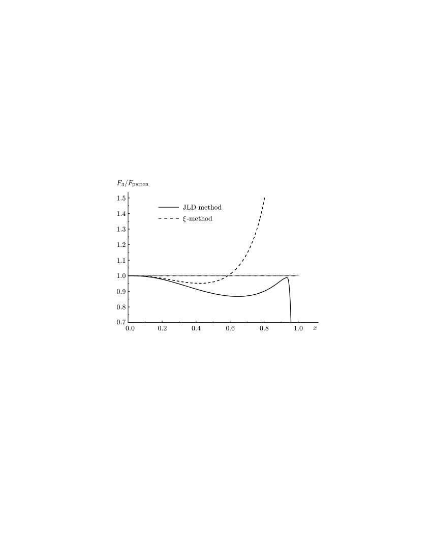
The solution of the spurious singularity problem was based on the Källen–Lehmann representation. One can avoid the contradiction of the issue at hand with the spectral condition by accounting for the target mass corrections in the framework of the JL representation. This approach was implemented in Ref. 53 . Figure 8 depicts the ratio of the structure function $F_{3}$, which retains the mass corrections, to the parton distribution at $M^{2}/Q^{2}=1/2$. The solid curve corresponds to the incorporation of the target mass effects by making use of the JL representation, whereas the dashed one corresponds to the $\xi$-scaling method. One can infer from Fig. 8 that the structure function obtained within the $\xi$-scaling method considerably deviates from that of the JL-method at large values of $x$. It is exactly the region ($x\sim 1$) where the $\xi$-method comes into contradiction with the spectral condition. Since the accuracy of the experimental data is improving and such subtle effects as higher twists become important, in the theoretical studies one should originate in methods which are consistent with the general principles of QFT.

V Conclusion

Renorminvariant PT is a basic tool for investigation of the QFT models as well as for practical calculations of the elementary particle interaction processes. The achievements of PT in QED and in the electroweak theory are well known. The perturbative component of QCD is substantial in the study of practically all the hadronic processes. In the low-energy region, where the nonperturbative effects become essential, the logarithmic contributions calculated within PT are usually supplemented with the power corrections of the nonperturbative origin. Thus, nonperturbative calculations involve PT as a component. As a result, PT affects the determination (from experimental data) of such nonperturbative quantities, as, for example, vacuum expectation values of quark and gluon condensates.

The renormalized perturbative series contains large logarithms. Their presence keeps the terms of the series large at high energies, even when the expansion parameter (i.e., the coupling $\alpha_{\mu}$) is small. Nonetheless, since a perturbative expansion is not the final result of the theory, its certain modification is admissible.

The RG method accumulates large logs within a new expansion parameter, namely, the invariant charge $\bar{\alpha}_{\text{{\rm s}}}(Q^{2})$. This results in perturbative expansions in powers of $\bar{\alpha}_{\text{{\rm s}}}(Q^{2})$. The QCD invariant charge $\bar{\alpha}_{\text{{\rm s}}}(Q^{2})$ is small at high energies, that constitutes a crucial feature of QCD, namely, the asymptotic freedom (i.e., the quark-gluon interaction is suppressed at small distances). Thus, the principle of renorminvariance, which is implemented in the RG method, allows one to modify the perturbative series. The resulting expansions possess reasonable behavior in the UV domain (one has to keep in mind the asymptotic character of the perturbative series). These expansions are suitable for practical applications.

However, at this stage the perturbative expansions entail the problems due to the unphysical singularities of the invariant charge. Such singularities contradict the general principles of the local QFT. The expansion in powers of $\bar{\alpha}_{\text{{\rm s}}}(Q^{2})$ becomes unapplicable at small energies. Besides, at intermediate energies, which are important in QCD applications, the perturbative results contain large ambiguity due to the scheme dependence.

The APT constitutes the next step in the modification of the perturbative expansion which eliminates the afore-mentioned difficulties. Here the principle of renorminvariance is supplemented with the causality principle. In the case of the quark current correlation function the latter principle is implemented in the analyticity condition which corresponds to the spectral Källen–Lehmann representation. For the inelastic lepton-hadron scattering the general properties of structure functions are expressed in the integral Jost–Lehmann representation.

In conclusion, we summarize the most important features of APT:

$\bullet$ The effective Euclidean $\alpha_{\text{{\rm E}}}(Q^{2})$ and Minkowskian $\alpha_{\text{{\rm M}}}(s)$ invariant charges are defined in a self-consistent way; they are free of unphysical singularities; they involve no additional parameters; the higher APT functions $\mathcal{A}_{k}$ and $\mathfrak{A}_{k}$ possess similar properties;

$\bullet$ Euclidean invariant charge $\alpha_{\text{{\rm E}}}$ as a function of $\alpha_{\text{{\rm s}}}$ obeys an essential singularity $\exp(-1/\beta_{0}\alpha_{\text{{\rm s}}})$ at the origin;

$\bullet$ It also has the infrared stable point $\alpha_{\text{{\rm E}}}(0)=\alpha_{\text{{\rm M}}}(0)=1/\beta_{0}$ which is independent of the scale parameter $\Lambda$;

$\bullet$ In the framework of the APT the functional invariant expansions in powers of $\bar{\alpha}_{\text{{\rm s}}}$ for observables are replaced by the nonpower expansions over the sets $\bigl{\{}\mathcal{A}_{k}(Q^{2})\bigr{\}}$ and $\bigl{\{}\mathfrak{A}_{k}(s)\bigr{\}}$;

$\bullet$ The dependence of the APT results on both the multi-loop (NNLO and N³LO) corrections and the choice of the renormalization scheme is drastically suppressed in comparison with that of the perturbative results.

We conclude this paper with the utterance which was the epigraph of one of our papers:

“Take care of Principles and the Principles will take care of you”.

We hope that this sentence is consonant with the creative work of Anatoly Alexeevich Logunov.

Acknowledgements

This work was partially supported by the RFBR grant No. 05-01-00992, Leading scientific schools grant No. NS-5362.2006.2, BelRFBR grant No. F06D-002, and the Collaboration program between the research centers of Belarus and JINR.

References

- (1) N. N. Bogoliubov, A. A. Logunov, and D. V. Shirkov, Zh. Eksp. Teor. Fiz., 1959, 37, 3(9), 805
- (2) N. N. Bogoliubov and D. V. Shirkov, Dokl. Akad. Nauk SSSR, 1955, 103, 391
- (3) N. N. Bogoliubov and D. V. Shirkov, Nuovo Cimento, 1956, 3, 845
- (4) N. N. Bogoliubov and D. V. Shirkov, Introduction to the Theory of Quantum Fields, New York, Wiley, 1959; 1980
-
(5)
N. N. Bogoliubov, A. A. Logunov, and I. T. Todorov, Introduction
to Axiomatic Quantum Field Theory, Benjamin, Reading, MA, 1975;
N. N. Bogoliubov, A. A. Logunov, A. I. Oksak, and I. T. Todorov, General Principles of Quantum Field Theory, Dordrecht, Kluwer, 1990 - (6) P. A. M. Dirac, Theorie du Positron, Structure et Propertiétes des Noyaux Atomiques. Septiéme Conseil du Physique Solvay, Bruxelles, 22–29 October 1933, ed. J. Cockcroft, J. Chadwick, F. Joliot, J. Joliot, N. Bohr, G. Gamov, P. A. M. Dirac, and W. Heisenberg, Paris, Gauthier-Villars, 1934, 203
- (7) D. V. Shirkov and I. L. Solovtsov, JINR Rapid Commun., 1996, 2[76], 5; hep-ph/9604363, 1996
- (8) D. V. Shirkov and I. L. Solovtsov, Phys. Rev. Lett., 1997, 79, 1209; hep-ph/9704333, 1997
- (9) K. A. Milton and I. L. Solovtsov, Phys. Rev. D, 1997, 55, 5295; hep-ph/9611438, 1996
- (10) K. A. Milton and I. L. Solovtsov, Phys. Rev. D, 1999, 59, 107701; hep-th/9812171, 1998
- (11) N. N. Bogoliubov and D. V. Shirkov, Dokl. Akad. Nauk SSSR, 1955, 105, 685
- (12) J. Schwinger, Proc. Natl. Acad. Sci., USA, 1974, 71, 3024; 5047
- (13) K. A. Milton and O. P. Solovtsova, Phys. Rev. D, 1998, 57, 5402; hep-ph/9710316, 1997
(14)
B. A. Magradze, Int. J. Mod. Phys. A, 2000, 15, 2715;
hep-ph/0010070, 2000;
D. S. Kurashev and B. A. Magradze, Theor. Math. Phys., 2003, 135, 531; hep-ph/0104142, 2001 - (15) F. J. Dyson, Phys. Rev., 1952, 85, 631
- (16) D. V. Shirkov, Lett. Math. Phys., 1976, 1, 179; Lett. Nuovo Cim., 1977, 18, 452
(17)
D. V. Shirkov, Theor. Math. Phys., 1979, 40, 785;
D. I. Kazakov and D. V. Shirkov, Fortsch. Phys., 1980, 28, 465 - (18) D. V. Shirkov, Theor. Math. Phys., 1999, 119, 438; hep-th/9810246, 1998; Lett. Math. Phys., 1999, 48, 135
- (19) D. V. Shirkov, Theor. Math. Phys., 2003, 136; hep-ph/0210013, 2002
(20)
A. V. Radyushkin, JINR Rapid Commun., 1996, 78, 96;
hep-ph/9907228, 1999;
N. V. Krasnikov and A. A. Pivovarov, Phys. Lett. B, 1982, 116, 168;
J. D. Bjorken, Two topics in quantum chromodynamics, Particle Physics: Cargèse, 1989, info Proc. Cargèse Summer Inst., Cargèse, France, July 18 – August 4, 1989. NATO Sci. Ser. B, 223, ed. M. Lévy, J. L. Basdevant, M. Jacob, and D. Speiser, New York, Plenum, 1990, 217 - (21) I. Caprini and J. Fischer, Phys. Rev. D, 2000, 62, 054007; Eur. Phys. J. C, 2002, 24, 127; hep-ph/0110344
- (22) D. V. Shirkov, Nucl. Phys. B, 1992, 371, 1,2, 467; Theor. Math. Phys., 1992, 93, 1403
- (23) D. V. Shirkov and S. V. Mikhailov, Z. Phys. C, 1994, 63, 463; hep-ph/9401270, 1994
- (24) W. J. Marciano, Phys. Rev. D, 1984, 29, 580
- (25) D. V. Shirkov, Theor. Math. Phys., 2001, 127, 409; hep-ph/0012283, 2000
- (26) D. V. Shirkov, Eur. Phys. J. C, 2001, 22, 331; hep-ph/0107282, 2001
(27)
A. I. Alekseev and B. A. Arbuzov, Mod. Phys. Lett. A, 1998, 13, 1747; hep-ph/9704228; 2005, A20, 103; hep-ph/0411339;
A. I. Alekseev, Theor. Math. Phys., 2005, 145, 1559 - (28) A. V. Nesterenko and J. Papavassiliou, J. Phys. G, 32, 2006, 1025; hep-ph/0511215
(29)
G. Cvetič, C. Valenzuela, and I. Schmidt, A modification of
minimal analytic QCD at low energies, hep-ph/0508101, 2005;
G. Cvetič and C. Valenzuela, J. Phys. G, 32, 2006, L27; hep-ph/0601050, 2006 - (30) I. L. Solovtsov and D. V. Shirkov, Theor. Math. Phys., 1999, 120, 1220; hep-ph/9909305, 1999
- (31) D. V. Shirkov and A. V. Zayakin, hep-ph/0512325, 2005, to appear in Phys. Atom. Nucl.
(32)
O. P. Solovtsova, JETP Lett., 1996, 64, 714;
K. A. Milton, I. L. Solovtsov, and O. P. Solovtsova, Phys. Lett. B, 1997, 415, 104; hep-ph/9706409, 1997;
O. P. Solovtsova , Theor. Math. Phys., 2003, 134, 365;
K. A. Milton and O. P. Solovtsova, Int. J. Mod. Phys. A, 2002, 17, 26, 3789 - (33) K. A. Milton, I. L. Solovtsov, O. P. Solovtsova, and V. I. Yasnov, Eur. Phys. J. C, 2000, 14, 495; hep-ph/0003030, 2000
(34)
D. V. Shirkov and I. L. Solovtsov, annihilation at low
energies in analytic approach to QCD, Proc. Int. Workshop on
Collisions from to (Novosibirsk,
Russia, March 1–5, 1999), G. V. Fedotovich and S. I. Redin,
Novosibirsk, Russia, Budker Inst. Nucl. Phys., 2000,
122; hep-ph/9906495, 1999;
K. A. Milton, I. L. Solovtsov, and O. P. Solovtsova, Phys. Rev. D, 2001, 64, 016005; hep-ph/0102254, 2001 - (35) E. C. Poggio, H. R. Quinn, and S. Weinberg, Phys. Rev. D, 1976, 13, 1958
- (36) A. C. Mattingly and P. M. Stevenson, Phys. Rev. D, 1994, 49, 437; hep-ph/9307266
- (37) S. Eidelman, F. Jegerlehner, A. L. Kataev, and O. Veretin, Phys. Lett. B, 1999, 454, 369; hep-ph/9812521
- (38) I. L. Solovtsov and D. V. Shirkov, Phys. Lett. B, 1998, 442, 344; hep-ph/9711251, 1997
- (39) K. A. Milton, I. L. Solovtsov, and O. P. Solovtsova, Phys. Lett. B, 1998, 439, 421; hep-ph/9809510, 1998; Phys. Rev. D, 1999, 60, 016001; hep-ph/9809513, 1998
- (40) K. A. Milton, I. L. Solovtsov, and O. P. Solovtsova, Mod. Phys. Lett. A, 2006, 21, 1355; hep-ph/0512209, 2005
(41)
M. Davier, S. Eidelman, A. Höcker, and Z. Zhang, Eur. Phys.
J. C, 2003, 31, 503; hep-ph/0308213;
A. Höcker, The hadronic contribution to the muon g-2, Proc. of 32 Int. Conf. on High-Energy Physics (ICHEP’04) Beijing, China, 16–22 August 2004., Vol. 2, ed. H. Chen, D. Du, W. Li et al, Singapore, World Scientific, 2005, 710; hep-ph/0410081, 2004;
G. W. Bennett, B. Bousquet, H. N. Brown et al, Phys. Rev. Lett., 2004, 92, 161802; hep-ex/0401008;
A. Czarnecki, Nucl. Phys. B (Proc. Suppl.), 2005, 144, 201 - (42) K. Hagiwara, A. D. Martin, D. Nomura, and T. Teubner, Phys. Rev. D, 2004, 69, 093003; hep-ph/0312250
- (43) M. Baldicchi and G. M. Prosperi, Phys. Rev. D, 2002, 66, 074088; hep-ph/0202172, 2002; AIP Conf. Proc., 2005, 756, 152; hep-ph/0412359, 2004
- (44) N. G. Stefanis, W. Schroers, and Hyun-Chul Kim, Eur. Phys. J. C, 2000, 18, 137; hep-ph/0005218
- (45) A. P. Bakulev, K. Passek-Kumericki, W. Schroers, and N. G. Stefanis, Phys. Rev. D, 2004, 70, 033014; hep-ph/0405062, 2004
- (46) A. P. Bakulev, A. I. Karanikas, and N. G. Stefanis, Phys. Rev. D, 2005, 72, 074015; hep-ph/0504275, 2005
- (47) N. G. Stefanis, A. P. Bakulev, A. I. Karanikas, and S. V. Mikhailov, Fractional analytic perturbation theory in QCD and exclusive reaction, hep-ph/0601270, 2006
- (48) R. Jost and H. Lehmann, Nuovo Cimento, 1957, 5, 1598
- (49) N. N. Bogoliubov, V. S. Vladimirov, and A. N. Tavkhelidze, Theor. Math. Phys., 1972, 12, 839
- (50) N. N. Bogoliubov and D. V. Shirkov, Dokl. Akad. Nauk SSSR, 1957, 113, 529
- (51) B. Geyer, D. Robaschik, and E. Wieczorek, Fortschr. Phys., 1979, 27, 75; Sov. J. Part. Nucl., 1980, 11, 52
- (52) H. Georgi and H. D. Politzer, Phys. Rev. D, 1976, 14, 1829
- (53) I. L. Solovtsov, Part. Nucl. Lett., 2000, 4[101], 10