FTUAM 06-17

IFT-UAM/CSIC 06-54

LPT-ORSAY-06-69

hep-ph/0611232

Towards constraints on the SUSY seesaw
from flavour-dependent leptogenesis

S. Antusch^a and A. M. Teixeira^a,b

^a Departamento de Física Teórica C-XI and

Instituto de Física Teórica C-XVI,
Universidad Autónoma de Madrid, Cantoblanco, E-28049 Madrid, Spain

^b Laboratoire de Physique Théorique

Université de Paris-Sud XI,
Bâtiment 201, F-91405 Orsay Cedex, France

We systematically investigate constraints on the parameters of the supersymmetric type-I seesaw mechanism from the requirement of successful thermal leptogenesis in the presence of upper bounds on the reheat temperature $T_{\mathrm{RH}}$ of the early Universe. To this end, we solve the flavour-dependent Boltzmann equations in the MSSM, extended to include reheating. With conservative bounds on $T_{\mathrm{RH}}$, leading to mildly constrained scenarios for thermal leptogenesis, compatibility with observation can be obtained for extensive new regions of the parameter space, due to flavour-dependent effects. On the other hand, focusing on (normal) hierarchical light and heavy neutrinos, the hypothesis that there is no CP violation associated with the right-handed neutrino sector, and that leptogenesis exclusively arises from the CP-violating phases of the $U_{\text{MNS}}$ matrix, is only marginally consistent. Taking into account stricter bounds on $T_{\mathrm{RH}}$ further suggests that (additional) sources of CP violation must arise from the right-handed neutrino sector, further implying stronger constraints for the right-handed neutrino parameters.

1 Introduction

One of the most appealing mechanisms to generate the observed baryon asymmetry of the Universe (BAU), $n_{\mathrm{B}}/n_{\gamma}\,\approx\,(6.10\,\pm\,0.21)\,\times\,10^{-10}$ [1], is that of baryogenesis via leptogenesis. Thermal leptogenesis is an attractive and minimal mechanism, in which a lepton asymmetry is dynamically generated, and then converted into a baryon asymmetry due to $(B+L)$-violating sphaleron interactions [2]. The latter exist both in the Standard Model (SM) and in its minimal supersymmetric (SUSY) extension, the MSSM.

The seesaw mechanism [3, 4] provides an elegant explanation for the observed smallness of the neutrino masses and, in addition, it offers the possibility of leptogenesis [5]. In this case, the lepton asymmetry is generated by the out-of-equilibrium decays of the same heavy right-handed neutrinos which are responsible for the suppression of the light neutrino masses. In spite of being one of the most simple frameworks where thermal leptogenesis can be realised, the seesaw mechanism introduces a large number of new parameters (in both its SM and MSSM versions). Although an important amount of data has already been collected, many of the seesaw parameters, namely those associated with the right-handed neutrino sector, are experimentally unreachable. As discussed by many authors, strong constraints on the seesaw parameter space can be imposed from the requirement of successful thermal leptogenesis [6]. Typically, all these studies relied on the so-called flavour-independent (or one-flavour) approximation to thermal leptogenesis. In the latter approximation, the baryon asymmetry is calculated by solving a Boltzmann equation for the abundance of the lightest right-handed neutrino, and for the total lepton asymmetry. Additionally, in the flavour-independent approximation, the only relevant CP violation sources are those associated with the right-handed neutrino sector (more concretely, the complex $R$-matrix angles, when working in the so-called Casas-Ibarra parameterisation [7]).

In recent years, the impact of flavour in thermal leptogenesis has merited increasing attention [8]-[16]. In fact, the one-flavour approximation is only rigorously correct when the interactions mediated by the charged lepton Yukawa couplings are out of equilibrium. Below a given temperature (e.g. $\mathcal{O}(10^{12}\,\text{GeV})$ in the SM), the tau Yukawa coupling comes into equilibrium (later followed by the couplings of the muon and electron). Flavour effects are then physical and become manifest, not only at the level of the generated CP asymmetries, but also regarding the washout processes that destroy the asymmetries created for each flavour. In the full computation, the asymmetries in each distinguishable flavour are differently washed out, and appear with distinct weights in the final baryon asymmetry.

Flavour-dependent leptogenesis has recently been addressed in detail by several authors [10]-[14]. In particular, flavour-dependent effects in leptogenesis have been studied, and shown to be relevant, in the two right-handed neutrino models [12] as well as in classes of neutrino mass models with three right-handed neutrinos [14]. The quantum oscillations/correlations of the asymmetries in lepton flavour space have been included in Ref. [10] and the treatment has also been generalised to the MSSM [14].

One interesting implication of the flavour-dependent treatment is that in addition to the right-handed sector CP violating phases (that is, a complex $R$-matrix), low-energy CP violating sources, associated with the light neutrino sector, also play a relevant role. Even in the absence of CP violation from the right-handed neutrino sector (which would lead to a zero baryon asymmetry in the one-flavour approximation), a non-vanishing baryon asymmetry can in principle be generated from the CP phases in the Maki-Nakagawa-Sakata matrix, $U_{\text{MNS}}$. Strong connections between the low-energy CP phases of the $U_{\text{MNS}}$ matrix and CP violation for flavour-dependent leptogenesis can either emerge in classes of neutrino mass models [14] or under the hypothesis of no CP violation sources associated with the right-handed neutrino sector (real $R$) [13, 15, 16]. In addition, in the latter limit, bounds on the masses of the light and heavy neutrinos and on the flavour-dependent decay asymmetries have been derived [16]. The correlation of the baryon asymmetry with the effective Majorana mass in neutrinoless double beta ($0\nu\beta\beta$) decays has also been addressed [15]. Another appealing aspect of the flavour-dependent treatment is that at least one of the CP sources, the Dirac CP-violating phase, is likely to be experimentally measured (one of the Majorana phases could also in principle be measured - even though this represents a considerable challenge [17], while the right-handed phases are experimentally unaccessible).

In the supersymmetric implementation of the seesaw mechanism, further constraints on the seesaw parameter space can arise. These are particularly relevant in models of local SUSY (i.e. supergravity). First, one should consider cosmological bounds on the reheat temperature ($T_{\text{RH}}$) after inflation, associated with the thermal production of gravitinos. $T_{\text{RH}}$ has generally a strong impact on thermal leptogenesis, since the production of right-handed neutrinos is suppressed if their mass largely exceeds $T_{\text{RH}}$. In fact, due these bounds on the reheat temperature, viable thermal leptogenesis will impose strong constraints on the seesaw parameter space of locally supersymmetric models. Secondly, additional bounds on the SUSY seesaw parameter space arise from low-energy observables, namely lepton flavour violating (LFV) muon and tau decays such as $l_{j}\to l_{i}\,\gamma$ and $l_{j}\to 3\,l_{i}$ ($i<j$), and charged lepton electric dipole moments. In studies of LFV, thermal leptogenesis in the flavour-independent approximation has been discussed in Ref. [18], and reheating effects have been explicitly included in Ref. [19]. With a potential future observation of the sparticle spectrum, the combined constraints on the SUSY seesaw parameters from leptogenesis and LFV could lead to interesting information on the heavy neutrino sector, which is otherwise unobservable at accelerators.

In this study, our aim is to investigate the constraints on the parameters of the type-I SUSY seesaw mechanism from the requirement of a successful flavour-dependent thermal leptogenesis in the presence of upper bounds on the reheat temperature of the early Universe. Previous studies of flavour-dependent thermal leptogenesis were conducted in the SM, and for a mass range of the lightest right-handed neutrino where only the tau-flavour is in thermal equilibrium. In the present analysis, we will work in the context of the MSSM extended by three right-handed neutrino superfields. Moreover, for the temperatures we will consider, both tau- and muon-flavours are in thermal equilibrium, so that in fact all leptonic flavours must be treated separately. We update the Boltzmann equations of Ref. [20] to include flavour effects, and point out which regions of the seesaw parameter space generically enable optimal efficiency and/or optimal decay asymmetries for leptogenesis (focusing on the case of hierarchical light and heavy neutrino masses). We then discuss the differences between the flavour-independent approximation and the correct flavour-dependent treatment. We encounter interesting new regions of the seesaw parameter space, which are now viable due to flavour-dependent effects. On the other hand, and as we will discuss throughout this work, scenarios of leptogenesis solely arising from the $U_{\text{MNS}}$ phases are quite difficult to accommodate, and become increasingly disfavoured when stronger bounds on $T_{\text{RH}}$ are taken into account.

In the presence of strict bounds on $T_{\text{RH}}$, whether or not it is possible to generate the observed baryon asymmetry exclusively from low-energy Dirac and/or Majorana phases is still a question that deserves careful consideration. Likewise, it is worth considering to which extent right-handed sector phases (other than those of the $U_{\text{MNS}}$) could affect a potentially viable scenario of low-energy CP violating leptogenesis, and vice-versa.

Our work is organised as follows. In Section 2, we briefly summarise the most relevant aspects of the type-I SUSY seesaw mechanism. Section 3 is devoted to the discussion of thermal leptogenesis with reheating. In addition to estimating the baryon asymmetry, we focus on the constraints on the reheat temperature arising from the gravitino problem. A short summary of the limitations and approximations of our computation is also included. In Section 4, we finally discuss the constraints on the seesaw parameters obtained from the requirement of successful leptogenesis, namely constraints on the neutrino masses and on the $R$-matrix mixing angles. Our conclusions are presented in Section 5.

2 The seesaw mechanism and its parameters

In what follows, we briefly introduce the most relevant features of neutrino mass generation via the seesaw mechanism. In the MSSM extended by three right-handed neutrino superfields, the relevant terms in the superpotential to describe a type-I SUSY seesaw are

$$W\,=\,\hat{N}^{c}\,\lambda_{\nu}\,\hat{L}\,\hat{H}_{2}\,+\,\hat{E}^{c}\,\lambda_{\ell}\,\hat{L}\,\hat{H}_{1}\,+\,\frac{1}{2}\,\hat{N}^{c}\,m_{M}\,\hat{N}^{c}\,.$$ (1)

In the above, $\hat{N}^{c}$ denotes the additional superfields containing the right-handed neutrinos $N_{i}$ and sneutrinos $\widetilde{N}_{i}$. The lepton Yukawa couplings $\lambda_{\ell,\nu}$ and the Majorana mass $m_{M}$ are $3\times 3$ matrices in lepton flavour space. From now on, we will assume that we are in a basis where $\lambda_{\ell}$ and $m_{M}$ are diagonal. After electroweak (EW) symmetry breaking, the charged lepton and Dirac neutrino mass matrices can be explicitly written as $m_{\ell}\,=\,\lambda_{\ell}\,\,v_{1}$, $m_{D}\,=\,\lambda_{\nu}\,v_{2}$, where $v_{i}$ are the vacuum expectation values (VEVs) of the neutral Higgs scalars, with $v_{1(2)}=\,v\,\cos(\sin)\beta$ and $v=174$ GeV.

The $6\times 6$ neutrino mass matrix, whose eigenvalues are the masses of the six Majorana neutrinos, is given by

$$M^{\nu}\,=\,\left(\begin{array}[]{cc}0&\lambda^{T}_{\nu}\,v_{2}\\ \lambda_{\nu}\,v_{2}&m_{M}\end{array}\right)\,.$$ (2)

In the seesaw limit, $m_{M_{i}}\,\gg\,v_{2}$, one obtains three light and three heavy states, $\nu_{i}$ and $N_{i}$, respectively. Block-diagonalisation of the neutrino mass matrix of Eq. (2), leads (at lowest order in the $(\lambda_{\nu}\,v_{2}/m_{M})^{n}$ expansion) to the standard seesaw equation for the light neutrino mass matrix,

$$m_{\nu}\,=\,-v_{2}^{2}\,\lambda_{\nu}^{T}\,m_{M}^{-1}\,\lambda_{\nu}\,,$$ (3)

and to $m_{N}\,\simeq\,m_{M}$. Since we are working in a basis where $m_{M}$ is diagonal, the heavy eigenstates are then given by

$$m_{N}\,=\,m_{N}^{\text{diag}}\,=\,\text{diag}\,(m_{N_{1}},m_{N_{2}},m_{N_{3}})\,.$$ (4)

The matrix $m_{\nu}$ can be diagonalised by the unitary matrix $U_{\text{MNS}}$, leading to the following masses for the light physical states

$$U_{\text{MNS}}^{T}\,m_{\nu}\,U_{\text{MNS}}\,=\,m_{\nu}^{\text{diag}}\,=\,\text{diag}\,(m_{\nu_{1}},m_{\nu_{2}},m_{\nu_{3}})\,.$$ (5)

Here we will use the standard parameterisation for the $U_{\mathrm{MNS}}$, given by

$$U_{\text{MNS}}=\left(\begin{array}[]{ccc}c_{12}\,c_{13}&s_{12}\,c_{13}&s_{13}\,e^{-i\delta}\\ -s_{12}\,c_{23}\,-\,c_{12}\,s_{23}\,s_{13}\,e^{i\delta}&c_{12}\,c_{23}\,-\,s_{12}\,s_{23}\,s_{13}\,e^{i\delta}&s_{23}\,c_{13}\\ s_{12}\,s_{23}\,-\,c_{12}\,c_{23}\,s_{13}\,e^{i\delta}&-c_{12}\,s_{23}\,-\,s_{12}\,c_{23}\,s_{13}\,e^{i\delta}&c_{23}\,c_{13}\end{array}\right)\,.\,P\,,$$ (6)

with $P\,=\,\text{diag}\,(e^{-i\frac{\varphi_{1}}{2}},e^{-i\frac{\varphi_{2}}{2}},1)$, and where $c_{ij}\equiv\cos\theta_{ij}$, $s_{ij}\equiv\sin\theta_{ij}$. The parameters $\theta_{ij}$ are the neutrino flavour mixing angles, $\delta$ is the Dirac phase and $\varphi_{1,2}$ are the Majorana phases.

In view of the above, the seesaw equation, Eq. (3), can be solved for the neutrino Yukawa coupling $\lambda_{\nu}$ using the Casas-Ibarra parameterisation [7] as

$$\lambda_{\nu}\,v_{2}\,=\,i\,\sqrt{m^{\text{diag}}_{N}}\,R\,\sqrt{m^{\text{diag}}_{\nu}}\,U^{\dagger}_{\text{MNS}}\,,$$ (7)

where $R$ is a generic complex orthogonal $3\times 3$ matrix that encodes the possible extra neutrino mixings (associated with the right-handed sector) in addition to those in the $U_{\text{MNS}}$. $R$ can be parameterised in terms of three complex angles, $\theta_{i}$ $(i=1,2,3)$ as

$$R\,=\,\left(\begin{array}[]{ccc}c_{2}\,c_{3}&-c_{1}\,s_{3}\,-\,s_{1}\,s_{2}\,c_{3}&s_{1}\,s_{3}\,-\,c_{1}\,s_{2}\,c_{3}\\ c_{2}\,s_{3}&c_{1}\,c_{3}\,-\,s_{1}\,s_{2}\,s_{3}&-s_{1}\,c_{3}\,-\,c_{1}\,s_{2}\,s_{3}\\ s_{2}&s_{1}\,c_{2}&c_{1}\,c_{2}\end{array}\right)\,,$$ (8)

with $c_{i}\equiv\cos\theta_{i}$, $s_{i}\equiv\sin\theta_{i}$. Eq. (7) is a convenient means of parameterising our ignorance of the full neutrino Yukawa couplings, while at the same time allowing to accommodate the experimental data. Notice that it is only valid at the right-handed neutrino scales $m_{M}$, so that the quantities appearing in Eq. (7) are the renormalised ones, $m^{\text{diag}}_{\nu}\,(m_{M})$ and $U_{\text{MNS}}\,(m_{M})$.

In this study, we shall mainly focus on the simplest scenario, where both heavy and light neutrinos are hierarchical, $m_{N_{1}}\,\ll\,m_{N_{2}}\,\ll\,m_{N_{3}}$ and $m_{\nu_{1}}\,\ll\,m_{\nu_{2}}\,\ll\,m_{\nu_{3}}$, and in particular, we will assume a normal ordering of the light neutrinos. Thus, the masses $m_{\nu_{2,3}}$ can be written in terms of the lightest mass $m_{\nu_{1}}$ and the solar/atmospheric mass-squared differences as $m_{\nu_{2}}^{2}\,=\,\Delta m_{\text{sol}}^{2}\,+\,m_{\nu_{1}}^{2}$ and $m_{\nu_{3}}^{2}\,=\,\Delta m_{\text{atm}}^{2}\,+\,m_{\nu_{1}}^{2}$.

In summary, when working in the $R$-matrix parameterisation, the 18 parameters of the seesaw mechanism are accounted by the three heavy neutrinos masses, $m_{N_{i}}$, the mass of the lightest neutrino $m_{\nu_{1}}$ plus the two mass squared differences $\Delta m_{\text{sol}}^{2}$ and $\Delta m_{\text{atm}}^{2}$, the three mixing angles $\theta_{ij}$ and three CP violating phases $\delta,\varphi_{1},\varphi_{2}$ of the $U_{\text{MNS}}$ matrix, and the three complex angles $\theta_{i}$ of the matrix $R$. As mentioned in the Introduction, many of the latter parameters, namely those associated with the heavy neutrino sector, are experimentally unreachable. Nevertheless, it is possible to derive interesting bounds from the requirement of successful thermal leptogenesis, and we proceed to do so in the following sections.

3 Flavour-dependent thermal leptogenesis with
reheating

As recently pointed out [10, 11, 12], flavour can have a strong impact in baryogenesis via thermal leptogenesis. The effects are manifest not only in the flavour-dependent CP asymmetries, but also in the flavour-dependence of scattering processes in the thermal bath, which can destroy a previously produced asymmetry. In fact, depending on the temperatures at which thermal leptogenesis takes place, and thus on which interactions mediated by the charged lepton Yukawa couplings are in thermal equilibrium, flavour-dependent effects can have a strong impact on the estimation of the produced baryon asymmetry [8]-[16]. For example, in the MSSM, for temperatures between circa $(1+\tan^{2}\beta)\times 10^{5}\>\mbox{GeV}$ and $(1+\tan^{2}\beta)\times 10^{9}\>\mbox{GeV}$, the $\mu$ and $\tau$ Yukawa couplings are in thermal equilibrium and all flavours in the Boltzmann equations are to be treated separately. For instance, for $\tan\beta=30$, this applies for temperatures below about $10^{12}$ GeV (and above $10^{8}\>\mbox{GeV}$), a temperature range we will be subsequently considering. Moreover, in the full flavour-dependent treatment, lepton asymmetries are generated in each individual lepton flavour. Processes which can wash out these asymmetries are also flavour-dependent, i.e. the inverse decays from electrons can only destroy the lepton asymmetry in the electron flavour. We will address the latter issues in Section 3.1.

In thermal leptogenesis, the population of right-handed neutrinos $N_{1}$ is produced from scattering processes in the thermal bath. To generate the observed baryon asymmetry comparatively high temperatures of the early Universe are required, and these should not lie much below the mass of the lightest right-handed neutrino, $m_{N_{1}}$. Even under optimal conditions, thermal leptogenesis demands $m_{N_{1}}\gtrsim 10^{9}$ GeV (for hierarchical light and heavy neutrinos) [21]. High temperatures compatible with thermal leptogenesis can arise in the process of reheating which takes place after cosmic inflation [22]. The temperature of the Universe at the end of reheating is referred to as the reheat temperature $T_{\mathrm{RH}}$. However, particularly in locally supersymmetric theories, $T_{\mathrm{RH}}$ is often constrained, as we will discuss in Section 3.2.

In the presence of such bounds on $T_{\mathrm{RH}}$, the requirement of successful thermal leptogenesis imposes severe constraints on the seesaw parameters. In our numerical calculations, and following Ref. [20], we include reheating in the flavour-dependent Boltzmann equations [8, 10, 11, 12], generalised to the MSSM [14], in a simplified but comparatively model-independent way. In particular, we assume that the lightest right-handed (s)neutrinos are only produced by thermal scatterings during and after reheating. Moreover, we neglect model-dependent issues such as the production of $N_{1}$ (and $\widetilde{N}_{1}$) during preheating, or from the decays of the scalar field responsible for reheating. For completeness, the technical aspects of the Boltzmann equations are given in Appendix A. Further details on the estimation of the produced baryon asymmetry using the flavour-dependent Boltzmann equations can be found in Refs. [8, 10, 11, 12, 14]. Finally, and concerning the inclusion of reheating, we refer the reader to Ref. [20].

Let us now begin by reviewing (omitting technical aspects) the procedure for estimating the baryon asymmetry produced by thermal leptogenesis in the MSSM when reheating effects are included.

3.1 Estimation of the produced baryon asymmetry

The out-of-equilibrium decays of the heavy right-handed (s)neutrinos give rise to flavour-dependent asymmetries in the (s)lepton sector, which are then partly transformed via sphaleron conversion into a baryon asymmetry $Y_{B}$. The final baryon asymmetry can be calculated as [14]

$$Y_{B}\,=\,\frac{10}{31}\,\sum_{\alpha}\hat{Y}_{\Delta_{\alpha}}\;,$$ (9)

where $\hat{Y}_{\Delta_{\alpha}}\equiv Y_{B}/3-Y_{L_{\alpha}}$ are the total (particle and sparticle) $B/3-L_{\alpha}$ asymmetries, with $Y_{L_{\alpha}}$ the lepton number densities in the flavour $\alpha=e,\mu,\tau$. The asymmetries $\hat{Y}_{\Delta_{\alpha}}$, which are conserved by sphalerons and by the other MSSM interactions, are then calculated by solving a set of coupled Boltzmann equations, describing the evolution of the number densities as a function of temperature. We consider the simplest case of thermal leptogenesis, where only the lightest right-handed neutrinos are produced in the thermal bath. In the MSSM, the asymmetries for the decay of the lightest right-handed (s)neutrinos into (s)leptons of flavour $\alpha$ (defined in Eq. (A)) satisfy $\varepsilon_{1,\alpha}\!=\!\varepsilon_{\widetilde{1},\alpha}\!=\!\varepsilon_{1,\widetilde{\alpha}}\!=\!\varepsilon_{\widetilde{1},\widetilde{\alpha}}$. Thus, it is convenient to write the solutions of the Boltzmann equations in terms of the flavour-dependent decay asymmetries $\varepsilon_{1,\alpha}$ and flavour-dependent efficiency factors $\eta_{\alpha}$ as

$$\hat{Y}_{\Delta_{\alpha}}\,=\,\eta_{\alpha}\,\varepsilon_{1,\alpha}\,\left[\,Y^{\mathrm{eq}}_{N_{1}}(T\gg m_{N_{1}})+Y^{\mathrm{eq}}_{\widetilde{N}_{1}}(T\gg m_{N_{1}})\,\right]\,.$$ (10)

In the above, $Y^{\mathrm{eq}}_{N_{1}}$ and $Y^{\mathrm{eq}}_{\widetilde{N}_{1}}$ are the number densities of the lightest right-handed neutrino and sneutrino in the Boltzmann approximation (i.e. assuming common phase space densities for both fermions and scalars) if they were in thermal equilibrium at $T\gg m_{N_{1}}$,

$$Y^{\mathrm{eq}}_{N_{1}}(T\gg m_{N_{1}})\approx Y^{\mathrm{eq}}_{\widetilde{N}_{1}}(T\gg m_{N_{1}})\approx\frac{45}{\pi^{4}g_{*}}\;,$$ (11)

with $g_{*}=228.75$ denoting the effective number of degrees of freedom. While the equilibrium number densities mainly serve as a normalisation, the relevant quantities are the decay asymmetries and the efficiency factor, which we now proceed to specify.

3.1.1 The flavour-dependent decay asymmetries $\boldsymbol{\varepsilon_{1,\alpha}}$

In the basis where both the charged lepton and right-handed neutrino mass matrices are diagonal, the asymmetries $\varepsilon_{1,\alpha}$ for the decay of the lightest right-handed neutrino into lepton and Higgs doublets (c.f. Eq. (A)) are given by [23]

$$\varepsilon_{1,\alpha}\,=\,\frac{1}{8\pi}\,\frac{\sum_{J=2,3}\mathrm{Im}\left[(\lambda_{\nu})_{1\alpha}\,(\lambda_{\nu}\,\lambda^{\dagger}_{\nu})_{1J}\,(\lambda_{\nu}^{\dagger})_{\alpha J}\right]}{(\lambda_{\nu}^{\dagger}\,\lambda_{\nu})_{11}}\,g\left(\frac{m_{N_{J}}^{2}}{m_{N_{1}}^{2}}\right),$$ (12)

where

$$g(x)\,=\,\sqrt{x}\,\left[\frac{2}{1-x}-\ln\left(\frac{1+x}{x}\right)\right]\,\stackrel{{\scriptstyle x\gg 1}}{{\longrightarrow}}\,-\frac{3}{\sqrt{x}}\;.$$ (13)

For $m_{N_{1}}\ll m_{N_{2}},m_{N_{3}}$, and using the $R$-parameterisation (see Eq. (7)), the decay asymmetries in the MSSM can be written as

$$\varepsilon_{1,\alpha}\,=\,-\frac{3\,m_{N_{1}}}{8\,\pi\,v_{2}^{2}}\,\frac{\mathrm{Im}\left[\sum_{\beta\rho}\,m_{\nu_{\beta}}^{1/2}\,m_{\nu_{\rho}}^{3/2}\,(U_{\mathrm{MNS}})^{*}_{\alpha\beta}(U_{\mathrm{MNS}})_{\alpha\rho}\,R_{1\beta}\,R_{1\rho}\right]}{\sum_{\delta}\,m_{\nu_{\delta}}\,|R_{1\delta}|^{2}}\;.$$ (14)

Notice that there is no sum over $\alpha$ in Eq. (14), which implies that both the $U_{\mathrm{MNS}}$ phases and a complex $R$-matrix can contribute to the CP violation necessary for leptogenesis. This has been recently pointed out by several authors [12, 13, 15, 16], and is in direct contrast with the flavour-independent approximation, where (working in the $R$-parameterisation) the $U_{\mathrm{MNS}}$ plays no role in the decay asymmetry $\varepsilon_{1}=\sum_{\alpha}\varepsilon_{1,\alpha}$.

3.1.2 The efficiency factors $\boldsymbol{\eta_{\alpha}}$

As already mentioned, the lepton asymmetries in each individual flavour are obtained by solving the set of flavour-dependent Boltzmann equations, taking into account reheating effects (c.f. Appendix A). Parameterising the solution of the Boltzmann equations as in Eq. (10) implicitly defines the efficiency factor $\eta$. In our approximation, $\eta$ is a function of the ratio $m_{N_{1}}/T_{\mathrm{RH}}$, of the product $A_{\alpha\alpha}\,\widetilde{m}_{1,\alpha}$ (no sum over $\alpha$), and of the total washout parameter $\widetilde{m}_{1}$. The quantities $\widetilde{m}_{1,\alpha}$ and $\widetilde{m}_{1}$ are defined as

$$\widetilde{m}_{1,\alpha}\,\equiv\,(\lambda_{\nu})_{1\alpha}\,(\lambda^{\dagger}_{\nu})_{\alpha 1}\,\frac{v_{2}^{2}}{m_{N_{1}}}\;,\quad\quad\widetilde{m}_{1}\,\equiv\,\sum_{\alpha}\widetilde{m}_{1,\alpha}\;.$$ (15)

If leptogenesis takes place at temperatures between about $(1+\tan^{2}\beta)\times 10^{5}\>\mbox{GeV}$ and $(1+\tan^{2}\beta)\times 10^{9}\>\mbox{GeV}$, which is the case we will consider in this study, $A$ is given as in Ref. [14] (see Appendix A). Here we will neglect the small off-diagonal elements of $A$, and use only the leading diagonal entries,

$$A\approx\mbox{diag}(-93/110,-19/30,-19/30)\;.$$ (16)

In addition, there is also a slight dependence of $\eta$ on $\tan\beta$. We also notice that the parameters $K$ and $K_{\alpha}$ (see Eq. (A.14)) are often used instead of $\widetilde{m}_{1}$ and $\widetilde{m}_{1,\alpha}$. Using the $R$-parameterisation, the washout parameters $\widetilde{m}_{1,\alpha}$ can be written as

$$\widetilde{m}_{1,\alpha}\,=\,\big{|}\sum_{\beta}\,\sqrt{m_{\nu_{\beta}}}\,R_{1\beta}\,(U_{\mathrm{MNS}}^{\dagger})_{\beta\alpha}\big{|}^{2}\,.$$ (17)

The numerical results for the efficiency factor as a function of $|A_{\alpha\alpha}|\widetilde{m}_{1,\alpha}$ and $m_{N_{1}}/T_{\mathrm{RH}}$ are shown in Fig. 1. As can be seen, the efficiency is indeed optimal for values of $|A_{\alpha\alpha}|\widetilde{m}_{1,\alpha}\approx m^{*}$, with $m^{*}=\sin^{2}\beta\times 1.58\times 10^{-3}$ eV [14] (see Eqs. (A.11, A.14)), and quickly drops for either smaller or larger $|A_{\alpha\alpha}|\widetilde{m}_{1,\alpha}$. From Fig. 1, it is apparent that for $|A_{\alpha\alpha}|\widetilde{m}_{1,\alpha}<m^{*}$, the efficiency exhibits a less pronounced drop if $\widetilde{m}_{1}/(|A_{\alpha\alpha}|\widetilde{m}_{1,\alpha})\gg 1$. Moreover, one verifies that the efficiency is strongly reduced if $m_{N_{1}}\gg T_{\mathrm{RH}}$, for instance by more than three orders of magnitude if $m_{N_{1}}\approx 10\times T_{\mathrm{RH}}$. This stems from our assumption that $N_{1}$ (and $\widetilde{N}_{1}$) are exclusively produced from thermal scatterings during and after reheating. With respect to Fig. 1, let us finally notice that even though the curves were obtained for an example of $\tan\beta=30$, the results are approximately the same for other moderate (and even large) values of $\tan\beta$. Likewise, the contour lines for larger $\widetilde{m}_{1}/(|A_{\alpha\alpha}|\widetilde{m}_{1,\alpha})$ look virtually the same as for $\widetilde{m}_{1}/(|A_{\alpha\alpha}|\widetilde{m}_{1,\alpha})=100$.

One important difference between the flavour-dependent treatment and the flavour-independent approximation is that in the former case the total baryon asymmetry is the sum of the distinct individual lepton asymmetries, weighted by the corresponding efficiency factor, as in Eq. (10). Therefore, the total baryon number is in general not proportional to the sum over the individual CP asymmetries $\varepsilon_{1}=\sum_{\alpha}\varepsilon_{1,\alpha}$, as assumed in the flavour-independent approximation, where flavour is not considered in the Boltzmann equations. Moreover, the flavour-dependent efficiency factors $\eta_{\alpha}$ are in general not equal to each other, and can strongly differ from the common efficiency factor $\eta$ (itself a function of the common washout parameter $\widetilde{m}_{1}$ of the flavour-independent approximation). Taking all the latter into account can lead to dramatic differences regarding the estimates of the produced baryon asymmetry in models of neutrino masses an mixings [12, 14].

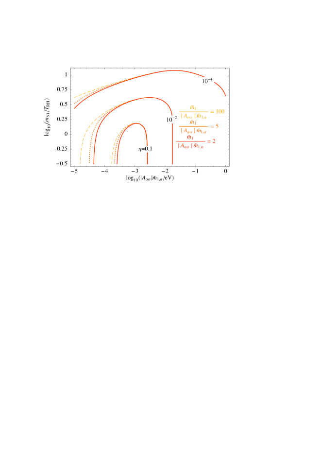
Figure 1: Contour lines for the flavour-dependent efficiency factor $\eta$ in the MSSM as a function of $|A_{\alpha\alpha}|\widetilde{m}_{1,\alpha}$ (no sum over $\alpha$) and $m_{N_{1}}/T_{\mathrm{RH}}$, for fixed values of $\widetilde{m}_{1}/(|A_{\alpha\alpha}|\widetilde{m}_{1,\alpha})$. We take $\widetilde{m}_{1}/(|A_{\alpha\alpha}|\widetilde{m}_{1,\alpha})=2,5$ and $100$, respectively corresponding to the solid, dotted and dashed contour lines.

3.1.3 Limitations and approximations of the computation

As this point, it is pertinent to summarise the approximations and assumptions leading to the calculation of the produced baryon asymmetry.

For the right-handed neutrino sector, we assume a hierarchical mass spectrum, which means that we do not take into account the possibility of resonant effects in leptogenesis [24]. Furthermore, we assume that only decays of $N_{1}$ (and $\widetilde{N}_{1}$) significantly contribute to the final asymmetry, thus neglecting contributions from the decays of $N_{2},N_{3}$ (and $\widetilde{N}_{2},\widetilde{N}_{3}$). This is justified when either the washout processes mediated by the lighter right-handed (s)neutrinos are sufficiently active for each flavour, and thus indeed destroy the asymmetries arising from the decays of the heavier right-handed (s)neutrinos, or when $T_{\mathrm{RH}}\ll m_{N_{2}},m_{N_{3}}$. It is important to notice that under certain conditions the heavier right-handed neutrinos can also play a role for leptogenesis [25], and should in principle be included.

We include reheating in the flavour-dependent MSSM Boltzmann equations in a simplified, but comparatively model-independent way, following Ref. [20]. We notice that in specific models of reheating after inflation, the prospects for leptogenesis can be different. In particular, we assume that the lightest right-handed (s)neutrinos are only produced by thermal scatterings during and after reheating. We also neglect the possibility of producing $N_{1}$ (and $\widetilde{N}_{1}$) from the decays of the scalar field $\phi$ responsible for reheating, or of producing $N_{1}$ (and $\widetilde{N}_{1}$) during preheating. It is further assumed that the maximally reached temperature during the reheating process, $T^{\mathrm{max}}$, as well as the mass of $\phi$, are much larger than $m_{N_{1}}$. Furthermore, we neglect the potential implications of supersymmetric flat directions for reheating and thermal leptogenesis, which are still under controversial discussion [28].

When solving the Boltzmann equations for flavour-dependent leptogenesis, we focus our attention on the case where, during the relevant temperatures for leptogenesis, the interactions mediated by each of the charged lepton Yukawa couplings are either fully in equilibrium, or out of equilibrium. In the MSSM, for values of $m_{N_{1}}$ around $(1+\tan^{2}\beta)\times 10^{9}$ GeV, the reactions induced by the muon Yukawa coupling are close to equilibrium and the quantum oscillations of the asymmetries may not have been dumped fast enough to be neglected. To take these effects into account, the Boltzmann equations may be generalised so to include quantum oscillations [10]. In this study, we chose $\tan\beta$ sufficiently large so that we can safely assume that the charged $\mu$ and $\tau$ Yukawa couplings are in thermal equilibrium, and that all flavours in the Boltzmann equations can be treated separately. Furthermore, we neglect the small off-diagonal elements of the matrix $A$, which appears in the washout terms of the Boltzmann equations for $\hat{Y}_{\Delta_{\alpha}}$ (c.f. Appendix A). We note that this approximation is crucial if one wants to introduce an efficiency factor $\eta$, which is a function of the ratio $m_{N_{1}}/T_{\mathrm{RH}}$, of the product $A_{\alpha\alpha}\,\widetilde{m}_{1,\alpha}$ (no sum over $\alpha$), and of the total washout parameter $\widetilde{m}_{1}$. We have numerically verified that in the regions of interest for this study, including the off-diagonal elements has only a small effect of increasing the produced BAU by about 20%.

Following Ref. [29], in our numerical computations we only include processes in the thermal bath mediated by neutrino and top Yukawa couplings. This means that we neglect $\Delta L=1$ scatterings involving gauge bosons [30, 20], thermal corrections [20] and possible effects from spectator processes [31], but that we do take into account corrections from renormalisation group (RG) running between the electroweak scale and $m_{N_{1}}$ [8, 32] (for which we use the software package REAP [33]). Regarding the pole mass of the top quark, we take the value $m_{t}^{\text{pole}}=174.2$ GeV [34]. We stress that the uncertainties in this value can have a strong influence on the RG evolution of the relevant parameters (namely the neutrino masses). Thus, the latter can provide a significant source of uncertainties in the BAU estimates. The renormalised value of the top Yukawa coupling (at energies $m_{N_{1}}$), also directly affects the strength of the $\Delta L=1$ scatterings. Furthermore, let us notice that we also neglect $\Delta L=2$ scatterings, which is a good approximation as long as $|A_{\alpha\alpha}|\widetilde{m}_{1,\alpha}/m^{*}\gg 10\times(m_{N_{1}}/10^{14}\>\mbox{GeV})$ [12].

Finally, our estimates of the produced BAU are based on a set of coupled Boltzmann equations, which only provide a classical approximation to the Kadanoff-Baym equations. Quantum effects for thermalization have been ignored in our analysis [35]. Other approximations have led to the present simplified form of the Boltzmann equations: for instance, it is usually assumed that elastic scattering rates are fast and that the phase space densities for both fermions and scalars can be approximated as $f(E_{i},T)=(n_{i}/n^{\mathrm{eq}}_{i})e^{-E_{i}/T}$, where $n_{i}^{\mathrm{eq}}=\tfrac{g_{i}}{2\pi}Tm_{i}^{2}K_{2}(m_{i}/T)$, with $g_{i}$ being the number of degrees of freedom. Accordingly, we also use the equilibrium number densities in this so-called Boltzmann approximation.

All the above mentioned approximations (as well as others we have not explicitly discussed) will ultimately translate in potentially relevant theoretical uncertainties when estimating the value of the BAU. Thus, it is important to bare in mind that one may be either over- or under-estimating $n_{\text{B}}/n_{\gamma}$, so that caution should be exerted when deciding upon the BAU viability of a given SUSY seesaw scenario.

3.2 Constraints on the reheat temperature and the gravitino problem

The predictions for the baryon asymmetry arising from a given seesaw scenario can be severely compromised due to constraints on $T_{\mathrm{RH}}$. One important example of such constraints emerges in locally supersymmetric theories, and stems from the decays of thermally produced gravitinos [36, 37]. In this class of SUSY models, and assuming a low-energy MSSM with R-parity conservation, either the gravitino is the lightest supersymmetric particle (LSP) and is thus stable, or else it will ultimately decay into the LSP. Two generic problems arise from these decays, and are the following.

Firstly, gravitinos can decay late, after the Big Bang nucleosynthesis (BBN) epoch, and potentially spoil the success of BBN [36, 38]. This leads to upper bounds on the reheat temperature which depend on the specific supersymmetric model as well as on the mass of the gravitino [37]. For gravitino masses in the TeV region, the gravitino BBN problem practically precludes the possibility of thermal leptogenesis. However, with a heavy gravitino (roughly above $100$ TeV), the BBN problems can be nearly avoided. If one considers the gravitino mass as a free parameter, one can safely avoid the latter constraints for any given reheat temperature.

Secondly, the decay of a gravitino produces one LSP, which has an impact on the relic density of the latter. The number of thermally produced gravitinos increases with the reheat temperature, and we can estimate the contribution to the dark matter (DM) relic density arising from non-thermally produced LSPs via gravitino decay (for heavy gravitinos) as [38, 37]

$$\Omega^{\mathrm{non-th}}_{\mathrm{LSP}}\,h^{2}\approx 0.054\left(\frac{m_{\mathrm{LSP}}}{100\,\text{GeV}}\right)\left(\frac{T_{\mathrm{RH}}}{10^{10}\,\text{GeV}}\right),$$ (18)

which depends on the LSP mass, $m_{\mathrm{LSP}}$, as well as on $T_{\mathrm{RH}}$. Taking the relic density bound $\Omega^{\mathrm{non-th}}_{\mathrm{LSP}}h^{2}\leq\Omega_{\mathrm{DM}}h^{2}\lesssim 0.13$ from the Wilkinson Microwave Anisotropy Probe (WMAP) [1], we are led to an upper bound on the reheat temperature of

$$T_{\mathrm{RH}}\,\lesssim\,2.4\times 10^{10}\,\text{GeV}\,\left(\frac{100\>\text{GeV}}{m_{\mathrm{LSP}}}\right).$$ (19)

For masses of the LSP (assuming this to be the lightest neutralino) in the range 100 GeV$\,-\,150$ GeV we obtain an estimated upper bound on the reheat temperature of approximately $T_{\mathrm{RH}}\lesssim 2\,\times\,10^{10}\,\text{GeV}$. Naturally, heavier LSP masses lead to more severe bounds on $T_{\mathrm{RH}}$.

There are other frameworks where, although still viable, thermal leptogenesis is significantly constrained by bounds on $T_{\mathrm{RH}}$. This can occur for scenarios with stable gravitinos, i.e. where gravitinos are the LSP. In many cases the bounds on the reheat temperature strongly depend on the model under consideration, for instance on the properties of the next-to-lightest supersymmetric particle (NLSP). For example, recent studies of models with gravitino LSP [39] have found the following bounds for the Constrained Minimal Supersymmetric Standard Model (CMSSM),

$$T_{\mathrm{RH}}\lesssim 4\,\times\,10^{9}\,\text{GeV}\,,$$ (20)

while a scenario with gaugino-mediated supersymmetry breaking and sneutrino NLSP (stau NLSP) implies [40]

$$T_{\mathrm{RH}}\lesssim 7\,\times\,10^{9}\,\text{GeV}\;\;(T_{\mathrm{RH}}\lesssim 3\,\times\,10^{9}\,\text{GeV})\;.$$ (21)

In the subsequent numerical analysis, and as examples, we will take into account the following bounds, $T_{\mathrm{RH}}\leq 2\,\times\,10^{10}\,\text{GeV}$ and $T_{\mathrm{RH}}\leq 5\,\times\,10^{9}\,\text{GeV}$, respectively representative of a mildly and a strongly constrained case for thermal leptogenesis.

4 Constraints on the seesaw parameters

After having gone through the most relevant aspects of the computation of the BAU, let us now proceed to discuss the constraints on the several seesaw parameters which arise from assuming that the baryon asymmetry is generated by flavour-dependent thermal leptogenesis.

The parameters of the $U_{\text{MNS}}$ matrix, as well as the two mass squared differences, are presently constrained by neutrino oscillation experiments. From them we know that $s_{23}\approx c_{23}\approx\sqrt{1/2}$, $s_{12}\approx\sqrt{1/3}$ (and $c_{12}\approx\sqrt{2/3}$), while $\theta_{13}$ is only bounded from above, $\theta_{13}\lesssim 11.5^{\circ}$ (at $3\sigma$ confidence level) [41]. Regarding the Dirac and Majorana phases ($\delta$, $\varphi_{1}$ and $\varphi_{2}$), no experimental data is yet available. For the case of hierarchical neutrinos, we have that $m_{\nu_{2}}\approx\sqrt{\Delta m^{2}_{\text{sol}}}\approx 0.01$ eV and $m_{\nu_{3}}\approx\sqrt{\Delta m^{2}_{\text{atm}}}\approx 0.05$ eV. On the other hand, parameters like the heavy neutrino masses $m_{N_{i}}$, and the mixing angles involving the heavy Majorana neutrinos (i.e. the complex $R$-matrix angles $\theta_{i}$), are experimentally unreachable.

The main focus of this work is to address the constraints on mixing angles and CP violating phases of both the light and heavy neutrino sectors. However, and especially when reheating effects are taken into account, interesting bounds for the heavy and light neutrino masses can also be derived. We begin our discussion by briefly re-analysing the latter constraints for the case of the MSSM, considering flavour-dependent effects.

4.1 Heavy and light neutrino masses

Let us start with general considerations regarding bounds on the light and heavy neutrino masses from thermal leptogenesis in the MSSM, when flavour effects are taken into account. From Eqs. (14, 17), it is clear that within our framework (and approximations), the masses $m_{N_{2}}$ and $m_{N_{3}}$ are not constrained by thermal leptogenesis.

In flavour-dependent leptogenesis, the decay asymmetries are constrained by [12]

$$\varepsilon_{1,\alpha}\,\leq\,\frac{3\,m_{N_{1}}}{8\pi\,v_{2}^{2}}\,m_{\nu_{3}}\,\left(\frac{\widetilde{m}_{1,\alpha}}{\widetilde{m}_{1}}\right)^{1/2}\,\equiv\,\varepsilon^{\mathrm{max}}_{1}\,\left(\frac{\widetilde{m}_{1,\alpha}}{\widetilde{m}_{1}}\right)^{1/2}.$$ (22)

In the above equation, and for hierarchical light neutrino masses, $\varepsilon^{\mathrm{max}}_{1}=3\,m_{N_{1}}\,m_{\nu_{3}}/(8\pi\,v_{2}^{2})$ is the maximally possible value, both in the flavour-independent approximation and in the flavour-dependent treatment. Regarding washout, in the type-I seesaw, the flavour-independent washout parameter satisfies [42]

$$\widetilde{m}_{1}\,\geq\,m_{\nu_{1}}\;,$$ (23)

whereas the flavour-dependent washout parameters $\widetilde{m}_{1,\alpha}$ are generically not constrained. In the flavour-independent approximation, Eq. (23) leads to a dramatically more restrictive bound on $\varepsilon_{1}=\sum_{\alpha}\varepsilon_{1,\alpha}$ [21], and finally even to a bound on the neutrino mass scale [42]. We also note that for quasi-degenerate light neutrino masses, an optimal washout parameter $\widetilde{m}_{1,\alpha}\approx m^{*}$ is possible, but it however implies that the decay asymmetries are suppressed by at least a factor $\sqrt{m^{*}/m_{\nu_{1}}}$ when compared to the optimal value $\varepsilon^{\mathrm{max}}_{1}$ (c.f. Eq. (22)). Concerning the decay asymmetries, we will see that the suppression factor $\sqrt{\widetilde{m}_{1,\alpha}/\widetilde{m}_{1}}$ has further interesting implications also for the case of hierarchical neutrino masses.

Using the upper bound on the decay asymmetry of Eq. (22) for the case of hierarchical light neutrinos, and assuming an optimal efficiency, it is possible to estimate the baryon asymmetry. Even without reheating, the comparison of the estimated value with the observed BAU by WMAP [1],

$$n_{\mathrm{B}}/n_{\gamma}\,\approx\,(6.10\,\pm\,0.21)\,\times\,10^{-10}\,,\quad\text{or}\quad Y_{B}\,\approx\,(0.87\,\pm\,0.03)\,\times\,10^{-10}\,,$$ (24)

allows to obtain a lower bound on the mass $m_{N_{1}}$ of the lightest right-handed neutrino [21].

Clearly, the maximal BAU that can be generated depends on both $m_{N_{1}}$ and $T_{\mathrm{RH}}$. The combined constraints on these quantities are shown in Fig. 2. Leading to the latter, we have considered a normal hierarchical spectrum of light neutrinos. We have also assumed a maximal decay asymmetry as in Eq. (22) and an optimal efficiency for a given $m_{N_{1}}/T_{\mathrm{RH}}$. From Fig. 2, let us finally point out that in order to obtain BAU compatible with the WMAP range (represented in dark blue), the minimal values for the reheat temperature and for $m_{N_{1}}$ are $T^{\mathrm{min}}_{\mathrm{RH}}\approx 1.9\times 10^{9}$ GeV and $m^{\mathrm{min}}_{N_{1}}\approx 1.5\times 10^{9}$ GeV. Moreover, in the presence of an upper bound on the reheat temperature, there is also an upper bound on $m_{N_{1}}$, stemming from the dramatic loss of efficiency occurring when $m_{N_{1}}\gg T_{\mathrm{RH}}$, as it was shown in Fig. 1. For instance, $T_{\text{RH}}\lesssim 2\times 10^{10}$ GeV imposes $m^{\text{max}}_{N_{1}}\approx 1.4\times 10^{11}$ GeV, while $T_{\text{RH}}\lesssim 5\times 10^{9}$ GeV yields $m^{\text{max}}_{N_{1}}\approx 1.9\times 10^{10}$ GeV, leading to viability windows for the mass of the lightest right-handed neutrino.

Figure 2: Isosurfaces corresponding to the maximally possible BAU as function of $m_{N_{1}}$ and $T_{\mathrm{RH}}$. From small to large $m_{N_{1}}-T_{\mathrm{RH}}$ regions, the associated BAU ranges are: $n_{\text{B}}/n_{\gamma}\in[10^{-10},\,3\times 10^{-10}]$, $n_{\text{B}}/n_{\gamma}\in[3\times 10^{-10},\,5.9\times 10^{-10}]$, $n_{\text{B}}/n_{\gamma}\in[5.9\times 10^{-10},\,6.3\times 10^{-10}]$, $n_{\text{B}}/n_{\gamma}\in[6.3\times 10^{-10},\,10^{-9}]$ and $n_{\text{B}}/n_{\gamma}\gtrsim 10^{-9}$. The corresponding colour code is grey, green, dark blue (WMAP), light blue and red, respectively.

In the following analysis, whenever we present numerical examples regarding constraints on the seesaw parameters, we will vary $m_{N_{1}}$, and select the value for which the produced baryon asymmetry is maximal. Typically, this corresponds to $m_{N_{1}}$ around (or slightly above) $T_{\mathrm{RH}}$, as illustrated in Fig. 3. In order to reduce the BAU associated with a given choice of parameters, one can simply vary $m_{N_{1}}$. Lowering $m_{N_{1}}$ such that $m_{N_{1}}\ll m^{*}$ leads to a regime where $n_{\text{B}}/n_{\gamma}$ decreases with decreasing $m_{N_{1}}$. On the other hand, it is also possible to increase $m_{N_{1}}$, taking values $m_{N_{1}}\gg T_{\text{RH}}$, since then the strong washout leads to an important reduction in the BAU.

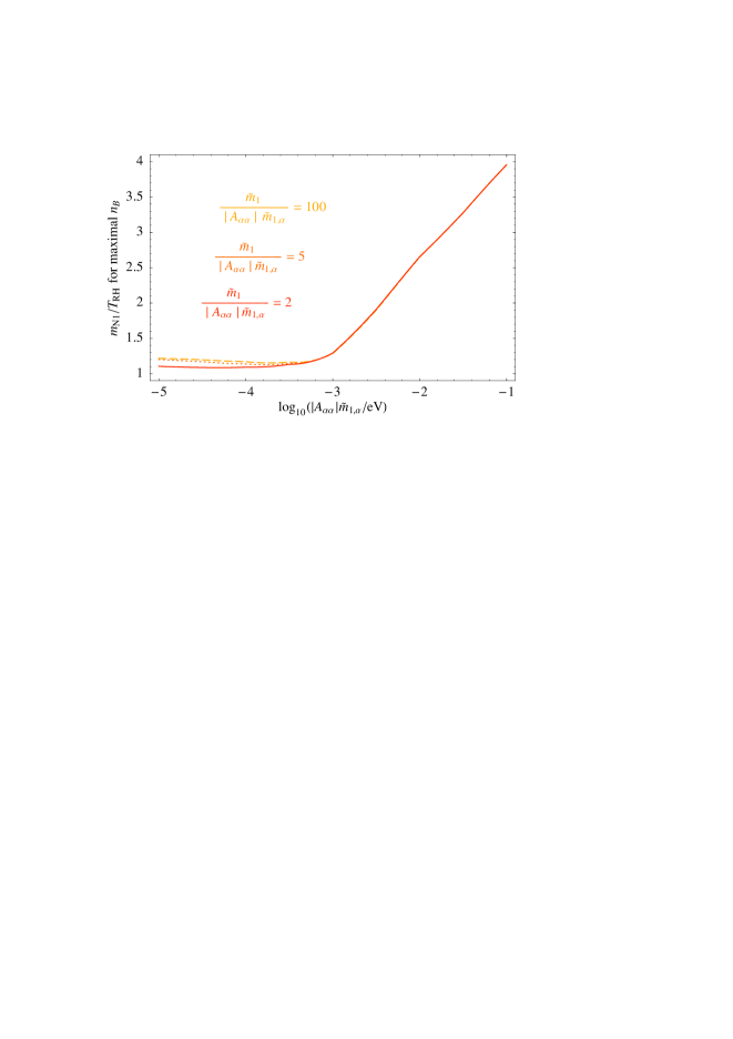
Figure 3: Value of the ratio $m_{N_{1}}/T_{\mathrm{RH}}$ which yields the maximally possible baryon asymmetry, as a function of $|A_{\alpha\alpha}|\widetilde{m}_{1,\alpha}$. Solid, dotted, and dashed lines correspond to $\widetilde{m}_{1}/(|A_{\alpha\alpha}|\,\widetilde{m}_{1,\alpha})=2,5$ and $100$, respectively.

Finally, and before concluding this discussion, let us comment on the bounds for the masses of the light neutrinos. At present, the absolute neutrino mass scale $m_{\nu_{1}}$ (for normal mass ordering) is only experimentally constrained by Tritium $\beta$-decay, $0\nu\beta\beta$-decay and cosmology, to be roughly below $0.5$ eV [45]. In general, flavour-dependent leptogenesis will not provide any additional constraints on $m_{\nu_{1}}$. As mentioned before, in the present study we focus on hierarchical light neutrinos. In this case, it is nevertheless interesting to point out that with a bound $T_{\mathrm{RH}}\leq 5\times 10^{9}$ GeV or $T_{\mathrm{RH}}\leq 2\times 10^{10}$ GeV, we have numerically verified that increasing the neutrino mass scale towards a quasi-degenerate light neutrino mass spectrum leads to a reduction of the BAU-allowed regions of the parameter space. This is essentially due to two reasons. Firstly, although there is no bound on $\widetilde{m}_{1,\alpha}$, its typical values are of the order of $m_{\nu_{1}},m_{\nu_{2}}$ and $m_{\nu_{3}}$. Therefore, only for strongly hierarchical light neutrino masses can $m_{\nu_{1}}$ set the right scale for an optimal washout parameter. Secondly, slightly increasing $m_{\nu_{1}}$ towards a quasi-degenerate spectrum does not significantly enhance $\varepsilon_{1}^{\mathrm{max}}$, but does reduce each of the decay asymmetries due to a factor of $\sqrt{\widetilde{m}_{1,\alpha}/\widetilde{m}_{1}}\approx\sqrt{m^{*}/\widetilde{m}_{1}}<\sqrt{m^{*}/m_{\nu_{1}}}$, enforcing optimal washout $\widetilde{m}_{1,\alpha}\approx m^{*}$ (using Eq. (23)). This is illustrated in Fig. 4, where we display the bound on the decay asymmetry $\varepsilon_{1,\alpha}$, normalised to the maximal decay asymmetry $\varepsilon^{\mathrm{max,}0}=\frac{3\,m_{N_{1}}}{8\pi\,v_{2}^{2}}\,\sqrt{\Delta m^{2}_{\text{atm}}}\,$ for a (normal) hierarchical mass spectrum of light neutrinos. The washout parameter $\widetilde{m}_{1,\alpha}$ has been fixed to $m^{*}=\sin^{2}\beta\times 1.58\times 10^{-3}$ (close to its optimal value).

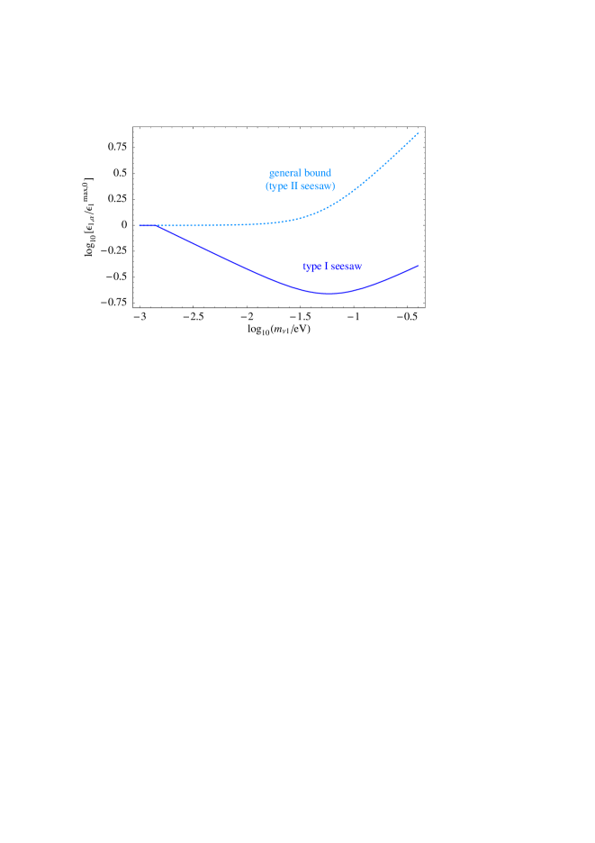
Figure 4: Bound on the decay asymmetry $\varepsilon_{1,\alpha}$ as a function of $m_{\nu_{1}}$. The washout parameter $|A_{\alpha\alpha}|\widetilde{m}_{1,\alpha}$ is fixed to $m^{*}=\sin^{2}\beta\times 1.58\times 10^{-3}$ (close to optimal), and the asymmetry is normalised to its maximal value $\varepsilon^{\mathrm{max,}0}$, obtained for a (normal) hierarchical mass spectrum of light neutrinos with $m_{\nu_{1}}=0$. The bound of the decay asymmetry in the type-I seesaw (solid line) decreases with increasing neutrino mass scale and remains below the bound for hierarchical masses for the depicted values of $m_{\nu_{1}}<0.4$ eV. For comparison, the general bound, which can be saturated in the type-II seesaw scenario, is also displayed (dotted line). The latter increases with increasing neutrino mass scale. We have used $\tan\beta=30$ and $m_{N_{1}}=10^{10}$ GeV.

4.2 Mixing angles and CP phases

Here we will discuss how the constraints arising from the reheat temperature can affect the washout and efficiency factors, and in turn favour/disfavour choices for the mixing angles and CP violating phases. We also analyse the impact of the latter constraints regarding the flavour-dependent CP asymmetries, and investigate some illustrative limits regarding the $R$-matrix angles, $\theta_{i}$.

4.2.1 Favoured parameter regions with optimal washout

With strong constraints on the reheat temperature like $T_{\mathrm{RH}}\leq 5\times 10^{9}$ GeV or $T_{\mathrm{RH}}\leq 2\times 10^{10}$ GeV (motivated by Eqs. (19-21)), and a lower bound on $m_{N_{1}}$ of about $10^{9}$ GeV, only a rather small window of $m_{N_{1}}$ values remains allowed (c.f. Fig. 2). This means that in order to produce enough baryon asymmetry, at least one of the efficiency factors $\eta_{\alpha}=\eta(A_{\alpha\alpha}\widetilde{m}_{1,\alpha},\widetilde{m}_{1},T_{\mathrm{RH}}/m_{N_{1}})$ should be close to optimal (i.e., $\widetilde{m}_{1,\alpha}$ must not differ much from $m^{*}$) and, in addition, the corresponding decay asymmetries should approach $\varepsilon_{1}^{\mathrm{max}}$.

An optimal efficiency $\eta$ can be achieved for $\widetilde{m}_{1,\alpha}\approx m^{*}=\sin^{2}\beta\times 1.58\times 10^{-3}$ eV. Note that $m^{*}$ is much smaller than $m_{\nu_{3}}$ and, even though $m_{\nu_{2}}<m_{\nu_{3}}$, $m^{*}$ is still significantly smaller than $m_{\nu_{2}}$. For hierarchical light neutrino masses, apart from having $m_{\nu_{1}}\ll m_{\nu_{2}}<m_{\nu_{3}}$, $m_{\nu_{1}}$ is unconstrained and can vary in a large range. For instance, it is possible to choose $m_{\nu_{1}}$ close to $m^{*}$, such that $\widetilde{m}_{1,\alpha}\approx m_{\nu_{1}}$ would ensure an optimal value for the washout parameter. In the following numerical analysis, we will set $m_{\nu_{1}}=10^{-3}\>\mbox{eV}\approx m^{*}$ as an illustrative example.

To begin the analysis, let us start by writing the washout parameters explicitly in terms of the seesaw parameters, using the $R$-matrix parameterisation. One has

$$\widetilde{m}_{1,e} = \big{|}e^{\frac{i}{2}\varphi_{1}}\,c_{2}\,c_{3}\,c_{12}\,c_{13}\,\sqrt{m_{\nu_{1}}}+s_{3}(e^{i\delta}\,s_{1}\,s_{13}\,\sqrt{m_{\nu_{3}}}-e^{\frac{i}{2}\varphi_{2}}\,c_{1}\,s_{12}\,c_{13}\,\sqrt{m_{\nu_{2}}})$$ (25)

$$+s_{2}c_{3}(-e^{i\delta}\,c_{1}\,s_{13}\,\sqrt{m_{\nu_{3}}}-e^{\frac{i}{2}\varphi_{2}}\,s_{1}\,s_{12}\,c_{13}\,\sqrt{m_{\nu_{2}}})\big{|}^{2},$$

$$\widetilde{m}_{1,\mu} = \big{|}-e^{\frac{i}{2}\varphi_{1}}\,c_{2}\,c_{3}\,s_{12}\,c_{23}\,\sqrt{m_{\nu_{1}}}+s_{3}(s_{1}\,s_{23}\,\sqrt{m_{\nu_{3}}}-e^{\frac{i}{2}\varphi_{2}}\,c_{1}\,c_{12}\,c_{23}\,\sqrt{m_{\nu_{2}}})$$ (26)

$$+s_{2}c_{3}(-c_{1}\,s_{23}\,\sqrt{m_{\nu_{3}}}-e^{\frac{i}{2}\varphi_{2}}\,s_{1}\,c_{12}\,c_{23}\,\sqrt{m_{\nu_{2}}})+{\cal O}(\theta_{13})\big{|}^{2},$$

$$\widetilde{m}_{1,\tau} = \big{|}e^{\frac{i}{2}\varphi_{1}}\,c_{2}\,c_{3}\,s_{12}\,s_{23}\,\sqrt{m_{\nu_{1}}}+s_{3}(s_{1}\,c_{23}\,\sqrt{m_{\nu_{3}}}+e^{\frac{i}{2}\varphi_{2}}\,c_{1}\,c_{12}\,s_{23}\,\sqrt{m_{\nu_{2}}})$$ (27)

$$s_{2}c_{3}(-c_{1}\,c_{23}\,\sqrt{m_{\nu_{3}}}+e^{\frac{i}{2}\varphi_{2}}\,s_{1}\,c_{12}\,s_{23}\,\sqrt{m_{\nu_{2}}})+{\cal O}(\theta_{13})\big{|}^{2}.$$

For $\widetilde{m}_{1,\mu},\widetilde{m}_{1,\tau}$, only the zeroth order terms in an expansion in $\theta_{13}$ are shown. We note that, when compared to $\theta_{2}$ and $\theta_{3}$, $\theta_{1}$ only plays a minor role for leptogenesis. This can be clarified by considering the second and third terms on the right side of the equations, which contain the two potentially large contributions associated with $\sqrt{m_{\nu_{2}}}$ and $\sqrt{m_{\nu_{3}}}$. As can be seen, a real $\theta_{1}$ mainly rotates terms proportional to $\sqrt{m_{\nu_{2}}}$ into terms proportional to $\sqrt{m_{\nu_{3}}}$, and thus it is not introducing any new features. For instance, with $\theta_{1}=\pi/2$, the roles of $\theta_{2}$ and $\theta_{3}$ are simply interchanged: a $\theta_{2}$ rotation now generates contributions to $\widetilde{m}_{1,\alpha}$ of ${\cal O}(m_{\nu_{2}})$ and a $\theta_{3}$ rotation induces contributions to $\widetilde{m}_{1,\alpha}$ of ${\cal O}(m_{\nu_{3}})$. Large imaginary parts of $\theta_{1}$ typically lead to $\widetilde{m}_{1,\alpha}>m_{\nu_{1}}\approx m^{*}$, and thus are not useful in achieving optimal efficiencies. Although it is straightforward to generalise the discussion to include arbitrary $\theta_{1}$, we will simplify the analysis by setting $\theta_{1}=0$ in what follows. In the limit of $\theta_{1}=0$, we find

$$\widetilde{m}_{1,e} \approx \big{|}e^{\frac{i}{2}\varphi_{1}}\,c_{2}\,c_{3}\,c_{13}\,c_{12}\,\sqrt{m_{\nu_{1}}}-e^{\frac{i}{2}\varphi_{2}}\,s_{3}\,s_{12}\,c_{13}\,\sqrt{m_{\nu_{2}}}-e^{i\delta}\,s_{2}\,c_{3}\,s_{13}\,\sqrt{m_{\nu_{3}}}\big{|}^{2},$$ (28)

$$\widetilde{m}_{1,\mu} \approx \big{|}-e^{\frac{i}{2}\varphi_{1}}\,c_{2}\,c_{3}\,s_{12}\,c_{23}\,\sqrt{m_{\nu_{1}}}-e^{\frac{i}{2}\varphi_{2}}\,s_{3}\,c_{12}\,c_{23}\,\sqrt{m_{\nu_{2}}}-s_{2}\,c_{3}\,s_{23}\,\sqrt{m_{\nu_{3}}}\big{|}^{2},$$ (29)

$$\widetilde{m}_{1,\tau} \approx \big{|}e^{\frac{i}{2}\varphi_{1}}\,c_{2}\,c_{3}\,s_{12}\,s_{23}\,\sqrt{m_{\nu_{1}}}+e^{\frac{i}{2}\varphi_{2}}\,s_{3}\,c_{12}\,s_{23}\,\sqrt{m_{\nu_{2}}}-s_{2}\,c_{3}\,c_{23}\,\sqrt{m_{\nu_{3}}}\big{|}^{2},$$ (30)

where, as in Eqs. (26, 27), only the zeroth order terms in an expansion in $\theta_{13}$ are shown for $\widetilde{m}_{1,\mu},\widetilde{m}_{1,\tau}$. In general, for an optimal efficiency, it is crucial to avoid contributions to $\widetilde{m}_{1,\alpha}$ of order ${\cal O}(m_{\nu_{2}})$ or ${\cal O}(m_{\nu_{3}})$. In the flavour-independent approximation, achieving an optimal washout (given by the sum $\widetilde{m}_{1}=\sum_{\alpha}\widetilde{m}_{1,\alpha}$) necessarily required that both $|s_{2}|$ and $|s_{3}|$ were small [19]. As can be seen from Eqs. (28-30), when flavour effects are included, washout considerations still favour parameter regions with small $|s_{2}|$ and $|s_{3}|$. Nevertheless, in the flavour-dependent treatment, the individual washout parameters $\widetilde{m}_{1,\alpha}$ are typically smaller than their sum, $\widetilde{m}_{1}$, and can significantly differ from each other. It is therefore pertinent to re-investigate whether other regions of parameter space may also allow for optimal washout.

Let us first consider the contribution to $\widetilde{m}_{1,\tau}$ (or similarly to $\widetilde{m}_{1,\mu}$) proportional to $m_{\nu_{2}}$, due to non-zero values of $\theta_{3}$. From Eq. (30) we find that this is given by $c_{12}^{2}\,s_{23}^{2}\,s^{2}_{3}\,m_{\nu_{2}}\,\approx\,\tfrac{1}{3}\,s^{2}_{3}\,m_{\nu_{2}}$. In addition, the quantity which enters the efficiency factor is the product $A_{\tau\tau}\widetilde{m}_{1,\tau}$, with $A_{\tau\tau}\approx-0.6$. Combining these two effects reduces the $\theta_{3}$-induced washout by a factor of about $1/5$, and even for $s_{3}\approx{\cal O}(1)$ optimal washout $|A_{\alpha\alpha}|\widetilde{m}_{1,\alpha}\approx m^{*}$ is still possible to obtain. On the other hand, the contribution to $\widetilde{m}_{1,\tau}$ (or similarly to $\widetilde{m}_{1,\mu}$) proportional to $m_{\nu_{3}}$ due to non-zero $\theta_{2}$ is given by $c_{23}^{2}\,s^{2}_{2}\,c^{2}_{3}\,m_{\nu_{3}}\,\approx\,\tfrac{1}{2}\,s^{2}_{3}\,c^{2}_{3}\,m_{\nu_{3}}$. Again, the quantity which enters the efficiency factor is the product $|A_{\tau\tau}|\widetilde{m}_{1,\tau}$. Although combining these two effects reduces the $\theta_{2}$-induced washout by a factor of about $0.3$, optimal washout cannot be achieved for large $|s_{2}|$, if $\theta_{3}$ is small. The only exception occurs for small $|c_{3}|$, which can suppress the large contribution of ${\cal O}(m_{\nu_{3}})$ to $\widetilde{m}_{1,\tau},\widetilde{m}_{1,\mu}$ and still allow for large $|s_{2}|$. However, as we will see in the next subsection, the decay asymmetries $\varepsilon_{1,\alpha}$ are somewhat suppressed in this case.

Another difference between the flavour-independent approximation and the correct flavour-dependent treatment becomes apparent when we consider $\widetilde{m}_{1,e}$. In contrast to $\widetilde{m}_{1,\tau}$ and $\widetilde{m}_{1,\mu}$, large values of $s_{2}$ only induce a washout parameter $\widetilde{m}_{1,e}$ of $s^{2}_{13}\times{\cal O}(m_{\nu_{3}})$. In other words, we can be in the optimal washout regime $\widetilde{m}_{1,e}\approx m^{*}$ also for larger values of $s_{2}$, depending on the size of $\theta_{13}$. Nevertheless, in this case the decay asymmetry $\varepsilon_{1,e}$ is also suppressed when compared to the optimal regime.

Let us point out that another possible way to obtain optimal $\widetilde{m}_{1,\mu}$ and $\widetilde{m}_{1,\tau}$ of order $m^{*}$ would be to align $s_{2}$ and $s_{3}$ such that their contributions to one of the washout parameters (respectively proportional to $m_{\nu_{3}}$ and $m_{\nu_{2}}$) would nearly cancel each other. In this case one could obtain, for example, $\widetilde{m}_{1,\mu}\approx m^{*}$. However, one can verify that the third washout parameter $\widetilde{m}_{1,\tau}$ (and thus $\widetilde{m}_{1}$) would still be ${\cal O}(m_{\nu_{3}})$ or ${\cal O}(m_{\nu_{2}})$, which would imply a suppression of $\varepsilon_{1,\mu}$ by a factor $m^{*}/\widetilde{m}_{1}$, in comparison to $\varepsilon_{1}^{\mathrm{max}}$ (c.f. Eq. (22)).

4.2.2 Flavour-Dependent Decay Asymmetries

From the analysis of the flavour-dependent washout parameters $\widetilde{m}_{1,\alpha}$, it has become apparent that there are several regions of the seesaw parameter space with appealing prospects for leptogenesis. They can be summarised as follows. Generically favoured is the region of small $|s_{2}|$ and $|s_{3}|$, where the washout parameters $\widetilde{m}_{1,\alpha}$ are ${\cal O}(m_{\nu_{1}})$, and receive only small contributions proportional to $m_{\nu_{2}}$ and $m_{\nu_{3}}$. In the flavour-independent approximation, this was the only region favoured by washout [19]. In contrast, in flavour-dependent leptogenesis, washout (in all flavours) remains optimal also for larger values of $|s_{3}|\lesssim 1$. With small $|c_{3}|$ (implying large $|s_{3}|$ which is no longer disfavoured), large $|s_{2}|$ becomes compatible with optimal washout, and a whole new region, washout-favoured, has emerged. An additional interesting effect is that washout in the $e$-flavour, governed by $\widetilde{m}_{1,e}$, can also be optimal for large $|s_{2}|$, due to the smallness of $\theta_{13}$.

In addition to an optimal $\widetilde{m}_{1,\alpha}$, and given the tight constraints on the reheat temperature, it is also desirable to have decay asymmetries close to the optimal value $\varepsilon_{1}^{\mathrm{max}}$. Let us now address the latter issue more thoroughly. First, we note that for $R=\mathbbm{1}$, and more generally, for $\theta_{i}=0,\tfrac{\pi}{2}$ (mod $\pi$), the decay asymmetries exactly vanish. A deviation from the latter values of the form $\theta_{2}=\theta_{3}=0$ but $\theta_{1}\not=0$, also leads to zero values. To clarify the analysis, let us explicitly write the decay asymmetries in terms of the seesaw parameters. For simplicity, and as illustrative examples, we first consider the dependence on $\theta_{2}$, with $\theta_{3}=\theta_{1}=0$, and then study the $\theta_{3}$-dependence, setting $\theta_{2}=\theta_{1}=0$. To discuss the parameter regions with optimal washout where $\theta_{2}$ and $\theta_{3}$ are both large, we then turn to the decay asymmetries with nonzero $\theta_{2}$ and $\theta_{3}$. For simplicity, in the latter case we will again present the formulae with $\theta_{1}=0$. The discussion can be easily generalised to arbitrary $\theta_{i}$ values, using the general expressions for the decay asymmetries as given in Eqs. (12, 14). We will also illustrate the effects of nonzero $\theta_{1}$ via numerical examples in Section 4.3.

For $\theta_{3}=\theta_{1}=0$, one obtains

$$\varepsilon_{1,e}\! \approx \!-\frac{3\,m_{N_{1}}}{8\,\pi\,v_{2}^{2}\,(|c_{2}|^{2}\,{m_{\nu_{1}}}+|s_{2}|^{2}\,{m_{\nu_{3}}})}\,\mathrm{Im}\left[\,{s^{2}_{13}}\,{s^{2}_{2}}\,m_{\nu_{3}}^{2}\,\right.$$ (31)

$$\left.-\,e^{\frac{\mathrm{i}}{2}({{\varphi}_{1}}-2\,\delta)}\,{s_{13}}\,{c_{13}}\,{c_{12}}\,{s_{2}}\,{c_{2}}\,{\sqrt{m_{\nu_{1}}}}\,m_{\nu_{3}}^{\frac{3}{2}}+\dots\right]\,,$$

$$\varepsilon_{1,\mu}\! \approx \!-\frac{3\,m_{N_{1}}}{8\,\pi\,v_{2}^{2}\,(|c_{2}|^{2}\,{m_{\nu_{1}}}+|s_{2}|^{2}\,{m_{\nu_{3}}})}\,\mathrm{Im}\left[\,{s^{2}_{23}}\,{s^{2}_{2}}\,{c^{2}_{13}}\,m_{\nu_{3}}^{2}\,\right.$$ (32)

$$\left.+\,e^{\frac{\mathrm{i}}{2}{{\varphi}_{1}}}{c_{13}}\,\,{s_{12}}\,{s_{23}}\,{c_{23}}\,{s_{2}}\,{c_{2}}\,{\sqrt{m_{\nu_{1}}}}\,m_{\nu_{3}}^{\frac{3}{2}}\right.$$

$$\left.+\,e^{\frac{\mathrm{i}}{2}({{\varphi}_{1}}-2\delta)}\,{s_{13}}\,{c_{13}}\,{c_{12}}\,{s^{2}_{23}}\,{s_{2}}\,{c_{2}}\,{\sqrt{m_{\nu_{1}}}}\,m_{\nu_{3}}^{\frac{3}{2}}+\dots\right]\,,$$

$$\varepsilon_{1,\tau}\! \approx \!-\frac{3\,m_{N_{1}}}{8\,\pi\,v_{2}^{2}\,(|c_{2}|^{2}\,{m_{\nu_{1}}}+|s_{2}|^{2}\,{m_{\nu_{3}}})}\,\mathrm{Im}\left[\,{c^{2}_{23}}\,{s^{2}_{2}}\,{c^{2}_{13}}\,m_{\nu_{3}}^{2}\,\right.$$ (33)

$$\left.-\,e^{\frac{\mathrm{i}}{2}{{\varphi}_{1}}}\,{c_{13}}\,{s_{12}}\,{s_{23}}\,{c_{23}}\,{s_{2}}\,{c_{2}}\,{\sqrt{m_{\nu_{1}}}}\,m_{\nu_{3}}^{\frac{3}{2}}\right.$$

$$\left.+\,e^{\frac{\mathrm{i}}{2}({{\varphi}_{1}}-2\delta)}\,{s_{13}}\,{c_{13}}\,{c_{12}}\,{c^{2}_{23}}\,{s_{2}}\,{c_{2}}\,{\sqrt{m_{\nu_{1}}}}\,m_{\nu_{3}}^{\frac{3}{2}}+\dots\right]\,,$$

where the dots indicate terms ${\cal O}(m_{\nu_{1}}^{\frac{3}{2}}\,\sqrt{m_{\nu_{3}}})$ and ${\cal O}(m_{\nu_{1}}^{2})$, which are sub-leading for hierarchical light neutrinos. Eqs. (32, 33) show that, provided that $\theta_{2}$ has an imaginary part, the $\theta_{2}$-induced decay asymmetries $\varepsilon_{1,\mu}$ and $\varepsilon_{1,\tau}$ can be close to the optimal value $\varepsilon_{1}^{\mathrm{max}}$ defined in Eq. (22). Regarding the sub-leading terms in Eqs. (32, 33), decay asymmetries can also emerge if the Majorana CP phase $\varphi_{1}$ is nonzero, albeit suppressed by a factor ${\cal O}(\sqrt{m_{\nu_{1}}/m_{\nu_{3}}})$. On the other hand, for hierarchical light neutrinos, the leading contributions to $\varepsilon_{1,e}$ are suppressed by $s^{2}_{13}$ and $s_{13}$ when compared to $\varepsilon_{1,\mu}$ and $\varepsilon_{1,\tau}$. This is in agreement with Eq. (22), which states that for large $|s_{2}|$ (and thus $\widetilde{m}_{1}\approx{\cal O}(m_{\nu_{3}})$) the decay asymmetry is suppressed by a factor $\sqrt{\widetilde{m}_{1,\alpha}/\widetilde{m}_{1}}\approx s_{13}$, compared to the maximal value, $\varepsilon_{1}^{\mathrm{max}}$.

Let us now consider the case where $\theta_{2}=\theta_{1}=0$. The flavour-dependent decay asymmetries are as follows:

$$\varepsilon_{1,e}\!\! \approx \!\!-\frac{3\,m_{N_{1}}}{8\,\pi\,v_{2}^{2}\,(|c_{3}|^{2}\,{m_{\nu_{1}}}+|s_{3}|^{2}\,{m_{\nu_{2}}})}\,\mathrm{Im}\left[\,{s^{2}_{12}}\,{c^{2}_{13}}\,{s^{2}_{3}}\,m_{\nu_{2}}^{2}\,\right.$$ (34)

$$\left.-\,e^{\frac{\mathrm{i}}{2}({{\varphi}_{1}}-{{\varphi}_{2}})}\,{c^{2}_{13}}\,{s_{12}}\,{c_{12}}\,{s_{3}}\,{c_{3}}\,{\sqrt{{m_{\nu_{1}}}}}\,m_{\nu_{2}}^{\frac{3}{2}}+\dots\right]\,,$$

$$\varepsilon_{1,\mu}\!\! \approx \!\!-\frac{3\,m_{N_{1}}}{8\,\pi\,v_{2}^{2}\,(|c_{3}|^{2}\,{m_{\nu_{1}}}+|s_{3}|^{2}\,{m_{\nu_{2}}})}\,\mathrm{Im}\left[\,({c^{2}_{12}}\,{c^{2}_{23}}+{s^{2}_{13}}\,{s^{2}_{12}}\,{s^{2}_{23}})\,{s^{2}_{3}}\,m_{\nu_{2}}^{2}\,\right.$$ (35)

$$\left.+\,e^{\frac{\mathrm{i}}{2}({{\varphi}_{1}}-{{\varphi}_{2}})}\,{s_{3}}\,{c_{3}}(c_{23}\,{s_{12}}+e^{-\mathrm{i}\delta}{s_{13}}\,s_{23}\,{c_{12}})(c_{23}\,{c_{12}}-e^{\mathrm{i}\delta}{s_{13}}s_{23}\,{s_{12}}){\sqrt{{m_{\nu_{1}}}}}\,m_{\nu_{2}}^{\frac{3}{2}}\,\right.$$

$$\left.+\,\dots\right]\,,$$

$$\varepsilon_{1,\tau}\!\! \approx \!\!-\frac{3\,m_{N_{1}}}{8\,\pi\,v_{2}^{2}\,(|c_{3}|^{2}\,{m_{\nu_{1}}}+|s_{3}|^{2}\,{m_{\nu_{2}}})}\,\mathrm{Im}\left[\,({c^{2}_{12}}\,{s^{2}_{23}}+{s^{2}_{13}}\,{s^{2}_{12}}\,{c^{2}_{23}})\,{s^{2}_{3}}\,m_{\nu_{2}}^{2}\,\right.$$ (36)

$$\left.+\,e^{\frac{\mathrm{i}}{2}({{\varphi}_{1}}-{{\varphi}_{2}})}\,{s_{3}}\,{c_{3}}\,(s_{23}\,{s_{12}}-e^{-\mathrm{i}\delta}{s_{13}}\,c_{23}\,{c_{12}})(s_{23}\,{c_{12}}+e^{\mathrm{i}\delta}{s_{13}}c_{23}\,{s_{12}}){\sqrt{{m_{\nu_{1}}}}}\,m_{\nu_{2}}^{\frac{3}{2}}\,\right.$$

$$\left.+\,\dots\right]\,.$$

In the above, the dots denote sub-leading terms ${\cal O}(m_{\nu_{1}}^{\frac{3}{2}}\,\sqrt{m_{\nu_{3}}})$, ${\cal O}(m_{\nu_{1}}^{2})$. Compared to $\varepsilon_{1}^{\mathrm{max}}$, the decay asymmetries induced by $\theta_{3}$ are suppressed by a factor of ${\cal O}(m_{\nu_{2}}/m_{\nu_{3}})\approx 1/5$ with respect to those induced by $\theta_{2}$. As can be seen from Eqs. (34-36), either a non-zero imaginary part of $\theta_{3}$ or non-zero phase $\delta$ or the difference $\varphi_{1}-\varphi_{2}$, can in principle provide the required CP violation for leptogenesis.

In our discussion of the seesaw parameters with optimal washout, we have encountered a new region where $|s_{3}|$ and $|s_{2}|$ were large, but with small $|c_{3}|$. In the limit of vanishing $\theta_{1}$, and keeping only the leading terms for simplicity, we obtain

$$\varepsilon_{1,e}\!\! \approx \!\!-\frac{3\,m_{N_{1}}}{8\,\pi\,v_{2}^{2}\,(|c_{2}c_{3}|^{2}\,{m_{\nu_{1}}}+|s_{3}|^{2}\,{m_{\nu_{2}}}+|s_{2}c_{3}|^{2}\,{m_{\nu_{3}}})}\,\mathrm{Im}\left[\,{s^{2}_{2}}\,{c^{2}_{3}}\,{s^{2}_{13}}\,m_{\nu_{3}}^{2}\,\right.$$

$$\left.+\,e^{\frac{\mathrm{i}}{2}({{\varphi}_{2}}-2\delta)}\,{s_{13}}\,{c_{13}}\,{s_{12}}\,{s_{2}}\,{s_{3}}\,{c_{3}}\,{\sqrt{{m_{\nu_{2}}}}}\,m_{\nu_{3}}^{\frac{3}{2}}+\dots\right]\,,$$

$$\varepsilon_{1,\mu}\!\! \approx \!\!-\frac{3\,m_{N_{1}}}{8\,\pi\,v_{2}^{2}\,(|c_{2}c_{3}|^{2}\,{m_{\nu_{1}}}+|s_{3}|^{2}\,{m_{\nu_{2}}}+|s_{2}c_{3}|^{2}\,{m_{\nu_{3}}})}\,\mathrm{Im}\left[\,{s^{2}_{2}}\,{c^{2}_{3}}\,{s^{2}_{23}}\,m_{\nu_{3}}^{2}\,\right.$$

$$\left.+\,e^{\frac{\mathrm{i}}{2}{{\varphi}_{2}}}\,{c_{12}}\,{s_{23}}\,{c_{23}}\,{s_{2}}\,{s_{3}}\,{c_{3}}\,{\sqrt{{m_{\nu_{2}}}}}\,m_{\nu_{3}}^{\frac{3}{2}}+{\cal O}(s_{13})\,{\sqrt{{m_{\nu_{2}}}}}\,m_{\nu_{3}}^{\frac{3}{2}}+\,\dots\right]\,,$$

$$\varepsilon_{1,\tau}\!\! \approx \!\!-\frac{3\,m_{N_{1}}}{8\,\pi\,v_{2}^{2}\,(|c_{2}c_{3}|^{2}\,{m_{\nu_{1}}}+|s_{3}|^{2}\,{m_{\nu_{2}}}+|s_{2}c_{3}|^{2}\,{m_{\nu_{3}}})}\,\mathrm{Im}\left[\,{s^{2}_{2}}\,{c^{2}_{3}}\,{c^{2}_{23}}\,m_{\nu_{3}}^{2}\,\right.$$

$$\left.+\,e^{\frac{\mathrm{i}}{2}{{\varphi}_{2}}}\,{c_{12}}\,{s_{23}}\,{c_{23}}\,{s_{2}}\,{s_{3}}\,{c_{3}}\,{\sqrt{{m_{\nu_{2}}}}}\,m_{\nu_{3}}^{\frac{3}{2}}+{\cal O}(s_{13})\,{\sqrt{{m_{\nu_{2}}}}}\,m_{\nu_{3}}^{\frac{3}{2}}+\,\dots\right].$$

In the above, the dots denote sub-leading terms ${\cal O}(m_{\nu_{1}}^{\frac{3}{2}}\,\sqrt{m_{\nu_{3}}})$, ${\cal O}(m_{\nu_{2}}^{\frac{3}{2}}\,\sqrt{m_{\nu_{3}}})$, ${\cal O}(m_{\nu_{1}}^{2})$ and ${\cal O}(m_{\nu_{2}}^{2})$. Eqs. (4.2.2-4.2.2) show that for large $|s_{3}|$, the asymmetries are suppressed by $|c_{3}|/|s_{3}|$ when compared to the optimal value $\varepsilon_{1}^{\mathrm{max}}$ defined in Eq. (22). Although it is possible to achieve optimal washout in the region with large $|s_{3}|$ and $|s_{2}|$ if $|c_{3}|$ is small, the smallness of $|c_{3}|$ in turn leads to somewhat suppressed decay asymmetries in all flavours.

To conclude this discussion, let us stress that as seen in the above considered cases (c.f. Eqs. (31-4.2.2)), and contrary to what occurred in the flavour-independent approximation, even for a real $R$-matrix, one can indeed obtain non-vanishing values for the baryon asymmetry. Notice however that the contributions of the $U_{\text{MNS}}$ phases appear suppressed by ratios of the light neutrino masses ($\sqrt{m_{\nu_{i}}/m_{\nu_{j}}}$, $i<j$) and/or by $\theta_{13}$. Also notice that other new regions of the parameter space where $|s_{2}|$ and $|s_{3}|$ can be large (with complex $R$) have good prospects for leptogenesis, but lead to decay asymmetries which are suppressed when compared to the favoured region of small $|s_{2}|$ and $|s_{3}|$.

In the following subsection, we will discuss whether or not the promising regions here identified still offer viable BAU scenarios when bounds on $T_{\text{RH}}$ (namely $T_{\mathrm{RH}}\leq 2\times 10^{10}$ GeV and $T_{\mathrm{RH}}\leq 5\times 10^{9}$ GeV) are taken into account.

4.3 Numerical examples

The analysis of the previous subsections, based on the analytical expressions for the flavour dependent washout parameters $\widetilde{m}_{1,\alpha}$ and decay asymmetries $\varepsilon_{1,\alpha}$, has revealed interesting differences between the constraints on the seesaw parameter space arising from leptogenesis in the flavour-independent approximation and the correct flavour-dependent treatment. In what follows, we will present some numerical examples which illustrate these new constraints, taking into account bounds from $T_{\text{RH}}$. In all the following examples, we will always consider $m_{\nu_{1}}=10^{-3}$ eV.

Before beginning, let us notice that the figures here displayed show ranges of the maximal attainable BAU. As done before, a scan is performed over $m_{N_{1}}$, and its value is determined as to obtain maximal $n_{\text{B}}/n_{\gamma}$. Additionally, it is important to stress that, in agreement with the discussion of Section 3.1.3, there may still exist significant theoretical uncertainties in the estimates of the produced baryon asymmetry. As previously mentioned, the effect of these uncertainties is hard to quantify, and can lead to both over- and under-estimations of the BAU. An educated guess of these theoretical uncertainties would suggest that one should allow for as much as a factor 2 (or even 5) between the real and the estimated values. Thus, when evaluating the BAU viability of the seesaw parameter space, we will also be showing regions where the produced baryon-to-photon ratio lies outside the WMAP observed range, but is still larger than $10^{-10}$. In particular, we allow for a factor 2 (5) arising from theoretical uncertainties, and display the corresponding regions $n_{\text{B}}/n_{\gamma}\in[3\times 10^{-10},\,5.9\times 10^{-10}]$ ($n_{\text{B}}/n_{\gamma}\in[10^{-10},\,3\times 10^{-10}]$) in green (grey). If our computations were exact, the shown region with $n_{\text{B}}/n_{\gamma}\geq 5.9\times 10^{-10}$ could be compatible with the observed baryon asymmetry (notice that values larger than the WMAP range can be easily accommodated by varying $m_{N_{1}}$).

Even in the absence of considering the new CP violation sources arising from the $U_{\text{MNS}}$ matrix, the flavour-dependent computation gives rise to interesting new constraints on the seesaw parameter space. Thus, we first examine a conservative scenario with CP violation exclusively stemming from complex $R$-matrix angles, taking into account the bounds for the reheat temperature.

Figure 5 illustrates the $\mathrm{Re}(\theta_{2})-\mathrm{Im}(\theta_{2})$ and $\mathrm{Re}(\theta_{3})-\mathrm{Im}(\theta_{3})$ regions compatible with successful thermal leptogenesis in the presence of bounds $T_{\mathrm{RH}}\leq 2\times 10^{10}$ GeV and $T_{\mathrm{RH}}\leq 5\times 10^{9}$ GeV. In this case $\theta_{13},\delta,\varphi_{1},\varphi_{2}$ and $\theta_{1}$ have been set to zero. On the left (right) panels, $\theta_{3}=0$ ($\theta_{2}=0$). The examples with $T_{\mathrm{RH}}\leq 2\times 10^{10}$ GeV (i.e. Fig. 5(a) and Fig. 5(b)) update the analysis of Ref. [19], which had been performed in the flavour-independent approximation. In the present flavour-dependent computation, we find that the BAU arising from complex $\theta_{3}$ is somewhat larger and new regions, which are indeed compatible with the WMAP range, have now emerged. It is worth stressing that in this case of complex $R$-matrix angles, the favoured regions still correspond to small values of $\theta_{2}$ and $\theta_{3}$. Considering a stronger bound on $T_{\text{RH}}$, namely $T_{\mathrm{RH}}\leq 5\times 10^{9}$ GeV, we notice that there are still regions in the $\mathrm{Re}(\theta_{2})-\mathrm{Im}(\theta_{2})$ plane compatible with WMAP observations. When the latter bound on $T_{\text{RH}}$ is applied, we verify that for complex $\theta_{3}$ values it is no longer possible to saturate the WMAP preferred range. Nevertheless, regions where $n_{\text{B}}/n_{\gamma}\in[10^{-10},\,3\times 10^{-10}]$ can still be found (viable if one allowed for a factor 5 uncertainty in the computation). In any case, it is manifest that for this stricter $T_{\text{RH}}$ bound, the preferred source of CP violation for leptogenesis is $\theta_{2}$. In both cases, the observed differences between the present and the previous analyses ([19]) originate from taking into account flavour effects in the Boltzmann equations. In the $\theta_{2}$ case, the differences are less apparent, essentially due to the fact that $\widetilde{m}_{1,e}=0$ and $\widetilde{m}_{1,\mu}\approx\widetilde{m}_{1,\tau}$. However, important effects can be observed for the $\mathrm{Re}(\theta_{3})-\mathrm{Im}(\theta_{3})$ plane, since in this case both the decay asymmetries and washout parameters differ for each individual flavour. In particular, this leads to deformations of the allowed regions when compared to those presented in Ref. [19].

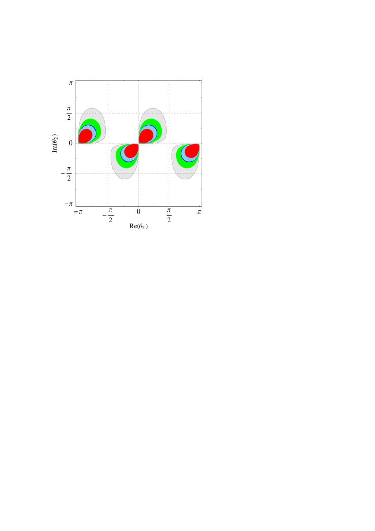
(a) $\quad\quad T_{\mathrm{RH}}\leq 2\times 10^{10}\,\text{GeV},\,\quad\quad$ $\quad\quad\theta_{13}=\delta=\varphi_{1}=\varphi_{2}=0^{\circ}$

(b) $\quad\quad T_{\mathrm{RH}}\leq 2\times 10^{10}\,\text{GeV},\,\quad\quad$ $\theta_{13}=\delta=\varphi_{1}=\varphi_{2}=0^{\circ}$

(c) $\quad\quad T_{\mathrm{RH}}\leq 5\times 10^{9}\,\text{GeV},\,\quad\quad$ $\theta_{13}=\delta=\varphi_{1}=\varphi_{2}=0^{\circ}$

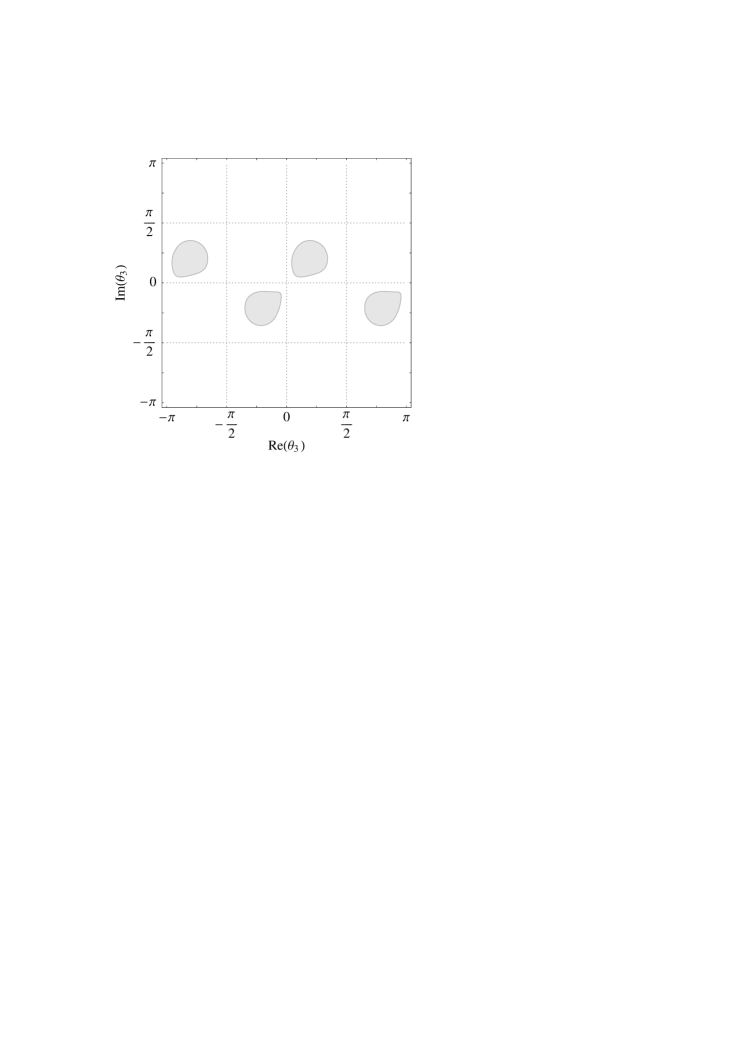
(d) $\quad\quad T_{\mathrm{RH}}\leq 5\times 10^{9}\,\text{GeV},\,\quad\quad$ $\theta_{13}=\delta=\varphi_{1}=\varphi_{2}=0^{\circ}$

Figure 5: Regions of $\mathrm{Re}(\theta_{2})-\mathrm{Im}(\theta_{2})$ and $\mathrm{Re}(\theta_{3})-\mathrm{Im}(\theta_{3})$ parameter spaces compatible with successful thermal leptogenesis in the presence of bounds on the reheat temperature: $T_{\mathrm{RH}}\leq 2\times 10^{10}$ GeV (upper panels) and $T_{\mathrm{RH}}\leq 5\times 10^{9}$ GeV (lower panels). From out- to inner-most regions, the associated ranges of maximally possible baryon asymmetry are: $n_{\text{B}}/n_{\gamma}\in[10^{-10},\,3\times 10^{-10}]$, $n_{\text{B}}/n_{\gamma}\in[3\times 10^{-10},\,5.9\times 10^{-10}]$, $n_{\text{B}}/n_{\gamma}\in[5.9\times 10^{-10},\,6.3\times 10^{-10}]$, $n_{\text{B}}/n_{\gamma}\in[6.3\times 10^{-10},\,10^{-9}]$ and $n_{\text{B}}/n_{\gamma}\gtrsim 10^{-9}$. The corresponding colour code is grey, green, dark blue (WMAP), light blue and red.

In Fig. 6 we illustrate the effects of non-zero $\theta_{1}$. Taking $\mbox{arg}(\theta_{2})=\mbox{arg}(\theta_{3})=\pi/4$, and again $\theta_{13},\delta,\varphi_{1},\varphi_{2}=0^{\circ}$, we now display the regions of the $\mathrm{Re}(\theta_{2})-\mathrm{Re}(\theta_{3})$ parameter space compatible with thermal leptogenesis in the presence of a bound $T_{\mathrm{RH}}\leq 5\times 10^{9}$ GeV. First, let us point out that Fig. 6(a) corresponds to a variation of Figs. 5(c) and (d), but for fixed values of $\mbox{arg}(\theta_{2})$ and $\mbox{arg}(\theta_{3})$. When compared to Fig. 6(a), Fig. 6(b) shows the effect of $\theta_{1}=\pi/4$, which is mainly a rotation (and a slight deformation) of the allowed region. Figure 6(c) and Fig. 6(d) illustrate that an imaginary part of $\theta_{1}$, in addition to introducing an additional source of CP violation, leads to a reduction of the compatible parameter space. As argued in Section 4.2.1, this effect can be explained by a stronger washout due to an enhancement of the parameters $\widetilde{m}_{1,\alpha}$. We emphasise that for complex $\theta_{i}$ (but vanishing low-energy CP phases), even in the presence of non-zero values of $\theta_{1}$, small values of $|s_{2}|$ and $|s_{3}|$ are still favoured by thermal leptogenesis.

(a) $T_{\mathrm{RH}}\leq 5\times 10^{9}\,\text{GeV},\,\mbox{arg}(\theta_{2},\theta_{3})=\pi/4,$ $\theta_{1}=0$

(b) $T_{\mathrm{RH}}\leq 5\times 10^{9}\,~{}\text{GeV},\,\mbox{arg}(\theta_{2},\theta_{3})=\pi/4,$ $|\theta_{1}|=\pi/4,\,~{}\mbox{arg}(\theta_{1})=0$

(c) $T_{\mathrm{RH}}\leq 5\times 10^{9}\,~{}\text{GeV},\,\mbox{arg}(\theta_{2},\theta_{3})=\pi/4,$ $|\theta_{1}|=\pi/4,\,~{}\mbox{arg}(\theta_{1})=\pi/8$

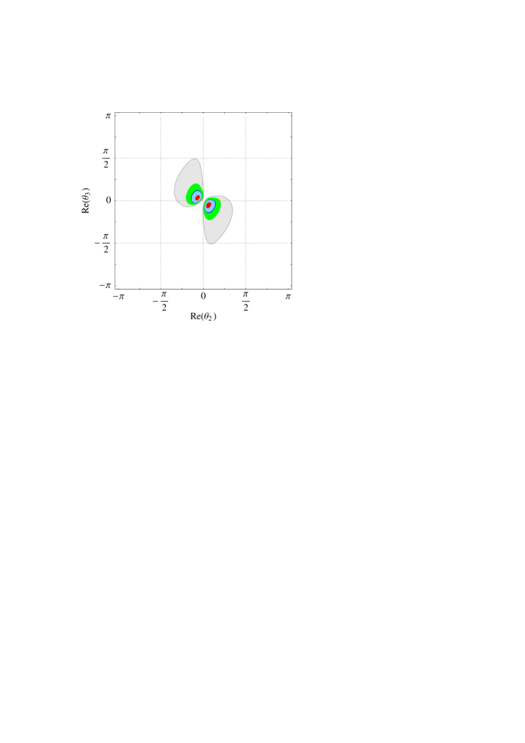
(d) $T_{\mathrm{RH}}\leq 5\times 10^{9}\,~{}\text{GeV},\,\mbox{arg}(\theta_{2},\theta_{3})=\pi/4,$ $|\theta_{1}|=\pi/4,\,~{}\mbox{arg}(\theta_{1})=\pi/4$

Figure 6: Regions of $\mathrm{Re}(\theta_{2})-\mathrm{Re}(\theta_{3})$ parameter space compatible with successful thermal leptogenesis in the presence of a bound $T_{\mathrm{RH}}\leq 5\times 10^{9}$ GeV. We display several values of complex $\theta_{1}$, choosing $\mbox{arg}(\theta_{2})=\mbox{arg}(\theta_{3})=\pi/4$ and $\theta_{13}=\delta=\varphi_{1}=\varphi_{2}=0^{\circ}$. Colour code as in Fig. 5.

In Fig. 5 we have separately considered the effects of each of the $R$-matrix angles $\theta_{2,3}$, while in Fig. 6 we analysed the impact of non-vanish $\theta_{1}$ upon the $\mathrm{Re}(\theta_{2})-\mathrm{Re}(\theta_{3})$ parameter space, assuming sizable arguments for both $\theta_{2}$ and $\theta_{3}$. However, for quite small values of the arguments, and when flavour effects are taken into account, new interesting regions of the $\mathrm{Re}(\theta_{2})-\mathrm{Re}(\theta_{3})$ parameter space can also arise. This is shown in Fig. 7, where we now display the regions of the $\mathrm{Re}(\theta_{2})-\mathrm{Re}(\theta_{3})$ parameter space compatible with successful thermal leptogenesis, assuming a small value for both arguments, namely $\pi/16$.

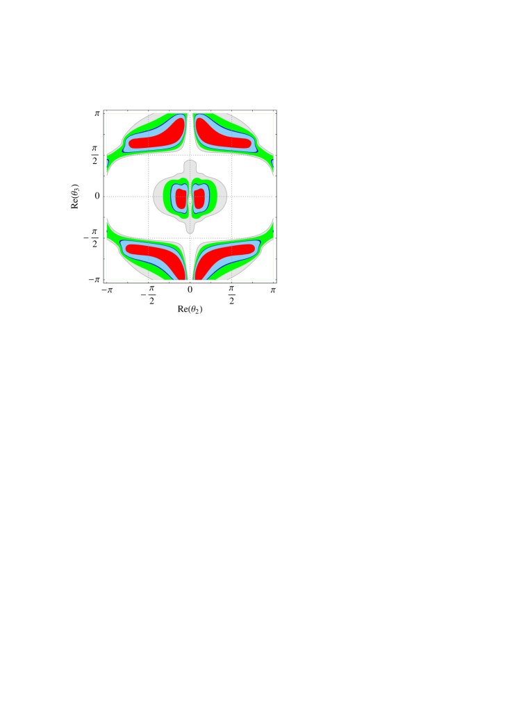
(a) $T_{\mathrm{RH}}\leq 2\times 10^{10}\>\mbox{GeV}\,,\,\,\theta_{1}=0\,,$ $\,\mbox{arg}(\theta_{2})=\mbox{arg}(\theta_{3})=\pi/16$

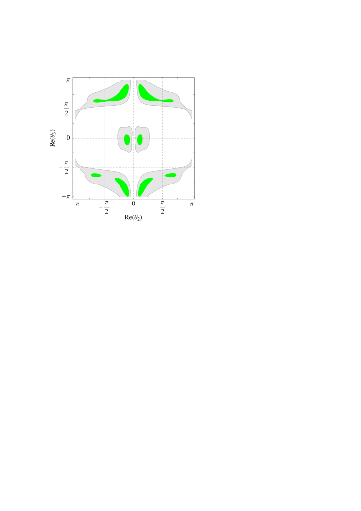
(b) $T_{\mathrm{RH}}\leq 5\times 10^{9}\>\mbox{GeV}\,,\,\,\theta_{1}=0\,,$ $\,\mbox{arg}(\theta_{2})=\mbox{arg}(\theta_{3})=\pi/16$

Figure 7: Regions of $\mathrm{Re}(\theta_{2})-\mathrm{Re}(\theta_{3})$ compatible with successful thermal leptogenesis. We take $\theta_{1}=0$, and consider $\arg(\theta_{2})=\arg(\theta_{3})=\pi/16$. $T_{\mathrm{RH}}\leq 2\times 10^{10}$ GeV in (a), while $T_{\mathrm{RH}}\leq 5\times 10^{9}$ GeV in (b). In this example we have set $\theta_{13}=\delta=\varphi_{1}=\varphi_{2}=0^{\circ}$. Colour code as in Fig. 5.

As can be seen, not only do we encounter large values of BAU associated with small values of $|s_{2}|$ and $|s_{3}|$, but new extensive regions, with larger values of $\theta_{2}$ and $\theta_{3}$, are now present. The origin of these new regions exhibiting a sizable BAU can be easily understood (in the limit of vanishing $\theta_{1}$) from the analytical considerations of Sections 4.2.1 and 4.2.2. On the one hand, Eqs. (28-30) show that optimal washout is possible in two cases: for large $s_{3}$, or then for large $s_{3}$ and $s_{2}$, provided that $c_{3}$ is small. On the other hand, from Eqs. (4.2.2-4.2.2) we have seen that optimal decay asymmetries require contributions from non-zero $\theta_{2}$, suppressed if $c_{3}$ is small. The shape of the extensive regions in Fig. 7(a) with sizable BAU reflects the balance between having a sufficiently small washout, while at the same time succeeding in obtaining an important decay asymmetry. As expected, taking into account stricter bounds on $T_{\text{RH}}$ leads to the disappearance of the WMAP compatible regions (c.f. Fig. 7(b)). Nevertheless, regions where the BAU is close to the observed range still survive, both for small and large $\theta_{2}$ and $\theta_{3}$. For non-vanishing values of $\theta_{1}$, just like discussed regarding Fig. 6, one would observe a deformation of the regions displayed in Fig. 7. The analytical interpretation can be now obtained from Eqs. (25-27), albeit in a less straightforward way.

After having revisited leptogenesis scenarios where CP violation originated solely from the complex $R$-matrix angles, let us now consider the effects of having CP violation arising from the $U_{\text{MNS}}$ phases. This is especially appealing given that, and contrary to the $R$-matrix angles, parameters like $\delta$ and $\theta_{13}$ are likely to be observable in neutrino oscillation experiments. Additionally, and as pointed out in Refs. [15, 16] (although in the context of the SM), these are examples of scenarios where there is a maximal connection between leptogenesis and low-energy CP violation. We begin by addressing a scenario where the $R$-matrix angles are real (but non-zero) and $\delta$ is the only source of CP violation. For non-zero $\theta_{13}$ and $\delta$, Fig. 8 illustrates the emergence of new regions in the $\mathrm{Re}(\theta_{2})-\mathrm{Re}(\theta_{3})$ parameter space, potentially compatible with thermal leptogenesis in the presence of a bound $T_{\mathrm{RH}}\leq 2\times 10^{10}$ GeV. In this example we have chosen $\theta_{1}=\varphi_{1}=\varphi_{2}=0^{\circ}$. Notice that in the flavour-independent approximation, leptogenesis would have been impossible for a real $R$-matrix. From Fig. 8, we find that for $\theta_{13}=11.5^{\circ}$ (the largest value experimentally allowed) and CP violating phase $\delta$ close to $\pi/2$ (which maximises the decay asymmetry $\varepsilon_{1,e}$), somewhat larger $\theta_{2}$ values could now be marginally allowed. In any case, the largest values of the BAU are still associated with small $\theta_{2}$ and $\theta_{3}$. On the other hand, moving away from the present upper bound on $\theta_{13}$, we find that the scenario is even more compromised. In fact, for $\theta_{13}=7.5^{\circ}$, only regions with BAU differing from the WMAP range by a factor 5 survive. For smaller $\theta_{13}$ values (namely $\theta_{13}\leq 5^{\circ}$), $n_{\text{B}}/n_{\gamma}$ is already well below $10^{-10}$. Likewise, considering stricter bounds on $T_{\mathrm{RH}}$ would lead to the disappearance of all the shaded regions of Fig. 8.

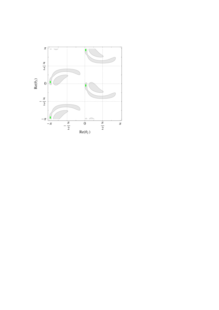
(a) $T_{\mathrm{RH}}\leq 2\times 10^{10}\,\text{GeV},\,\theta_{13}=11.5^{\circ},\delta=90^{\circ}$

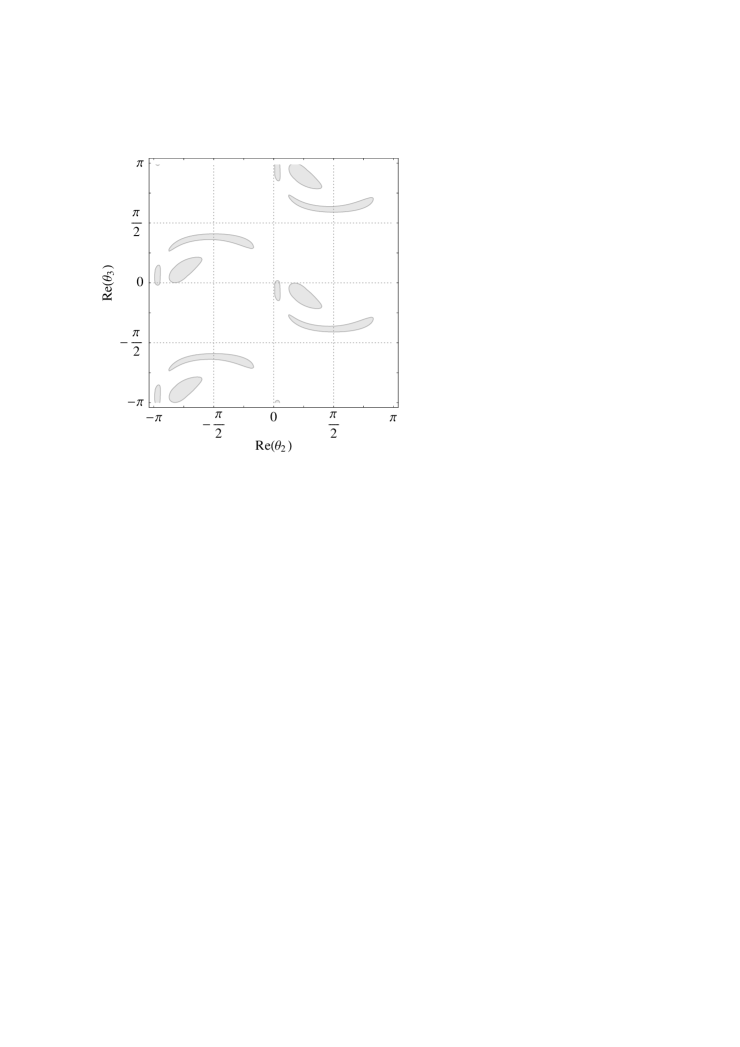
(b) $T_{\mathrm{RH}}\leq 2\times 10^{10}\,\text{GeV},\,\theta_{13}=7.5^{\circ},\delta=90^{\circ}$

Figure 8: Regions of $\mathrm{Re}(\theta_{2})-\mathrm{Re}(\theta_{3})$ parameter space compatible with successful thermal leptogenesis with a bound $T_{\mathrm{RH}}\leq 2\times 10^{10}$ GeV. In this example we have chosen real $R$-matrix angles and $\theta_{1}=\varphi_{1}=\varphi_{2}=0^{\circ}$. Colour code as in Fig. 5.

In Fig. 9, we display the effect of non-zero $\theta_{1}$ on the allowed regions with non-zero $\theta_{13}$ and $\delta$. In the first example with $\theta_{1}=\pi/4$ and $\theta_{13}=11.5^{\circ}$ (Fig. 9(a)), we observe that in addition to a rotation of the allowed parameter space, the latter is somewhat enlarged.

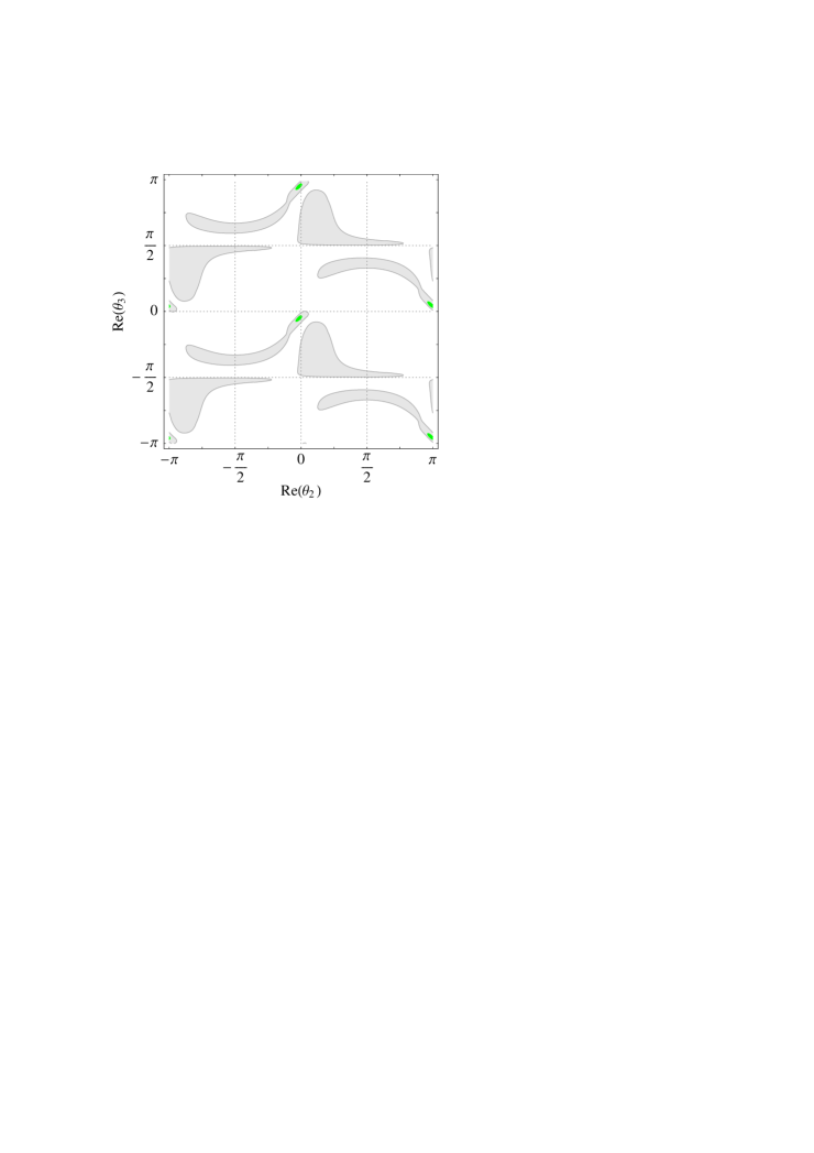
(a) Same input values as in Fig. 8(a), but $\theta_{1}=\pi/4$

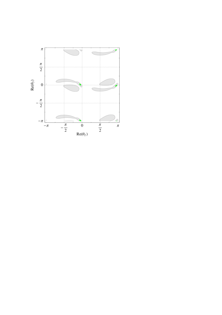
(b) Same input values as in Fig. 8(a), but $\theta_{1}=3\pi/4$

Figure 9: Example displayed in Figs. 8(a) and (c), but with $\theta_{1}\not=0^{\circ}$. Colour code as in Fig. 5.

At this point, and from the examples so far considered, we are led to the conclusion that, unless $\theta_{13}$ is found to be close to its present upper bound, it is quite difficult to accommodate viable BAU scenarios relying on $\delta$ as their only source of CP violation. For stricter bounds on the reheat temperature, the latter scenarios become increasingly more compromised.

In addition to $\delta$, there are other sources of CP violation arising from the $U_{\text{MNS}}$ matrix, namely the Majorana phases $\varphi_{1},\varphi_{2}$. In principle, the latter could also provide the required CP violation for leptogenesis (see also Refs. [13, 15, 16]). For completeness, in Fig. 10 we separately illustrate their role in generating a non-vanishing BAU. To do so, we assume a real $R$-matrix, $\delta=0^{\circ}$, and take $\varphi_{1(2)}=0^{\circ}$ on the left (right) panel. As seen from Fig. 10, when CP violation is exclusively arising from the Majorana phases it is indeed possible to obtain marginally compatible BAU values. Again, the most promising regions appear associated with small $\theta_{2}$ and $\theta_{3}$. We also observe that $\varphi_{1}$ and $\varphi_{2}$ lead to somewhat distinct regions on the $\mathrm{Re}(\theta_{2})-\mathrm{Re}(\theta_{3})$ parameter space. In this example we have again considered a more relaxed bound for the reheat temperature, $T_{\mathrm{RH}}\leq 2\times 10^{10}$ GeV. As occurred for the cases investigated in Fig. 8, stronger bounds on $T_{\text{RH}}$ would imply that the generated BAU would also lie below $10^{-10}$, so that the shaded regions of the $\mathrm{Re}(\theta_{2})-\mathrm{Re}(\theta_{3})$ parameter space displayed in Fig. 10 would disappear.

(a) $\quad\quad T_{\mathrm{RH}}\leq 2\times 10^{10}\,~{}\text{GeV},\,\varphi_{2}=180^{\circ},\,$ $\quad\theta_{13}=\delta=\varphi_{1}=0^{\circ}$

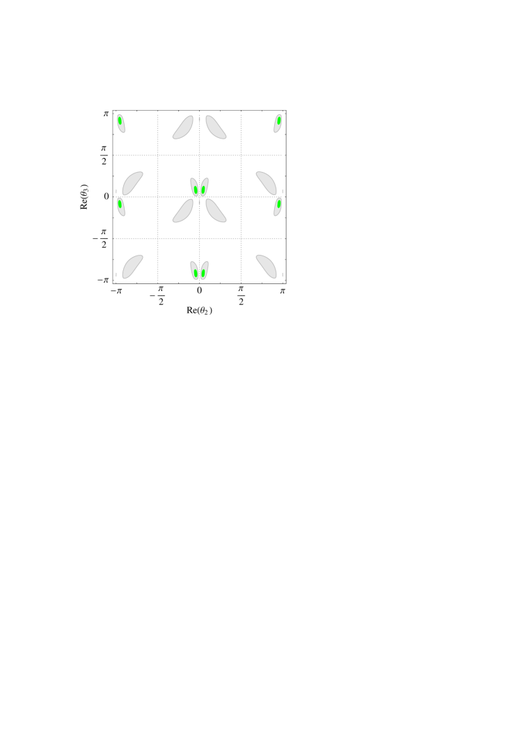
(b) $\quad\quad T_{\mathrm{RH}}\leq 2\times 10^{10}\,~{}\text{GeV},\,\varphi_{1}=180^{\circ},\,$ $\quad\theta_{13}=\delta=\varphi_{2}=0^{\circ}$

Figure 10: Regions of $\mathrm{Re}(\theta_{2})-\mathrm{Re}(\theta_{3})$ parameter space compatible with successful thermal leptogenesis with $T_{\mathrm{RH}}\leq 2\times 10^{10}$ GeV. In this example we have chosen real $R$, $\theta_{1}=0$ and $\theta_{13}=\delta=0^{\circ}$. Colour code as in Fig. 5.

Albeit it is pedagogical to consider the individual role of each $U_{\text{MNS}}$ phase regarding BAU, in the most general case $\delta$, $\varphi_{1}$ and $\varphi_{2}$ can be simultaneously non-vanishing. In fact, and as shown in Fig. 11, the Majorana phases can slightly improve the BAU allowed regions associated with $\delta$ (and $\theta_{13}$). We recall that, as discussed in relation with Fig. 8, values $\theta_{13}\leq 5^{\circ}$ failed to induce $n_{\text{B}}/n_{\gamma}>10^{-10}$. Comparing Fig. 11 with Fig. 8(c), we observe that for the choice of $\varphi_{1,2}=180^{\circ}$ the regions where $n_{\text{B}}/n_{\gamma}\in[3\times 10^{-10},\,5.9\times 10^{-10}]$ have become larger. Even though the WMAP range cannot be accounted for, it is nevertheless clear that the joint effect of the different $U_{\text{MNS}}$ phases translates in an improved scenario.

(a) $\quad T_{\mathrm{RH}}\leq 2\times 10^{10}\,\text{GeV},\,\varphi_{2}=180^{\circ},$ $\quad\theta_{13}=10^{\circ},\,\delta=90^{\circ},\,\varphi_{1}=0^{\circ}$

(b) $\quad T_{\mathrm{RH}}\leq 2\times 10^{10}\,\text{GeV},\,\varphi_{1}=180^{\circ},$ $\quad\theta_{13}=10^{\circ},\,\delta=90^{\circ},\,\varphi_{2}=0^{\circ}$

Figure 11: Same examples as in Fig. 10, but with $\theta_{13}=10^{\circ}$ and $\delta=90^{\circ}$.

Even though flavour-dependent thermal leptogenesis opens the possibility to generate the observed BAU exclusively from the $U_{\text{MNS}}$ CP violating phases, this may not be the most general nor the most successful scenario. The analysis of the present section lends a strong support to the latter statement. As we have found, it is quite difficult to encounter viable BAU scenarios associated with only low-energy CP violation. Moreover, if the given SUSY model implies a more stringent bound on the reheat temperature, BAU solely from $U_{\text{MNS}}$ phases becomes almost inviable.

Recall that in the most general case, the $R$-matrix angles are also complex and that, as seen from Figs. 5, 6 and 7, there are important regions in the $\theta_{2}$-$\theta_{3}$ parameter space where one can easily have compatibility with the WMAP range. In addition, $R$-matrix phases allow for viable BAU even under a bound $T_{\mathrm{RH}}\leq 5\times 10^{9}$ GeV. Thus, it is important to investigate the simultaneous effect of all CP violating phases. In particular, one wonders to which extent the $U_{\text{MNS}}$ phases can affect the BAU predictions from the $R$-matrix phases, and vice-versa.

In Fig. 12 we display the outcome of taking, in addition to the CP sources considered in Fig. 11, non-vanishing values for the arguments of $\theta_{2}$ and $\theta_{3}$, namely $\pi/16$ (upper) and $\pi/4$ (lower). The results are again depicted in the $\mathrm{Re}(\theta_{2})-\mathrm{Re}(\theta_{3})$ plane, and we assume two bounds for the reheat temperature, $T_{\mathrm{RH}}\leq 2\times 10^{10}$ GeV (left) and $T_{\mathrm{RH}}\leq 5\times 10^{9}$ GeV (right). It is manifest from the comparison of Fig. 7 with Fig. 12 that the predictions for the $\mathrm{Re}(\theta_{2})-\mathrm{Re}(\theta_{3})$ plane are hardly affected by considering non-vanishing values for the $U_{\mathrm{MNS}}$ phases. In the case of $\mbox{arg}(\theta_{2,3})=\pi/16$, and even for nearly maximal values of $\theta_{13}$, one only observes a small distortion of the regions associated with small $|s_{2}|$ and $|s_{3}|$, and a deformation of the regions associated with large $|s_{2}|$ and $|s_{3}|$ (c.f. Fig. 12(b)). For larger arguments of $\theta_{2}$ and $\theta_{3}$ ($\pi/4$), comparing Fig. 12(d) with Fig. 6(a) implies that $\theta_{13}$ and $\delta$ have had virtually no effect on the shape of the BAU compatible region, which is determined by the right-handed neutrino complex parameters $\theta_{2}$ and $\theta_{3}$. Finally, notice that for $T_{\mathrm{RH}}\leq 5\times 10^{9}$ GeV, it is possible to nearly reach the WMAP range for $\mbox{arg}(\theta_{2,3})$ as small as $\pi/16$. Assuming larger values for the arguments of the $R$-matrix angles allows to encounter wider regions where one still has compatibility with WMAP observations (panel (d)). However, this again favours the region of small $|s_{2}|$ and $|s_{3}|$.

In a sense, Fig. 12 provides an illustrative summary of our analysis. Firstly, it confirms the supposition that flavour effects in the Boltzmann equations indeed lead to the occurrence of new regions where BAU is viable (due to the already mentioned reduced washout). In addition, from its comparison to Fig. 6, it is also manifest that, in general, the leading role in BAU appears to be played by the $R$-matrix complex angles, and not by the $U_{\mathrm{MNS}}$ phases (which in turn may compromise the possible bridges that could otherwise be established between low-energy CP violation and BAU). Moreover, Fig. 12 is a clear example of the impact of the reheat temperature in severely constraining the SUSY seesaw parameters. The stricter the bounds on $T_{\mathrm{RH}}$, the more favoured are regions with small $\text{Re}(\theta_{2,3})$ and large $\mbox{arg}(\theta_{2,3})$.

(a) $\quad T_{\mathrm{RH}}\leq 2\times 10^{10}\>\mbox{GeV}\,,$ $\,\mbox{arg}(\theta_{2})=\mbox{arg}(\theta_{3})=\pi/16$

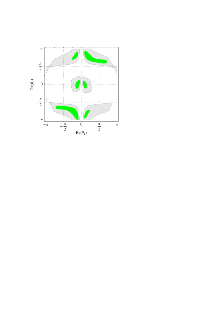
(b) $\quad T_{\mathrm{RH}}\leq 5\times 10^{9}\>\mbox{GeV}\,,$ $\,\mbox{arg}(\theta_{2})=\mbox{arg}(\theta_{3})=\pi/16$

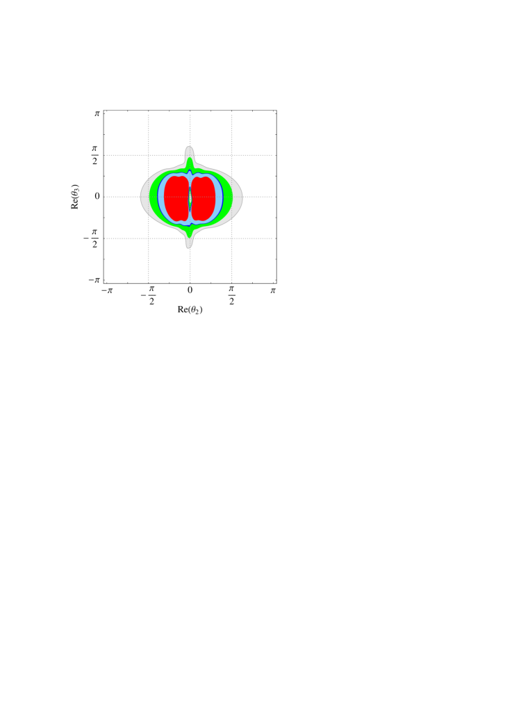
(c) $\quad T_{\mathrm{RH}}\leq 2\times 10^{10}\>\mbox{GeV}\,,$ $\,\mbox{arg}(\theta_{2})=\mbox{arg}(\theta_{3})=\pi/4$

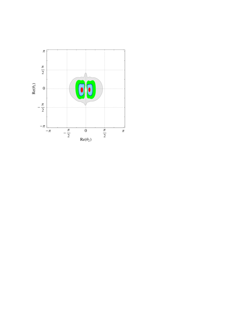
(d) $\quad T_{\mathrm{RH}}\leq 5\times 10^{9}\>\mbox{GeV}\,,$ $\,\mbox{arg}(\theta_{2})=\mbox{arg}(\theta_{3})=\pi/4$

Figure 12: Regions of $\mathrm{Re}(\theta_{2})-\mathrm{Re}(\theta_{3})$ parameter space compatible with successful thermal leptogenesis. We take $\theta_{13}=10^{\circ},\,\delta=90^{\circ},$ and $\varphi_{1}=180^{\circ}$. We consider $\arg(\theta_{2})=\arg(\theta_{3})=\pi/16$ for panels (a) and (b), and $\arg(\theta_{2})=\arg(\theta_{3})=\pi/4$ for panels (c) and (d). $T_{\mathrm{RH}}\leq 2\times 10^{10}$ GeV ((a) and (c)) while $T_{\mathrm{RH}}\leq 5\times 10^{9}$ GeV ((b) and (d)). Colour code as in Fig. 5.

5 Summary and conclusions

In this study we have investigated the constraints on the SUSY seesaw parameter space arising from flavour-dependent thermal leptogenesis in the MSSM in the presence of upper bounds on the reheat temperature of the early Universe. In the temperature range here considered, both tau- and muon-flavours are in thermal equilibrium, so that the full flavour-dependence was taken into account. In order to calculate the efficiency factor for thermal leptogenesis, we have extended the flavour-dependent Boltzmann equations [10, 11, 12], which were adapted to the MSSM case in [14], to include reheating (following Ref. [20]). Parameterising the solutions to the seesaw equation by means of a complex orthogonal matrix $R$ [7], we have analysed which regions of the seesaw parameter space generically enable optimal efficiency and/or optimal decay asymmetries for leptogenesis.

We have discussed several differences between the flavour-independent approximation and the correct flavour-dependent treatment of thermal leptogenesis. These are extensive, and, together with the bounds from the reheat temperature, lead to interesting new constraints on the SUSY seesaw parameter space.

Considerations on $T_{\text{RH}}$ give rise to the first constraints, in the sense that a dramatic drop in the efficiency takes place for $m_{N_{1}}\gg T_{\text{RH}}$ (as much as three orders of magnitude for $m_{N_{1}}\approx 10\,T_{\text{RH}}$). Since we have assumed that only the decays of the lightest right-handed neutrino were relevant for the lepton asymmetry, no bounds on the masses $m_{N_{2}}$ and $m_{N_{3}}$ were derived. Assuming an optimal regime for the decay asymmetry and for the efficiency, as well as that the inflaton only decays into MSSM particles (and not directly into right-handed (s)neutrinos), the requirement of a successful BAU leads to lower bounds on $m_{N_{1}}$ as well as on the reheat temperature. In particular, we have found $m_{N_{1}}^{\text{min}}\approx 1.5\times 10^{9}$ GeV and $T_{\text{RH}}^{\text{min}}\approx 1.9\times 10^{9}$ GeV, similar to the results obtained in the flavour-independent approximation [20]. On the other hand, in the presence of upper bounds on the reheat temperature (from dark matter relic abundance considerations), an upper bound on $m_{N_{1}}$ can also be inferred. In order to illustrate the impact of reheating, we have considered two examples for $T_{\text{RH}}$, corresponding to mildly and strongly constrained scenarios: $T_{\text{RH}}\lesssim 2\times 10^{10}$ GeV, and $T_{\text{RH}}\lesssim 5\times 10^{9}$ GeV. Regarding the upper bound on $m_{N_{1}}$, the latter bounds respectively yield $m^{\text{max}}_{N_{1}}\approx 1.4\times 10^{11}$ GeV, and $m^{\text{max}}_{N_{1}}\approx 1.9\times 10^{10}$ GeV. This leads to viability windows for the mass of the lightest right-handed neutrino.

Regarding the light neutrino masses, namely $m_{\nu_{1}}$, in general there is no upper bound from flavour-dependent thermal leptogenesis. Nevertheless, increasing $m_{\nu_{1}}$ within the present allowed experimental upper bounds (of roughly $0.5$ eV), generically results in a reduced BAU. Furthermore, in the presence of strong $T_{\text{RH}}$ bounds, quasi-degenerate light neutrino masses (via the type-I seesaw mechanism) become disfavoured.

As in the flavour-independent approximation, considerations on the washout parameters generically favour the region of small $|\sin\theta_{2}|$ and $|\sin\theta_{3}|$. However, and in clear contrast to the flavour-independent approximation, new regions with optimal flavour-dependent washout parameters have emerged, in association with large values of $|\sin\theta_{2}|$ and $|\sin\theta_{3}|$. In any case, in order to produce sufficient BAU in the presence of mild (or even strong) constraints on the reheat temperature, the decay asymmetries must also be close to their optimal values. Regarding the flavour-dependent decay asymmetries, in the general case of complex $R$ matrix (but considering the limit of a real $U_{\text{MNS}}$), we generically recovered the main results of the one-flavour computation (in the sense that the favoured regions still corresponded to small $|\sin\theta_{2}|$ and $|\sin\theta_{3}|$, albeit slightly enlarged). Another important result of our analysis concerns the effects of the reheat temperature, which were clearly manifest. In fact, taking stronger bounds on $T_{\text{RH}}$ leads to a significant reduction in the BAU allowed regions of the $\mathrm{Re}(\theta_{2})$-$\mathrm{Im}(\theta_{2})$ and $\mathrm{Re}(\theta_{3})$-$\mathrm{Im}(\theta_{3})$ parameter spaces (even to the disappearance of the WMAP compatible regions). In particular, for $T_{\text{RH}}\lesssim 5\times 10^{9}$ GeV, we have seen that $\theta_{3}$ cannot exclusively account for the observed WMAP results.

In flavour-dependent leptogenesis, a potentially important role can also be played by the $U_{\text{MNS}}$ phases. In principle, viable BAU scenarios could be obtained in the presence of a CP-conserving $R$-matrix, with the required amount of CP violation stemming either from the Dirac phase $\delta$, or from the Majorana phases $\varphi_{1}$ and $\varphi_{2}$. In the SM, this situation has been discussed in Refs. [15, 16]. However, the constraints on the seesaw parameters in the MSSM are expected to differ from the SM case, since for the temperatures (and values of $\tan\beta$) under consideration, all flavours are separately treated in the MSSM Boltzmann equations, whereas only the $\tau$-flavour is separately considered in the SM case.

Exclusively relying on the phase $\delta$ and on $\theta_{13}$ (under the standard parameterisation of the $U_{\text{MNS}}$ matrix) is a phenomenologically challenging choice, since these are the most likely (yet) unknown $U_{\text{MNS}}$ parameters to be experimentally measured. However, we have verified that even with $\delta=\pi/2$, for values of $\theta_{13}<11.5^{\circ}$ (the present experimental limit) the obtained values of the baryon asymmetry are only marginally compatible with observation (when large theoretical uncertainties are allowed for). By themselves, and even in the limit $\theta_{13}=0^{\circ}$, both Majorana phases, $\varphi_{1}$ and $\varphi_{2}$, could in principle account for BAU. However, and similar to $\delta$, only marginal consistency with observations can be reached. In both cases the impact of the reheating temperature becomes manifest, since lower values of $T_{\text{RH}}$ can render these scenarios inviable. We also note that in the presence of small $\mbox{arg}(\theta_{i})$, the BAU generated from CP violation in the right-handed sector dominates over the contributions from low-energy phases. Thus, the sensitivity to the $U_{\text{MNS}}$ CP violating phases is lost. In the limit of very strict bounds on the reheat temperature, one is thus compelled to take into account complex $R$ as an additional source of CP violation.

In summary, we have investigated which regions of the SUSY seesaw parameter space are favoured by flavour-dependent thermal leptogenesis, when bounds on the reheat temperature are taken into account. For mildly constrained $T_{\text{RH}}$ (e.g. $T_{\text{RH}}\lesssim 2\times 10^{10}$ GeV), compatibility with the BAU observed by WMAP can be obtained for extensive new regions of the $\theta_{2}$-$\theta_{3}$ parameter space, which were previously disfavoured in the flavour-independent approximation. On the other hand, focusing on (normal) hierarchical light and heavy neutrinos, the scenario where only CP violation from the $U_{\text{MNS}}$ is considered (real $R$), turns out to be only marginally consistent, even for $\theta_{13}=10^{\circ}$, and under mild bounds on $T_{\mathrm{RH}}$. Stricter $T_{\text{RH}}$ bounds (e.g. $T_{\text{RH}}\lesssim 5\times 10^{9}$ GeV) strongly motivate that CP is (also) violated in the right-handed neutrino sector. While extensive regions of the $\theta_{2}$-$\theta_{3}$ parameter space can produce BAU close to the WMAP range in this case, the favoured seesaw parameter space, clearly consistent with observations, is that of small values of $|\sin\theta_{2}|$ and $|\sin\theta_{3}|$.

Given the attractiveness of the mechanism of thermal leptogenesis, and the interesting constraints it can provide, it would be desirable to further refine the computation of the baryon asymmetry. Together with the expected improved bounds from LFV, electric dipole moments and other related observables, leptogenesis may offer valuable information on the right-handed neutrino masses and mixings.

Appendix

Appendix A Boltzmann equations with reheating

The efficiency factor for thermal leptogenesis introduced in Section 3 is calculated from the flavour-dependent Boltzmann equations [8, 10, 11, 12], generalised to the MSSM case [14]. Regarding reheating, one follows the simple, yet convenient approach of Ref. [20], where the effects of reheating are described by a single parameter, $T_{\text{RH}}$. The limitations of the several approaches were summarised in Section 3.1.3. In this appendix, aiming at completeness, we present some technical details.

The Boltzmann equations, with $z=m_{N_{1}}/T$, can be written as [14, 20]:

$$Z\,\frac{\mathrm{d}\rho_{\phi}}{\mathrm{d}z} = -\frac{3}{z}\,\rho_{\phi}-\frac{\Gamma_{\phi}}{H\,z}\,\rho_{\phi}\;,$$ (A.1)

$$Z\,X\,\frac{\mathrm{d}Y_{N_{1}}}{\mathrm{d}z} = \frac{3\,(Z-1)\,X}{z}\,Y_{N_{1}}\,-\,2K\,z\,\frac{K_{1}(z)}{K_{2}(z)}\,f_{1}(z)\,(Y_{N_{1}}-Y^{\mathrm{eq}}_{N_{1}})\;,$$ (A.2)

$$Z\,X\,\frac{\mathrm{d}Y_{\widetilde{N}_{1}}}{\mathrm{d}z} = \frac{3\,(Z-1)\,X}{z}\,Y_{\widetilde{N}_{1}}\,-\,2K\,z\,\frac{K_{1}(z)}{K_{2}(z)}\,f_{1}(z)\,(Y_{\widetilde{N}_{1}}-Y^{\mathrm{eq}}_{\widetilde{N}_{1}})\;,$$ (A.3)

$$Z\,X\,\frac{\mathrm{d}\hat{Y}_{\Delta_{\alpha}}}{\mathrm{d}z} = -\;2\,\varepsilon_{1,\alpha}\,K\,z\,\frac{K_{1}(z)}{K_{2}(z)}\,f_{1}(z)\,\left[(Y_{N_{1}}-Y^{\mathrm{eq}}_{N_{1}})\,+\,(Y_{\widetilde{N}_{1}}-Y^{\mathrm{eq}}_{\widetilde{N}_{1}})\right]$$

$$+\;\frac{3\,(Z-1)\,X}{z}\,Y_{\alpha}\;+\;K_{\alpha}\,z\,\frac{K_{1}(z)}{K_{2}(z)}\,f_{2}(z)\,\frac{\sum_{\beta}A_{\alpha\beta}\,\hat{Y}_{\Delta_{\beta}}}{Y^{\mathrm{eq}}_{\alpha}}\,(Y^{\mathrm{eq}}_{N_{1}}+Y^{\mathrm{eq}}_{\widetilde{N}_{1}})\;.$$

The above equations should be solved from $z=m_{N_{1}}/T^{\mathrm{max}}$ to “infinity” (i.e.  $z\gg 1$).

Let us now address each of the quantities appearing in Eqs. (A.1 - A). First of all, let us comment on the effects of reheating. $\rho_{\mathrm{R}}$ and $\rho_{\phi}$ are the radiation energy density and the energy density from the coherent oscillations of the reheating scalar field $\phi$. The reheating temperature is given by

$$T_{\mathrm{RH}}=\left(\frac{45\,\Gamma^{2}_{\phi}\,M^{2}_{\mathrm{Pl}}}{4\pi^{3}g_{*}}\right)^{\frac{1}{4}},$$ (A.5)

where $\Gamma_{\phi}$ is the decay rate of $\phi$, $M_{\mathrm{Pl}}$ is the Planck scale, and $g_{*}=228.75$ was already introduced in Eq. (11). During reheating, $\rho_{\phi}$ dominates over $\rho_{\mathrm{R}}$. In the Boltzmann equations, reheating is taken into account by means of

$$Z=1-\frac{\Gamma_{\phi}\,\rho_{\phi}}{4H\rho_{\mathrm{R}}}\;,$$ (A.6)

which is equal to $0$ when the maximal reheat temperature $T^{\mathrm{max}}$ is reached (corresponding to our initial conditions), and which becomes $1$ after reheating. In the limit $Z\to 1$ (and $X\to 1$ - see definition below, in Eq. (A.13)), we recover the MSSM equations without reheating, as given in [14]. At the maximal temperature $T^{\mathrm{max}}$, the energy density $\rho_{\phi}$ can be calculated from the condition $Z=0$, using $\rho_{\mathrm{R}}=(m_{N_{1}}/z)^{4}\,\pi^{2}g_{*}/30$ together with Eq. (A.12). Notice that Eq. (A.5) allows to extract $\Gamma_{\phi}$ (appearing in Eq. (A.1)) as a function of the reheat temperature,

$$\Gamma_{\phi}=\left(\frac{T_{\mathrm{RH}}^{4}}{M_{\mathrm{Pl}}^{2}}\frac{4\pi^{3}g^{*}}{45}\right)^{\frac{1}{2}}.$$ (A.7)

We would like to stress that in specific models of reheating after inflation, the prospects for leptogenesis could be significantly different. Nevertheless, this set of Boltzmann equations (Eqs. (A.1 - A)) simulates the generic constraints arising for thermal leptogenesis from bounds on the reheat temperature for a large class of scenarios.

$\hat{Y}_{\Delta_{\alpha}}$ are defined as $\hat{Y}_{\Delta_{\alpha}}=Y_{B}/3-Y_{L_{\alpha}}$, with $Y_{L_{\alpha}}$ being the total (particle and sparticle) lepton number densities for a flavour $\alpha$. $Y_{\alpha,\widetilde{\alpha}}$ are the densities of the (s)lepton doublets and $Y_{N_{1},\widetilde{N}_{1}}$ are the densities of the right-handed (s)neutrinos. The corresponding equilibrium number densities (in the Boltzmann approximation) are given by

$$Y^{\mathrm{eq}}_{\ell}\!\!\! \approx \!\!\!Y^{\mathrm{eq}}_{\widetilde{\ell}}\approx\frac{45\,\zeta(3)}{\pi^{4}g_{*}}\frac{3}{4}\;,\quad\quad Y^{\mathrm{eq}}_{N_{1}}(z)\approx Y^{\mathrm{eq}}_{\widetilde{N}_{1}}(z)\approx\frac{45\,\zeta(3)}{2\pi^{4}g_{*}}\frac{3}{4}\,z^{2}\,K_{2}(z)\;,$$ (A.8)

with $K_{2}(z)$ (and $K_{1}(z)$) being the modified Bessel functions of the second kind.

The matrix $A$, which appears in the washout term in Eq. (A), is defined via the relation $\hat{Y}_{\alpha}=\sum_{\beta}A_{\alpha\beta}\,\hat{Y}_{\Delta_{\alpha}}$, with $\hat{Y}_{\alpha}\equiv Y_{\alpha}+Y_{\widetilde{\alpha}}$ being the combined densities for lepton and slepton doublets. Below $(1+\tan^{2}\beta)\times 10^{9}$ GeV, where the Boltzmann equations are solved for the individual asymmetries $\hat{Y}_{\Delta_{e}}$, $\hat{Y}_{\Delta_{\mu}}$ and $\hat{Y}_{\Delta_{\tau}}$, $A$ is given by [14]

$$A^{\mathrm{MSSM}}=\begin{pmatrix}-93/110&6/55&6/55\\ 3/40&-19/30&1/30\\ 3/40&1/30&-19/30\end{pmatrix}.$$ (A.9)

The final lepton asymmetry in each flavour is governed by $T_{\mathrm{RH}}$ and by three sets of parameters: $\varepsilon_{1,\alpha},K_{\alpha}$ and $K$. The parameters $\varepsilon_{1,\alpha}$, $\varepsilon_{1,\widetilde{\alpha}}$, $\varepsilon_{\widetilde{1},\alpha}$ and $\varepsilon_{\widetilde{1},\widetilde{\alpha}}$ denote the asymmetries for the decays of neutrino into Higgs and lepton, neutrino into Higgsino and slepton, sneutrino into Higgsino and lepton, and sneutrino into Higgs and slepton, respectively. They are defined as

$$\varepsilon_{1,\alpha}\!\!\! = \!\!\!\frac{\Gamma_{N_{1}\ell_{\alpha}}-\Gamma_{N_{1}\overline{\ell}_{\alpha}}}{\sum_{\alpha}(\Gamma_{N_{1}\ell_{\alpha}}+\Gamma_{N_{1}\overline{\ell}_{\alpha}})}\;,\quad\varepsilon_{1,\widetilde{\alpha}}=\frac{\Gamma_{N_{1}\widetilde{\ell}_{\alpha}}-\Gamma_{N_{1}\widetilde{\ell}_{\alpha}^{*}}}{\sum_{\alpha}(\Gamma_{N_{1}\widetilde{\ell}_{\alpha}}+\Gamma_{N_{1}\widetilde{\ell}_{\alpha}^{*}})}\;,$$

$$\varepsilon_{\widetilde{1},\alpha}\!\!\! = \!\!\!\frac{\Gamma_{\widetilde{N}^{*}_{1}\ell_{\alpha}}-\Gamma_{\widetilde{N}_{1}\overline{\ell}_{\alpha}}}{\sum_{\alpha}(\Gamma_{\widetilde{N}^{*}_{1}\ell_{\alpha}}+\Gamma_{\widetilde{N}_{1}\overline{\ell}_{\alpha}})}\;,\quad\varepsilon_{\widetilde{1},\widetilde{\alpha}}=\frac{\Gamma_{\widetilde{N}_{1}\widetilde{\ell}_{\alpha}}-\Gamma_{\widetilde{N}^{*}_{1}\widetilde{\ell}_{\alpha}^{*}}}{\sum_{\alpha}(\Gamma_{\widetilde{N}_{1}\widetilde{\ell}_{\alpha}}+\Gamma_{\widetilde{N}^{*}_{1}\widetilde{\ell}_{\alpha}^{*}})}\;,$$ (A.10)

with $\Gamma$ the decay rates of (s)neutrinos with (s)leptons in the final states. In the MSSM, the four decay asymmetries are equal, $\varepsilon_{1,\alpha}=\varepsilon_{1,\widetilde{\alpha}}=\varepsilon_{\widetilde{1},\alpha}=\varepsilon_{\widetilde{1},\widetilde{\alpha}}$, and given by Eq. (12). The parameters $K_{\alpha}$ control the washout processes for the asymmetry in an individual lepton flavour $\alpha$, and $K$ controls the source of right-handed neutrinos in the thermal bath. In analogy to the case without reheating, they are given by

$$K_{\alpha}\equiv\frac{\Gamma_{N_{1}\ell_{\alpha}}+\Gamma_{N_{1}\overline{\ell}_{\alpha}}}{H_{0}(m_{N_{1}})}\;,\quad K\equiv\sum_{\alpha}K_{\alpha}\;,\quad K_{\alpha}=K\frac{(\lambda_{\nu}^{\dagger})_{1\alpha}(\lambda_{\nu})_{\alpha 1}}{(\lambda_{\nu}^{\dagger}\lambda_{\nu})_{11}}\;,$$ (A.11)

where $H_{0}(m_{N_{1}})$ is the “fictitious” Hubble parameter (without reheating). The latter is computed without taking into account $\rho_{\phi}$ at $T=m_{N_{1}}$, and is given by $H_{0}(m_{N_{1}})\approx 1.66\sqrt{g_{*}}m_{N_{1}}^{2}/M_{\mathrm{Pl}}$. In the presence of $\rho_{\phi}$, the Hubble parameter is modified to

$$H=\left[\frac{8\pi}{3}(\rho_{\mathrm{R}}+\rho_{\phi})\right]^{\frac{1}{2}}\frac{1}{M_{\mathrm{Pl}}}\;,$$ (A.12)

and in order to match the $H$ (real) and $H_{0}$ (“fictitious”) Hubble parameters, one introduces the quantity $X$,

$$X\equiv\left(\frac{{\rho_{\mathrm{R}}+\rho_{\phi}}}{{\rho_{\mathrm{R}}}}\right)^{\frac{1}{2}}\,.$$ (A.13)

We further notice that the parameters $K_{\alpha}$ are related to $\widetilde{m}_{1,\alpha}$, introduced in Eq. (15), as

$$\widetilde{m}_{1,\alpha}=K_{\alpha}\,m^{*},\;\mbox{with}\;m^{*}\approx\sin^{2}(\beta)\times 1.58\times 10^{-3}\ {\rm eV}\,\,\cite[cite]{[\@@bibref{}{Antusch:2006cw}{}{}]}\,.$$ (A.14)

Finally, the function $f_{1}(z)$ accounts for the presence of $\Delta L=1$ scatterings and $f_{2}(z)$ accounts for scatterings in the washout term of the asymmetry. They are defined as

$$\gamma_{D}+\gamma_{\mathrm{S},\Delta L=1}\equiv\gamma_{D}f_{1}\;,\quad\frac{\gamma^{\alpha}_{D}}{2}+\gamma^{\alpha}_{\mathrm{W},\Delta L=1}\equiv\gamma^{\alpha}_{D}f_{2}\;,$$ (A.15)

where $\gamma_{D}$ is the thermally averaged total decay rate of $N_{1}$ and $\gamma_{\mathrm{S},\Delta L=1}$ represents the rates for the $\Delta L=1$ scattering. The corresponding flavour-dependent rates for washout processes involving the lepton flavour $\alpha$ are denoted by $\gamma^{\alpha}_{D}$ (from inverse decays involving leptons $\ell_{\alpha}$) and $\gamma^{\alpha}_{\mathrm{W},\Delta L=1}$.

References

- [1] D. N. Spergel et al., arXiv:astro-ph/0603449.
- [2] V. A. Kuzmin, V. A. Rubakov and M. E. Shaposhnikov, Phys. Lett. B 155 (1985) 36.
- [3] P. Minkowski, Phys. Lett. B 67 (1977) 421; M. Gell-Mann, P. Ramond and R. Slansky, in Complex Spinors and Unified Theories eds. P. Van. Nieuwenhuizen and D. Z. Freedman, Supergravity (North-Holland, Amsterdam, 1979), p.315 [Print-80-0576 (CERN)]; T. Yanagida, in Proceedings of the Workshop on the Unified Theory and the Baryon Number in the Universe, eds. O. Sawada and A. Sugamoto (KEK, Tsukuba, 1979), p.95; S. L. Glashow, in Quarks and Leptons, eds. M. Lévy et al. (Plenum Press, New York, 1980), p.687; R. N. Mohapatra and G. Senjanović, Phys. Rev. Lett. 44 (1980) 912.
- [4] R. Barbieri, D. V. Nanopolous, G. Morchio and F. Strocchi, Phys. Lett. B 90 (1980) 91; R. E. Marshak and R. N. Mohapatra, Invited talk given at Orbis Scientiae, Coral Gables, Fla., Jan. 14-17, 1980, VPI-HEP-80/02; T. P. Cheng and L. F. Li, Phys. Rev. D 22 (1980) 2860; M. Magg and C. Wetterich, Phys. Lett. B 94 (1980) 61; G. Lazarides, Q. Shafi and C. Wetterich, Nucl. Phys. B181 (1981) 287; J. Schechter and J. W. F. Valle, Phys. Rev. D 22 (1980) 2227; R. N. Mohapatra and G. Senjanović, Phys. Rev. D 23 (1981) 165.
- [5] M. Fukugita and T. Yanagida, Phys. Lett. B 174 (1986) 45.
- [6] For a review containing an extensive list of references, see e.g.: W. Buchmüller, R. D. Peccei and T. Yanagida, Ann. Rev. Nucl. Part. Sci. 55 (2005) 311 [arXiv:hep-ph/0502169].
- [7] J. A. Casas and A. Ibarra, Nucl. Phys. B 618 (2001) 171 [arXiv:hep-ph/0103065].
- [8] R. Barbieri, P. Creminelli, A. Strumia and N. Tetradis, Nucl. Phys. B 575 (2000) 61 [arXiv:hep-ph/9911315].
- [9] T. Endoh, T. Morozumi and Z. h. Xiong, Prog. Theor. Phys. 111 (2004) 123 [arXiv:hep-ph/0308276]; T. Fujihara, S. Kaneko, S. Kang, D. Kimura, T. Morozumi and M. Tanimoto, Phys. Rev. D 72 (2005) 016006 [arXiv:hep-ph/0505076].
- [10] A. Abada, S. Davidson, F. X. Josse-Michaux, M. Losada and A. Riotto, JCAP 0604 (2006) 004 [arXiv:hep-ph/0601083].
- [11] E. Nardi, Y. Nir, E. Roulet and J. Racker, JHEP 0601 (2006) 164 [arXiv:hep-ph/0601084].
- [12] A. Abada, S. Davidson, A. Ibarra, F. X. Josse-Michaux, M. Losada and A. Riotto, arXiv:hep-ph/0605281.
- [13] S. Blanchet and P. Di Bari, arXiv:hep-ph/0607330.
- [14] S. Antusch, S. F. King and A. Riotto, arXiv:hep-ph/0609038.
- [15] S. Pascoli, S. T. Petcov and A. Riotto, arXiv:hep-ph/0609125.
- [16] G. C. Branco, R. G. Felipe and F. R. Joaquim, arXiv:hep-ph/0609297.
- [17] S. Pascoli, S. T. Petcov and W. Rodejohann, Phys. Lett. B 549 (2002) 177 [arXiv:hep-ph/0209059]; S. Pascoli, S. T. Petcov and T. Schwetz, Nucl. Phys. B 734 (2006) 24 [arXiv:hep-ph/0505226].
- [18] For example, see: J. R. Ellis and M. Raidal, Nucl. Phys. B 643 (2002) 229 [arXiv:hep-ph/0206174]; J. R. Ellis, M. Raidal and T. Yanagida, Phys. Lett. B 546 (2002) 228 [arXiv:hep-ph/0206300]; S. Pascoli, S. T. Petcov and C. E. Yaguna, Phys. Lett. B 564 (2003) 241 [arXiv:hep-ph/0301095]; S. Kanemura, K. Matsuda, T. Ota, T. Shindou, E. Takasugi and K. Tsumura, Phys. Rev. D 72 (2005) 093004 [arXiv:hep-ph/0501228]; S. Kanemura, K. Matsuda, T. Ota, T. Shindou, E. Takasugi and K. Tsumura, Phys. Rev. D 72 (2005) 055012 [Erratum-ibid. D 72 (2005) 059904] [arXiv:hep-ph/0507264]; S. T. Petcov, T. Shindou and Y. Takanishi, Nucl. Phys. B 738 (2006) 219 [arXiv:hep-ph/0508243]; S. T. Petcov, W. Rodejohann, T. Shindou and Y. Takanishi, Nucl. Phys. B 739 (2006) 208 [arXiv:hep-ph/0510404]; F. Deppisch, H. Pas, A. Redelbach and R. Ruckl, Phys. Rev. D 73 (2006) 033004 [arXiv:hep-ph/0511062].
- [19] S. Antusch, E. Arganda, M. J. Herrero and A. M. Teixeira, arXiv:hep-ph/0607263.
- [20] G. F. Giudice, A. Notari, M. Raidal, A. Riotto and A. Strumia, Nucl. Phys. B 685 (2004) 89 [arXiv:hep-ph/0310123].
- [21] S. Davidson and A. Ibarra, Phys. Lett. B 535 (2002) 25 [arXiv:hep-ph/0202239].
- [22] A. H. Guth, Phys. Rev. D 23 (1981) 347; A. D. Linde, Phys. Lett. B 108 (1982) 389; A. Albrecht and P. J. Steinhardt, Phys. Rev. Lett. 48 (1982) 1220. For a review containing an extensive list of references, see also: D. H. Lyth and A. Riotto, Phys. Rept. 314 (1999) 1 [arXiv:hep-ph/9807278].
- [23] L. Covi, E. Roulet and F. Vissani, Phys. Lett. B 384 (1996) 169 [arXiv:hep-ph/9605319].
- [24] M. Flanz, E. A. Paschos, U. Sarkar and J. Weiss, Phys. Lett. B 389 (1996) 693; A. Pilaftsis, Phys. Rev. D 56 (1997) 5431. For recent works where flavour effects are taken into account, see e.g.: A. Pilaftsis and T. E. J. Underwood, Phys. Rev. D 72 (2005) 113001 [arXiv:hep-ph/0506107]; G. C. Branco, A. J. Buras, S. Jager, S. Uhlig and A. Weiler, arXiv:hep-ph/0609067.
- [25] O. Vives, Phys. Rev. D 73 (2006) 073006 [arXiv:hep-ph/0512160].
- [26] See e.g.: G. Lazarides and Q. Shafi, Phys. Lett. B 258 (1991) 305; H. Murayama and T. Yanagida, Phys. Lett. B 322 (1994) 349 [arXiv:hep-ph/9310297]; K. Hamaguchi, H. Murayama and T. Yanagida, Phys. Rev. D 65 (2002) 043512 [arXiv:hep-ph/0109030]; T. Moroi and H. Murayama, Phys. Lett. B 553 (2003) 126 [arXiv:hep-ph/0211019].
- [27] See e.g.: H. Murayama, H. Suzuki, T. Yanagida and J. Yokoyama, Phys. Rev. Lett. 70 (1993) 1912; J. R. Ellis, M. Raidal and T. Yanagida, Phys. Lett. B 581 (2004) 9 [arXiv:hep-ph/0303242]; S. Antusch, M. Bastero-Gil, S. F. King and Q. Shafi, Phys. Rev. D 71 (2005) 083519 [arXiv:hep-ph/0411298].
- [28] For recent discussions, see e.g.: R. Allahverdi and A. Mazumdar, arXiv:hep-ph/0603244; K. A. Olive and M. Peloso, arXiv:hep-ph/0608096; R. Allahverdi and A. Mazumdar, arXiv:hep-ph/0608296; R. Allahverdi, K. Enqvist, J. Garcia-Bellido, A. Jokinen and A. Mazumdar, arXiv:hep-ph/0610134.
- [29] W. Buchmüller, P. Di Bari and M. Plümacher, Annals Phys. 315 (2005) 305 [arXiv:hep-ph/0401240].
- [30] A. Pilaftsis and T. E. J. Underwood, Nucl. Phys. B 692 (2004) 303 [arXiv:hep-ph/0309342].
- [31] W. Buchmüller and M. Plümacher, Phys. Lett. B 511 (2001) 74 [arXiv:hep-ph/0104189].
- [32] S. Antusch, J. Kersten, M. Lindner and M. Ratz, Nucl. Phys. B 674 (2003) 401[arXiv:hep-ph/0305273].
- [33] S. Antusch, J. Kersten, M. Lindner, M. Ratz and M. A. Schmidt, JHEP 0503 (2005) 024 [arXiv:hep-ph/0501272].
- [34] W.-M. Yao et al. [Particle Data Group Collaboration], J. Phys. G 33 (2006) 1.
- [35] A recent discussion of possible differences between both treatments can be found in: M. Lindner and M. M. Muller, Phys. Rev. D 73 (2006) 125002 [arXiv:hep-ph/0512147].
- [36] M. Y. Khlopov and A. D. Linde, Phys. Lett. B 138 (1984) 265; J. R. Ellis, J. E. Kim and D. V. Nanopoulos, Phys. Lett. B 145 (1984) 181; J. R. Ellis, D. V. Nanopoulos and S. Sarkar, Nucl. Phys. B 259 (1985) 175; T. Moroi, H. Murayama and M. Yamaguchi, Phys. Lett. B 303 (1993) 289; M. Kawasaki, K. Kohri and T. Moroi, Phys. Lett. B 625 (2005) 7 [arXiv:astro-ph/0402490].
- [37] For a recent discussion, see: K. Kohri, T. Moroi and A. Yotsuyanagi, Phys. Rev. D 73 (2006) 123511 [arXiv:hep-ph/0507245].
- [38] For thermal production of gravitinos, see e.g.: M. Bolz, A. Brandenburg and W. Buchmuller, Nucl. Phys. B 606 (2001) 518 [arXiv:hep-ph/0012052]; J. Pradler and F. D. Steffen, arXiv:hep-ph/0608344.
- [39] L. Roszkowski, R. Ruiz de Austri and K. Y. Choi, JHEP 0508 (2005) 080 [arXiv:hep-ph/0408227]; D. G. Cerdeño, K. Y. Choi, K. Jedamzik, L. Roszkowski and R. Ruiz de Austri, JCAP 0606 (2006) 005 [arXiv:hep-ph/0509275]; see also: F. D. Steffen, JCAP 0609 (2006) 001 [arXiv:hep-ph/0605306].
- [40] W. Buchmüller, L. Covi, J. Kersten and K. Schmidt-Hoberg, arXiv:hep-ph/0609142.
- [41] For our numerical analysis, we have used the global fit results from: M. Maltoni, T. Schwetz, M. A. Tortola and J. W. F. Valle, New J. Phys. 6 (2004) 122 [arXiv:hep-ph/0405172v5].
- [42] W. Buchmüller, P. Di Bari and M. Plümacher, Nucl. Phys. B 665 (2003) 445 [arXiv:hep-ph/0302092].
- [43] S. Antusch and S. F. King, Phys. Lett. B 597 (2004) 199 [arXiv:hep-ph/0405093].
- [44] S. Antusch and S. F. King, JHEP 0601 (2006) 117 [arXiv:hep-ph/0507333]; Phys. Lett. B 591 (2004) 104 [arXiv:hep-ph/0403053]; Nucl. Phys. B 705 (2005) 239 [arXiv:hep-ph/0402121].
- [45] For a summary and references, see e.g.: C. Aalseth et al. [Part of the APS Neutrino Study], arXiv:hep-ph/0412300.
- [46] S. F. King, arXiv:hep-ph/0610239.