1+1 Dimensional Hydrodynamics for High–energy
Heavy–ion Collisions

Abstract

A 1+1 dimensional hydrodynamical model in the light–cone coordinates is used to describe central heavy–ion collisions at ultrarelativistic bombarding energies. Deviations from Bjorken’s scaling are taken into account by choosing finite–size profiles for the initial energy density. The sensitivity of fluid dynamical evolution to the equation of state and the parameters of initial state is investigated. Experimental constraints on the total energy of produced particles are used to reduce the number of model parameters. Spectra of secondary particles are calculated assuming that the transition from the hydrodynamical stage to the collisionless expansion of matter occurs at a certain freeze–out temperature. An important role of resonances in the formation of observed hadronic spectra is demonstrated. The calculated rapidity distributions of pions, kaons and antiprotons in central Au+Au collisions at $\sqrt{s_{\scriptscriptstyle NN}}=200$ GeV are compared with experimental data of the BRAHMS Collaboration. Parameters of the initial state are reconstructed for different choices of the equation of state. The best fit of these data is obtained for a soft equation of state and Gaussian–like initial profiles of the energy density, intermediate between the Landau and Bjorken limits.

I Introduction

High–energy heavy–ion collisions provide a unique tool for studying properties of hot and dense strongly–interacting matter in the laboratory. The theoretical description of such collisions is often done within the framework of a hydrodynamic approach. This approach opens the possibility to study the sensitivity of collision dynamics and secondary particle distributions to the equation of state (EOS) of the produced matter. The two most famous realizations of this approach, which differ by the initial conditions, have been proposed by Landau Lan53 (full stopping) and Bjorken Bjo83 (partial transparency). In recent decades many versions of the hydrodynamic model were developed, ranging from simplified 1+1 Mel58 ; Tar77 ; Mis83 ; Bla87 ; Esk98 ; Moh03 and 2+1 dimensional models Bla87 ; Kol99 ; Bas00 ; Per00 ; Kol01 ; Tea01 of the Landau or Bjorken type to more sophisticated 3+1 dimensional models Sto80 ; Ris95a ; Non00 ; Hir02 ; Ham05 ; Non05 . One should also mention the multi–fluid models Ams78 ; Cla86 ; Bar87 ; Mis88 ; Kat93 ; Bra00 ; Ton03 which consider the whole collision process including the nuclear interpenetration stage. Recent theoretical investigations show that fluid–dynamical models give a very good description of many observables at the SPS and RHIC bombarding energies (see e.g. Ref. Sto05 ).

The 2+1 dimensional hydrodynamical models have been successfully applied Kol99 ; Bas00 ; Per00 ; Kol01 ; Tea01 to describe the $p_{T}$ distributions of mesons and their elliptic flow at midrapidity. These models assume a boost–invariant expansion Bjo83 of matter in the longitudinal (beam) direction and, therefore, cannot explain experimental data in a broad rapidity region, where strong deviations from the scaling regime have been observed. More realistic 3+1 dimensional fluid–dynamical simulations have been already performed for heavy–ion collisions at SPS and RHIC energies. But as a rule, the authors of these models do not study the sensitivity of results to the choice of initial and final (freeze–out) stages. On the other hand, it is not clear at present, which initial conditions, Landau–like Lan53 or Bjorken–like Bjo83 , are more appropriate for ultrarelativistic collisions.

Our main goal in this paper is to see how well the fluid–dynamical approach describes the RHIC data on $\pi,K,\overline{p}$ distributions over a broad rapidity interval, reported recently by the BRAHMS Collaboration Bea04 ; Bea05 . Within our approach we explicitly impose a constraint on the total energy of the produced particles which follows from these data.

For our study we apply a simplified version of the hydrodynamical model, dealing only with the longitudinal dynamics of the fluid. This approach has as its limiting cases the Landau and Bjorken models. We investigate the sensitivity of the hadron rapidity spectra to the fluid’s equation of state, to the choice of initial state and freeze–out conditions. Modification of these spectra due to the feeding from resonance decays is also analyzed. Special attention is paid to possible manifestations of the deconfinement phase transition. In particular, we compare the dynamical evolution of the fluid with and without the phase transition.

The paper is organized as follows: in Sect. II we formulate the model and specify the equation of state, the initial and freeze-out conditions. In this section we also explain how we calculate particle spectra and take into account feeding from resonance decays. In Sect. III we present the numerical results. We first consider the evolution of fluid–dynamical profiles for different equations of states and initial conditions. Then these results are used to calculate spectra of pions, kaons and antiprotons. In the end of this section we analyze the initial conditions motivated by the Landau and Bjorken models. Summary and outlook are given in Sect. IV. Some details of numerical scheme and the procedure to calculate feeding from resonance decays are given in Appendix.

A short version of this paper is published in Ref. Sat06 .

II Formulation of the model

II.1 Equations of ideal fluid dynamics

Below we study the evolution of highly excited, and possibly deconfined, strongly–interacting matter produced in ultrarelativistic heavy–ion collisions. It is assumed that after a certain thermalization stage this evolution can be described by the relativistic fluid dynamics. Conservation laws of the baryon charge and 4–momentum are expressed by the following differential equations Lan59 :

$$\partial_{\mu}\left(n\hskip 1.0ptU^{\mu}\right)=0\,,$$ (1)

$$\partial_{\nu}T^{\mu\nu}=0\,,$$ (2)

where $n,U^{\mu}$ and $T^{\mu\nu}$ are the rest–frame baryon number density, the collective 4–velocity and the energy–momentum tensor of the fluid. In the limit of small dissipation, one can represent $T^{\mu\nu}$ in the standard form

$$T^{\mu\nu}=(\epsilon+P)\hskip 1.0ptU^{\mu}U^{\nu}-P\hskip 1.0ptg^{\mu\nu}.$$ (3)

Here $\epsilon$ and $P$ are the rest–frame energy density and pressure.

We consider central collisions of equal nuclei disregarding the effects of transverse collective expansion. In this case one can parametrize $U^{\mu}$ in terms of the longitudinal flow rapidity $Y$ as $U^{\mu}=(\cosh{Y},\bm{0},\sinh{Y})^{\mu}$. It is convenient to make transition from the usual space–time coordinates $t,z$ to the hyperbolic (light–cone) variables Bjo83 , namely, the proper time $\tau$ and the space–time rapidity $\eta$ , defined as

$$\tau=\sqrt{t^{2}-z^{2}}\,,\hskip 14.22636pt\eta=\tanh^{-1}\left(\frac{z}{t}\right)=\frac{1}{2}\ln{\frac{t+z}{t-z}}\,.$$ (4)

In these coordinates the equations (1)–(3) take the following form Bel96

$$\left[\tau\frac{\partial}{\partial\tau}+\tanh\hskip 1.0pt(Y-\eta)\hskip 1.0pt\frac{\partial}{\partial\eta}\right]\hskip 1.0ptn+n\left[\tanh\hskip 1.0pt(Y-\eta)\hskip 1.0pt\tau\frac{\partial}{\partial\tau}+\frac{\partial}{\partial\eta}\right]Y = 0\,,$$ (5)

$$\left[\tau\frac{\partial}{\partial\tau}+\tanh\hskip 1.0pt(Y-\eta)\hskip 1.0pt\frac{\partial}{\partial\eta}\right]\hskip 1.0pt\epsilon+(\epsilon+P)\left[\tanh\hskip 1.0pt(Y-\eta)\hskip 1.0pt\tau\frac{\partial}{\partial\tau}+\frac{\partial}{\partial\eta}\right]Y = 0\,,$$ (6)

$$(\epsilon+P)\left[\tau\frac{\partial}{\partial\tau}+\tanh\hskip 1.0pt(Y-\eta)\hskip 1.0pt\frac{\partial}{\partial\eta}\right]Y+\left[\tanh\hskip 1.0pt(Y-\eta)\hskip 1.0pt\tau\frac{\partial}{\partial\tau}+\frac{\partial}{\partial\eta}\right]P = 0\,.$$ (7)

To solve Eqs. (5)–(7), one needs to specify the EOS, $P=P\hskip 1.0pt(n,\epsilon)$, and the initial profiles $n\hskip 1.0pt(\tau_{0},\eta),\epsilon\hskip 1.0pt(\tau_{0},\eta),Y(\tau_{0},\eta)$ at a time $\tau=\tau_{0}$  when the fluid may be considered as thermodynamically equilibrated.

In this paper we consider only the baryon–free matter, i.e. assume vanishing net baryon density $n$ and chemical potential $\mu$. In this case Eq. (5) is trivially satisfied and all thermodynamic quantities, e.g. pressure, temperature $T$ and entropy density $s=(\epsilon+P-n\mu)/T$ , can be regarded as functions of $\epsilon$ only. The numerical solution of Eqs. (6)–(7) is obtained by using the relativistic version Ris95b of the flux–corrected transport algorithm Bor73 . The details of the computational procedure are given in Appendix A.

II.2 Initial conditions

Following Ref. Hir02 , we choose the initial conditions for a finite-size fluid, generalizing the Bjorken scaling conditions:

$$Y(\tau_{0},\eta)=\eta\,,\hskip 14.22636pt\epsilon\hskip 1.0pt(\tau_{0},\eta)=\epsilon_{0}\exp{\left[-\frac{(|\eta|-\eta_{0})^{2}}{2\sigma^{2}}\Theta(|\eta|-\eta_{0})\right]},$$ (8)

where $\Theta(x)\equiv(1+\textrm{sgn}\hskip 1.0ptx)/2$ . All calculations are performed for $\tau_{0}=1$ fm/c, assuming that $Y$ and $\epsilon$ are independent on the transverse coordinates. The particular choice $\eta_{0}=0$ corresponds to the pure Gaussian profile of the energy density. The case $\sigma=0$ corresponds to the ”table–like” profile when the initial energy density equals $\epsilon_{0}$ at $|\eta|<\eta_{0}$ and vanishes at larger $|\eta|$ . It is obvious that if $\sigma$ or $\eta_{0}$ tends to infinity, one gets the limiting case of the Bjorken scaling solution. In this case, as follows from Eqs. (5)–(7), $Y=\eta$ and $n,\epsilon,P$ are functions of $\tau$, determined by the ordinary differential equations Bjo83

$$\frac{d\hskip 1.0pt(n\tau)}{d\tau}=0\,,~{}~{}~{}\frac{d\hskip 1.0pt(\epsilon\tau)}{d\tau}+P=0\,.$$ (9)

Comparison of initial energy density profiles corresponding to the same total energy of produced particles, but having different parameters $\sigma$ and $\eta_{0}$, is made below in Fig. 5. The symmetry of central collisions of equal nuclei with respect to the transformation $z\to-z$ implies that at fixed $\tau$, including the initial state at $\tau=\tau_{0}$ , the flow rapidity and energy density should be, respectively, odd and even functions of $\eta$ :

$$Y\hskip 1.0pt(\tau,-\eta)=-Y\hskip 1.0pt(\tau,\eta)\,,~{}~{}~{}\epsilon\hskip 1.0pt(\tau,-\eta)=\epsilon\hskip 1.0pt(\tau,\eta)\,.$$ (10)

Therefore, it is sufficient to solve Eqs. (6)–(7) only in the forward ”hemisphere” $\eta\geqslant 0$ , using the boundary conditions $Y=0,\,\partial\epsilon/\partial\eta=0$ at $\eta=0$ .

II.3 Equation of state

One of the main goals of experiments on ultrarelativistic heavy–ion collisions is to study the deconfinement phase transition of strongly–interacting matter. In our calculations this phase transition is implemented through a bag–like EOS using the parametrization suggested in Ref. Tea01 . This EOS consists of three parts, denoted below by indices $H,M,Q$ , and corresponding, respectively, to the hadronic, ”mixed” and quark–gluon phases. As already mentioned, pressure, temperature and sound velocity, $c_{s}=\sqrt{dP/d\epsilon}$, of the baryon–free matter can be regarded as functions of $\epsilon$  only. It is further assumed that $c_{s}$ is constant in each phase and, therefore, $P$ is a linear function of $\epsilon$ with different slopes in the above–mentioned regions of energy density.

The hadronic phase corresponds to the domain of low energy densities, $\epsilon<\epsilon_{H}$, and temperatures, $T<T_{H}$ . This phase consists of pions, kaons, baryon–antibaryon pairs and hadronic resonances. Numerical calculations for the ideal gas of hadrons (see e.g. Cho05 ) predict a rather soft EOS: the corresponding sound velocity squared, $c_{s}^{2}=c_{H}^{2}\sim 0.1-0.2$ , is noticeably lower than 1/3. The mixed phase takes place at intermediate energy densities, from $\epsilon_{H}$ to $\epsilon_{Q}$ or at temperatures from $T_{H}$ to $T_{Q}$ . The quantity $\epsilon_{Q}-\epsilon_{H}$ can be interpreted as the ”latent heat” of the deconfinement transition. To avoid numerical problems, we choose a small, but nonzero value of sound velocity $c_{M}$ in the mixed phase. The third, quark–gluon plasma region of the EOS corresponds to $\epsilon>\epsilon_{Q}$ or $T>T_{Q}$. It is assumed that $c_{s}^{2}=c_{Q}^{2}$ reaches the asymptotic value (1/3) already at the beginning of the quark–gluon phase, i.e. at $T\simeq T_{Q}$ .

The analytic expressions for pressure and temperature as functions of $\epsilon$ in all three phases are given by the following equations

$$P=c_{H}^{2}\epsilon\,,~{}T=T_{H}\left(\frac{\epsilon}{\epsilon_{H}}\right)^{\frac{\displaystyle c_{H}^{2}}{\displaystyle 1+c_{H}^{2}}}~{}~{}~{}(\epsilon<\epsilon_{H})\,,$$ (11)

$$P=c_{M}^{2}\epsilon-(1+c_{M}^{2})\hskip 1.0ptB_{M}\,,~{}T=T_{H}\left(\frac{\epsilon-B_{M}}{\epsilon_{H}-B_{M}}\right)^{\frac{\displaystyle c_{M}^{2}}{\displaystyle 1+c_{M}^{2}}}~{}~{}~{}(\epsilon_{H}<\epsilon<\epsilon_{Q})\,,$$ (12)

$$P=c_{Q}^{2}\epsilon-(1+c_{Q}^{2})\hskip 1.0ptB_{Q}\,,~{}T=T_{Q}\left(\frac{\epsilon-B_{Q}}{\epsilon_{Q}-B_{Q}}\right)^{\frac{\displaystyle c_{Q}^{2}}{\displaystyle 1+c_{Q}^{2}}}~{}~{}~{}(\epsilon>\epsilon_{Q})\,.$$ (13)

Here $B_{M}$ and $B_{Q}$ are the ”bag” constants in the mixed and quark phases, respectively. Our parameters $c_{H},c_{M},c_{Q}$ are close to those used in Refs. Kol99 ; Tea01 The constants $B_{M},B_{Q}$ and $T_{Q}$ are found from

Table 1: Parameters of EOS s with the deconfinement phase transition.

	$\epsilon_{H}$	$\epsilon_{Q}$	$c_{H}^{2}$	$c_{M}^{2}$	$c_{Q}^{2}$	$T_{H}$	$T_{Q}$	$B_{M}$	$B_{Q}$
	(GeV/fm3)	(GeV/fm3)				(MeV)	(MeV)	(MeV/fm3)	(MeV/fm3)
EOS–I	0.45	1.65	0.15	0.02	1/3	165	169	-57.4	344
EOS–II	0.79	2.90	0.15	0.02	1/3	190	195	-101	605
EOS–III	0.45	1.65	1/3	0.02	1/3	165	169	-138	282

the continuity conditions for $P(\epsilon)$ and $T(\epsilon)$ . The corresponding formulas for the entropy density are obtained from the thermodynamic relation $s=(\epsilon+P)/T$ . Below we use several versions of this EOS with the parameters listed in Table 1.

Figure 1: Temperature dependence of energy density calculated from Eqs. (11)–(13) with parameters from Table 1. The solid line corresponds to both EOS–I ($T_{c}=167$ MeV) and EOS–II ($T_{c}=192$ MeV). The dashed–dotted line is calculated for EOS–III ($T_{c}=167$ MeV). Open (full) dots show the lattice data Kar04 for baryon–free matter with number of quark flavors $N_{f}=2\,(3)$ .

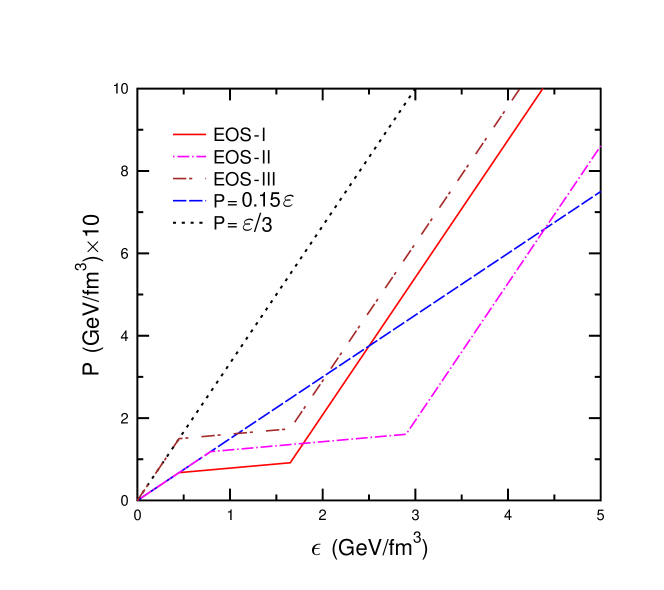
Figure 2: Comparison of different EOSs used in this paper. The lines for EOS–I, EOS–II and EOS–III are calculated using Eqs. (11)–(13) with parameters from Table 1.

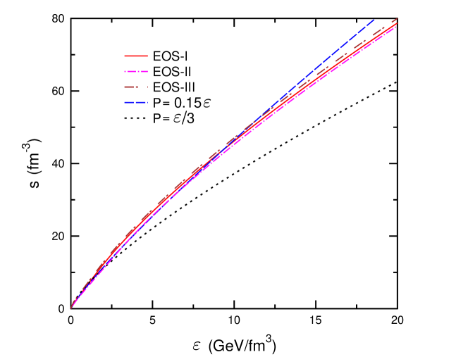
Figure 3: Entropy density as a function of energy density for different EOS s.

The parameters $T_{H}$ and $T_{Q}$ define the boundaries of a mixed phase region separating the hadronic and quark–gluon phases. The critical temperature $T_{c}$ as defined by lattice calculations should lie between $T_{H}$ and $T_{Q}$ , i.e. $T_{c}\simeq(T_{H}+T_{Q})/2$ . Earlier lattice calculations (see e.g. Ref. Kar01 ) predicted the values $T_{c}=(170\pm 10)$ MeV for the baryon–free two–flavor QCD matter. However, a noticeably larger value $T_{c}=(192\pm 11)$ MeV has been reported recently in Ref. Che06 . To probe sensitivity to the actual position of the phase transition, we consider the EOS s with different $T_{H}$ and $T_{Q}$  (see Table 1). The EOS–I corresponds to $T_{H}=165$ MeV and the parameters $\epsilon_{H},\,\epsilon_{Q}$ used in the parametrization LH12 of Ref. Tea01  . In the EOS–II we choose $T_{H}=190$ MeV and scale $\epsilon_{H},\,\epsilon_{Q}$ to get the same values of $\epsilon/T^{4}$ as a function of $T/T_{H}$ . The EOS–III differs from the EOS–I by choosing a higher value $c_{H}^{2}=1/3$ . Finally, the parameters $B_{Q},T_{Q}$ are found from the continuity conditions for $P$ and $T$ . As one can see from Fig. 1, the parametrization (11)–(13) of the EOS leads to the cusp in $\epsilon/T^{4}$ at $T=T_{c}$ , typical for bag–like models. The lattice results for $N_{f}=3$ are overestimated by about 30% in the temperature region from $T_{c}$ to $1.3\hskip 1.0ptT_{c}$ . An attempt to remove this discrepancy has been made in Ref. Moh03 . It is also seen that the EOS–III strongly disagrees with the lattice data in the hadronic phase at $T<T_{c}$ .

Unless stated otherwise, these EOS s are used in the calculations presented in this paper. For comparison, we have performed also calculations for several purely hadronic EOS s. In this case we extend Eq. (11) to energy densities $\epsilon>\epsilon_{H}$ with the same $\epsilon_{H},T_{H}$ as in Table 1, but taking different values of $c_{H}^{2}$ from 0.15 to 1/3. In Figs. 2–3 we compare our EOS s with the phase transition and two hadronic EOS s with constant sound velocities $c_{s}=c_{H}$ . According to Figs. 2, the mixed phase region in the EOS–II occupies a larger interval of energy densities, i.e. this EOS has a larger latent heat as compared to the EOS–I and EOS–III. By this reason, the life–time of the mixed phase should be longer for the EOS–II, assuming the same initial state. One can see that the hadronic EOS $P=c_{H}^{2}\epsilon$ with $c_{H}^{2}=0.15$ (the dashed line in Fig. 2) is much softer at high energy densities as compared to the EOS–I and EOS–II. However, according to Fig. 3, the difference between entropy densities predicted by this hadronic EOS and the EOS s with pase transition is rather small at $\epsilon\lesssim 10$ GeV/fm³. Due to these reasons, the rapidity spectra of pions and kaons predicted by our model for soft EOS s, corresponding to $c_{H}^{2}\lesssim 0.2$, are, in general, rather insensitive to the deconfinement phase transition. On the other hand, the EOS of massless particles, $P=\epsilon/3$ , differs significantly from other EOS s shown in Fig. 3. As a consequence, visible differences with purely hadronic calculations appear only for hard EOS s, i.e. for $c_{H}^{2}\gtrsim 1/3$ .

II.4 Total energy and entropy of the fluid

The equations of ideal fluid dynamics (1)–(3) imply that the total baryon number $B$, total 4–momentum $P^{\hskip 1.0pt\mu}$ and entropy $S$ are the same at any hypersurface $\sigma^{\mu}$ lying above the initial hypersurface (in our case $\tau=\tau_{0}$):

$$B=\int d\sigma_{\nu}n\hskip 1.0ptU^{\nu}=\textrm{const}\,,$$ (14)

$$P^{\mu}=\int d\sigma_{\nu}T^{\mu\nu}=\textrm{const}\,,$$ (15)

$$S=\int d\sigma_{\nu}s\hskip 1.0ptU^{\nu}=\textrm{const}\,.$$ (16)

In the case of central collision of identical nuclei, due to symmetry reasons, the total three–momentum is zero in the c.m. frame. Therefore, Eqs. (15) give only one nontrivial constraint, namely, the conservation of the total c.m. energy, $E=P^{0}$ .

Let us consider a cylindrical volume of matter (”fireball”) expanding in the longitudinal direction and choose the hypersurface of constant $\tau$ . The elements of this hypersurface may be written as

$$d\sigma^{\mu}=S_{\perp}(dz,\bm{0},dt)^{\mu}=\tau S_{\perp}d\eta\hskip 1.0pt(\cosh{\eta},\bm{0},\sinh{\eta})^{\mu},$$ (17)

where $S_{\perp}=\pi R^{2}$ is the transverse cross section of the fireball. Substituting (17) into Eqs. (14)–(16) we get the relations

$$B=S_{\perp}\tau\int\limits_{-\infty}^{+\infty}d\eta\,n\cosh{(Y-\eta)}\,,$$ (18)

$$E=S_{\perp}\tau\int\limits_{-\infty}^{+\infty}d\eta\left[\hskip 1.0pt\epsilon\hskip 1.0pt\cosh{Y}\cosh{(\mbox{$Y-\eta$})}+P\sinh{Y}\sinh{(Y-\eta)}\hskip 1.0pt\right],$$ (19)

$$S=S_{\perp}\tau\int\limits_{-\infty}^{+\infty}d\eta\,s\cosh{(Y-\eta)}\,.$$ (20)

for any fixed $\tau\geqslant\tau_{0}$ . One can determine constants in Eqs. (14)–(16) by using Eqs. (18)–(20) for $\tau=\tau_{0}$. In the baryon–free case ($n$ and $B$ are zero), substituting $\tau=\tau_{0},\,Y=\eta$ into (19)–(20) leads to

$$E=2\hskip 1.0ptS_{\perp}\tau_{0}\int\limits_{0}^{\infty}d\eta\,\epsilon(\tau_{0},\eta)\hskip 1.0pt\cosh{\eta}\,,$$ (21)

$$S=2\hskip 1.0ptS_{\perp}\tau_{0}\int\limits_{0}^{\infty}d\eta\,s(\tau_{0},\eta)\,.$$ (22)

Equations (21)–(22) with $E$ and $S$ from (19)–(20) can be considered as two sum rules for the fluid–dynamical quantities. We have checked that our numerical code conserves the total energy and entropy at any hypersurface $\tau={\rm const}$ on the level better than 1% even for $\tau\gtrsim 200$ fm/c.

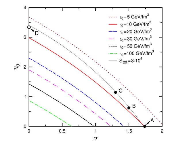
Figure 4: Contours of constant $\epsilon_{0}$ in the $\sigma-\eta_{0}$ plane, corresponding to the fixed total energy (23) of initial fireball in central Au+Au collision ($R=6.5$ fm). Points A–D represent the parameter sets included into the detailed analysis (see below). Point A (D) corresponds to the Gaussian (table–like) initial condition. Thin solid line shows the contour of total entropy $S=3\cdot 10^{4}$ , calculated for the EOS–I.

Below we use Eq. (21) to constrain possible values of the parameters characterizing the initial state. This is possible since the total energy of produced particles can be estimated from experimental data. Indeed, the value of the total energy loss, $\Delta E=73\pm 6$ GeV per participating nucleon, has been obtained from the net baryon rapidity distribution in most central Au+Au collisions Bea04 . This gives an estimate of the total energy of secondaries in the considered reaction:

$$E=N_{\rm part}\hskip 1.0pt\hskip 1.0pt\Delta E\simeq 26.1\,\textrm{TeV}\,,$$ (23)

where $N_{\rm part}\simeq 357$ is the mean number of participating nucleons.

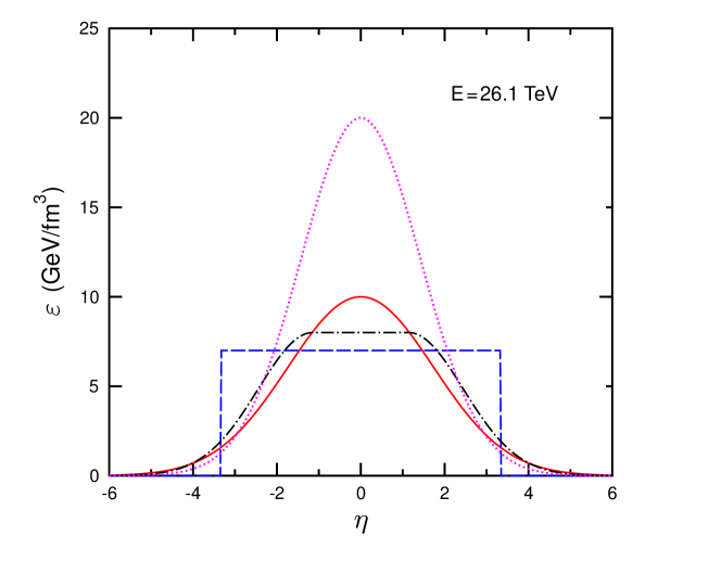
Figure 5: Initial energy density profiles corresponding to the total energy $E=26.1$ TeV in central Au+Au collisions. Solid and dashed–dotted lines correspond, respectively, to the parameter sets A and C (see Table 3). Dashed line is calculated for the table–like profile with $\eta_{0}=3.34$ , $\epsilon_{0}=7$ GeV/fm³ (point D in Fig. 4). Dotted line corresponds to the Gaussian profile with $\sigma=1.42$ , $\epsilon_{0}=20$ GeV/fm³ .

Substituting the parametrization (8) into Eq. (21) and taking the value of $E$ from Eq. (23), one gets the relation between the parameters $\epsilon_{0},\eta_{0},\sigma$. The integration in the r.h.s. of Eq. (19) can be performed analytically. This gives

$$\lambda=\alpha(\sigma)\cosh{\eta_{0}}+\beta(\sigma)\sinh{\eta_{0}}\,.$$ (24)

Here $\lambda=E/(2S_{\perp}\epsilon_{0}\tau_{0})$ and $\alpha,\beta$ are determined as

$$\alpha=\sqrt{\frac{\pi}{2}}\,\sigma\exp{\left(\sigma^{2}/2\right)}\,,~{}~{}~{}\beta=1+\alpha\hskip 1.0pt{\rm erf}\left(\frac{\sigma}{\sqrt{2}}\right).$$ (25)

It is easy to see that the solution of Eq. (24) with respect to $\eta_{0}$ exists at $\alpha<\lambda$ , i.e. at not too large $\sigma$. This solution is given by the expression

$$\eta_{0}=\ln{\left(\frac{\displaystyle\lambda+\sqrt{\lambda^{2}+\beta^{2}-\alpha^{2}}}{\alpha+\beta}\right)}\,.$$ (26)

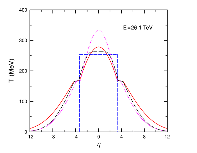
Figure 6: Same as Fig. 5, but for initial temperature profiles. All curves correspond to the EOS–I.

Figure 4 shows contours of constant $\epsilon_{0}$ in the $\eta_{0}-\sigma$ plane. All curves are calculated for the same total energy of the fluid given in Eq. (23). The points at the horizontal (vertical) axis correspond to Gaussian (table–like) initial energy density profiles. One can see that these profiles become narrower for higher maximal energy densities $\epsilon_{0}$ (in this case the contours of equal $\epsilon_{0}$ move closer to the origin of the $\sigma-\eta_{0}$ plane). It is obvious that an additional constraint on the total entropy $S$ would further reduce the freedom in the choice of parameters $\epsilon_{0},\eta_{0},\sigma$ . For example, the best fits of the BRAHMS data (see below) with the EOS–I fall on the line corresponding to $S\simeq 3\cdot 10^{4}$ . According to our analysis, the absolute yields of secondary mesons and antibaryons increase with $S$, even if the total energy is fixed. This effect is well–known from the Landau model Lan53 which postulates that the number of secondaries is proportional to $S$ . The initial temperatures for the considered profiles reach the values 250–350 MeV, well above the critical temperature of the quark–gluon phase transition.

Figure 5 represents some profiles of initial energy density used in this paper. All these profiles correspond to the same total energy of secondaries (23). The corresponding profiles of the initial temperature, $T\hskip 1.0pt(\tau_{0},\eta)$, are shown in Fig. 6. They are calculated by using the EOS–I. Note, that at nonzero $\sigma$ the temperature profiles look much wider as compared to those shown in Fig. 5. One can see that three different phases of matter appear already at the initial state.

II.5 Particle spectra at freeze–out

The momentum spectra of secondary hadrons are calculated by applying the standard Cooper–Frye formula Coo74 , assuming that particles are emitted without further rescatterings from the elements $d\sigma_{\mu}$ of the freeze–out hypersurface $\tau=\tau_{F}(\eta)$ . Then, the invariant momentum distribution for each particle species is given by the expression

$${E}\frac{d^{\hskip 1.0pt3}N}{d^{\hskip 1.0pt3}p}=\frac{d^{\hskip 1.0pt3}N}{dy\hskip 1.0ptd^{\hskip 1.0pt2}p_{T}}=\frac{g}{(2\pi)^{3}}\int d\sigma_{\mu}\hskip 1.0ptp^{\hskip 1.0pt\mu}\left\{\exp\left(\frac{p\hskip 1.0ptU_{F}-\mu_{F}}{T_{F}}\right)\pm 1\right\}^{-1},$$ (27)

where $p^{\hskip 1.0pt\mu}=(E,\bm{p})^{\mu}$ is the 4–momentum of the particle, $y=\tanh^{-1}(p_{z}/E)$ and $\bm{p}_{T}$ are, respectively, its longitudinal rapidity and transverse momentum, $g$ denotes the particle’s statistical weight. The subscript $F$ in the collective 4–velocity $U$ , temperature $T$ and chemical potential $\mu$ implies that these quantities are taken on the freeze–out hypersurface. The plus or minus sign in the r.h.s. of Eq. (27) correspond to fermions or bosons, respectively.

As has been already stated, the effects of transverse expansion are disregarded in our approach. Due to this reason, we cannot describe realistically the $p_{T}$ spectra of produced hadrons, and analyze below only the rapidity spectra. For a cylindrical fireball with transverse cross section $S_{\perp}=\pi R^{2}$ expanding only in the longitudinal direction, one can write $d\sigma^{\mu}=S_{\perp}\hskip 1.0pt(dz_{F},\bm{0},dt_{F})^{\hskip 1.0pt\mu}$ . Using Eq. (4) we get the following relations

$$d\sigma_{\mu}p^{\hskip 1.0pt\mu}=S_{\perp}\hskip 1.0pt(E\hskip 1.0ptdz_{F}-p_{z}\hskip 1.0ptdt_{F})=S_{\perp}\hskip 1.0ptm_{T}\left\{\tau_{F}(\eta)\cosh\hskip 1.0pt(y-\eta)-\tau^{\prime}_{F}(\eta)\sinh\hskip 1.0pt(y-\eta)\right\}d\eta\,.$$ (28)

Here $m_{T}$ is the particle’s transverse mass defined as $m_{T}=\sqrt{m^{2}+\bm{p}_{T}^{\hskip 1.0pt2}}$ , where $m$ is the corresponding vacuum mass. Substituting (28) into (27) and integrating over $\bm{p}_{T}$ we get the expression for the particle rapidity distribution

$$\frac{dN}{dy}=\frac{gS_{\perp}}{4\pi^{2}}\int\limits_{-\infty}^{+\infty}d\eta\left[\tau_{F}(\eta)\cosh\hskip 1.0pt(y-\eta)-\tau^{\prime}_{F}(\eta)\sinh\hskip 1.0pt(y-\eta)\right]\times$$

$$\times\int\limits_{0}^{\infty}dp_{T}p_{T}\hskip 1.0ptm_{T}\left\{\exp\left(\frac{m_{T}\cosh\left[\hskip 1.0pty-Y_{F}(\eta)\right]-\mu_{F}}{T_{F}(\eta)}\right)\pm 1\right\}^{-1},$$ (29)

where $Y_{F}(\eta)$ and $T_{F}(\eta)$ are the flow rapidity and the temperature at $\tau=\tau_{F}(\eta)$ . Note, that the Bjorken model Bjo83 corresponds to $Y_{F}=\eta$ and $\tau_{F},T_{F}$ independent of $\eta$. As can be seen from Eq. (29), the rapidity distributions of all particles should be flat in this case.

II.6 Feeding from resonance decays

In calculating particle spectra one should take into account not only directly produced particles but also feeding from resonance decays. In this paper we explicitly take into account the decays: $\rho\to 2\pi,K^{*}\to K\pi,\overline{\Delta}\to\overline{N}\pi$ , which are most important for describing the spectra of pions, kaons and antiprotons, respectively. The other resonances are taken into account using an approximate procedure explained below. The spectrum of $i$–th particle produced in the two particle decay channel $R\to iX$ is calculated by using the expression Sol90

$$E\frac{d^{\hskip 1.0pt3}N_{R\to i}}{d^{\hskip 1.0pt3}p\hskip 3.0pt}=\frac{d^{\hskip 1.0pt3}N_{R\to i}}{d^{\hskip 1.0pt2}p_{T}dy}=\int\limits_{\displaystyle m_{\rm thr}}^{\infty}d\hskip 1.0ptm_{R}\hskip 1.0ptw\hskip 1.0pt(m_{R})\int d^{\hskip 1.0pt3}p_{R}\hskip 1.0pt\frac{d^{\hskip 1.0pt3}N_{R}}{d^{\hskip 1.0pt3}p_{R}}\cdot\frac{b_{R\to i}}{4\pi q_{0}}\,\delta\left(\frac{p\hskip 1.0ptp_{R}}{m_{R}}-E_{0\hskip 1.0pti}\right),$$ (30)

where the first integration corresponds to averaging over the mass spectrum of the resonance ($m_{\rm thr}=m_{i}+m_{X}$), $p_{R}=(E_{R},\bm{p}_{R})$ and $p=(E,\bm{p})$ are, respectively, the 4–momenta of the resonance $R$ and the particle $i$ . The coefficient $b_{R\to i}$ denotes the branching ratio of the $R\to iX$ decay. The energy and momentum of the i–th particle in the resonance rest frame are determined by the expressions

$$E_{0\hskip 1.0pti}=\sqrt{m_{i}^{2}+q_{0}^{2}}=\frac{m_{R}^{2}+m_{i}^{2}-m_{X}^{2}}{2m_{R}}\,.$$ (31)

The freeze–out momentum spectrum of the resonance, $d^{\hskip 1.0pt3}N_{R}/d^{\hskip 1.0pt3}p_{R}$ , is calculated using Eqs. (27)–(28) with $m=m_{R}$, $g=g_{R}$. Below we assume that the freeze–out temperatures for directly produced particles and corresponding resonances are the same. Calculation of integrals in the r.h.s. of Eq. (30) and the parametrization of $w\hskip 1.0pt(m_{R})$ are discussed in Appendix B.

Table 2: Equilibrium densities of $\pi^{+}$ –, $K^{+}$ –mesons and antiprotons hidden, respectively, in $\rho,K^{*}$ and $\overline{\Delta}$ resonances as well as corresponding enhancement factors at different temperatures $T_{F}$.

$T_{F}$ (MeV)	$d_{\rho}^{\hskip 1.0pt\pi^{+}}n_{\rho}$ (fm-3)	$\alpha_{\rho}^{\hskip 1.0pt\pi^{+}}$	$d_{K^{*}}^{K^{+}}n_{K^{*}}$ (fm-3)	$\alpha_{K^{*}}^{K^{+}}$	$d_{\hskip 1.0pt\overline{\Delta}}^{\hskip 1.0pt\overline{p}}n_{\overline{\Delta}}$ (fm-3)	$\alpha_{\hskip 1.0pt\overline{\Delta}}^{\hskip 1.0pt\overline{p}}$
100	$5.74\cdot 10^{-4}$	2.30	$1.08\cdot 10^{-4}$	1.21	$1.48\cdot 10^{-5}$	1.09
110	$1.37\cdot 10^{-3}$	2.28	$2.85\cdot 10^{-4}$	1.26	$5.30\cdot 10^{-5}$	1.12
120	$2.87\cdot 10^{-3}$	2.31	$6.50\cdot 10^{-4}$	1.30	$1.56\cdot 10^{-4}$	1.15
130	$5.43\cdot 10^{-3}$	2.37	$1.32\cdot 10^{-3}$	1.35	$3.92\cdot 10^{-4}$	1.18
140	$9.48\cdot 10^{-3}$	2.46	$2.46\cdot 10^{-3}$	1.40	$8.74\cdot 10^{-4}$	1.21
150	$1.55\cdot 10^{-2}$	2.57	$4.24\cdot 10^{-3}$	1.46	$1.77\cdot 10^{-3}$	1.24
160	$2.41\cdot 10^{-2}$	2.70	$6.90\cdot 10^{-3}$	1.51	$3.29\cdot 10^{-3}$	1.28
165	$2.95\cdot 10^{-2}$	2.77	$8.63\cdot 10^{-3}$	1.54	$4.39\cdot 10^{-3}$	1.29
170	$3.58\cdot 10^{-2}$	2.83	$1.07\cdot 10^{-2}$	1.57	$5.75\cdot 10^{-3}$	1.31
180	$5.13\cdot 10^{-2}$	2.98	$1.58\cdot 10^{-2}$	1.62	$9.50\cdot 10^{-3}$	1.34
190	$7.11\cdot 10^{-2}$	3.13	$2.27\cdot 10^{-2}$	1.68	$1.50\cdot 10^{-2}$	1.37

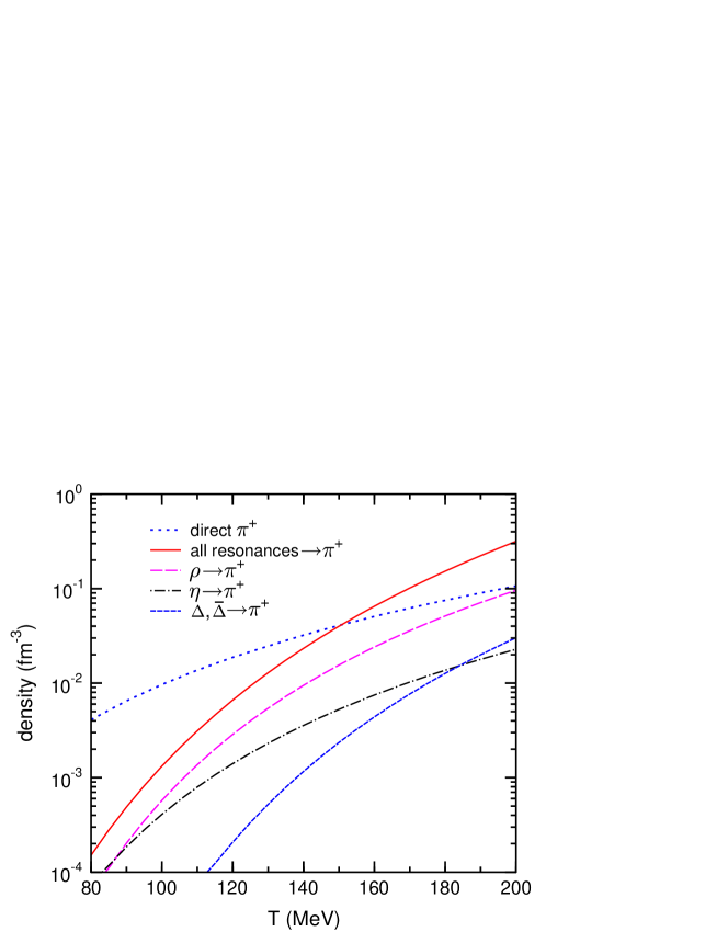
Figure 7: Equilibrium densities of $\pi^{+}$ mesons hidden in resonances $\eta,\rho,\Delta,\overline{\Delta}$ as functions of temperature $T$ . Solid line shows sum over all mesonic and baryonic resonances (see text). Dotted line represents the equilibrium density of free $\pi^{+}$–mesons (not hidden in resonances).

The detailed calculations in this paper are made for spectra of charged pions ($i=\pi^{+}$), kaons ($i=K^{+}$) and antiprotons ($i=\overline{p}$). In these cases the most important contributions are given by decays of resonances $R=R_{0}=\rho,\,K^{*}(892),\,\overline{\Delta}\hskip 1.0pt(1232)$ , respectively. To take into account other hadronic resonances ($R\neq R_{0}$) we assume that the contribution of the resonance $R$ is proportional to its equilibrium density, $n_{R}\hskip 1.0pt(T_{F})$ multiplied by $d_{R}^{\,i}$, the average number of i–th particles produced in $R\to iX$ decays (e.g. $d_{\rho}^{\,i}=2/3,\mbox{$d_{\eta}^{\,i}=0.65$}\ldots$  for $i=\pi^{+}$). Within this approximation one has

$$\sum\limits_{R}\frac{\displaystyle d^{\hskip 1.0pt3}N_{R\to i}}{\displaystyle dy\hskip 1.0ptd^{\hskip 1.0pt2}p_{T}}=\alpha_{R_{0}}^{i}\hskip 1.0pt\frac{\displaystyle d^{\hskip 1.0pt3}N_{R_{0}\to i}}{\displaystyle dy\hskip 1.0ptd^{\hskip 1.0pt2}p_{T}}\,,$$ (32)

where the enhancement factor $\alpha_{R_{0}}^{i}$ is

$$\alpha_{R_{0}}^{i}=\sum\limits_{R}\frac{d_{R}^{\hskip 1.0pti}}{d_{R_{0}}^{\,i}}\frac{n_{R}\hskip 1.0pt(T_{F})}{n_{R_{0}}(T_{F})}\,.$$ (33)

Here $n_{R}$ is the total density of resonances $R$ at the temperature $T$ summed over all isospin states of $R$ . For simplicity, we calculate $n_{R}$ in the zero width approximation. More details of $n_{R}$ and $d_{R}^{\,i}$ calculations can be found in Ref. Beb92 . We have checked for several resonances with two–body decays (e.g. for $i=\pi$ and $R=K^{*}$) that such a procedure yields a very good accuracy. We include meson (baryon and antibaryon) resonances with masses up to 1.3 (1.65) GeV and widths $\Gamma<150$ MeV. The statistical weights, masses and branching ratios of these resonances are taken from Ref. PDG04  . The results for different $T_{F}$ are shown in Table 2. One can see that factors $\alpha_{R}^{i}$ significantly exceed unity (especially for pions) and increase with temperature.

Figure 7 shows the temperature dependence of $\pi^{+}$–meson densities, $d_{R}^{\hskip 1.0pt\pi^{+}}n_{R}$, hidden in different resonances $R$ . One can see that, compared to other resonance decays, the channels $\rho\to 2\pi$ give the largest contribution at all temperatures. According to this calculation, in equilibrium hadronic matter the fraction of ”free” pions (not hidden in resonances) is smaller than 50% at temperatures $T\gtrsim 150$ MeV.

III Results

III.1 Dynamical evolution of matter

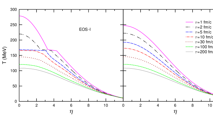
Figure 8: Temperature profiles at different proper times $\tau$ calculated for initial conditions corresponding to the parameter set A. Only the forward hemisphere ($\eta\geqslant 0$) is shown. Left and right panels correspond, respectively, to the EOS–I and the hadronic EOS $P=c_{H}^{2}\hskip 1.0pt\epsilon$  with $c_{H}^{2}=0.15$ .

Space–time evolution of matter as predicted by the present model is illustrated in Figs. 8–13. In particular, Figs. 8–9 show profiles of the temperature and the collective rapidity at different proper times $\tau$ . Here we consider the Gaussian–like initial conditions, with parameters from the set A (see Fig. 4 and Table 3). For comparison, the results are presented for the EOS–I and for the hadronic EOS with $c_{s}^{2}=0.15$. One can see that in the case of the phase transition the model predicts appearance of a a flat shoulder in $T\hskip 1.0pt(\eta)$ and local minima in $Y\hskip 1.0pt(\eta)$ which are clearly visible at $\tau\lesssim 10$ fm/c. This is a manifestation of the mixed phase which exists during the time interval $\Delta\tau\sim 10$ fm/c. According to Fig. 8, the largest volume of this phase in the $\eta$–space takes place at $\tau\sim 5$ fm/c. In the considered case the ”memory” of the quark phase is practically washed out at $\tau\gtrsim 30$ fm/c. As one can see from Fig. 9, at such late times deviation from the Bjorken scaling ($Y=\eta$) does not exceed 5%.

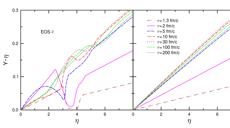
Figure 9: Same as Fig. 8, but for collective rapidity profiles.

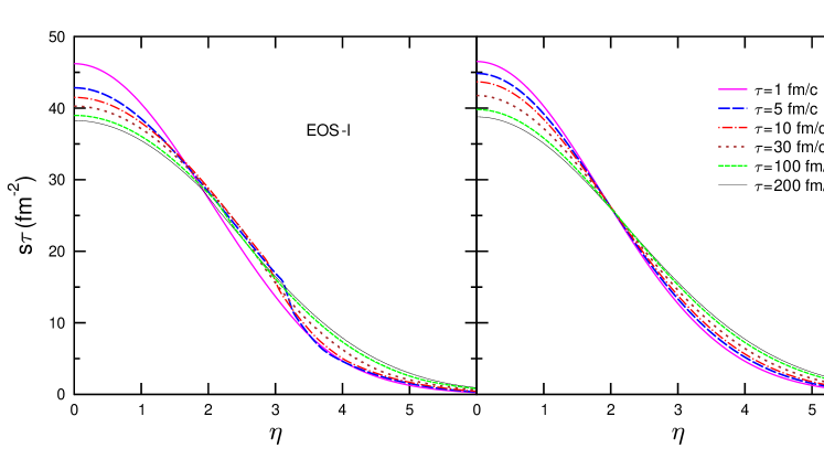
Figure 10: Same as Fig. 8, but for profiles of entropy density multiplied by $\tau$ .

Another important quantity which shows deviation from scaling hydrodynamics is the entropy density $s$ multiplied by $\tau$. As noted in footnote to Eqs. (9), $s\tau$ is constant in the Bjorken model. In Fig. 10 we show profiles of $s\tau$ at different $\tau\geqslant\tau_{0}$ , again for the parameter set A. Two conclusions can be made here. First, these profiles are only weakly sensitive to the presence of the phase transition. We have already noted this when discussing Fig. 3. Second, one can clearly see that $s\tau\neq\textrm{const}$ as a function of $\tau$ . In contrast to the Bjorken model, $s\tau$ drops by about 15% for $|\eta|<1$ at $\tau\gtrsim 20$ fm/c. Due to this reason, we think that the above–mentioned 2+1 dimensional models Kol99 ; Bas00 ; Per00 ; Kol01 ; Tea01 , which assume Bjorken scaling in the beam direction, are not very accurate even for the slice around $\eta=0$.

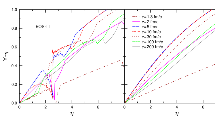
Figure 11: Collective rapidity profiles at different proper times $\tau$ calculated for initial conditions with parameters $\epsilon_{0}=50$ GeV/fm${}^{3},\,\eta_{0}=0,\,\sigma=0.98$ . Left and right panel correspond, respectively, to the EOS–III and the hadronic EOS $P=\epsilon/3$ .

To study sensitivity of flow to the EOS of the hadronic phase, we have performed calculations for different sound velocities $c_{H}$ keeping other parameters of the EOS the same as in Figs. 8–10. It is found that at fixed total energy $E$ , acceleration of the fluid is stronger for harder EOS s characterized by larger $c_{H}$ . Figure 11 shows profiles of flow rapidity for the EOS s with $c_{H}^{2}=1/3$. Comparison with Fig. 9 shows that the transition from $c_{H}^{2}=0.15$ to $c_{H}^{2}=1/3$ results in about 3–fold increase of relative flow rapidity $Y-\eta$  (this quantity characterizes deviations from the inertial expansion of matter). Comparison of the left and right panels in Fig. 11 reveals that the sensitivity of flow to the phase transition is much stronger as compared with the soft EOS considered above ($c_{H}^{2}=0.15$). The differences in acceleration at late times of 30–50 fm/c are especially visible for $|\eta|\lesssim 2$ . Qualitative explanation of this effect is obvious: fluid elements at such $\eta$ exhibit smaller acceleration in the case of phase transition. This is a manifestation of the mixed phase which is characterized by small gradients of pressure.

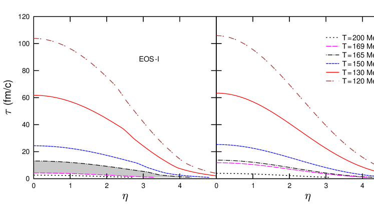
Figure 12: Isotherms in the $\eta-\tau$ plane calculated for the parameter set A. Left and right panels correspond to the same EOS s as in Fig. 8. Shaded region indicates the mixed phase.

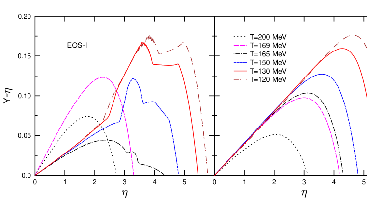
Figure 13: Same as Fig. 12, but for profiles of collective rapidity corresponding to fixed temperatures.

Figure 12 shows the fluid isotherms in the $\eta-\tau$ plane. The profiles of flow rapidity at hypersurfaces of constant temperature are shown in Fig.  13. This information is used to calculate particle momentum distributions by using formulae of Sect. II.5. According to Fig. 12 (see the left panel), the initial stage of the evolution when matter is in the quark–gluon phase, lasts only for a very short time, of about 5 fm/c. The region of the mixed phase is crossed in less than 10 fm/c. This clearly shows that the slowing down of expansion associated with the ”soft point” of the EOS plays no role, when the initial state lies much higher in the energy density than the phase transition region. In this situation the system spends the longest time in the hadronic phase. The freeze-out at $T_{F}=130$ MeV requires an expansion time of about 60 fm/c at $\eta=0$. This is certainly a very long time which is seemingly in contradiction with some experimental findings. Indeed, the interferometric measurements Adl01 show much shorter times of hadron emission, of the order of 10 fm/c. As follows from our results, this discrepancy can not be removed by considering other EOS or initial conditions. A considerable reduction of the freeze–out times can be achieved by including the effects of transverse expansion and chemical nonequilibrium Hir02 . However, this will not change essentially the dynamics of the early stage ($\tau\lesssim 10$ fm/c) when expansion is predominantly one–dimensional. A more radical solution would be an explosive decomposition of the quark–gluon plasma, proposed in Ref. Mis99 . This may happen at very early times, right after crossing the critical temperature line, when the plasma pressure becomes very small or negative. We shall consider this possibility in a forthcoming publication.

III.2 Rapidity spectra of secondary hadrons

Below we show the results for rapidity distributions of $\pi$– and $K$–mesons as well as antiprotons produced in central Au+Au collisions at $\sqrt{s_{\scriptscriptstyle NN}}=200$ GeV. These results are compared with data of the BRAHMS Collaboration Bea04 ; Bea05 for most central (0%–5%) collisions.

Table 3: Parameters of the initial states which give the best fits of the pion, kaon and antiproton rapidity spectra observed in central Au+Au collisions at $\sqrt{s_{\scriptscriptstyle NN}}=200$ GeV. All sets correspond to the EOS–I. $T_{0}$ denotes the maximum temperature at $\tau=\tau_{0}$ . $E_{1}$ and $E_{3}$ are total energies of produced particles within the rapidity intervals $|y|<1$ and $|y|<3$, respectively.

set	$\epsilon_{0}$ (GeV/fm3)	$\sigma$	$\eta_{0}$	$T_{0}$ (MeV)	$E_{1}$ (TeV)	$E_{3}$ (TeV)	$E/S$ (GeV)
A	10	1.74	0	279	1.53	9.25	0.89
B	9	1.50	0.62	271	1.54	9.59	0.86
C	8	1.30	1.14	263	1.49	9.55	0.86

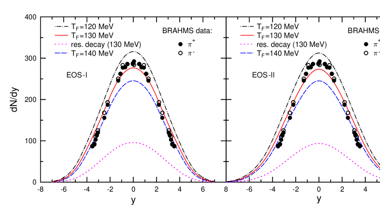
Figure 14: Rapidity distribution of $\pi^{+}$–mesons in central Au+Au collisions at $\sqrt{s_{\scriptscriptstyle NN}}=200$ GeV. Left panel shows results of hydrodynamical calculations for the EOS–I and initial conditions with parameters $\epsilon_{0}=10$ GeV/fm³, $\eta_{0}=0$, $\sigma=1.74$ (set A in Table 3). Right panel corresponds to the EOS–II and the parameters $\epsilon_{0}=5$ GeV/fm³, $\eta_{0}=0$, $\sigma=2.02$. Solid, dashed and dashed–dotted curves correspond to different values of the freeze–out temperature $T_{F}$ . The dotted line shows contribution of resonance decays in the case $T_{F}=130$ MeV. Experimental data are taken from Ref. Bea05 .

We have considered different profiles of the initial energy density, ranging from the Gaussian–like ($\eta_{0}=0$) to the table–like ($\sigma=0$) initial states. We found that in the case of EOS–I it is not possible to reproduce the BRAHMS data on the pion and kaon rapidity spectra in Au+Au collisions by choosing either too small ($\epsilon_{0}\lesssim 5$ GeV/fm³) or too large ($\epsilon_{0}\gtrsim 15$ GeV/fm³) initial energy densities. For such $\epsilon_{0}$ values the pion and kaon yields can not be reproduced with any $T_{F}$ . According to our calculations, the quality of fits is noticeably reduced for initial energy density profiles with sharp edges, corresponding to $\sigma<1$ . As follows from the constraint (23), such profiles should have a very large $\epsilon_{0}$ or a significant plateau $-\eta_{0}<\eta<\eta_{0}$. This would lead to more flat rapidity distributions of pions and kaons as compared to the BRAHMS data (see the next section).

A few parameter sets which lead to good fits with the EOS–I are listed in Table 3. In these calculations we choose various $\epsilon_{0}$ and $\sigma$ and determine $\eta_{0}$ from the total energy constraint (23).

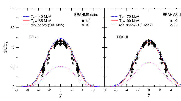
Figure 15: Same as Fig. 14, but for $K^{+}$–meson rapidity distributions.

It is interesting that the initial states A–C have approximately the same total entropy $S\simeq 3\cdot 10^{4}$ (see Fig. 4). This is not surprising because the total entropy should be proportional to the total multiplicity of secondary mesons which is approximately same for all good fits. As one can see from the last column of Table 3, the corresponding $E/S$–ratios fall into a narrow interval $0.86-0.89$ GeV. This observation is similar to the result of Ref. Cle98 that the observed ratio of the rest–frame energy to the multiplicity of produced hadrons is constant as a function of the bombarding energy.

To check the sensitivity to the parameters of the phase transition, we have also calculated the pion and kaon rapidity distributions for the EOS–II. It is found that with the same initial energy profiles as for the EOS–I, it is not possible to reproduce the observed spectra at any freeze–out temperature. In particular, the predicted kaon yield is strongly overestimated  at $100\,\textrm{MeV}<T_{F}<T_{H}=190$ MeV. Nevertheless, the BRAHMS data can be well reproduced with the EOS–II too, when taking smaller initial energy densities as compared with the EOS–I. Fits of approximately same quality are obtained for $\epsilon_{0}\simeq 5$ GeV/fm³ . As before, in choosing the initial conditions we apply the constraint (23) for the total energy of produced particles. Similarly to the case of the EOS–I, the data are better reproduced for initial profiles with small $\eta_{0}\lesssim 1$ .

Figures 14–15 show the model results for pion and kaon rapidity distributions obtained for the EOS–I and EOS–II. These results correspond to Gaussian initial profiles with $\eta_{0}=0$ . For both EOS s we choose the parameter $\epsilon_{0}$ to obtain the best fit of the BRAHMS data. Although the overall fits are very similar for both EOS s, the rapidity spectra obtained with the EOS–II are slightly broader than those with the EOS–I. In the same figures we demonstrate sensitivity to the choice of the freeze–out temperature. The best fits of the pion spectrum are achieved with $T_{F}\simeq 130$ MeV (see Fig. 14). On the other hand, the kaon spectrum can be well reproduced only by assuming that kaons decouple at the very beginning of the hadronic stage, i.e. at $T_{F}\simeq T_{H}=165\,(190)$ MeV for EOS–I (II). The contribution of resonance decays turns out to be rather significant, especially in the central rapidity region, where it amounts to about 35% (45%) of the total pion (kaon) yield.

Figure 16: Rapidity distribution of $\pi^{+}$–mesons in central Au+Au collisions at $\sqrt{s_{\scriptscriptstyle NN}}=200$ GeV calculated for initial conditions with parameters $\epsilon_{0}=50$ GeV/fm³, $\eta_{0}=0$, $\sigma=0.96$. The solid line corresponds to the EOS–III. The dashed line is calculated for the hadronic EOS $P=\epsilon/3$ . Experimental data are taken from Ref. Bea05 .

According to Fig. 14, larger yields of secondary pions are predicted for smaller freeze–out temperatures. A much weaker sensitivity to $T_{F}$ is found for kaons (see Fig. 15). This difference can be explained by the large difference between the pion and kaon masses. Indeed, in the case of direct pions, a good approximation at $T_{F}>100$ MeV is to replace the transverse mass $m_{T}$ in Eq. (29) by the pion transverse momentum $p_{T}$. Neglecting the term with $\tau^{\hskip 1.0pt\prime}_{F}$ in the r.h.s. of this equation, one can show that the rapidity distribution of pions at $y=0$ is proportional to $\xi=\tau_{F}(\eta)\hskip 1.0pt\cosh{\eta}\cdot T_{F}^{\hskip 1.0pt3}/\cosh^{3}{Y_{F}(\eta)}$ integrated over all $\eta$ . For a rough estimate, one can use the Bjorken relations Bjo83 $\mbox{$Y_{F}=\eta$},\,s_{F}\tau_{F}=s_{0}\tau_{0}$ , where $s_{F}$ is the entropy density at $T=T_{F}$ . Using Eq. (11) one gets $\tau_{F}\propto s_{F}^{-1}\propto T_{F}^{-1/c_{H}^{2}}$ and therefore, $\xi\propto T_{F}^{3-1/c_{H}^{2}}$. This shows that for $c_{H}^{2}<1/3$ the pion yield grows with decreasing $T_{F}$. Qualitatively, one can say that at low enough $c_{H}$ the increase of the spatial volume at freeze–out compensates for the decrease of the pion occupation numbers at smaller $T_{F}$. This effect is somewhat reduced because of a decreasing resonance contribution at smaller temperatures. It is obvious that for kaons this effect should be much weaker due to the presence of the activation exponent $\exp{(-m_{K}/T_{F})}$ . In fact, a numerical calculation for the same EOS and initial state shows that the kaon yield changes nonmonotonically: first it slightly increases when temperature goes down but then it starts to decrease at lower $T_{F}$ .

Figure 17: Same as Fig. 16, but for $K^{+}$–meson rapidity distributions.

To investigate sensitivity of particle spectra to the presence of the phase transition, we have performed calculations with purely hadronic EOS s. In this case we use the same initial conditions as before, but apply Eq. (11) for all stages of the reaction, including the high density phase. Our analysis shows that for soft hadronic EOS with $c_{H}^{2}\lesssim 0.2$ it is possible to reproduce the observed pion and kaon data with approximately the same fit quality as in the calculations with the quark–gluon phase transition. Furthermore, the corresponding freeze–out temperatures do not change significantly. However, we could not achieve satisfactory fits for the ”hard” hadronic EOS with $c_{H}^{2}\geqslant 1/3$. Figures 16–17 show particle spectra calculated for the same EOS s and initial conditions as in Fig. 11. One can see that the hadronic EOS with $c_{H}^{2}=1/3$ leads to too wide rapidity distributions for both pions and kaons. The reason is that the higher pressure in the hadronic EOS gives a stronger push to the matter in forward and backward directions. From these findings we conclude that a certain degree of softening of the EOS is required to reproduce the pion and kaon rapidity distributions. Our analysis shows that reasonable fits of data for EOS s with $c_{H}\gtrsim 0.2$  (with and without the phase transition) can be achieved only when freeze–out temperatures for kaons are smaller than for pions. We find this situation unphysical, because kaons have smaller rescattering cross sections and, therefore, there is no reason for delayed kaon emission.

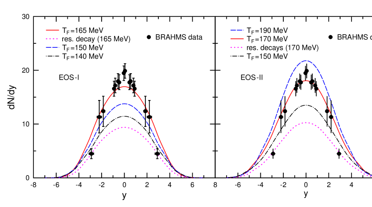
Figure 18: Same as Fig. 14, but for antiproton rapidity distributions. All results are obtained assuming $\mu_{F}=0$. Experimental data are taken from Ref. Bea04 .

It turned out that using the parameter sets from Table 3, one can also reproduce reasonably well the antiproton rapidity spectra measured by the BRAHMS Collaboration Bea04 . Figure 18 shows the antiproton rapidity distributions, calculated for the parameter set A. In this case we explicitly take into account the contribution of the $\overline{\Delta}(1232)\to\pi\overline{p}$ decays, ignoring the width of $\Delta$–isobar. Contributions of higher antibaryon resonances are taken into account in a similar way as for pions and kaons. The resonance contribution reaches about 55% at $T_{F}=165$ MeV. One should consider these results as an upper bound for the antiproton yield. A more realistic model should include the effect of nonzero baryon chemical potentials which will certainly reduce the antibaryon yield. The thermal model analysis of RHIC data, performed in Refs. And04 ; And06 , gives rather low values for the baryon chemical potentials, $\mu_{F}\sim 30$ MeV, at midrapidity. This will suppress the antiproton yield by a factor $\sim\exp{(-\mu_{F}/T_{F})}\sim 0.8$ .

III.3 Rapidity distribution of total energy

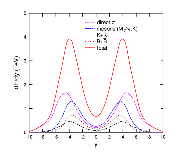
Figure 19: Rapidity distribution of the total energy of secondary hadrons in central Au+Au collisions at $\sqrt{s_{\scriptscriptstyle NN}}=200$ GeV. Shown are results for the EOS–I and parameter set A.

In order to check the energy balance in the considered reaction, we have calculated additionally the rapidity distribution of the total energy of secondary particles, $dE/dy$ . In the zero–width approximation this quantity can be written as

$$\frac{dE}{dy}=\cosh{y}\sum\limits_{i}\int d^{\hskip 1.0pt2}p_{T}\frac{d^{3}N_{i}}{d^{\hskip 1.0pt2}p_{T}dy}\sqrt{m_{i}^{2}+p_{T}^{\,2}}\,,$$ (34)

where the sum goes over all hadronic species. In calculating $dE/dy$ we take into account not only direct pions ($i=\pi$) and kaons ($i=K,\overline{K}$), but also 14 lowest mass mesons with widths $\Gamma\lesssim 150$ MeV PDG04 :

$$M=\eta,\rho,\omega,\eta^{\,\prime},f_{0},a_{0},\phi,b_{1},f_{1},a_{2},\eta\hskip 1.0pt(1295),K^{*},K_{1},K^{*}_{2}\,.$$ (35)

We also include 12 strange and nonstrange baryon–antibaryon ($B\overline{B}$) species:

$$B=N,N(1520),N(1535),\Delta,\Delta(1520),\Delta(1620),\Lambda,\Lambda(1405),\Lambda(1520),\Sigma,\Sigma(1385),\Xi\,.$$ (36)

In calculating contributions of different species to $dE/dy$ in the r.h.s. of Eq. (34) we use the freeze–out temperatures obtained by fitting the pion ($T_{F}^{\pi}$), kaon ($T_{F}^{K}$) and antiproton ($T_{F}^{\overline{p}}$) rapidity distributions. We choose these temperatures to find, respectively, the contributions of free pions ($i=\pi$), heavy mesons ($i=M$ , where $M\neq\pi$) and baryon–antibaryon pairs ($i=B,\overline{B}$). In particular, the results shown in Fig. 19 correspond to $T_{F}^{\pi}=130$ MeV, $T_{F}^{K}=T_{F}^{\overline{p}}=165$ MeV. By integrating $dE/dy$, we have determined $E_{1}$ and $E_{3}$, the total energies of secondaries within the rapidity intervals $|y|<1$ and $|y|<3$, respectively. The BRAHMS Collaboration estimated $E_{1,3}$ from the rapidity distributions of charged pions, kaons, protons and antiprotons in most central Au+Au collisions at $\sqrt{s_{\scriptscriptstyle NN}}=200$ GeV. The values $E_{1}\simeq 1.5\,\textrm{TeV},\hskip 8.61108pt\mbox{$E_{3}\simeq 9\,\textrm{TeV}$}$ have been reported in Ref. Ars05 . From Table 3 one can see that these values are well reproduced by the model.

Based on the above analysis we conclude that within the hydrodynamical model the BRAHMS data can be well described with the EOS-I and EOS–II and the parameters of the initial state ($\tau_{0}=1$ fm/c) $\sigma\simeq 1.5-2,~{}~{}\eta_{0}\lesssim 1$ . The maximal initial energy density, $\epsilon_{0}$, is sensitive to the critical temperature of the phase transition. For the EOS–I ($T_{c}\simeq 167$ MeV) we get the estimate $\epsilon_{0}\simeq 9\pm 1$ GeV/fm³ while for the EOS–II ($T_{c}\simeq 192$ MeV) the required values of $\epsilon_{0}$ are lower by about a factor of two.

III.4 Comparison of Landau–like and Bjorken–like initial conditions

As discussed above, the initial profiles which give the best fits of particle rapidity distributions are intermediate between the Landau and Bjorken limits. Nevertheless it is interesting to compare the model predictions for the Landau–like and Bjorken–like initial states. In fact, the Landau initial conditions correspond to points situated near the origin of the $\sigma-\eta_{0}$ plane in Fig. 4. On the other hand, the Bjorken–like states correspond to table–like states with small $\sigma$ and large $\eta_{0}$ i.e. to points near the vertical axis in Fig. 4 , away from the origin.

Let us first consider the limiting case of the Landau model.

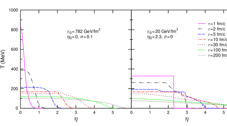
Figure 20: Temperature profiles at different proper times $\tau$ calculated for the EOS–III. Left (right) panel corresponds to the Gaussian (table-like) initial conditions with parameters given in the figures.

In its simplest version, for the EOS s with $c_{s}={\rm const}$, this model predicts a Gaussian rapidity distribution of secondary pions. Originally, the Landau model was formulated for proton–proton collisions. Below we assume that pion rapidity distributions in $pp$–reactions and central collisions of equal nuclei have the same shapes at the same c.m. energy $\sqrt{s_{\scriptscriptstyle NN}}$. Then the following approximate formulae can be derived Shu72

$$\frac{dN_{\pi}}{dy}=C_{\pi}\frac{s_{\scriptscriptstyle NN}^{\,\alpha}}{\sigma_{\rm Lan}}\exp{\left[-\frac{y^{2}}{~{}~{}2\hskip 1.0pt\sigma_{\rm Lan}^{2}}\right]},$$ (37)

where the normalization constant $C_{\pi}$ does not depend on the bombarding energy and

$$\alpha=\frac{1-c_{s}^{2}}{2\hskip 1.0pt(1+c_{s}^{2})}\,,~{}~{}\sigma_{\rm Lan}^{2}\simeq\frac{8}{3}\frac{\displaystyle c_{s}^{2}}{\displaystyle 1-c_{s}^{4}}\ln{\frac{\sqrt{s_{\scriptscriptstyle NN}}}{2\hskip 1.0ptm_{N}}}\,.$$ (38)

For $c_{s}^{2}=1/3$ and $\sqrt{s_{\scriptscriptstyle NN}}=200$ GeV one obtains $\alpha=1/4$ and $\sigma_{\rm Lan}\simeq 2.16$ , the values often quoted in the literature Bea05 ; Ble05 . On the other hand, for $c_{s}^{2}=0.15$ , which is preferable from the viewpoint of our previous analysis (see Sect. III.2), the predicted width is only 1.38 i.e. significantly smaller than observed by the BRAHMS Collaboration. Note, that the analytical formulae (37)–(38) are obtained for the case of constant sound velocity and can not be applied for EOSs with a first–order pase transition. In this connection we think that attempts Ble05 to extract a unique sound velocity from pion spectra observed at a specific bombarding energy are unjustified.

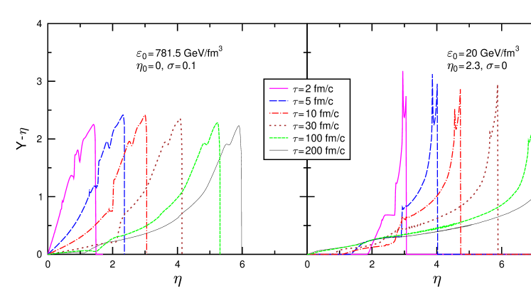
Figure 21: Same as Fig. 20, but for collective rapidity profiles.

Within the Landau model one assumes that a thin disk–like fireball is created at some time $t=t_{0}$ after beginning of the nuclear collision . It is postulated that this fireball is initially at rest ($Y=0$) in the c.m. frame. It has the transverse cross section $S_{\perp}=\pi R^{2}$ and the longitudinal size $\Delta z\sim 2R/\gamma$ . Here $R$ is the geometrical radius of colliding nuclei, $\gamma\sim\sqrt{s_{\scriptscriptstyle NN}}/2m_{N}$ is the c.m. Lorentz–factor. The total energy, $E$ , is normally assumed to be $E=\kappa\hskip 1.0pt(\gamma-1)\hskip 1.0ptN_{\rm part}m_{N}$ where $N_{\rm part}$ is the number of participating nucleons and $\kappa\sim 0.5-0.7$ is the so–called inelasticity coefficient. At the c.m. energy $\sqrt{s_{\scriptscriptstyle NN}}=200$ GeV the Lorentz–factor $\gamma\sim 100$ and, therefore, $\Delta z\lesssim 0.1$ fm. If $t_{0}$ is not too small, the initial fireball occupies a region of small space–time rapidities, $|\eta|<\Delta\eta\simeq\Delta z/t_{0}$, and one can approximately apply the parametrization of initial state (8) with $\eta_{0}=0$ and $\sigma\sim 2R/(\gamma t_{0})$. Note, that at small $|\eta|$ the difference between the initial flow profiles $Y=\eta$ and $Y=0$ is negligible. Using further Eq. (24), one can estimate the maximal energy density of the fireball as $\epsilon_{0}\sim E\,(\sqrt{2\pi^{3}}R^{2}\sigma t_{0})^{-1}$ . On the basis of these arguments we conclude that the Landau model can be approximately simulated within our approach by taking the Gaussian initial profile with small $\sigma\propto\gamma^{-1}$ and large $\epsilon_{0}\propto\gamma^{2}$ .

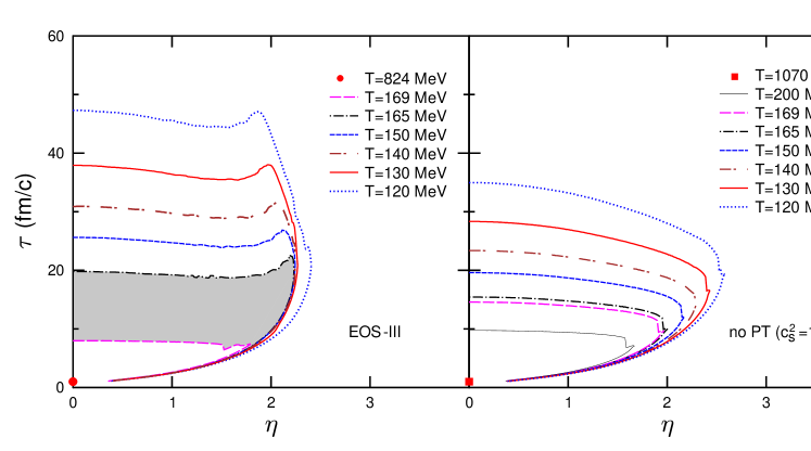
Figure 22: Isotherms in the $\eta-\tau$ plane calculated for the initial parameters $\epsilon_{0}=782$  GeV/fm³, $\eta_{0}=0$ , $\sigma=0.1$. Left panel corresponds to the EOS–III. Right panel shows results for the hadronic EOS $P=\epsilon/3$. Shaded region indicates the mixed phase. Dots near the origin correspond to the maximal initial temperature.

For illustration, in this section we present the numerical results for the parameters of the initial state $\eta_{0}=0,\,\sigma=0.1$ and $t_{0}\simeq\tau_{0}=1$ fm/c. Again, the total energy is fixed at the value (23). This gives the estimate $\epsilon_{0}\simeq 782$ GeV/fm³ . Figures 20–21 show profiles of the temperature and flow rapidity at different proper times $\tau\geqslant\tau_{0}$ . For comparison with the Bjorken–like scenario, we also present results for a ”broad”, table–like initial state with $\sigma=0,\,\eta_{0}=2.3,\,\epsilon_{0}=20$ GeV/fm³ (this state has the same total energy and entropy). The difference between the fluid dynamics predicted for the Landau–like and Bjorken–like initial states is clearly visible at $\tau\lesssim 10$ fm/c and $|\eta|\gtrsim 2$ . It is interesting that asymptotically, for $\tau\gtrsim 100$ fm/c, the ”Landau” profiles at $|\eta|\lesssim 2$ behave similar to Bjorken’s scaling solution, $Y\simeq\eta,\,T\simeq\textrm{const}$ . On the other hand, the two solutions differ significantly at large $\eta$ , where the Bjorken–like initial state leas to a very strong acceleration of the fluid near its outer edge.

Figure 22 shows contours of constant temperature for the Landau–like initial state. These contours are calculated for two EOS s, with and without the phase transition. Contrary to the case of a broader initial energy density profile presented in Fig. 12, now the contours have a ”pocket–like” structure with back–bending portions of isotherms. One can see a moderate sensitivity of isotherms to the presence of a phase transition. As discussed in Sect.  III.1, this sensitivity becomes even weaker for softer EOS s.

Now we present the rapidity distributions of pions and kaons calculated with the Landau–like initial conditions for several EOS s. Our analysis shows that it is not possible to reproduce the pion spectra with EOS–I and EOS–II. The corresponding pion yields are too high at any $T_{F}<T_{H}$ . Both the pion and kaon yields become acceptable only for EOS s with $c_{H}^{2}\gtrsim 0.2$ . This is demonstrated in Figs. 23–24 which show the pion and kaon spectra for two EOS s with $c_{H}^{2}=1/5$ and 1/3. The first EOS corresponds to the EOS–I, but with $c_{H}^{2}=0.2$ (this is in fact the EOS LH12 from Ref. Tea01 ). In Fig. 23 one can see that the pion spectrum calculated with this EOS is somewhat broader as compared with the experimental data. On the other hand, Fig. 24 shows that for the EOS–III ($c_{H}^{2}=1/3$) the predicted kaon spectrum is noticeably broader than observed experimentally. Therefore, we conclude that the BRAHMS data disfavor the Landau–like initial conditions at RHIC bombarding energies.

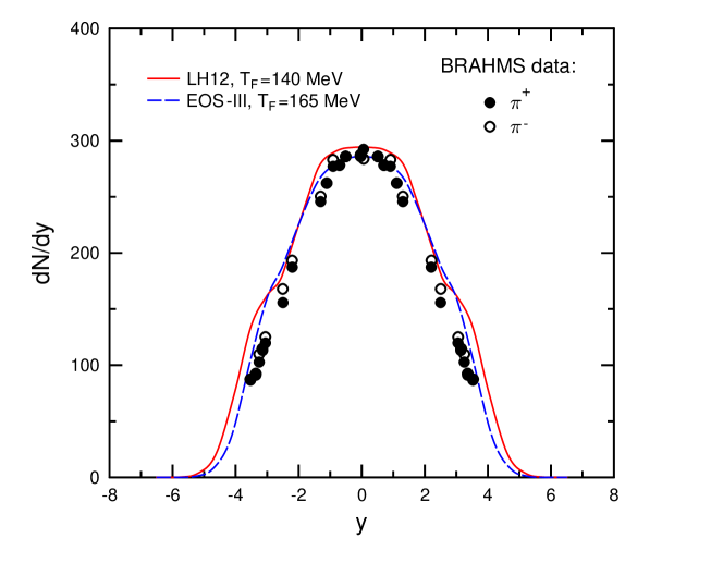
Figure 23: Rapidity distribution of $\pi^{+}$–mesons in central Au+Au collisions at $\sqrt{s_{\scriptscriptstyle NN}}=200$ GeV. Shown are results of hydrodynamical calculations for initial state with parameters $\epsilon_{0}=782$ GeV/fm³, $\eta_{0}=0$, $\sigma=0.1$ . Experimental data are taken from Ref. Bea05 .

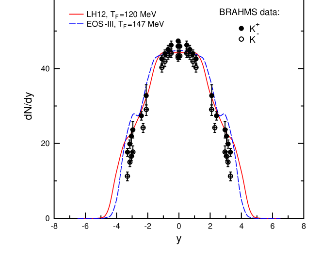
Figure 24: Same as Fig. 23, but for $K^{+}$–meson rapidity distributions.

Now let us consider in more details the Bjorken–like initial conditions corresponding to the table–like profiles ($\sigma=0$) of energy density . In this case the energy density at $\tau=\tau_{0}$ is parametrized as $\epsilon_{0}\hskip 1.0pt\Theta(\eta_{0}-|\eta|)$ . At fixed $\eta_{0}$ the parameter $\epsilon_{0}$ can be determined from the total energy constraint (23). The explicit expression for $\eta_{0}$ as a function of $\epsilon_{0}$ is given by Eq. (26) with $\alpha=0,\,\beta=1$ . Note, that strictly speaking, the Bjorken limit corresponds to infinite total energy and $\eta_{0}\to\infty$ . Our calculations show that deviations from the Bjorken scaling increase with decreasing $\eta_{0}$ .

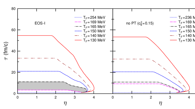
Figure 25: Same as Fig. 12, but for the initial profile with parameters $\epsilon_{0}=7$ GeV/fm³ , $\sigma=0$ , $\eta_{0}=3.34$ .

Figure 25 shows isotherms for a table–like initial state corresponding to the point D in Fig. 4. Similarly to the case of Landau–like initial conditions, these isotherms have parts with inverse slope, but they are much smaller and appear only at large $\eta$ . The calculations show that these parts contribute only to the tails of rapidity distributions.

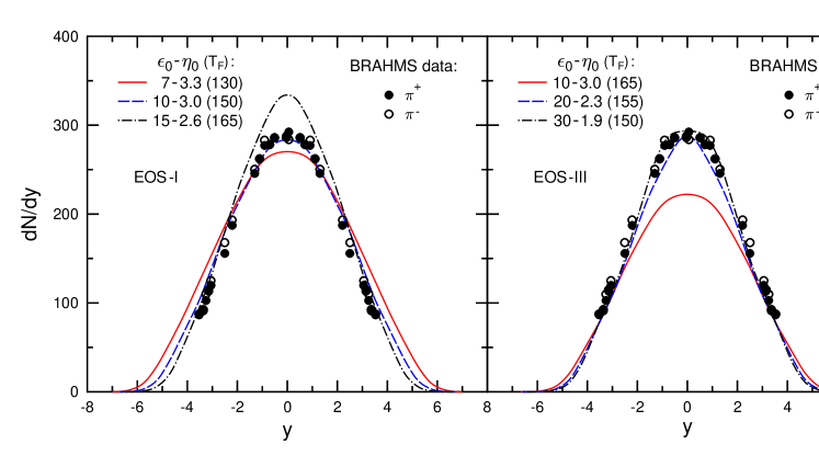
Figure 26: Rapidity distribution of $\pi^{+}$–mesons in central Au+Au collisions at $\sqrt{s_{\scriptscriptstyle NN}}=200$ GeV. Solid, dashed and dashed–dotted curves are calculated for $\sigma=0$ and different values of $\epsilon_{0}$ (in GeV/fm³), $\eta_{0}$ and $T_{F}$ (in MeV). The left (right) panel corresponds to the EOS–I (III). Experimental data are taken from Ref. Bea05 .

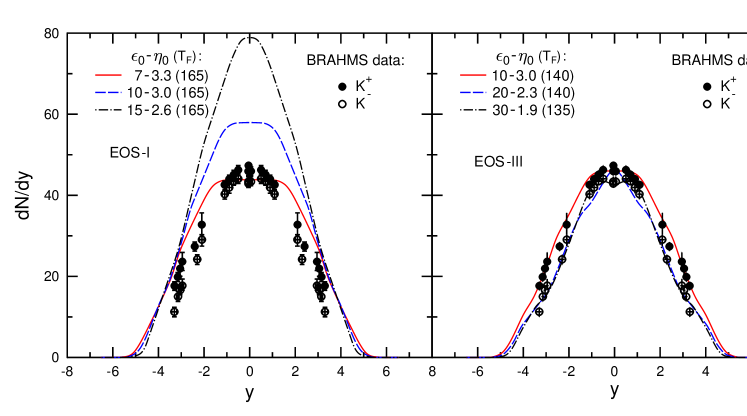
Figure 27: Same as Fig. 26, but for $K^{+}$–meson rapidity distributions.

The pion and kaon rapidity distributions for Bjorken–like initial states are given in Figs. 26– 27. Figure 26 shows the pion rapidity distributions calculated for several values of the parameter $\epsilon_{0}$ and for two EOS s with the phase transition. In all cases the freeze–out temperature is chosen by the best (when possible) fit of BRAHMS data. In accordance with the discussion in Sect. III.2, the pion yield, calculated for fixed initial state, decreases (increases) with raising $T_{F}$ for the EOS–I (III).

The results for kaon spectra are given in Fig. 27. One can see that at $\epsilon_{0}\gtrsim 10$ GeV/fm³ the produced kaon yield is overestimated for the EOS–I at any freeze–out temperatures below $T_{H}=165$ MeV (we do not consider unrealistically small temperatures, $T_{F}\lesssim 50$ MeV). On the other hand, at lower $\epsilon_{0}$ both pion and kaon spectra become too flat at midrapidity. As seen from the right panels of Figs. 26–27, in the case of the EOS–III it is possible to reproduce simultaneously pion and kaon spectra at $\epsilon_{0}\sim 20$ GeV/fm³ . However, for such $\epsilon_{0}$ the freeze–out temperatures for kaons are considerably lower than for pions. This means that kaons are emitted later than pions, which is apparently unrealistic.

On the basis of this analysis we conclude that both the Landau–like and the Bjorken–like initial conditions lead to unsatisfactory results for all considered EOS s.

IV Summary and discussion

In this paper we have generalized Bjorken’s scaling hydrodynamics for finite–size profiles of energy density in pseudorapidity space. The hydrodynamical equations were solved numerically in $\tau-\eta$ coordinates starting from the initial time $\tau_{0}=1$ fm/c until the freeze–out stage. The sensitivity of the final particle distributions to the initial conditions, the freeze–out temperature and the EOS has been investigated. A comparison of $\pi,K,\overline{p}$ rapidity spectra with the BRAHMS data for central Au+Au collisions at $\sqrt{s_{\scriptscriptstyle NN}}=200$ GeV has been made. The best agreement with these data is obtained for initial states with nearly Gaussian profiles of the energy density. In choosing the initial conditions we impose the constraint on the total energy of produced particles known from experimental data Bea04 . It is found that the maximum energy density of the initial state, $\epsilon_{0}$, is sensitive to the parameters of a possible deconfinement phase transition. The BRAHMS data are well reproduced with $\epsilon_{0}$ of about 10 (5) GeV/fm³ for the critical temperature $T_{c}\sim 165\,(190)$ MeV. The only unsatisfactory aspect of these calculations is the prediction of very long freeze–out times, $\sim 50$ fm/c, for pions.

We would like to comment on several points. First, all calculations in this paper are made for $\tau_{0}=1$ fm/c. Of course, one can start the hydrodynamical evolution from an earlier time, i.e. assuming smaller $\tau_{0}$ . In this case one should choose accordingly higher initial energy densities. But $\tau_{0}$ cannot be taken too small, since at very early times the energy is most likely stored in strong chromofields McL94 . The quark–gluon plasma is produced as a result of the decay of these fields. Estimates show that the characteristic decay times are in the range $0.3-1.0$ fm/c. At earlier times the system will contain both the fields as well as produced partons, and the evolution equations will be more complicated, see e.g. Ref. Mis02 .

It is obvious that the Cooper–Frye scenario of the freeze-out process, applied in this paper is too simplified. This was demonstrated e.g. in Ref. Bra99 . One should also bear in mind that the freeze–out temperatures obtained in our model will be modified by the effects of transverse expansion and chemical nonequilibrium. Attempts to construct a more realistic description of the freeze–out have been performed in Refs. Bas00 ; Tea01 , where the transport model was applied to describe evolution of the hadronic phase. In this approach the solution of fluid–dynamical equations is used to obtain initial conditions for hadronic cascade calculations at later stages of matter expansion. We are planning to study these problems in the future.

Appendix A The fluid–dynamical equations in the conservative form

In order to apply the standard flux–corrected transport algorithm Bor73 to solve numerically the equations of fluid dynamics it is necessary to represent them in the conservative form. The following set of equations can be written within the 1+1 dimensional model in the cartesian coordinates $t-z$ (for completeness we consider the general case of nonzero baryon charge)

$$\partial_{t}\bm{u}+\partial_{z}\hskip 1.0pt(\bm{u}v_{z}+\bm{f})+\bm{g}=0\,,$$ (39)

where $z$ and $v_{z}=U^{z}/U^{0}$ are the spacial coordinate and the fluid 3–velocity. The multi–component vector $\bm{u}$ includes the densities of baryon charge ($u_{1}=nU^{0}$), energy ($u_{2}=T^{00}$) and momentum ($u_{3}=T^{0z}$). In the usual space–time representation $\bm{g}$ vanishes and $f_{1}=0$, $f_{2}=Pv_{z},\,f_{3}=P$ .

To rewrite these equations in the light–cone variables, one can perform the Lorentz–transformation of the baryon current $J^{\mu}=nU^{\mu}$ and the energy–momentum tensor $T^{\mu\nu}$ to the frame moving with the rapidity $\eta=\rm{tanh}^{-1}(z/t)$ (this reference frame is marked below by tilde). In particular, $\widetilde{J}^{\,0}=n\cosh{\widetilde{Y}},\widetilde{J}^{z}=n\sinh{\widetilde{Y}}$ and

$$\widetilde{T}^{00}=\epsilon\hskip 1.0pt\cosh^{2}{\widetilde{Y}}+P\sinh^{2}{\widetilde{Y}}\,,$$ (40)

$$\widetilde{T}^{0z}=(\epsilon+P)\hskip 1.0pt\cosh{\widetilde{Y}}\sinh{\widetilde{Y}}\,,$$ (42)

$$\widetilde{T}^{zz}=\epsilon\hskip 1.0pt\sinh^{2}{\widetilde{Y}}+P\cosh^{2}{\widetilde{Y}}\,,$$

where $\widetilde{Y}\equiv Y-\eta$ .

From Eqs. (1)–(2) of the main text we have

$$\partial_{\tau}\widetilde{J}^{\,0}+\partial_{x}\widetilde{J}^{z}+\widetilde{J}^{\,0}/\tau=0\,,$$ (43)

$$\partial_{\tau}\tilde{T}^{00}+\partial_{x}\widetilde{T}^{0z}+(\widetilde{T}^{00}+\widetilde{T}^{zz})/\tau=0\,,$$ (44)

$$\partial_{\tau}\widetilde{T}^{0z}+\partial_{x}\widetilde{T}^{zz}+2\widetilde{T}^{0z}/\tau=0\,,$$ (45)

where $dx=\tau\hskip 1.0ptd\eta$ . These equations are equivalent to Eqs. (5)–(7) of Sect. II.1. One can see that Eqs. (43)–(45) have the form (39) with the replacement $t\to\tau$, $z\to\tau\eta$, $v_{z}\to\rm{tanh}\hskip 1.0pt(Y-\eta)$.

In the baryon–free case $\widetilde{J}^{0}=\widetilde{J}^{z}=0$ and Eq. (43) is trivially satisfied. The ”phoenical” version of SHASTA algorithm Bor73 is used to solve numerically Eqs. (44)–(45) in the rectangle $|\eta|<\eta_{\rm max}$, $\tau_{0}<\tau<\tau_{\rm max}$ of the $\eta-\tau$ plane. Typically we choose $\eta_{\rm max}=10$, $\tau_{\rm max}=200$ fm/c. The grid size $\Delta\eta=1.25\cdot 10^{-2}$ is used in most calculations. For each time step the increment $\Delta\tau$ is found from the requirement $\Delta\tau={\rm min}\hskip 1.0pt(0.1\tau\Delta\eta,\,0.1\,{\rm fm/c})$ . The latter is motivated by the Courant condition for the stability of fluid–dynamical equations in a finite difference approximation. Within the light cone representation this conditions takes the form $\Delta\tau<\Delta x/c_{s}=\tau\Delta\eta/c_{s}$ , where $c_{s}<c$ is the sound velocity.

Appendix B Particle spectra from resonance decay

One can simplify the expressions (30) for spectra of particles produced in resonance decays, having in mind that degeneracy effects in resonance phase–space densities should be small at small $\mu_{F}$ and realistic temperatures $T_{F}\gtrsim 100$ MeV. Therefore, when calculating invariant momentum distributions of resonances, one can approximate the Bose or Fermi functions in Eq. (27) by the corresponding Boltzmann–Jüttner expression:

$$E_{R}\frac{d^{\hskip 1.0pt3}N_{R}}{d^{\hskip 1.0pt3}p_{R}}\simeq\frac{g_{R}}{(2\pi)^{3}}\int d\sigma_{\mu}p_{R}^{\,\mu}\exp\left(\frac{\mu_{F}-p_{R}\hskip 1.0ptU_{F}}{T_{F}}\right)\,,$$ (46)

where $g_{R}$ is the degeneracy factor of the resonance $R$ . Presence of delta–function allows us to easily remove integration over the angle between $\bm{p}_{R}$ and $\bm{p}$ in Eq. (30). Using further the Lorentz–invariance of (30), it is possible to make analytic integration over the resonance energy in the fluid rest frame. The result can be written as

$$E\frac{d^{\hskip 1.0pt3}N_{R\to i}}{d^{\hskip 1.0pt3}p}=\frac{d^{\hskip 1.0pt3}N_{R\to i}}{d^{\hskip 1.0pt2}p_{T}\hskip 1.0ptdy}=\frac{g_{R}b_{R\to i}}{16\pi^{2}}\int\limits_{\displaystyle m_{\rm thr}}^{\infty}d\hskip 1.0ptm_{R}\hskip 1.0pt\frac{m_{R}}{q_{0}}\hskip 1.0ptw\hskip 1.0pt(m_{R})\int d\sigma_{\mu}\left(A\hskip 1.0ptp^{\,\mu}+B\hskip 1.0ptU_{F}^{\mu}\right)\,.$$ (47)

The Lorentz–scalars $A$ and $B$ in the r.h.s. are determined as follows

$$A=\frac{T_{F}}{p^{\,\prime 3}}\left[E^{\,\prime}(E_{-}+T_{F})-m_{R}E_{0\hskip 1.0pti}\right]e^{\,\displaystyle(\mu_{F}-E_{-})/T_{F}}-(E_{-}\to E_{+})\,,$$ (48)

$$B=\frac{T_{F}}{p^{\,\prime 3}}\left[E^{\,\prime}m_{R}E_{0\hskip 1.0pti}-m_{i}^{2}(E_{-}+T_{F})\right]e^{\,\displaystyle(\mu_{F}-E_{-})/T_{F}}-(E_{-}\to E_{+})\,,$$ (49)

where $E^{\,\prime}=\sqrt{m_{i}^{2}+p^{\,\prime 2}}\equiv p\hskip 1.0ptU_{F}=m_{T}\cosh(y-Y_{F})$ and $E_{\pm}\equiv m_{R}\hskip 1.0pt(E_{0\hskip 1.0pti}E^{\,\prime}\pm q_{0}p^{\,\prime})/m_{i}^{2}$ .

In most cases, when calculating contributions of resonance decays we apply the zero–width approximation, i.e. substitute $w\hskip 1.0pt(m_{R})=\delta\hskip 1.0pt(m_{R}-\overline{m}_{R})$ , where $\overline{m}_{R}$ is the central mass value presented in Ref. PDG04 for the resonance $R$ . However, we take into account the nonzero width of $\rho$–mesons. Following Ref. Sol90 , we apply the parametrization

$$w\hskip 1.0pt(m_{R})=\frac{C\gamma(m_{R})}{(m_{R}^{2}-\overline{m}_{R}^{\,2})^{2}+\gamma^{2}(m_{R})}\,,$$ (50)

Here the constant $C$ is taken from the normalization condition, $\int\limits_{m_{\rm thr}}^{\infty}d\hskip 1.0ptm_{R}w\hskip 1.0pt(m_{R})=1$ , and

$$\gamma(m_{R})=\xi\frac{m_{R}\hskip 1.0ptq_{0}^{3}}{q_{0}^{2}+\Lambda^{2}}\,,$$ (51)

where $q_{0}=\sqrt{m_{R}^{2}/4-m_{\pi}^{2}}$ . The numerical values Sol90

$$\overline{m}_{R}=770\,{\rm MeV},~{}~{}\Lambda=159\,{\rm MeV},~{}~{}\xi=0.5\,,$$ (52)

are used to calculate feeding from $\rho$–meson decays.