Neutrinos and electrons in background matter: a new approach

Abstract

We present a rather powerful method in investigations of different phenomena that can appear when neutrinos and electrons are moving in the background matter. This method is based on the use of the modified Dirac equations for the particles wave functions, in which the correspondent effective potentials that account for the matter influence on particles are included. The developed approach establishes a basis for investigation of different phenomena which can arise when neutrinos and electrons move in dense media, including those peculiar for astrophysical and cosmological environments. The approach developed is similar to the Furry representation of quantum electrodynamics, widely used for description of particles interactions in the presence of external electromagnetic fields, and it works when a macroscopic amount of the background particles are confined within the scale of a neutrino or electron de Broglie wave lengths. We consider the modified Dirac equations for neutrinos (of both Dirac and Majorana types) and electrons having the standard model interactions with the background matter, however generalization to extensions of the standard model is just straightforward. To illustrate how the developed method works, we elaborate the quantum theories of the spin light of neutrino ($SL\nu$) and spin light of electron ($SLe$) in matter.

1 Introduction

The neutrino is a very fascinating particle which has remained under the focus of intensive investigations, both theoretical an experimental, for a couple of decades. These studies have given evidence of an ultimate relation between the knowledge on neutrino properties and understanding of fundamentals of particle physics. The birth of the neutrino (this particle was predicted by W.Pauli in 1930) was due to an attempt to explain the continuous spectrum of beta-particles and correspondently to find “a way out for saving the law of conservation of energy” [1]. This new particle, called at first the “neutron” and then renamed the “neutrino”, was an essential counterpart of the first model for the weak interactions (E.Fermi, 1934). The further important milestones of particle physics, such as the parity nonconcervation (T.Lee, C.Yang, 1956) and the $V-A$ model of the local weak interactions (E.Sudarshan, R.Marshak, 1956; R.Feynman, M.Gell-Mann, 1958), as well as the structure of the Glashow-Weinberg-Salam standard model, were based on the clarification of the specific properties of the neutrino. To summarize the present status of the neutrino physics we quote [2]: “Recent discovery of flavour conversion of solar, atmospheric, reactor and accelerator neutrinos have conclusively established that neutrinos have nonzero mass and they mix among themselves much like quarks, providing the first evidence of new physics beyond the standard model”. Thus, it has happened not once that a novel discovery in neutrino physics stimulates a far-reaching consequences in the theory of particle interactions.

The neutrino plays a crucial role in particle physics because it is a “tiny” particle. Indeed, the scale of neutrino mass is much lower than ones of the charged fermions ($m_{\nu_{f}}<<m_{f},\ \ f=e,\mu,\tau$). In addition to electric neutrality and very small (if non-zero) magnetic moment, the weak interactions of neutrino with other particles are really weak. That is a reason for the neutrino to appear under the focus of researchers during the latest stages of a particular particle physics paradigm evolution when all of the “principal” phenomena have been already observed and theoretically described. That is why the neutrino has often provided a kind of a bridge to “new physics”.

In general, the neutrino most easily demonstrates its properties when it is subjected to the influence of extreme external conditions which can be provided by the presence of dense matter or strong external electromagnetic fields. A crucial importance of external influence on neutrinos is vividly demonstrated by the fact that the resonant neutrino flavour oscillations in matter [3] has been proven to be the mechanism for solving the solar neutrino problem. The resonant neutrino spin (or spin-flavour) oscillations in matter under the influence of external transversal magnetic field [4] have also important consequences in astrophysics and cosmology (see, for instance, [5]). In the presence of matter a neutrino dispersion relation is modified [6, 7, 8], in particular, it has a minimum at nonzero momentum [9, 10]. As it was shown in [6, 7, 8], the standard result for the MSW effect can be derived using a modified Dirac equation for the neutrino wave function with a matter potential proportional to the density being added. The problem of a neutrino mass generation in different media was also studied [12, 13] on the basis of modified Dirac equations for neutrinos. On the same basis spontaneous neutrino-pair creation in matter was also studied [14, 15, 16] (neutrino-pair creation in a perturbative way has been recently discussed in [17]).

The aim of this paper is to present a rather powerful method in investigations of different phenomena that can appear when neutrinos are moving in the background matter [18, 19]. In addition, we also demonstrate how this method can be applied to electrons moving in background matter [20, 21]. The approach developed establishes a basis for investigation of different phenomena which can arise when neutrinos and electrons move in dense media, including those peculiar for astrophysical and cosmological environments.

The method discussed is based on the use of the modified Dirac equations for the particles wave functions, in which the correspondent effective potentials that account for the matter influence on the particles are included. It is similar to the Furry representation [22] in quantum electrodynamics, widely used for description of particles interactions in the presence of external electromagnetic fields.

In quantum electrodynamics, as well as in other more general models of interaction, there are two different approaches to the problem of particles interactions in the presence of external electromagnetic fields. Within the first approach, in the presence of external field one has to substitute the four-potential of the external field $A_{\mu}(x)$ by $A^{\prime}_{\mu}(x)$ in accordance with

$$A^{\prime}_{\mu}(x)=A_{\mu}+A_{\mu}^{ext}(x),$$ (1)

where $A_{\mu}(x)$ is the quantized radiation field, and $A_{\mu}^{ext}(x)$ is the potential of the external field that is a given function of the four-coordinate $x$. The appropriate Feynman diagram techniques, after the external field potential $A_{\mu}^{ext}(x)$ being substituted into the interaction Hamiltonian, can be developed. This approach implies that the external filed is accounted for within the perturbation-theory expansion and additional lines on the Feynman diagrams, which stand for interaction with the external field, appears [23]. Note that applications of the approach discussed is limited by the strength of the external field. For instance, it can not be used in the case very strong electromagnetic fields or in the case when non-liner over the external field effects are important.

There is another approach to the problem of particles interaction in the presence of external electromagnetic fields which enables one to account for the external field effect exactly, rather than within the perturbation-series expansion discussed above. In this techniques, known in quantum electrodynamics as the Furry representation, the evolution operator $U_{F}(t_{1},t_{2})$, which determines the matrix element of the process, is represented in the usual form

$$U_{F}(t_{1},t_{2})=Texp\bigg{[}-i\int\limits_{t_{1}}^{t_{2}}j_{\mu}(x)A^{\mu}{d}x\bigg{]},$$ (2)

where $A_{\mu}(x)$ is the quantized part of the potential corresponding to the radiation field, which is accounted within the perturbation-series techniques. At the same time, the charged particles current is represented in the form

$$j_{\mu}(x)={e\over 2}\big{[}\overline{\Psi}_{F}\gamma_{\mu},\Psi_{F}\big{]},$$ (3)

where $\Psi_{F}$ are the exact solutions of the quantum wave equation for the charged particles (that is the Dirac equation in the case of an electron) in the presence of external electromagnetic field given by the classical non-quantized potential $A_{\mu}^{ext}(x)$. Note that within this approach the interaction of charged particles with the external electromagnetic field is taken into account exactly while the radiation field is allowed for by perturbation-series expansion techniques. A detailed discussion of this method can be found in [24].

Note that our focus in this paper is on the standard model interactions of neutrinos and electrons in the background matter (i.e., we consider the standard model processes with participation of neutrinos and electrons that proceed under the influence of the standard-model-interacting matter background). It worth to be mentioned, that on the same ideological basis (which implies the use of the exact solutions of the corresponding Dirac equations) different processes with neutrinos and electrons beyond the standard model (and also with non-standard model interactions with an environment) were considered in the literature [11, 25, 26].

Here below we start with the discussion on the form of the modified Dirac equation for the neutrino wave function in the presence of the background matter. We consider the two possibilities that are provided by the use of the modified Dirac-Pauli and modified Dirac equations. For both cases we explicitly evaluate the exact solutions for the wave functions and derive the neutrino energy spectra in the background matter. Then we also consider the particular case of the Majorana neutrino and determine the energy spectrum for this case. For the Dirac neutrino, using the obtained neutrino energy spectrum, we discuss several interesting phenomena, such as neutrino trapping, neutrino reflection and neutrino-antineutrino pair production and annihilation that can appear at the boundary of media with different densities. Then we demonstrate how the evaluated neutrino quantum states in matter (the exact neutrino wave functions and energy spectrum in matter) can be used for investigation of different processes in the presence of matter. As an example, we develop the quantum theory of the spin light of neutrino ($SL\nu$), a new type of the electromagnetic radiation that can be emitted by the neutrino moving in the background matter. In the final section of the paper, we derive the modified Dirac equation for an electron moving in the background matter and obtain in explicit form the electron wave function and energy spectrum. On this bases we predict a new type of radiation that can be emitted by the electron moving in matter (we have termed this radiation as “spin light of electron” in matter [20, 21]).

2 Neutrino wave function and energy spectrum in matter

In this section we discuss two quantum equations, the modified Dirac-Pauli and modified Dirac ones, for a massive neutrino wave function in the background matter. The two wave functions and energy spectra, that correspond to these two equations, in general do not coincide. However, for the relativistic neutrino and in the linear approximation over the matter density the two energy spectra lead to equal results for the energy difference of the left-handed and right-handed neutrino states. So that, in the lowest approximation over the matter density, the results for the $SL\nu$ photon energy, rate and power obtained on the basis of the two equations discussed (see Section 3) are equal.

2.1 Modified Dirac-Pauli equation for neutrino in matter

To derive the quantum equation for a neutrino wave function in the background matter we start with the well-known Dirac-Pauli equation for a neutral fermion with non-zero magnetic moment. For a massive neutrino moving in an electromagnetic field $F_{\mu\nu}$ this equation is given by

$$\Big{(}i\gamma^{\mu}\partial_{\mu}-m-\frac{\mu}{2}\sigma^{\mu\nu}F_{\mu\nu}\Big{)}\Psi(x)=0,$$ (4)

where $m$ and $\mu$ are the neutrino mass and magnetic moment [27] , $\sigma^{\mu\nu}=i/2\big{(}\gamma^{\mu}\gamma^{\nu}-\gamma^{\nu}\gamma^{\mu}\big{)}$. It worth to be noted here that Eq.(4) can be obtained in the linear approximation over the electromagnetic field from the Dirac-Schwinger equation, which in the case of the neutrino takes the following form [28]:

$$(i\gamma^{\mu}\partial_{\mu}-m)\Psi(x)=\ \int M^{F}(x^{\prime},x)\Psi(x^{\prime})dx^{\prime},$$ (5)

where $M^{F}(x^{\prime},x)$ is the neutrino mass operator in the presence of the external electromagnetic field.

For the case of the external magnetic filed, the Hamiltonian form of the equation (4) reads

$$i\frac{\partial}{\partial t}\Psi({\bf r},t)=\hat{H}_{F}\Psi({\bf r},t),$$ (6)

where

$$\hat{H}_{F}=\hat{\bm{\alpha}}{\bf p}+\hat{\beta}m+\hat{V}_{F},\hat{V}_{F}=-\mu\hat{\beta}{\bf{\hat{\Sigma}}}{\bf B},$$ (7)

and ${\bf B}$ is the magnetic field vector. We use the Pauli-Dirac representation of the Dirac matrices $\hat{\bm{\alpha}}$ and $\hat{\beta}$, in which

$$\hat{\bm{\alpha}}=\begin{pmatrix}{0}&{\hat{\bm{\sigma}}}\\ {\hat{\bm{\sigma}}}&{0}\end{pmatrix}=\gamma_{0}{\bm{\gamma}},\ \ \ \hat{\beta}=\begin{pmatrix}{1}&{0}\\ {0}&{-1}\end{pmatrix}=\gamma_{0},\ \ {\hat{\bm{\Sigma}}}=\begin{pmatrix}{\hat{\bm{\sigma}}}&{0}\\ {0}&{\hat{\bm{\sigma}}}\end{pmatrix},$$ (8)

where ${\hat{\bm{\sigma}}}=({\sigma}_{1},{\sigma}_{2},{\sigma}_{3})$ and $\sigma$ denotes the Pauli matrixes.

Recently in a series of our papers [30, 31, 32, 33] we have developed the quasi-classical approach to the massive neutrino spin evolution in the presence of external fields and background matter. In particular, we have shown that the well known Bargmann-Michel-Telegdi (BMT) equation [34] of the electrodynamics can be generalized for the case of a neutrino moving in the background matter and being also under the influence of external electromagnetic fields. The proposed new equation for a neutrino, which simultaneously accounts for the electromagnetic interaction with external fields and also for the weak interaction with particles of the background matter, was obtained from the BMT equation by the following substitution of the electromagnetic field tensor $F_{\mu\nu}=(\bf E,\bf B)$:

$$F_{\mu\nu}\rightarrow E_{\mu\nu}=F_{\mu\nu}+G_{\mu\nu},$$ (9)

where the tensor $G_{\mu\nu}=(-{\bf P},{\bf M})$ accounts for the neutrino interactions with particles of the environment. The substitution (9) implies that in the presence of matter the magnetic $\bf B$ and electric $\bf E$ fields are shifted by the vectors $\bf M$ and $\bf P$, respectively:

$$\bf B\rightarrow\bf B+\bf M,\ \ \bf E\rightarrow\bf E-\bf P.$$ (10)

We have also shown how to construct the tensor $G_{\mu\nu}$ with the use of the neutrino speed, matter speed, and matter polarization four-vectors.

Now let us consider the case of a neutrino moving in matter without any electromagnetic field in the background. The quantum equation for the neutrino wave function can be obtained from (4) with application of the substitution (9) which now becomes

$$F_{\mu\nu}\rightarrow G_{\mu\nu}.$$ (11)

Thus, we get the quantum equation for the neutrino wave function in the presence of the background matter in the form [35]

$$\Big{(}i\gamma^{\mu}\partial_{\mu}-m-\frac{\mu}{2}\sigma^{\mu\nu}G_{\mu\nu}\Big{)}\Psi(x)=0,$$ (12)

that can be regarded as the modified Dirac-Pauli equation. The generalization of this equation for the case when an electromagnetic field is present in the environment, in addition to the background matter, is just straightforward. In particular, the case of external magnetic field is considered below.

The detailed discussion on the evaluation of the tensor $G_{\mu\nu}$ is given in [30, 31, 33]. We consider here, for simplicity, the case of the unpolarized matter composed of the only one type of fermions of a constant density. For a background of only electrons we get

$$G^{\mu\nu}=\gamma\rho^{(1)}n\begin{pmatrix}{0}&{0}&{0}&{0}\\ {0}&{0}&{-\beta_{3}}&{\beta_{2}}\\ {0}&{\beta_{3}}&{0}&{-\beta_{1}}\\ {0}&{-\beta_{2}}&{\beta_{1}}&{0}\end{pmatrix},\gamma=(1-{\bm{\beta}}^{2})^{-1/2},\rho^{(1)}=\frac{\tilde{G}_{F}}{2\sqrt{2}\mu},\tilde{G}_{F}=G_{F}(1+4\sin^{2}\theta_{W}),$$ (13)

where ${\bm{\beta}}=(\beta_{1},\beta_{2},\beta_{3})$ is the neutrino three-dimensional speed, $n$ denotes the number density of the background electrons. From (13) and the two equations, (4) and (12), it is possible to see that the term $\gamma\rho^{(1)}n{\bm{\beta}}$ in (12) plays the role of the magnetic field $\bf B$ in (4). Therefore, the Hamiltonian form of (12) is

$$i\frac{\partial}{\partial t}\Psi({\bf r},t)=\hat{H}_{G}\Psi({\bf r},t),$$ (14)

where

$$\hat{H}_{G}=\hat{\bm{\alpha}}{\bf p}+\hat{\beta}m+\hat{V}_{G},$$ (15)

and

$$\hat{V}_{G}=-\mu\frac{\rho^{(1)}n}{m}\hat{\beta}{\bf\Sigma}{\bf p},$$ (16)

here $\bf p$ is the neutrino momentum. From (16) it is just straightforward that the potential energy in matter depends on the neutrino helicity.

The form of the Hamiltonian (15) ensures that the operators of the momentum, $\hat{\bf p}$, and helicity, ${\bf\Sigma}{\bf p}/p$, are integrals of motion. That is why for the stationary states we can write

$$\Psi({\bf r},t)=e^{-i(Et-{\bf p}{\bf r})}u({\bf p},E),\ \ \ u({\bf p},E)=\begin{pmatrix}{\varphi}\\ {\chi}\end{pmatrix},$$ (17)

where $u({\bf p},E)$ is independent on the coordinates and time and can be expressed in terms of the two-component spinors $\varphi$ and $\chi$. Substituting (43) into Eq.(14), we get the two equations

$$({\bm{\sigma}}{\bf p})\chi-\big{(}E-m+\alpha({\bm{\sigma}}{\bf p})\big{)}\varphi=0,\ \ \ ({\bm{\sigma}}{\bf p})\varphi-\big{(}E-m+\alpha({\bm{\sigma}}{\bf p})\big{)}\chi=0.$$ (18)

Suppose that $\varphi$ and $\chi$ satisfy the following equations,

$$({\bm{\sigma}}{\bf p})\varphi=sp\varphi,\ \ ({\bm{\sigma}}{\bf p})\chi=sp\chi,$$ (19)

where $s=\pm 1$ specify the two neutrino helicity states. Upon the condition that the set of Eqs.(18) has a non-trivial solution, we arrive to the energy spectrum of a neutrino moving in the background matter:

$$E={\sqrt{{\bf p}^{2}(1+\alpha^{2})+m^{2}-2\alpha mps}},\ \ \ \ \alpha=\frac{\mu\rho^{(1)}}{m}n=\frac{1}{2\sqrt{2}}{\tilde{G}}_{F}\frac{n}{m}.$$ (20)

It is important that the the neutrino energy in the background matter depends on the state of the neutrino longitudinal polarization (helicity), i.e. the left-handed and right-handed neutrinos with equal momentum have different energies.

The obtained expression (20) for the neutrino energy can be transformed to the form

$$E=\sqrt{{\bf p}^{2}+m^{2}\Big{(}1-s\frac{\alpha p}{m}\Big{)}^{2}}.$$ (21)

It is easy to see that the energy spectrum of a neutrino in vacuum, which is derived on the basis of the Dirac equation, is modified in the presence of matter by the formal shift of the neutrino mass

$$m\rightarrow m\Big{(}1-s\frac{\alpha p}{m}\Big{)}.$$ (22)

The procedure, similar to one used for the derivation of the solution of the Dirac equation in vacuum, can be adopted for the case of the neutrino moving in matter. We apply this procedure to equation (14) and arrive to the final form of the wave function of a neutrino moving in the background matter:

$$\Psi_{{\bf p},s}({\bf r},t)=\frac{e^{-i(Et-{\bf p}{\bf r})}}{2L^{\frac{3}{2}}}\begin{pmatrix}{\sqrt{1+\frac{m-s\alpha p}{E}}}\ \sqrt{1+s\frac{p_{3}}{p}}\\ {s\sqrt{1+\frac{m-s\alpha p}{E}}}\ \sqrt{1-s\frac{p_{3}}{p}}\ \ e^{i\delta}\\ {s\sqrt{1-\frac{m-s\alpha p}{E}}}\ \sqrt{1+s\frac{p_{3}}{p}}\\ {\sqrt{1-\frac{m-s\alpha p}{E}}}\ \ \sqrt{1-s\frac{p_{3}}{p}}\ e^{i\delta}\end{pmatrix},$$ (23)

where $L$ is the normalization length and $\delta=\arctan p_{y}/p_{x}$. In the limit of vanishing matter density, when $\alpha\rightarrow 0$, the wave function of (23) transforms to the vacuum solution of the Dirac equation.

Calculations on the basis of the modified Dirac-Pauli equation (12) enables us to reproduce, to the lowest order of the expansion over the matter density, the correct energy difference between the two neutrino helicity states in matter . On the basis of the obtained neutrino energy spectrum (20), in the low matter density limit $\alpha\frac{pm}{E_{0}^{2}}\ll 1$, we can reproduce the correct result for the energy difference $\Delta E=E(s=-1)-E(s=+1)$ of the two neutrino helicity states:

$$\Delta E\approx 2m\alpha\frac{p}{E_{0}},$$ (24)

where we use the notation $E_{0}=\sqrt{p^{2}+m^{2}}$. Therefore, for the relativistic neutrinos one can derive, using (16), the probability of the neutrino spin oscillations $\nu_{L}\leftrightarrow\nu_{R}$ in transversal magnetic field with the correct form of the matter term [4] (for the further details see Section 2.2).

2.2 Modified Dirac-Pauli equation in magnetized and polarized matter

We should like to note that it is possible to generalize the Dirac-Pauli equation (4) (or (12)) for the case when a neutrino is moving in the magnetized background matter. For this case (i.e., when the effects of matter and magnetic field on neutrino have to be accounted for) the modified Dirac-Pauli equation is [35]

$$\Big{\{}i\gamma^{\mu}\partial_{\mu}-m-\frac{\mu}{2}\sigma^{\mu\nu}(F_{\mu\nu}+G_{\mu\nu})\Big{\}}\Psi(x)=0,$$ (25)

where the magnetic field $\bf B$ enters through the tensor $F_{\mu\nu}$. The neutrino energy in the magnetized matter can be obtained from (20) by the following redefinition

$$\alpha\rightarrow\alpha^{\prime}=\alpha+\frac{\mu B_{\parallel}}{p},$$ (26)

where $B_{\parallel}=({\bf B}{\bf p})/p$. Thus, the neutrino energy in this case reads

$$E=\sqrt{{\bf p}^{2}+m^{2}\Big{(}1-s\frac{\alpha p+\mu B_{\parallel}}{m}\Big{)}^{2}}.$$ (27)

For the relativistic neutrinos the expression of Eq.(27) gives, in the linear approximation over the matter density and the magnetic field strength, the correct value (see [30, 33]) for the energy difference of the two opposite helicity states in the magnetized matter:

$$\Delta_{eff}={{\tilde{G}}_{F}\over\sqrt{2}}n+2{\mu B_{\parallel}\over\gamma}.$$ (28)

On this basis we can also consider the neutrino spin oscillations in the presence of non-moving matter being under the influence of an arbitrary constant magnetic field ${\bf B}={\bf B}_{\parallel}+{\bf B}_{\perp}$, here $\bf B_{\perp}$ is the transversal to the neutrino momentum component of the external field. In the adiabatic approximation the probability of the oscillations $\nu_{L}\leftrightarrow\nu_{R}$ can be written in the form,

$$P_{\nu_{L}\rightarrow\nu_{R}}(x)=\sin^{2}2\theta_{eff}\sin^{2}{\pi x\over L_{eff}},$$ (29)

$$sin^{2}2\theta_{eff}={E^{2}_{eff}\over{E^{2}_{eff}+\Delta^{2}_{eff}}},L_{eff}={2\pi\over\sqrt{E^{2}_{eff}+\Delta^{2}_{eff}}},$$ (30)

where $E_{eff}=2\mu B_{\perp}$ (terms $\sim\gamma^{-1}$ are omitted here), and $x$ is the distance travelled by the neutrino. The obtained expression for the oscillation probability confirms our previous result of refs.[30, 33].

Let us now shortly discuss the effect of matter polarization. Consider the case of matter composed of electrons in the presence of such strong background magnetic field so that the following condition is valid

$$B>\frac{p_{F}^{2}}{2e},$$ (31)

where $p_{F}=\sqrt{\mu^{2}-m^{2}_{e}}$, $\mu$ and $m_{e}$ are, respectively, the Fermi momentum, chemical potential, and mass of electrons. Then all of the electrons occupy the lowest Landau level (see, for instance, [36]), therefore the matter is completely polarized in the direction opposite to the unit vector $\frac{{\bf B}}{B}$. From the general expression for the tensor $G_{\mu\nu}$ (see the second paper of [30]) we get

$$G^{\mu\nu}=\gamma n\left\{\rho^{(1)}\begin{pmatrix}{0}&{0}&{0}&{0}\\ {0}&{0}&{-\beta_{3}}&{\beta_{2}}\\ {0}&{\beta_{3}}&{0}&{-\beta_{1}}\\ {0}&{-\beta_{2}}&{\beta_{1}}&{0}\end{pmatrix}+\rho^{(2)}\begin{pmatrix}{0}&{-\beta_{2}}&{\beta_{1}}&{0}\\ {\beta_{2}}&{0}&{-\beta_{0}}&{0}\\ {-\beta_{1}}&{\beta_{0}}&{0}&{0}\\ {0}&{0}&{0}&{0}\end{pmatrix}\right\},$$ (32)

$$\rho^{(2)}=-\frac{{G}_{F}}{2\sqrt{2}\mu}.$$

Thus, the modified Dirac-Pauli equation (25) with the tensor $G_{\mu\nu}$ given by (32) can be used for description of the neutrino motion in magnetized and totally polarized (parallel or anti-parallel to the magnetic field vector $\bm{B}$ direction) matter. The neutrino energy in such a case can be obtained from (20) by the following redefinition

$$\alpha\rightarrow{\tilde{\alpha}}=\alpha\left[1-\frac{sign\left(\frac{B_{\parallel}}{B}\right)}{1+\sin^{2}4\theta_{W}}\right]+\frac{\mu B_{\parallel}}{p}.$$ (33)

In Eq.(33), the second term in brackets accounts for the effect of the matter polarization. It follows, that the effect of the matter polarization can reasonably change the total matter contribution to the neutrino energy (27) (see also [36]).

3 Modified Dirac equation for neutrino in matter

In [18] (see also [19, 20]) we derived the modified Dirac equation for the neutrino wave function exactly accounting for the neutrino interaction with matter. Let us consider the case of matter composed of electrons, neutrons, and protons and also suppose that the neutrino interaction with background particles is given by the standard model supplied with the singlet right-handed neutrino. The corresponding addition to the effective interaction Lagrangian is given by

$$\Delta L_{eff}=-f^{\mu}\Big{(}\bar{\nu}\gamma_{\mu}{1+\gamma^{5}\over 2}\nu\Big{)},\ \ f^{\mu}={\sqrt{2}G_{F}}\sum\limits_{f=e,p,n}j^{\mu}_{f}q^{(1)}_{f}+\lambda^{\mu}_{f}q^{(2)}_{f},$$ (34)

where

$$q^{(1)}_{f}=(I_{3L}^{(f)}-2Q^{(f)}\sin^{2}\theta_{W}+\delta_{ef}),\ q^{(2)}_{f}=-(I_{3L}^{(f)}+\delta_{ef}),\ \delta_{ef}=\left\{\begin{tabular}[]{l l}1&for {\it f=e},\\ 0&for {\it f=n, p}.\\ \end{tabular}\right.$$ (35)

Here $I_{3L}^{(f)}$ and $Q^{(f)}$ are, respectively, the values of the isospin third components and electric charges of the particles of matter ($f=e,n,p$). The corresponding currents $j_{f}^{\mu}$ and polarization vectors $\lambda_{f}^{\mu}$ are

$$j_{f}^{\mu}=(n_{f},n_{f}{\bf v}_{f}),\ \ \ \lambda_{f}^{\mu}=\Bigg{(}n_{f}({\bm{\zeta}}_{f}{\bf v}_{f}),n_{f}{\bm{\zeta}}_{f}\sqrt{1-v_{f}^{2}}+{{n_{f}{\bf v}_{f}({\bm{\zeta}}_{f}{\bf v}_{f})}\over{1+\sqrt{1-v_{f}^{2}}}}\Bigg{)},$$ (36)

where $\theta_{W}$ is the Weinberg angle. In the above formulas (36), $n_{f}$, ${\bf v}_{f}$ and ${\bm{\zeta}}_{f}\ (0\leq|{\bm{\zeta}}_{f}|^{2}\leq 1)$ stand, respectively, for the invariant number densities, average speeds and polarization vectors of the matter components. A detailed discussion on the meaning of these characteristics can be found in [30, 31, 32, 33]. Using the standard model Lagrangian with the extra term (34), we derive the modified Dirac equation for the neutrino wave function in matter:

$$\Big{\{}i\gamma_{\mu}\partial^{\mu}-\frac{1}{2}\gamma_{\mu}(1+\gamma_{5})f^{\mu}-m\Big{\}}\Psi(x)=0.$$ (37)

This is the most general form of the equation for the neutrino wave function in which the effective potential $V_{\mu}=\frac{1}{2}(1+\gamma_{5})f_{\mu}$ includes both the neutral and charged current interactions of the neutrino with the background particles and which could also account for effects of matter motion and polarization. It should be mentioned that other modifications of the Dirac equation were previously used in [6]-[13] for studies of the neutrino dispersion relations, neutrino mass generation and neutrino oscillations in the presence of matter. Note that the corresponding quantum wave equation for a Majorana neutrino can be obtained from (37) via the substitution $1+\gamma_{5}\rightarrow 2\gamma_{5}$ (see Section 3.1 below and also [37, 38]).

In the further discussion below we consider the case when no electromagnetic field is present in the background. We also suppose that the matter is unpolarized, $\lambda^{\mu}=0$. Therefore, the term describing the neutrino interaction with the matter is given by

$$f^{\mu}=\frac{\tilde{G}_{F}}{\sqrt{2}}(n,n{\bf v}),$$ (38)

where we use the notation $\tilde{G}_{F}={G}_{F}(1+4\sin^{2}\theta_{W})$.

In the rest frame of the matter the Hamiltonian form of the equation (37) can be written as

$$i\frac{\partial}{\partial t}\Psi({\bf r},t)=\hat{H}_{matt}\Psi({\bf r},t),$$ (39)

where

$$\hat{H}_{matt}=\hat{\bm{\alpha}}{\bf p}+\hat{\beta}m+\hat{V}_{matt},$$ (40)

and

$$\hat{V}_{matt}=\frac{1}{2\sqrt{2}}(1+\gamma_{5}){\tilde{G}}_{F}n.$$ (41)

The form of the Hamiltonian (40) implies that the operators of the momentum, $\hat{\bf p}$, and longitudinal polarization, ${\hat{\bf\Sigma}}{\bf p}/p$, are the integrals of motion. So that, in particular, we have

$$\frac{{\hat{\bf\Sigma}}{\bf p}}{p}\Psi({\bf r},t)=s\Psi({\bf r},t),\ \ {\hat{\bm{\Sigma}}}=\begin{pmatrix}{\hat{\bm{\sigma}}}&{0}\\ {0}&{\hat{\bm{\sigma}}}\end{pmatrix},$$ (42)

where the values $s=\pm 1$ specify the two neutrino helicity states, $\nu_{+}$ and $\nu_{-}$. In the relativistic limit the negative-helicity neutrino state is dominated by the left-handed chiral state ($\nu_{-}\approx\nu_{L}$), whereas the positive-helicity state is dominated by the right-handed chiral state ($\nu_{+}\approx\nu_{R}$).

For the stationary states of the equation (37) we get

$$\Psi({\bf r},t)=e^{-i(E_{\varepsilon}t-{\bf p}{\bf r})}u({\bf p},E_{\varepsilon}),$$ (43)

where $u({\bf p},E_{\varepsilon})$ is independent on the coordinates and time. Upon the condition that the equation (37) has a non-trivial solution, we arrive to the energy spectrum of a neutrino moving in the background matter:

$$E_{\varepsilon}=\varepsilon{\sqrt{{\bf p}^{2}\Big{(}1-s\alpha\frac{m}{p}\Big{)}^{2}+m^{2}}+\alpha m},$$ (44)

where we use the notation

$$\alpha=\frac{1}{2\sqrt{2}}{\tilde{G}}_{F}\frac{n}{m}.$$ (45)

The quantity $\varepsilon=\pm 1$ splits the solutions into the two branches that in the limit of the vanishing matter density, $\alpha\rightarrow 0$, reproduce the positive and negative-frequency solutions, respectively. It is also important to note that the neutrino energy in the background matter depends on the state of the neutrino longitudinal polarization, i.e. in the relativistic case the left-handed and right-handed neutrinos with equal momenta have different energies.

We get the exact solution of the modified Dirac equation in the form [18]

$$\Psi_{\varepsilon,{\bf p},s}({\bf r},t)=\frac{e^{-i(E_{\varepsilon}t-{\bf p}{\bf r})}}{2L^{\frac{3}{2}}}\begin{pmatrix}{\sqrt{1+\frac{m}{E_{\varepsilon}-\alpha m}}}\ \sqrt{1+s\frac{p_{3}}{p}}\\ {s\sqrt{1+\frac{m}{E_{\varepsilon}-\alpha m}}}\ \sqrt{1-s\frac{p_{3}}{p}}\ \ e^{i\delta}\\ {s\varepsilon\sqrt{1-\frac{m}{E_{\varepsilon}-\alpha m}}}\ \sqrt{1+s\frac{p_{3}}{p}}\\ {\varepsilon\sqrt{1-\frac{m}{E_{\varepsilon}-\alpha m}}}\ \ \sqrt{1-s\frac{p_{3}}{p}}\ e^{i\delta}\end{pmatrix},$$ (46)

where the energy $E_{\varepsilon}$ is given by (44), $L$ is the normalization length and $\delta=\arctan{p_{2}/p_{1}}$. In the limit of vanishing density of matter, when $\alpha\rightarrow 0$, the wave function (46) transforms to the vacuum solution of the Dirac equation.

The quantum equation (37) for a neutrino in the background matter with the obtained exact solution (46) and energy spectrum (44) establish a basis for a very effective method (similar to the Furry representation of quantum electrodynamics) in investigations of different phenomena that can appear when neutrinos are moving in the media.

Let us now consider in some detail the properties of a neutrino energy spectrum (44) in the background matter that are very important for understanding of the mechanism of the neutrino spin light phenomena. For the fixed magnitude of the neutrino momentum $p$ there are the two values for the “positive sign” ($\varepsilon=+1$) energies

$$E^{s=+1}={\sqrt{{\bf p}^{2}\Big{(}1-\alpha\frac{m}{p}\Big{)}^{2}+m^{2}}+\alpha m},\ \ \ E^{s=-1}={\sqrt{{\bf p}^{2}\Big{(}1+\alpha\frac{m}{p}\Big{)}^{2}+m^{2}}+\alpha m},$$ (47)

that determine the positive- and negative-helicity eigenstates, respectively. The energies in (47) correspond to the particle (neutrino) solutions in the background matter. The two other values for the energy, corresponding to the negative sign $\varepsilon=-1$, are for the antiparticle solutions. As usual, by changing the sign of the energy, we obtain the values

$${\tilde{E}}^{s=+1}={\sqrt{{\bf p}^{2}\Big{(}1-\alpha\frac{m}{p}\Big{)}^{2}+m^{2}}-\alpha m},\ \ \ {\tilde{E}}^{s=-1}={\sqrt{{\bf p}^{2}\Big{(}1+\alpha\frac{m}{p}\Big{)}^{2}+m^{2}}-\alpha m},$$ (48)

that correspond to the positive- and negative-helicity antineutrino states in the matter. The expressions in (47) and (48) would reproduce the neutrino dispersion relations of [10], if the contribution of the neutral-current interaction to the neutrino potential were left out.

Note that on the basis of the obtained energy spectrum (44) the neutrino trapping and reflection, the neutrino-antineutrino pair annihilation and creation in a medium can be studied [9, 14, 10]. In the general case of matter composed of electrons, neutrons and protons the matter density parameter $\alpha$ for different neutrino species is

$$\alpha_{\nu_{e},\nu_{\mu},\nu_{\tau}}=\frac{1}{2\sqrt{2}}\frac{G_{F}}{m}\Big{(}n_{e}(4\sin^{2}\theta_{W}+\varrho)+n_{p}(1-4\sin^{2}\theta_{W})-n_{n}\Big{)},$$ (49)

where $\varrho=1$ for the electron neutrino and $\varrho=-1$ for the muon and tau neutrinos.

The analysis of the obtained energy spectrum (47), (48) enables us to predict some interesting phenomena that may appear at the interface of the two media with different densities and, in particular, at the interface between matter and vacuum. Indeed, as it follows from (47) and (48) (see also [37]), the band-gap for neutrino and antineutrino in matter is displaced with respect to the vacuum case in neutrino mass and is determined by the condition $\alpha m-m\leq E<\alpha m+m$. For instance, let us consider the case when there is no band-gap overlapping (it is possible for $\alpha>2$). This situation is illustrated in Fig.1.

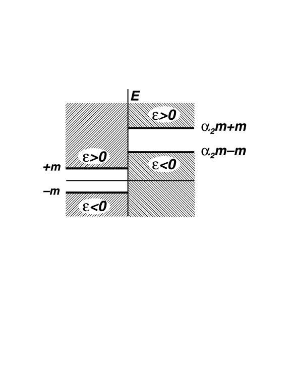
Figure 1: The interface between the vacuum (left-hand side of the picture) and the matter (right-hand side of the picture) with the corresponding neutrino band-gaps shown. The parameter $\alpha>2$.

Let us consider first a neutrino moving in the vacuum towards the interface with energy that falls into the band-gap region in matter. In this case the neutrino has no chance to survive in the matter and thus it is reflected from the interface. The same situation is realized for the antineutrino moving in the matter with energy falling into the band-gap in the vacuum. In this case the antineutrino is trapped by the matter. When the energies of neutrino in the vacuum or antineutrino in the medium fall into the region between the two band-gaps the effects of the neutrino-antineutrino annihilation or pair creation may occur (see, for example, the first paper of Ref. [10] and also [14, 15, 16]).

3.1 Majorana neutrino

We have considered so far the case of Dirac neutrino. Now let us turn to Majorana neutrino [37]. For a Majorana neutrino we derive the following contribution to the effective Lagrangian accounting for the interaction with the background medium

$$\Delta L_{eff}=-f^{\mu}(\bar{\nu}\gamma_{\mu}\gamma^{5}\nu),$$ (50)

which leads to the Dirac equation

$$\Big{\{}i\gamma_{\mu}\partial^{\mu}-\gamma_{\mu}\gamma_{5}f^{\mu}-m\Big{\}}\Psi(x)=0.$$ (51)

This equation differs from the one, obtained in the Dirac case, by doubling of the interaction term and lack of the vector part. The corresponding energy spectrum for the equation (51) is:

$$E_{\varepsilon}=\varepsilon{\sqrt{{\bf p}^{2}\Big{(}1-2s\alpha\frac{m}{p}\Big{)}^{2}+m^{2}}}.$$ (52)

From this expression it is clear, that the energy of the Majorana neutrino has its minimal value equal to the neutrino mass, $E=m$. This means that no effects are anticipated for the Majorana neutrino such as the Dirac neutrino has at the two media interface and which are discussed above. So that, in particular, there is no Majorana neutrino trapping and reflection by matter. It should be noted that the equation (51) and the Majorana neutrino spectrum in matter were discussed previously also in [10, 11].

3.2 Flavour neutrino energy difference in matter

Although the neutrino energy spectra corespondent to the modified Dirac-Pauli and Dirac equations are not the same, an equal result given by (24) for the energy difference $\Delta E=E(s=-1)-E(s=+1)$ of the two neutrino helicity states can be obtained from both of the spectra in the low matter density limit $\alpha\frac{pm}{E_{0}^{2}}\ll 1$.

It should be also noted that for the relativistic neutrinos the energy spectrum for the neutrino helicity states of Eq.(44) in the low density limit reproduces the correct energy values for the neutrino left-handed and right-handed chiral states:

$$E_{\nu_{L}}\approx E(s=-1)\approx E_{0}+{{\tilde{G}}_{F}\over\sqrt{2}}n,$$ (53)

and

$$E_{\nu_{R}}\approx E(s=-1)\approx E_{0},$$ (54)

as it should be for the active left-handed and sterile right-handed neutrino in matter.

We should like to note, that the obtained spectra for the flavor neutrinos of different helicities in the presence of matter enables one to reproduce the well-known result for the energy difference of two flavour neutrinos in matter. In order to demonstrate this we expand the expressions for the relativistic electron and muon neutrino energies, which are giving by (44) for the Dirac case or by (52) for the Majorana case, over $m/p\ll 1$ and get

$$E_{\nu_{e},\nu_{\mu}}^{s=-1}\approx E_{0}+2\alpha_{\nu_{e},\nu_{\mu}}m.$$ (55)

Then the energy difference for the two active flavour neutrinos will be

$$\Delta E=E_{\nu_{e}}^{s=-1}-E_{\nu_{\mu}}^{s=-1}=\sqrt{2}G_{F}n_{e}.$$ (56)

Analogously, considering the spin-flavour oscillations $\nu_{e_{L}}\rightleftarrows\nu_{\mu_{R}}$, for the corresponding energy difference we find:

$$\Delta E=E_{\nu_{e}}^{s=-1}-E_{\nu_{\mu}}^{s=+1}=\sqrt{2}G_{F}\big{(}n_{e}-{1\over 2}n_{n}\big{)}.$$ (57)

These equations enable one to get the expressions for the neutrino flavour and spin-flavour oscillation probabilities with resonance dependences on the matter density in the complete agreement with the results of [3, 4].

4 Neutrino spin light in matter

In this section we illustrate how the method based on the use of the exact solutions of the modified Dirac equation for the neutrino wave function can be used in the study of different phenomena which may exist when a neutrino moves in matter. We consider the spin light of neutrino ($SL\nu$), a new type of electromagnetic radiation that can be produced by the Dirac neutrino with nonzero magnetic moment while moving in the background matter. This phenomena was first predicted and studied within the quasi-classical theory in [32]. The $SL\nu$ is a quantum phenomenon by its nature, that is why it was important to elaborate the quantum treatment of this process [18, 19, 20].

The $SL\nu$ in matter originates from the quantum electromagnetic transition between the different helicity states due to the neutrino magnetic moment interactions with photons. In this section we give the quantum theory of the effect, that is based on the approach similar to the Furry representation in the quantum electrodynamics which has been discussed above in Introduction.

The corresponding Feynman diagram of the process under consideration is shown in Fig.2. The neutrino initial $\psi_{i}$ and final $\psi_{f}$ states are described by “broad lines” that account for the neutrino interaction with matter.

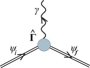
Figure 2: The $SL\nu$ radiation diagram.

The corresponding amplitude is given by

$$\begin{array}[]{c}\displaystyle S_{fi}=-\mu\sqrt{4\pi}\int d^{4}x{\bar{\psi}}_{f}(x)({\hat{\bf\Gamma}}{\bf e}^{*})\frac{e^{ikx}}{\sqrt{2\omega L^{3}}}\psi_{i}(x),\\ \\ \hat{\bf\Gamma}=i\omega\big{\{}\big{[}{\bf\Sigma}\times{\bm{\varkappa}}\big{]}+i\gamma^{5}{\bf\Sigma}\big{\}},\end{array}$$ (58)

where $\mu$ is the neutrino magnetic moment, $k^{\mu}=(\omega,{\bf k})$ and ${\bf e}^{*}$ are the photon momentum and polarization vectors, ${\bm{\varkappa}}={\bf k}/{\omega}$ is the unit vector pointing in the direction of the emitted photon propagation. Here again we consider the case of the electron neutrino moving in unpolarized matter composed of electrons. Then the integration over the time and spatial coordinates in (58) gives

$$S_{fi}=-\mu{\sqrt{\frac{2\pi}{\omega L^{3}}}}~{}2\pi\delta(E^{\prime}-E+\omega)\delta^{3}({\bf p^{\prime}}-{\bf p}+{\bf k}){\bar{u}}_{f}(E^{\prime},{\bf p^{\prime}})({\hat{\bf\Gamma}}{\bf e}^{*})u_{i}(E,{\bf p}).$$ (59)

The unprimed and primed symbols refer to initial and final neutrino states, respectively. From the energy-momentum conservation law

$$E=E^{\prime}+\omega,\ \ \ {\bf p}={\bf p}^{\prime}+{\bm{k}},$$ (60)

it follows that photon is radiated only when the initial and final neutrino states are characterized by $s_{i}=-1$ and $s_{f}=+1$, respectively. For the emitted photon energy we then obtain:

$$\omega=\frac{2\alpha mp\left[(E-\alpha m)-\left(p+\alpha m\right)\cos\theta\right]}{\left(E-\alpha m-p\cos\theta\right)^{2}-\left(\alpha m\right)^{2}},$$ (61)

where the angle $\theta$ gives the direction of the radiation in respect to the initial neutrino momentum $\bf p$. For the $SL\nu$ radiation rate and total power we get, respectively,

$$\Gamma=\mu^{2}\int_{0}^{\pi}\frac{\omega^{3}}{1+\tilde{\beta}^{\prime}y}S\sin\theta d\theta,\ \ \ I=\mu^{2}\int_{0}^{\pi}\frac{\omega^{4}}{1+\tilde{\beta}^{\prime}y}S\sin\theta d\theta,$$ (62)

where

$$S=(\tilde{\beta}\tilde{\beta}^{\prime}+1)(1-y\cos\theta)-(\tilde{\beta}+\tilde{\beta}^{\prime})(\cos\theta-y),$$ (63)

$$\tilde{\beta}=\frac{p+\alpha m}{E-\alpha m},\ \ \tilde{\beta}^{\prime}=\frac{p^{\prime}-\alpha m}{E^{\prime}-\alpha m},\ \ \ E^{\prime}=E-\omega,\ \ \ p^{\prime}=K\omega-p,$$ (64)

$$y=\frac{\omega-p\cos\theta}{p^{\prime}},\ \ K=\frac{E-\alpha m-p\cos\theta}{\alpha m}.$$ (65)

In the relativistic neutrino momentum case, $p\gg m$, and for different values of the matter density parameter $\alpha$ from (62) and we have the following limiting values [18, 19] (see also [20]):

$$\Gamma=\left\{\begin{tabular}[]{c}\ $\frac{64}{3}\mu^{2}\alpha^{3}p^{2}m,$\\ \ $4\mu^{2}\alpha^{2}m^{2}p$,\\ \ $4\mu^{2}\alpha^{3}m^{3}$,\end{tabular}\right.\ \ I=\left\{\begin{tabular}[]{cc}\ $\frac{128}{3}\mu^{2}\alpha^{4}p^{4},$&\ \ \ for {$\alpha\ll\frac{m}{p},$}\\ \ $\frac{4}{3}\mu^{2}\alpha^{2}m^{2}p^{2}$,&\ \ \ \ \ \ \ \ { for $\frac{m}{p}\ll\alpha\ll\frac{p}{m},$}\\ \ $4\mu^{2}\alpha^{4}m^{4}$,&\ { for $\alpha\gg\frac{p}{m}.$}\end{tabular}\right.$$ (66)

In the opposite case of “non-relativistic” neutrinos, $p\ll m$, we get:

$$\Gamma=\left\{\begin{tabular}[]{c}\ $\frac{64}{3}\mu^{2}\alpha^{3}p^{3},$\\ \ $\frac{512}{5}\mu^{2}\alpha^{6}p^{3}$,\\ \ $4\mu^{2}\alpha^{3}m^{3}$,\end{tabular}\ \ \ I=\left\{\begin{tabular}[]{cc}\ $\frac{128}{3}\mu^{2}\alpha^{4}p^{4},$&\ \ \ \ \ for {$\alpha\ll 1,$}\\ \ $\frac{1024}{3}\mu^{2}\alpha^{8}p^{4}$,&\ \ \ \ \ \ \ \ \ \ { for $1\ll\alpha\ll\frac{m}{p},$}\\ \ $4\mu^{2}\alpha^{4}m^{4}$,&\ \ \ \ { for $\alpha\gg\frac{m}{p}.$}\end{tabular}\right.\right.$$ (67)

It can be seen that in the case of a very dense matter the values of the rate and total power are mainly determined by the density. Note that the obtained above results in the case of small densities are in agreement with the studies of the neutrino spin light performed on the basis of the quasi-classical approach [32]. The $SL\nu$ characteristics in the case of matter with “moderate”  densities ( the second lines of (66) ) were also obtained in [40].

One can estimate the average emitted photon energy $\left\langle\omega\right\rangle={I}/{\Gamma}$ with the use of the obtained above values of the rate and total power (66) and (67) for different matter densities. In the two case ($p\gg m$ and $p\ll m$), we get, respectively,

$$\left\langle\omega\right\rangle\simeq\left\{\begin{tabular}[]{cc}\ $2\alpha\frac{p^{2}}{m},$&for {$\alpha\ll\frac{m}{p},$}\\ \ $\frac{1}{3}p$,&{ for $\frac{m}{p}\ll\alpha\ll\frac{p}{m},$}\\ \ $\alpha m$,&\ { for $\alpha\gg\frac{p}{m}$},\end{tabular}\right.\left\langle\omega\right\rangle\simeq\left\{\begin{tabular}[]{cc}\ $2\alpha p,$&for {$\alpha\ll 1,$}\\ \ $\frac{10}{3}\alpha^{2}p$,&{ for $1\ll\alpha\ll\frac{m}{p},$}\\ \ $\alpha m$,&{ for $\alpha\gg\frac{m}{p}.$}\end{tabular}\right.$$ (68)

To summaries the main properties of the spin light of neutrino in matter, we should like to point out that this phenomenon arises due to neutrino energy dependence in matter on the neutrino helicity state. In media characterized by the positive values of the parameter $\alpha$, the negative-helicity neutrinos (the left-chiral relativistic neutrinos) are converted into the positive-helicity neutrinos (the right-chiral relativistic neutrinos) in the process under consideration. Thus, the neutrino self-polarization effect can appear (see also [32]). From the above estimations for the emitted photon energies it follows that for the ultra-relativistic neutrinos moving in dense matter the $SL\nu$ can be regarded as an effective mechanism for production of the gamma-rays.

Note that an adequate description of the $SL\nu$ in the low matter density limit $\alpha\frac{pm}{E_{0}^{2}}\ll 1$ can be obtained on the basis of the Dirac-Pauli equation for the neutrino wave function [35]. More over, the use of the Dirac-Pauli equation enables us also to consider the $SL\nu$ in the case of totally polarized (due to the presence of strong magnetic field with the strength given by (31) ) electron gas. For this particular situation, the emitted $SL\nu$ photon energy, as it follows from (33), is given by

$$\omega=\frac{\beta}{1-\beta_{e}\cos\theta}\omega_{0},$$ (69)

where

$$\omega_{0}=\frac{{G}_{F}}{\sqrt{2}}n\left[\left(1+\sin^{2}4\theta_{W}\right)-{sign\left(\frac{B_{\parallel}}{B}\right)}\right]+2\frac{\mu B_{\parallel}}{\gamma}.$$ (70)

A remark on the possibility for Majorana neutrino to emit the spin light in matter should be made. Obviously, due to the absence of the magnetic moment, such radiation is not expected in this case. However, having two neutrinos of different flavour, it is possible to produce an analogous effect via the transition magnetic moment, which Majorana neutrinos can possess.

5 Modified Dirac equation for electron in matter

In [20, 21], it has been shown how the approach, developed at first for description of a neutrino motion in the background matter, can be spread for the case of an electron propagating in matter. The modified Dirac equation for an electron in matter has been derived [20] and on this basis we have considered the electromagnetic radiation that can be emitted by the electron (due to its electric charge) in the background matter. We have termed this radiation as the  “spin light of electron” in matter. It should be noted here that the term  “spin light” was introduced in [41] for designation of the particular spin-dependent contribution to the electron synchrotron radiation power.

Let us consider an electron having the standard model interactions with particles of electrically neutral matter composed of neutrons, electrons and protons. This can be used for modelling a real situation existed, for instance, when electrons move in different astrophysical environments. We suppose that there is a macroscopic amount of the background particles in the scale of an electron de Broglie wave length. In fact, we account below only the neutron component of matter. Then the addition to the electron effective interaction Lagrangian is

$$\Delta L^{(e)}_{eff}=-{f}^{\mu}\Big{(}\bar{e}\gamma_{\mu}{1-4\sin^{2}\theta_{W}+\gamma^{5}\over 2}e\Big{)},$$ (71)

where the explicit form of $f^{\mu}$ depends on the background particles density, speed and polarization and is determined by (34) and (35). The modified Dirac equation for the electron wave function in matter is [20]

$$\Big{\{}i\gamma_{\mu}\partial^{\mu}-\frac{1}{2}\gamma_{\mu}(1-4\sin^{2}\theta_{W}+\gamma_{5}){\widetilde{f}}^{\mu}-m_{e}\Big{\}}\Psi_{e}(x)=0,$$ (72)

where for the case of electron moving in the background of neutrons (that can be used as an abrupt model of a nuclear matter of a neutron star, see, for instance, [16])

$${\tilde{f}}^{\mu}=-f^{\mu}=\frac{G_{F}}{\sqrt{2}}(j^{\mu}_{n}-\lambda^{\mu}_{n}).$$ (73)

We consider below unpolarized neutrons so that

$$\widetilde{f}^{\mu}=\frac{G_{F}}{\sqrt{2}}(n_{n},n_{n}{\bf v}),$$ (74)

here $n_{n}$ is the neutrons number density and $\mathbf{v}$ is the speed of the reference frame in which the mean momentum of the neutrons is zero.

The corresponding electron energy spectrum in the case of unpolarized matter at rest is given by

$$E_{\varepsilon}^{(e)}=\varepsilon\sqrt{{{\bf p}_{e}}^{2}\Big{(}1-s_{e}\alpha_{n}\frac{m_{e}}{p_{e}}\Big{)}^{2}+{m_{e}}^{2}}+c{\alpha}_{n}m_{e},\ \ \alpha_{n}=\frac{1}{2\sqrt{2}}{G_{F}}\frac{n_{n}}{m_{e}},$$ (75)

where $c=1-4\sin^{2}\theta_{W}$ and the notations for the electron mass, momentum, helicity and sign of energy are similar to those used in Section 2 for the case of neutrino. For the wave function of the electron moving in nuclear matter we get [21]

$$\Psi_{\varepsilon,{\bf p},s}({\bf r},t)=\frac{e^{-i(E^{(e)}_{\varepsilon}t-{\bf p}{\bf r})}}{2L^{\frac{3}{2}}}\left(\begin{array}[]{c}{\sqrt{1+\frac{m_{e}}{E^{(e)}_{\varepsilon}-c\alpha_{n}m_{e}}}}\ \sqrt{1+s\frac{p_{3}}{p}}\\ {s\sqrt{1+\frac{m_{e}}{E^{(e)}_{\varepsilon}-c\alpha_{n}m_{e}}}}\ \sqrt{1-s\frac{p_{3}}{p}}\ \ e^{i\delta}\\ {s\varepsilon\sqrt{1-\frac{m_{e}}{E^{(e)}_{\varepsilon}-c\alpha_{n}m_{e}}}}\ \sqrt{1+s\frac{p_{3}}{p}}\\ {\varepsilon\sqrt{1-\frac{m_{e}}{E^{(e)}_{\varepsilon}-c\alpha_{n}m_{e}}}}\ \ \sqrt{1-s\frac{p_{3}}{p}}\ e^{i\delta}\end{array}\right)$$ (76)

The exact solutions of this equation open a new method for investigation of different quantum processes which can appear when electrons propagate in matter. On this basis, we predict and investigate the $SLe$ [20, 21]. The $SLe$ photon energy, obtained from the energy conservation law, is given by

$$\omega_{SLe}=\frac{2\alpha_{n}m_{e}p_{e}\left[(E^{(e)}-c\alpha_{n}m_{e})-\left(p_{e}+\alpha_{n}m_{e}\right)\cos\theta_{SLe}\right]}{\left(E^{(e)}-c\alpha_{n}m_{e}-p_{e}\cos\theta_{SLe}\right)^{2}-\left(\alpha_{n}m_{e}\right)^{2}},$$ (77)

where the angle $\theta_{SLe}$ gives the direction of the radiation in respect to the initial electron momentum ${\bf p}_{e}$. In the case of relativistic electrons and small values of the matter density parameter $\alpha_{n}$ the photon energy is

$$\omega_{SLe}=\frac{\beta_{e}}{1-\beta_{e}\cos\theta_{SLe}}\omega_{0},\ \ \ \omega_{0}=\frac{G_{F}}{\sqrt{2}}n_{n},$$ (78)

here $\beta_{e}$ is the electron speed in vacuum. From this expressions we conclude that for the relativistic electrons the energy range of the $SLe$ may even extend up to energies peculiar to the spectrum of gamma-rays. We also predict the existence of the electron-spin polarization effect in this process. Finally, from the order-of-magnitude estimation, we expect that the ratio of rates of the $SLe$ and the $SL\nu$ in matter is

$$R=\frac{\Gamma_{SLe}}{\Gamma_{SL\nu}}\sim\frac{e^{2}}{\omega^{2}\mu^{2}},$$ (79)

that gives $R\sim 10^{18}$ for the radiation in the range of gamma-rays, $\omega\sim 5\ MeV$, and for the neutrino magnetic moment $\mu\sim 10^{-10}\mu_{0}$. Thus, we expect that in certain cases the $SLe$ in matter would be more effective than the $SL\nu$.

6 Conclusion

In this paper, we have developed a framework for treating different interactions of neutrinos and electrons in the presence of matter. This method is based on the use of modified Dirac equations for particles wave functions, in which the correspondent effective potentials that account for the interaction with matter are included.

For a neutrino moving in matter, we have considered the modified Dirac-Pauli and Dirac equations and evaluated the correspondent wave functions and energy spectra in the presence of matter. Both cases of Dirac and Majorana neutrinos have been discussed.

Within the framework developed, we have also derived the modified Dirac equation for the electron moving in matter and evaluated the exact wave functions and energy spectra.

The approach developed is similar to the Furry representation which is used in quantum electrodynamics in investigations of particles interactions in the presence of external electromagnetic fields. Note that our focus has been on the standard model interactions of neutrinos and electrons with the background matter. The same approach, which implies the use of the exact solutions of the correspondent modified Dirac equations, can be used in the case when neutrinos and electrons interact with different external fields predicted within extensions of the standard model (see, for instance, [25, 26]).

In conclusion, we should like to note that the approach developed is valid in the case when the interaction of neutrinos and electrons with particle of the background is coherent. This condition is satisfied when a macroscopic amount of the background particles are confined within the scale of a neutrino or electron de Broglie wave length. So that for the relativistic neutrinos and electrons $(l=\nu$ or $e)$ the following condition must be satisfied

$$\frac{n}{\gamma_{l}m^{3}_{l}}\gg 1,$$ (80)

where $n$ is the number density of matter and $\gamma_{l}=\frac{E_{l}}{m_{l}}$. For instance, let us consider the case of neutrino. If we express $n$ by the dimensional number $N$ following to $n=N\ cm^{-3}=N\times 2^{3}\times 10^{-15}eV^{3}$ and for the neutrino mass use the value of $m_{\nu}\sim 1\ eV$, then from (80) we have

$$N\gg 10^{14}\times\Big{(}\frac{E_{\nu}}{1\ eV}\Big{)}.$$ (81)

It follows that even for not extremely dense astrophysical matter with $N\sim 10^{33}$ (this value is about five orders of magnitude lower then one peculiar to densities of neutron stars) the approach developed is valid for the neutrino ultra-high energy band.

References

- [1] W.Pauli, On the earlier and more recent history of the neutrino, in: “Neutrino physics”, ed. by K.Winter, Cambridge University Press, 1991.
- [2] R.Mohapatra, A.Smirnov, Ann.Rev.Nucl.Part.Phys.56 (2006), at press.
- [3] L.Wolfenstein, Phys.Rev.D 17 (1978) 2369; S.Mikheyev, A.Smirnov, Sov.J.Nucl.Phys.42 (1985) 913.
- [4] E.Akhmedov, Phys.Lett.B 213 (1988) 64; C.-S.Lim, W.Marciano, Phys.Rev.D37 (1988) 1368.
- [5] G.Raffelt,“Stars as Laboratories for Fundamental Physics”, The University of Chicago Press, 1995.
- [6] P.Mannheim Phys.Rev.D37 (1988) 1935.
- [7] D.Nötzold, G.Raffelt, Nucl.Phys.B307 (1988) 924.
- [8] J.Nieves, Phys.Rev.D40 (1989) 866.
- [9] L.N. Chang and R.K.Zia, Phys.Rev.D38 (1988) 1669.
- [10] J.Pantaleone, Phys.Lett.B268 (1991) 227; Phys.Rev.D46 (1992) 510; K.Kiers, N.Weiss, Phys.Rev.56 (1997) 5776; K.Kiers, M.Tytgat, Phys.Rev.D57 (1998) 5970.
- [11] Z.Berezhiani, M.Vysotsky, Phys.Lett.B 199 (1987) 281; Z.Berezhiani, A.Smirnov, Phys.Lett.B 220 (1989) 279.; C.Giunti, C.W.Kim, U.W.Lee, W.P.Lam, Phys.Rev.D 45 (1992) 1557; Z.Berezhiani, A.Rossi, Phys.Lett.B336 (1994) 439.
- [12] V.Oraevsky, V.Semikoz, Ya.Smorodinsky Phys.Lett.B227 (1989) 255.
- [13] W.Haxton, W.-M.Zhang, Phys.Rev.D43 (1991) 2484.
- [14] A.Loeb Phys.Rev.Lett.64 (1990) 115.
- [15] M.Kachelriess, Phys.Lett.B426 (1998) 89.
- [16] A.Kusenko, M.Postma, Phys.Lett.B 545 (2002) 238.
- [17] H.B.J.Koers, hep-ph/0409259.
- [18] A.Studenikin, A.Ternov, Phys.Lett.B 608 (2005) 107, hep-ph/041097, hep-ph/041096, hep-ph/0412408.
- [19] A.Grigoriev, A.Studenikin, A.Ternov, Phys.Lett.B 622 (2005) 199; Grav.Cosmol. 11 (2005) 132, hep-ph/0502231.
- [20] A.Studenikin, J.Phys.A: Math. Gen. 39 (2006) 6769; hep-ph/0511311; presented at 7th Int.Workshop on QuantumField Theory under the Influence of External Conditions (QFEXT’05, Barcelona, Spain, September 2005) and at 22nd Int.Conf. on Neutrino Physics and Astrophysics (Santa Fe, New Mexico, June 13-19, 2006).
- [21] A.Grigoriev, S.Shinkevich, A.Studenikin, A.Ternov, I.Trofimov, in: “Particle Physics at the Year of the 250th Anniversary of Moscow University”, ed. by A.Studenikin, World Scientific (Singapore), 2006, p. 73.
- [22] W.Furry, Phys.Rev. 81 (1951) 115.
- [23] N.N.Bogoliubov, D.V.Shirkov, “Introduction to the theory of quantized fields”, John Willey & Sons, Inc., New York, 3rd edition, 1980.
- [24] A.A.Sokolov, I.M.Ternov, “Synchrotron radiation”, Pergamon press, Oxford, 1968.
- [25] D.Colladay, V.A.Kostelecky, Phys.Rev.D 55 (1997) 6760.
- [26] V.Ch.Zhukovsky, A.E.Lobanov, E.M.Murchikova, Phys.Rev.D 73 (2006) 065016.
- [27] K.Fujikawa, R.Shrock, Phys.Rev.Lett.45 (1980) 963.
- [28] A.Borisov, V.Zhukovsky, A.Ternov, Sov.Phys.J. 31 (1988) 228.
- [29] M.Dvornikov, A.Studenikin, Phys.Rev.D 69 (2004) 073001; JETP 99 (2004) 254.
- [30] A.Egorov, A.Lobanov, A.Studenikin, Phys.Lett.B491 (2000) 137; A.Lobanov, A.Studenikin, Phys.Lett.B515 (2001) 94.
- [31] M.Dvornikov, A.Studenikin, JHEP 09 (2002) 016.
- [32] A.Lobanov, A.Studenikin, Phys.Lett.B564 (2003) 27; A.Lobanov, A.Studenikin, Phys.Lett.B 601 (2004) 171; M.Dvornikov, A.Grigoriev, A.Studenikin, Int.J.Mod.Phys.D 14 (2005) 309.
- [33] A.Studenikin, Phys.Atom.Nucl. 67 (2004) 993.
- [34] V.Bargmann, L.Michel, V.Telegdi, Phys.Rev.Lett. 2 (1959) 435.
- [35] A.Grigoriev, A.Studenikin, A.Ternov, in: A.Studenikin (Ed.), “Particle Physics in Laboratory, Space and Universe”, World Scientific (Singapore) p. 55 (2005), hep-ph/0502210.
- [36] H.Nunokawa, V.Semikoz, A.Smirnov, J.Valle, Nucl.Phys.B501, 17 (1997).
- [37] A.Grigoriev, A.Studenikin, A.Ternov Phys.Atom.Nucl.69 (2006) 1940.
- [38] I.Pivovarov, A.Studenikin, PoS(HEP2005) (2006) 191; hep-ph/0512031.
- [39] A.Grigoriev, A.Studenikin, A.Ternov, Phys.Lett.B 622 (2005) 199.
- [40] A.Lobanov, Phys.Lett.B 619 (2005) 136; Dokl.Phys. 50 (2005) 286.
- [41] I.M.Ternov, Sov.Phys.Usp. 38 (1995) 405; V.A.Bordovitsyn, I.M.Ternov, V.G.Bagrov, Sov.Phys.Usp. 38 (1995) 1037.