ROM2F/2006/24

Deflected Anomaly Mediation and Neutralino Dark Matter
Alessandro Cesarini, Francesco Fucito and Andrea Lionetto
Dipartimento di Fisica, Università di Roma “Tor Vergata”
I.N.F.N. Sezione di Roma II,
Via della Ricerca Scientifica, 00133 Roma, Italy

Abstract

This is a study of the phenomenology of the neutralino dark matter in the so called deflected anomaly mediation scenario. This scheme is obtained from the minimal anomaly mediated scenario by introducing a gauge mediated sector with $N_{f}$ messenger fields. Unlike the former scheme the latter has no tachyons. We find that the neutralino is still the LSP in a wide region of the parameter space: it is essentially a pure bino in the scenario with $N_{f}=1$ while it can also be a pure higgsino for $N_{f}>1$. This is very different from the naive anomaly mediated scenario which predicts a wino like neutralino. Moreover we do not find any tachyonic scalars in this scheme. After computing the relic density (considering all the possible coannihilations) we find that there are regions in the parameter space with values compatible with the latest WMAP results with no need to consider moduli fields that decay in the early universe.

1 Introduction

Dark matter still remains one of the main unsolved problem in physics. The common accepted paradigm is the existence of an exotic weakly interacting massive particle (WIMP). Such a particle has to be found in some extension of the Standard Model (SM) of particle physics. It is well known that supersymmetry is an essential ingredient of a consistent theory beyond the SM and the most studied framework is the MSSM, the minimal supersymmetric extension of the SM. In the MSSM the lightest supersymmetric particle (LSP) is usually a neutralino, which is a good candidate for cold dark matter [1]. The pattern of the soft supersymmetry breaking terms greatly affects the composition and the strength of the dominant interactions of the neutralino. Hence it is very interesting to study the neutralino phenomenology in different supersymmetry breaking scenarios. It is in general very difficult to find a mechanism which is able to generate a suitable soft supersymmetry breaking lagrangian without the need of any fine-tuning. There are essentially three main classes of possible mechanisms which are differentiated by the vehicle which transmits the supersymmetry breaking from the primary “source” to the MSSM fields. The first and most studied scenario is gravity mediation [4] in which the supersymmetry breaking is vehicled by tree-level Planck suppressed couplings. Another widely studied scenario is gauge mediation (GMSB) [5] in which ordinary gauge interactions vehicle the breaking. The last scenario is anomaly mediation (AMSB) [6] in which supersymmetry breaking is transmitted to the MSSM due to the $R$-symmetry and scale anomalies. Although very natural, the gravity-mediated schemes have the unwanted feature that in order to be phenomenologically viable they must suppose fine-tuned forms for the superpotential and Kähler potential [6]. On the other hand the gauge-mediated scheme does not have such problem, but it predicts the gravitino as the LSP, which is not the most suitable candidate to constitute dark matter.

The anomaly-mediated models do not have any of the last two undesirable features, since they usually predict the neutralino to be the LSP and any direct gravitational coupling between the primary supersymmetry breaking source and the MSSM to be suppressed. Anyway the minimal AMSB (mAMSB) scheme predicts some MSSM scalars to be tachyonic and hence there must be some other mechanism to lift their squared masses to positive values. In this paper we consider AMSB models with an additional GMSB-like contribution to the soft terms which makes them tachyon free. Such scheme is called deflected anomaly mediated (dAMSB) [12, 13]. The plan of the paper is as follows: in the second section we give a brief introduction to the minimal anomaly mediated scenario while in the third section we describe the deflected anomaly mediated scenario. In the fourth section we show what kind of supersymmetry breaking terms arise from deflected anomaly mediation leaving to the appendix all the details of the computation. In the fifth section we present the phenomenological implications for dark matter. The last section is devoted to the conclusions.

2 Anomaly Mediation Revisited

We consider an expansion of the $D=4$ supergravity action in inverse powers of the Planck mass ($M_{P}\simeq 1.2\times 10^{19}$ GeV). We are only interested in terms that have no Planck suppression and that involve only the vierbein and the complex scalar auxiliary field $M$ of the supergravity multiplet, besides the terms which do not contain any supergravity fields at all. The lagrangian [6] can be written as:

$$\frac{L}{e} = \left[f(Q^{\dagger},e^{-V}Q)\varphi^{\dagger}\varphi\right]_{\theta^{2}{\bar{\theta}}^{2}}+$$ (2.1)

$$\left[\left(\varphi^{3}W(Q)+\tau_{ab}\left(Q\right){{\cal W}^{a}}{{\cal W}^{b}}\right)_{\theta^{2}}+h.c.\right]+$$

$$+\frac{1}{6}f(Q^{\dagger},e^{-V}Q){\cal{R}}+\left\{\mbox{$b_{a}$ and $\psi_{m}^{\;\;\alpha}$ terms}\right\}+{{\cal{O}}\left(M_{P}^{-1}\right)}$$

where the $Q$’s are the chiral matter superfields, $\cal{W}$ is the chiral gauge field strength, $b_{a}$ and $\psi_{m}^{\;\;\alpha}$ are respectively the vector auxiliary field and the gravitino field while $e$ is the vierbein determinant. The real function $f$ gives the kinetic term for the $Q$’s superfield while the $\tau$ function gives the normalization for the gauge term. We assume for $\tau$ the minimal form, i.e. $\tau_{ab}\propto\delta_{ab}$.

The lagrangian in eq. (2.1) is written in the flat space superfield notation [8], and the spurion chiral superfield $\varphi$ is taken to be

$$\varphi=1-\frac{M^{*}}{3}\theta^{2}=1+F_{\varphi}\theta^{2}.$$ (2.2)

By expanding the function $f$ in powers of $M_{P}$, and modulo a rigid rescaling of the $Q$ superfields, we can write:

$$f(Q^{\dagger},e^{-V}Q)=-3M_{P}^{2}+Q^{\dagger}e^{-V}Q+{{\cal{O}}\left(M_{P}^{-1}\right)}.$$ (2.3)

Inserting this last equation into eq. (2.1) and dropping all the scalar curvature, auxiliary vector and gravitino terms we get

$$\frac{L}{e}=\left[Q^{\dagger}e^{-V}Q\varphi^{\dagger}\varphi\right]_{\theta^{2}{\bar{\theta}}^{2}}+\left[\left(\varphi^{3}W(Q)+\tau\left(Q\right){\cal{W}}{\cal{W}}\right)_{\theta^{2}}+h.c.\right],$$ (2.4)

This action takes into account the couplings of the matter superfields to the complex scalar auxiliary field $M$ of the minimal supergravity multiplet, which could acquire a nonzero vev in case of supersymmetry breaking. The lagrangian ${\cal L}$ of eq. (2.4) can be thought of as the effective lagrangian in the flat space limit substituting $M$ with its supersymmetry breaking vev, $M\rightarrow\left<M\right>$, and the vierbein determinant with its flat space value, $e\rightarrow 1$. In this way, we have a theory which is manifestly invariant under supersymmetry transformations (being written in superspace notation) and in which supersymmetry turns out to be gauge fixed by the condition on the $\varphi$ superfield derived from (2.2). This is the mechanism able to transmit the supersymmetry breaking to the $Q$ superfields, which will be finally identified with the MSSM superfields (on the visible brane). An important remark is that if the superpotential $Q$ had no explicit mass scale, i.e. $W\sim Q^{3}$, the $\varphi$ dependence in eq. (2.4) could be immediately eliminated through a superfield rescaling:

$$Q\varphi\rightarrow Q.$$ (2.5)

In this case there would be no tree level communication of the supersymmetry breaking. However the situation is different at the one loop level because the $\varphi$ superfield cannot be eliminated through the rescaling (2.5). To see how the mechanism works let us start from the action corresponding to eq. (2.4) with $W=y_{0}Q^{3}$:

$$S=\int d^{4}x\left\{\left[Q^{\dagger}e^{-V}Q\varphi^{\dagger}\varphi\right]_{\theta^{2}{\bar{\theta}}^{2}}+\left[\left(y_{0}Q^{3}\varphi^{3}+\tau\left(Q\right){\cal{W}}{\cal{W}}\right)_{\theta^{2}}+h.c.\right]\right\},$$ (2.6)

where $y_{0}$ is a dimensionless parameter. The classical scale invariance of the action $S$ can be inferred from the absence of explicit mass parameters. The action $S$ is also classically invariant under the $R$-symmetry, provided that one assigns suitable $R$-weights to the $Q$ and $\varphi$ superfields. The action of the $R$-symmetry on a chiral superfield $\Phi=\left(A,\psi,F\right)$ of $R$-weight $w_{\Phi}$ is defined by

$$A \to A^{\prime}=e^{2iw_{\Phi}\lambda}A$$

$$\psi \to \psi^{\prime}=e^{2i(w_{\Phi}-1)\lambda}\psi$$ (2.7)

$$F \to F^{\prime}=e^{2i(w_{\Phi}-2)\lambda}F$$

for real $\lambda$. The kinetic term in eq. (2.6) is $R$-invariant independently of the $R$-weights of $Q$ and $\Phi$, while the superpotential is invariant if one assigns $w_{\varphi}=2/3$ and $w_{Q}=0$. With this assignment the gauge kinetic term has $w=2$ provided that $w_{Q}=0$ and hence it is classically $R$-invariant.

In order to cancel the ultraviolet divergences, it is necessary to add counterterms, that introduce at least one explicit mass parameter: the ultraviolet cutoff scale $\Lambda_{UV}$ of the theory. This scale appears also considering the theory as an effective one.

The generic form of the action remains that of eq. (2.6). It has a kinetic term and a superpotential term with the same $\varphi^{\dagger}\varphi$ and $\varphi^{3}$ couplings with the auxiliary field of the supergravity multiplet. In addition to the terms in eq. (2.6) the new kinetic and superpotential terms contain new regulating pieces in which the $\Lambda_{UV}$ dependence is explicit. The scale invariance of the theory is now lost due to the presence of a dimensionful parameter ($\Lambda_{UV}$), while the $R$-symmetry is preserved because it is determined by $\varphi$ (the only field with nonzero $R$-weight) which couples to the kinetic and superpotential terms in the same way as at tree level. It can be seen [6] that after the rescaling of the superfield of eq. (2.5) the $\varphi$ dependence does not disappear from the lagrangian unlike in the tree level case. The field $\varphi$ appears together with the explicit cutoff scale $\Lambda_{UV}$:

$$\Lambda_{UV}\rightarrow\varphi\Lambda_{UV}\quad\mbox{ or }\quad\Lambda_{UV}\rightarrow\varphi^{\dagger}\Lambda_{UV}.$$ (2.8)

Under the rescaling (2.5), both $Q$ and $\varphi$ acquire an $R$-weight equal to $2/3$ and, at the loop level, the lagrangian obeys the $R$-symmetry. Introducing the wave function renormalization for the chiral and gauge superfields the lagrangian becomes:

$$L=\left[Z_{Q}\left(\frac{\mu}{\Lambda_{UV}|\varphi|}\right)Q^{\dagger}e^{-V}Q\right]_{\theta^{2}{\bar{\theta}}^{2}}+$$

$$+\left\{\left[y_{0}Q^{3}+\tau\left(\frac{\mu}{\Lambda_{UV}\varphi}\right){\cal{W}}{\cal{W}}\right]_{\theta^{2}}+h.c.\right\}.$$ (2.9)

If we turn off the coupling to gravity, i.e. we fix $\varphi=1$, the $R$-symmetry is lost. This is a consequence of the fact that without the coupling to $\varphi$ the $R$-symmetry is anomalous. In this way we have shown that the $\varphi$ field cannot be decoupled from the loop level lagrangian through the rescaling of eq. (2.5) as in the case of the tree level lagrangian which does not contain explicit mass parameters. This implies that the supersymmetry breaking effects, which are encoded in the nonzero vev of the $\theta^{2}$ component of $\varphi$, are always transmitted at loop level to the matter and gauge superfields.

3 Deflected Anomaly

In its minimal form the anomaly mediated scenario [6] leads to tachyonic masses for the sleptons (which do not transform under the $SU(3)$ gauge group). Many different solutions to this problem has been proposed [14, 15, 16, 17, 18, 19, 20, 21, 22, 23, 24] but one of the most interesting and elegant relies in considering an additional gauge mediated sector. By introducing $N_{f}$ messengers fields the RGE gets modified in such a way to avoid tachyons at the weak scale.

One of the prediction of the deflected anomaly models is the non universality of the gaugino masses at the GUT scale (even at the messenger scale).

Let us start from the anomaly mediated sector. We assume the setup of [9, 10, 11] with two branes in a $D=5$ space-time where the $5^{\rm th}$ component is compactified over the orbifold $S^{1}/Z^{2}$. The hidden brane is the source of the breaking of supersymmetry through the (super)conformal anomaly. Such geometrical setup permits to avoid any non gravitational coupling between the fields of the AMSB hidden sector (let us denote them by $\Sigma$) and those of the MSSM (let us denote them by $Q$). Such couplings could lead to phenomenologically dangerous flavor and CP violating effects. Their absence is due to a suppression factor, given by the bulk separation, which multiplies any non gravitational interaction term between an hidden sector superfield and a visible one. Such factors are absent for couplings which arise in a four dimensional space-time.

For example, a Kähler potential defined on the hidden brane

$$\frac{1}{M^{2}}\Sigma^{\dagger}\Sigma Q^{\dagger}Q$$ (3.10)

is gravitationally rescaled (actually this is a gravitational redshift) as

$$\frac{1}{M^{2}}\Sigma^{\dagger}\Sigma Q^{\dagger}Qe^{-m_{B}/\mu_{c}},$$ (3.11)

where $m_{B}$ is the mass of the non gravitational bulk state that vehicles the interaction across the bulk. The exponential suppression factor eliminates all the phenomenologically dangerous couplings of the form of eq. (3.11), once one assumes that every non gravitational bulk state has a mass quite larger than the compactification scale $\mu_{c}$. We do not need to know the detailed dynamic of the AMSB hidden sector except that the complex auxiliary field $M$ of the four-dimensional supergravity multiplet must acquire a vev $\left<M\right>$ in order to break supersymmetry on the visible brane. Now let us take into account the presence of an extra gauge mediated sector on the visible brane. We assume that in this sector there is a gauge singlet chiral superfield $X=\left(A_{X},\Psi_{X},F_{X}\right)$ which is directly coupled to $N_{f}$ copies of messenger chiral superfields $\Phi_{i}$ and ${\bar{\Phi}}_{i}$, transforming under the fundamentals and anti-fundamentals of the standard MSSM gauge groups. The tree level lagrangian for the $X$ superfield, in a $M_{P}^{-1}$ expansion, is of the same kind of the one in eq. (2.4), without the gauge kinetic part and with the substitution $Q\rightarrow X$. We can write:

$$L_{X}=\left[X^{\dagger}X\varphi^{\dagger}\varphi\right]_{\theta^{2}{\bar{\theta}}^{2}}+\left\{\left[\left(\lambda_{ij}\bar{\Phi}_{i}X\Phi_{j}+W\left(X\right)\right)\varphi^{3}\right]_{\theta^{2}}+h.c.\right\},$$ (3.12)

where we explicitly separate the part of the superpotential that involves only the messenger superfields, from the part that depends only on $X$. The coupling of the $X$ superfield to $\varphi$ ensures that the GSMB hidden sector is gravitationally coupled to the supersymmetry breaking source $\left<M\right>$. At this stage supersymmetry breaking can be transmitted to the GMSB hidden sector at tree level or at one loop level. The former case corresponds, as it was outlined in section 2, to a superpotential $W\left(X\right)$ that contains explicit mass scales [12], while the latter implies $W\left(X\right)\sim X^{3}$ or zero [13].

In this paper we consider a very general scenario in which the superpotential of the gauge hidden sector $W\left(X\right)$ contains all the terms with couplings of positive or vanishing mass dimension:

$$W\left(X\right)=c_{1}X^{3}+c_{2}\left<F_{\varphi}\right>X^{2}+c_{3}\left<F_{\varphi}\right>^{2}X+c_{4}\left<F_{\varphi}\right>^{3},$$ (3.13)

where the $c_{i}$ ($i=1,\cdots,4$) are real numbers and $\left<F_{\varphi}\right>=-\left<M^{*}\right>/3$. We also assume, without loss of generality, $\left<F_{\varphi}\right>$ to be real. In fact this condition could always be satisfied modulo a rigid rotation of the supergravity auxiliary field $M$.

As in the usual gauge mediation the messenger superfields $\Phi_{i}$ and $\bar{\Phi}_{i}$ acquire masses of order $\left<A_{X}\right>$ and a mass splitting of order $\sqrt{\left<F_{X}\right>}$ where $\left<A_{X}\right>$ and $\left<F_{X}\right>$ are respectively the vevs of the scalar and auxiliary part of the $X$ superfield. It is exactly the presence of an intermediate threshold given by the $X$ superfield vev which changes the renormalization group equations of the soft terms off the AMSB trajectory. In this way the negative squared masses are no longer present in the spectrum. The main source of supersymmetry breaking is the $\varphi$ superfield We choose the form of the superpotential in such a way to get the right vev for the $X$ superfield. In this way, besides a source of susy breaking for the AMSB we also have a similar one for the GMSB.

Upon substituting $\varphi=1+F_{\varphi}\theta^{2}$ into (3.12) and dropping all the terms involving the messenger superfields we have

$$L_{X} = \left(F_{\varphi}^{2}A_{X}A_{X}^{*}+F_{X}F_{X}^{*}-\partial_{\mu}A_{X}^{*}\partial^{\mu}A_{X}-i{\bar{\psi}}_{X}{\bar{\sigma}}^{\mu}\partial_{\mu}\psi_{X}\right)+$$ (3.14)

$$+A_{X}F_{X}^{*}F_{\varphi}+3W(A_{X})F_{\varphi}+F_{X}\frac{\partial W(A_{X})}{\partial A_{X}}+$$

$$-\frac{1}{2}\psi_{X}\psi_{X}\frac{\partial^{2}W(A_{X})}{\partial^{2}A_{X}}+h.c.,$$

where from now on, for the sake of simplicity, $F_{\varphi}$ stands for $\left<F_{\varphi}\right>$. The lagrangian (3.14) contains a canonically normalized kinetic terms for the complex scalar $A_{X}$ and for the Weyl fermion $\psi_{X}$. The equation of motion of the auxiliary field $F_{X}$ is

$$F_{X}=-A_{X}F_{\varphi}-\frac{\partial W^{*}(A_{X}^{*})}{\partial A_{X}^{*}},$$ (3.15)

Substituting eq. (3.15) in eq. (3.14) leads to the on-shell lagrangian:

$$L_{X} = -\partial_{\mu}A_{X}^{*}\partial^{\mu}A_{X}-i{\bar{\psi}}_{X}{\bar{\sigma}}^{\mu}\partial_{\mu}\psi_{X}+$$ (3.16)

$$-\frac{1}{2}\psi_{X}\psi_{X}\frac{\partial^{2}W(A_{X})}{\partial^{2}A_{X}}-\frac{1}{2}{\bar{\psi}}_{X}{\bar{\psi}}_{X}\frac{\partial^{2}W^{*}(A_{X}^{*})}{\partial^{2}A_{X}^{*}}+$$

$$-V(A_{X},A_{X}^{*}).$$

where $V(A_{X},A_{X}^{*})$ is the scalar potential which in general depends from the superpotential coefficients $c_{i}$. In our analysis we do not need to know the precise form of this scalar potential. We only assume that the scalar field $A_{X}$ acquires a real vev induced by $F_{\varphi}$

$$\left<A_{X}\right>=\xi F_{\varphi}=m$$ (3.17)

where $\xi$ is an adimensional parameter and $m$ denotes the typical messenger scale. It is possible to compute the induced vev for $F_{X}$ with eq. (3.15) substituting the corresponding vevs for $A_{X}$ and $F_{\varphi}$:

$$\left<F_{X}\right>=-(\xi+2c_{2}\xi+3c_{1}\xi^{2}+c_{3})F_{\varphi}^{2},$$ (3.18)

We also need to compute the mass of the field $\Psi_{X}$ in order to ensure that the particle associated to this field was not the LSP. From the lagrangian (3.16) we immediately read off the mass term

$$m_{\Psi_{X}}=\langle\frac{\partial^{2}W(A_{X})}{\partial^{2}A_{X}}\rangle=\left(6c_{1}\xi+2c_{2}\right)F_{\varphi}.$$ (3.19)

4 Soft Supersymmetry Breaking Terms

In this section we describe the pattern of the supersymmetry breaking terms that arises in the deflected anomaly scenario. The MSSM supersymmetry breaking lagrangian can be written as

$$L_{soft}=-m^{2}_{ij}{\tilde{q}}_{i}^{*}{\tilde{q}}_{j}-\left[\frac{1}{2}M_{\lambda}\lambda_{a}\lambda_{a}+\frac{1}{2}b_{ij}{\tilde{q}}_{i}{\tilde{q}}_{j}+\frac{1}{6}a_{ijk}{\tilde{q}}_{i}{\tilde{q}}_{j}{\tilde{q}}_{k}+h.c.\right],$$ (4.20)

where the $\lambda_{a}$’s denote the gaugino fields for the MSSM gauge groups transforming in the adjoint representation of the gauge group, and the ${\tilde{q}}$’s stand for the scalar components of the various MSSM chiral superfields. $i,j,k$ are family indices. We have considered the case of an $R$-symmetric lagrangian (eq. (2.6)), which does not have any explicit mass scale in the tree level superpotential and that is coupled to supergravity through the chiral superfield $\varphi$. We have shown that upon rescaling the superfield of eq. (2.5) the $\varphi$ dependence can be dropped at tree level. On the other side, if one deals with the one loop level action, the $\varphi$ superfield cannot be rescaled away and the quantum lagrangian, after eq. (2.5) is applied, has the form of eq. (2.9). The lagrangian (2.9) describes a theory with no intermediate mass scales between the renormalization scale $\mu$ (which is to be thought of the order of the highest MSSM mass) and the UV cutoff scale $\Lambda_{UV}$. The case without intermediate energy scales corresponds to the “standard” anomaly mediation of [6]. In the deflected anomaly scenario the presence of the GMSB-like hidden sector gives an intermediate energy scale $\left<A_{X}\right>=\xi F_{\varphi}$, where $\xi$ is a new dimensionless parameter that sets the typical mass of the messenger superfields. In the presence of an intermediate threshold the lagrangian (2.9) becomes

$$L = \left[Z_{Q}\left(\frac{\mu^{2}}{XX^{\dagger}},\frac{XX^{\dagger}}{\Lambda_{UV}^{2}\varphi\varphi^{\dagger}}\right)Q^{\dagger}e^{-V}Q\right]_{\theta^{2}{\bar{\theta}}^{2}}+$$ (4.21)

$$+\left\{\left[y_{0}Q^{3}+\tau\left(\frac{\mu}{X},\frac{X}{\Lambda_{UV}\varphi}\right){\cal{W}}{\cal{W}}\right]_{\theta^{2}}+h.c.\right\},$$

It is worth noting that the $\varphi$ dependence enters only in terms with an explicit mass scale, for example $\Lambda_{UV}$.

The usual soft supersymmetry breaking terms depend, besides from the terms in (2.2), from

$$\left<X\right>=m(1+\theta^{2}f/m)$$ (4.22)

where we have defined

$$m = \left<A_{X}\right>=\xi F_{\varphi}$$ (4.23)

$$f = \left<F_{X}\right>=d\xi F_{\varphi}^{2}$$ (4.24)

The parameter $d$ indicates how much the RG anomaly mediated trajectory is deflected

$$\frac{f}{m}=dF_{\varphi}$$ (4.25)

The deflection parameter depends on the superpotential parameters

$$d=-\frac{\xi+2c_{2}\xi+3c_{1}\xi^{2}+c_{3}}{\xi}$$ (4.26)

It is possible to consider both the scenarios with $d<0$ and $d>0$. The scenario in which $d<0$ has been explored in [13] and it predicts the LSP to be the fermionic component $\Psi_{X}$. Thus in our phenomenological analysis we assume from now on $d>0$. This scenario is usually termed as positively deflected anomaly mediated [12]. In order to obtain the expression for the soft terms one has to put vevs into eq. (4.21) and then expand in $\theta,\bar{\theta}$ powers the wave function renormalizations $Z_{Q}$ and $\tau$. After the rescaling of the superfields $Q$ and ${\cal{W}}$, in order to have their kinetic terms canonically normalized, we are able to read off the soft supersymmetry breaking terms starting from the lagrangian

$$L = \left.Z_{Q}\left(\frac{\mu^{2}}{m^{2}(1+\theta^{2}\frac{f}{m})(1+{\bar{\theta}}^{2}\frac{f}{m})},\frac{m^{2}(1+\theta^{2}\frac{f}{m})(1+{\bar{\theta}}^{2}\frac{f}{m})}{\Lambda_{UV}^{2}(1+\theta^{2}F_{\varphi})(1+{\bar{\theta}}^{2}F_{\varphi})}\right)Q^{\dagger}Q\right|_{\theta^{2}{\bar{\theta}}^{2}}+$$ (4.27)

$$+\left\{\left[y_{0}Q^{3}+g^{-2}\left(\frac{\mu}{m(1+\theta^{2}\frac{f}{m})},\frac{m(1+\theta^{2}\frac{f}{m})}{\Lambda_{UV}(1+\theta^{2}F_{\varphi})}\right){\cal{W}}{\cal{W}}\right]_{\theta^{2}}+\right.$$

$$\left.+h.c.\right\},$$

and by matching the result with the lagrangian (4.20). In (4.27) we have expanded the $e^{-V}$ factor appearing in the chiral kinetic term and kept only the zero-th order term. We have also taken into account that the real part of the gauge wave function renormalization is proportional to $g^{-2}$, where $g$ is the running gauge coupling. The details of the computation of the soft supersymmetry breaking terms are contained in appendix A and B.

It is interesting to recover the AMSB case. This limit corresponds to $d=1$:

$$\frac{f}{m}=\frac{\left<F_{X}\right>}{\left<A_{X}\right>}=F_{\varphi},$$ (4.28)

and the lagrangian becomes

$$L = \left.Z_{Q}\left(\frac{\mu^{2}}{m^{2}(1+\theta^{2}F_{\varphi})(1+{\bar{\theta}}^{2}F_{\varphi})},\frac{m^{2}}{\Lambda_{UV}^{2}}\right)Q^{\dagger}Q\right|_{\theta^{2}{\bar{\theta}}^{2}}+$$ (4.29)

$$+\left\{\left[y_{0}Q^{3}+g^{-2}\left(\frac{\mu}{m(1+\theta^{2}F_{\varphi})},\frac{m}{\Lambda_{UV}}\right){\cal{W}}{\cal{W}}\right]_{\theta^{2}}+\right.$$

$$\left.+h.c.\right\}.$$

Thus in this limit every effect depending on the high energy theory above the messenger scale $m$ completely decouples and the low energy theory is completely UV insensitive.

5 Lightest Neutralino and Relic Density

In this section we examine the low energy predictions of this scenario. The boundary conditions for the soft terms are given at the renormalization scale $\mu=m=\xi F_{\varphi}$ because of the simple form assumed by the RGEs at this scale (see eqs. (B), (B) and (B) in the appendix B). We start with the soft breaking parameters at $\mu=m$ and run them down to the weak scale $M_{Z}$, by using the appropriate renormalization group equations at two loop level [25]. To perform the running we used the ISASUGRA RGE code, which is contained in the ISAJET package [26]. For the computations of all the quantities at the weak scale we used the DarkSUSY code [27].

As we have already seen the soft term expressions are entirely determined by the two mass parameters $F_{\varphi}$ and $f/m$ and by the dimensionless number $N_{f}$. It is then possible to study the phenomenological properties of this scenario through contour plots in the $\left(f/m,F_{\varphi}\right)$ plane. The scale at which the boundary conditions are given ($m=\xi F_{\varphi}$) is determined by fixing $\xi$. The ratio between of the two Higgs vevs $\tan\beta$, the sign of the Higgs $\mu$ term and the number of messenger flavors $N_{f}$ are fixed as well. Since $F_{\varphi}$ and $\left(f/m\right)$ are our only independent parameters we can explore scenarios with different values of the deflection parameter $d$.

The main result is that the neutralino is the LSP in a wide portion of the parameter space. This is a consequence of the fact that the fermionic component $\Psi_{X}$ of the hidden sector scalar superfield $X$ has a mass of order $F_{\varphi}$ (see eq. 3.19). It is in fact always possible to choose the superpotential coefficients $c_{i}$ in such a way to make the $\Psi_{X}$ arbitrarily heavy. Moreover the gravitino mass is $m_{3/2}=F_{\varphi}$ and all the soft breaking masses are suppressed by the square of the gauge couplings [6]. Thus neither the fermionic component $\psi_{X}$ of the gauge singlet superfield (as in [13]) nor the gravitino are the lightest supersymmetric particle. The neutralino turns out to be bino-like in almost all of the parameter space when only one messenger field is present, while for $N_{f}\geq 2$ there are regions in the parameter space in which the neutralino is a very pure higgsino.

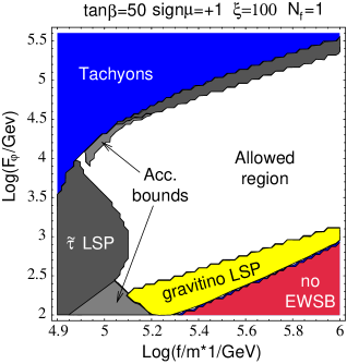
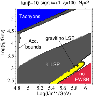
Figure 1: Excluded and allowed regions in the plane $(f/m,F_{\varphi})$

In fig. 1 we show the regions in the parameter space already excluded on phenomenological ground, the regions in which the neutralino is not the LSP (either gravitino or stau LSP) and the allowed regions for two different scenarios. In the left panel we fixed $\tan\beta=50$, $N_{f}=1$ and the messenger scale to $\xi=100$. The upper left regions (blue shaded region) is excluded due to the presence of tachyons in the spectrum (that is the minimal AMSB result) while the lower right region (red shaded region) is excluded due to an incorrect electroweak symmetry breaking (EWSB). The yellow shaded region is the region in which the gravitino is the LSP and it is determined by the condition

$$F_{\varphi}\leq m_{\chi}.$$ (5.30)

In the dark gray shaded region the lightest stau is the LSP. The light dark shaded region is excluded by the current accelerator constraints on the Higgs boson masses, $b\to s\gamma$, slepton masses, etc. In particular we considered the LEP2 lower bound [28] for the mass of the lightest SM-like Higgs boson $h_{0}$

$$m_{h_{0}}\geq 114.4\;\;{\rm GeV}$$ (5.31)

In the right panel of fig. 1 we show the excluded region for a scenario with $N_{f}=2$ messenger fields. In this case the tau LSP region is much wider and a new branch of an allowed region opens toward higher values of $f/m$. We will see in the following discussion that this branch is interesting from the point of view of the neutralino. In general, scenarios with $N_{f}\geq 1$ are less constrained by the current accelerator data.

There are only slight changes in the excluded and allowed regions for models with $\xi\lesssim 10$. In general the regions that contains tachyons and with no EWSB are much larger than the $\xi\simeq 100$ case. Models with $\xi\gtrsim 1000$ exhibit a much wider region in which the gravitino is the LSP and a smaller region with no EWSB.

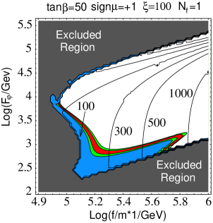
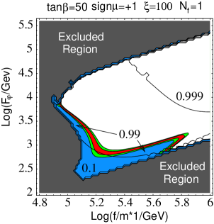
Figure 2: Contour plots in the plane $(f/m,F_{\varphi})$. Left panel: neutralino mass (expressed in GeV). Right panel: gaugino fraction.

We also computed the thermal relic density $\Omega_{\chi}h^{2}$ for the neutralino solving the Boltzmann equations in a standard cosmological scenario. We leave the analysis of some non standard cosmological scenario involving the presence of the moduli field associated to the supersymmetry breaking parameter $F_{\varphi}$ for future work. The lightest neutralino is given by the linear combination

$$\tilde{\chi}_{1}^{0}=N_{11}\tilde{B}+N_{12}\tilde{W}+N_{13}\tilde{H}_{u}+N_{14}\tilde{H}_{d}$$ (5.32)

where $\tilde{B}$ and $\tilde{W}$ are the bino and wino fields while $\tilde{H}_{u}$ and $\tilde{H}_{d}$ are the two higgsinos. We also define the gaugino fraction as

$$Z_{g}=\left|N_{11}\right|^{2}+\left|N_{12}\right|^{2}$$ (5.33)

We say that a neutralino is gaugino-like (in particular in our case bino-like) if $Z_{g}>0.9$ while is higgsino-like when $Z_{g}<0.1$. In all the intermediate cases we denote the neutralino as mixed-like.

We show the results for the $N_{f}=1$ scenario in fig. 2. In the left panel we show the neutralino isomass contours together with the cosmologically favorite regions: models in the red shaded region have a relic density in the $2\sigma$ WMAP [29] range $\Omega_{CDM}h^{2}=0.110\pm 0.014$ while models in the green region are in the $5\sigma$ range with $\Omega_{CDM}h^{2}=0.110\pm 0.035$. The blue region denotes models in which the neutralino is really a subdominant dark matter component with $\Omega_{\chi}h^{2}\lesssim 0.07$. The allowed neutralino masses range from $m_{\chi}\simeq 100$ GeV up to $m_{\chi}\simeq 1$ TeV while, as can be seen in the right panel of fig. 2. The neutralino is a very pure bino except in a very small region (which is in fact hardly visible in the figure) around the excluded zone in which $Z_{g}<0.1$, i.e. a very pure higgsino.

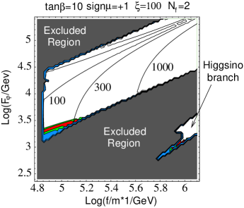
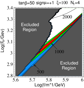
Figure 3: Neutralino mass (expressed in GeV) contour plots in the plane $(f/m,F_{\varphi})$ for $N_{f}>1$. Left panel: $N_{f}=2$ scenario. Right panel: higgsino region in the $N_{f}=4$ scenario.

The results for $N_{f}>1$ are shown in fig. 3. It is worth noting that in this case there is a new branch in the parameter space in the region of high $f/m$ (whose shape in general depends from $\xi$ and $\tan\beta$) in which the neutralino is a very pure higgsino. In the right panel of fig. 3 we show the higgsino region for $\tan\beta=50$ and $N_{f}=4$. The cosmologically allowed region is centered around $m_{\chi}\simeq 1$ TeV, that is a quite natural result for a heavy higgsino-like neutralino [30, 31]. This is due the fact that in this case the $W^{+}W^{-}$ channel (through a chargino exchange) and the $Z^{0}Z^{0}$ channel are no longer suppressed and thus this implies a higher annihilation cross section.

6 Conclusions

In this paper we showed that in the framework of the deflected anomaly mediated scenario, which solves the problem of the tachyons of the minimal anomaly mediation, the neutralino is still the LSP in a wide region of the parameter space. This is achieved considering the effects of the presence of a gauge mediated sector. While in the standard anomaly mediation the neutralino is wino like, this is no longer true for the scenario discussed here. In fact the neutralino turns out to be a very pure bino or a very pure higgsino depending on the number of messengers $N_{f}$ in the gauge mediated sector. We have also computed the thermal relic density (considering the standard cosmological scenario) and we found that there are regions compatible with the latest WMAP data both for $N_{f}=1$ and $N_{f}>1$.

Appendix A Extraction of the Soft Terms

In this appendix we derive the soft supersymmetry breaking terms starting from the lagrangian of eq. (4.27). Let us start by writing it in a more compact form:

$$L = \left[Z_{Q}\left(\rho^{2}+\delta\rho^{2},\sigma^{2}+\delta\sigma^{2}\right)Q^{\dagger}Q\right]_{\theta^{2}{\bar{\theta}}^{2}}+$$ (A.34)

$$+\left\{\left[y_{0}Q^{3}+g^{-2}\left(\rho+\delta\rho,\sigma+\delta\sigma\right){\cal{W}}{\cal{W}}\right]_{\theta^{2}}+h.c.\right\},$$

where we have defined the quantities:

$$\rho=\frac{\mu}{m}$$ (A.35)

$$\delta\rho=-\rho\theta^{2}\frac{f}{m}$$ (A.36)

$$\sigma=\frac{m}{\Lambda_{UV}}$$ (A.37)

$$\delta\sigma=\sigma\theta^{2}\left(\frac{f}{m}-F_{\varphi}\right)$$ (A.38)

$$\delta\rho^{2}=\rho^{2}\left(-\theta^{2}\frac{f}{m}-{\bar{\theta}}^{2}\frac{f}{m}+\theta^{2}{\bar{\theta}}^{2}\frac{f^{2}}{m^{2}}\right)$$ (A.39)

$$\delta\sigma^{2}=\sigma^{2}\left[\theta^{2}\left(\frac{f}{m}-F_{\varphi}\right)+{\bar{\theta}}^{2}\left(\frac{f}{m}-F_{\varphi}\right)+\theta^{2}{\bar{\theta}}^{2}\left(\frac{f}{m}-F_{\varphi}\right)^{2}\right].$$ (A.40)

After expanding eq. (A.34) around $(\rho,\sigma)$ and $(\rho^{2},\sigma^{2})$ , we can write the lagrangian as

$$L = \left\{\left[Z_{Q}^{i}(\rho^{2},\sigma^{2})+Z_{1}^{i}(\rho^{2},\sigma^{2})\left(\theta^{2}+{\bar{\theta}}^{2}\right)+Z_{2}^{i}(\rho^{2},\sigma^{2})\theta^{2}{\bar{\theta}}^{2}\right]Q^{\dagger}_{i}Q_{i}\right\}_{\theta^{2}{\bar{\theta}}^{2}}+$$ (A.41)

$$+\left\{\left[\frac{1}{6}y^{ijk}Q_{i}Q_{j}Q_{k}+\left(g^{-2}(\rho,\sigma)+\delta g^{-2}(\rho,\sigma)\theta^{2}\right){\cal{W}}{\cal{W}}\right]_{\theta^{2}}+\right.$$

$$\left.+h.c.\right\},$$

where we have posed:

$$Z_{1}^{i}(\rho^{2},\sigma^{2}) = -\frac{\partial Z_{Q}^{i}}{\partial\ln\rho^{2}}\frac{f}{m}+\frac{\partial Z_{Q}^{i}}{\partial\ln\sigma^{2}}\left(\frac{f}{m}-F_{\varphi}\right)$$

$$Z_{2}^{i}(\rho^{2},\sigma^{2}) = \frac{\partial Z_{Q}^{i}}{\partial\ln\rho^{2}}\frac{f^{2}}{m^{2}}+\frac{\partial Z_{Q}^{i}}{\partial\ln\sigma^{2}}\left(\frac{f}{m}-F_{\varphi}\right)^{2}+$$ (A.42)

$$+\frac{\partial^{2}Z_{Q}^{i}}{\partial^{2}\ln\rho^{2}}\frac{f^{2}}{m^{2}}+\frac{\partial^{2}Z_{Q}^{i}}{\partial^{2}\ln\sigma^{2}}\left(\frac{f}{m}-F_{\varphi}\right)^{2}+$$

$$-2\frac{f}{m}\left(\frac{f}{m}-F_{\varphi}\right)\frac{\partial^{2}Z_{Q}^{i}}{\partial\ln\rho^{2}\partial\ln\sigma^{2}}$$

and

$$\delta g^{-2}(\rho,\sigma)=-\frac{\partial g^{-2}}{\partial\ln\rho}\frac{f}{m}+\frac{\partial g^{-2}}{\partial\ln\sigma}\left(\frac{f}{m}-F_{\varphi}\right).$$ (A.43)

In eq. (A.41) we have introduced the flavor indices in the kinetic and trilinear superpotential terms for later convenience. In order to extract the soft supersymmetry breaking terms, we need to rescale the $Q_{i}$ and ${\cal{W}}$ chiral superfields in such a way that the new kinetic terms are canonically normalized. The suitable definitions are:

$$g^{-1}{\cal{W}}={\cal{W}}^{\prime}$$ (A.44)

$${Z_{Q}^{i}}^{\frac{1}{2}}\left(1+\frac{Z_{1}^{i}}{Z_{Q}^{i}}\theta^{2}\right)Q_{i}=Q_{i}^{\prime},$$ (A.45)

where $g^{-1}$ is evaluated at $(\rho,\sigma)$ and $Z_{Q}^{i},Z_{1}^{i}$ at $(\rho^{2},\sigma^{2})$. By expressing eq. (A.41) in terms of the new (primed) fields, we obtain that:

$$L = \left\{Q_{i}^{\prime\dagger}Q_{i}^{\prime}+\theta^{2}{\bar{\theta}}^{2}\left[\frac{Z_{2}^{i}}{Z_{Q}^{i}}-\frac{Z_{1}^{i2}}{Z_{Q}^{i2}}\right]Q_{i}^{\prime\dagger}Q_{i}^{\prime}\right\}_{\theta^{2}{\bar{\theta}}^{2}}+$$ (A.46)

$$+\left\{\left[{\cal{W}}^{\prime}{\cal{W}}^{\prime}+\theta^{2}\left(g^{2}\delta g^{-2}\right){\cal{W}}^{\prime}{\cal{W}}^{\prime}\right]_{\theta^{2}}\right\}+$$

$$+\left\{\left.\frac{1}{6}\frac{y^{ijk}}{\left({Z_{Q}^{i}}{Z_{Q}^{j}}{Z_{Q}^{k}}\right)^{\frac{1}{2}}}\left[1-\left(\frac{Z_{1}^{i}}{Z_{Q}^{i}}+\frac{Z_{1}^{j}}{Z_{Q}^{j}}+\frac{Z_{1}^{k}}{Z_{Q}^{k}}\right)\right]Q_{i}^{\prime}Q_{j}^{\prime}Q_{k}^{\prime}\right|_{\theta^{2}}+\right.$$

$$\left.+h.c.\right\}.$$

In our normalization (which is the same of [8]) the lowest component of the gauge field strength is ${\cal{W}}^{\prime}=-i\frac{\lambda^{\prime}}{2}$. By dropping the prime on all the fields and by redefining

$$\frac{y^{ijk}}{\left({Z_{Q}^{i}}{Z_{Q}^{j}}{Z_{Q}^{k}}\right)^{\frac{1}{2}}}\rightarrow y^{ijk},$$

we finally see that the lagrangian density with canonically normalized kinetic terms contains the following soft breaking interactions:

$$L \supset -\left[\frac{Z_{1}^{i2}}{Z_{Q}^{i2}}-\frac{Z_{2}^{i}}{Z_{Q}^{i}}\right]{\tilde{q}}_{i}^{*}{\tilde{q}}_{i}-\frac{1}{2}\left[\frac{1}{2}g^{2}\delta g^{-2}\right]\lambda\lambda+$$ (A.47)

$$-\frac{1}{6}\left[\left(\frac{Z_{1}^{i}}{Z_{Q}^{i}}+\frac{Z_{1}^{j}}{Z_{Q}^{j}}+\frac{Z_{1}^{k}}{Z_{Q}^{k}}\right)y^{ijk}\right]{\tilde{q}}_{i}{\tilde{q}}_{j}{\tilde{q}}_{k}+h.c.$$

By comparing with the lagrangian (4.20), we can read off the soft supersymmetry breaking parameters:

$$M_{\lambda} = \frac{1}{2}g^{2}\delta g^{-2}$$

$$m_{ij}^{2} = \left(\frac{Z_{1}^{i2}}{Z_{Q}^{i2}}-\frac{Z_{2}^{i}}{Z_{Q}^{i}}\right)\delta_{ij}$$ (A.48)

$$a_{ijk} = \left(\frac{Z_{1}^{i}}{Z_{Q}^{i}}+\frac{Z_{1}^{j}}{Z_{Q}^{j}}+\frac{Z_{1}^{k}}{Z_{Q}^{k}}\right)y^{ijk}$$

$$b_{ij} = 0$$

Note that we are not providing any solution for the $\mu$ problem. Now we derive explicit expressions for the soft breaking parameters in terms of low energy observable quantities.

Appendix B Explicit Expressions for the Soft Terms

We need to compute the wave function renormalizations and the gauge couplings at an arbitrary renormalization scale $\mu$ of the order of the typical mass of the MSSM particles. The one loop order RG equation for the running gauge coupling is given by

$$\frac{d}{d\ln\mu}g=-\frac{b}{16\pi^{2}}g^{3},$$ (B.49)

where $b$ is the appropriate one loop $\beta$-function coefficient at the scale $\mu$. We need to integrate eq. (B.49) between the low energy scale $\mu$ and the UV cutoff scale $\Lambda_{UV}$. We have to consider that if we denote with $b$ the $\beta$-function coefficient at the low energy scale, then above the messenger mass scale $m$ the $\beta$-function coefficient becomes $b^{\prime}=b-N_{f}$, where $N_{f}$ is the number of flavors of messengers running into the loops for $\mu>m$. In passing through the threshold $m$ when integrating eq. (B.49), we match the values of the running gauge couplings above and below $m$. The computation yields

$$g^{-2}\left(\rho,\sigma\right)=g^{-2}(\Lambda_{UV})+\frac{b-N_{f}}{8\pi^{2}}\ln\sigma+\frac{b}{8\pi^{2}}\ln\rho,$$ (B.50)

where the variables $\rho$ and $\sigma$ are defined in eqs. (A.35) and (A.37). With a similar calculation and using the last result, we can integrate the RG equation of the wave function renormalization $Z_{Q}^{i}$. This, in the limit of small Yukawa couplings with respect to $g^{2}$, is given by

$$\frac{d}{d\ln\mu}\ln Z_{Q}^{i}=\sum_{G_{Q_{i}}}\frac{c}{4\pi^{2}}g^{2}.$$ (B.51)

In the last formula the sum is extended to all the gauge groups under which $Q^{i}$ is charged and $c$ is the relative quadratic Casimir. The result of the integration can be written as

$$\ln Z_{Q}^{i}\left(\rho^{2},\sigma^{2}\right)=\ln Z_{Q}^{i}\left(\Lambda_{UV}\right)+$$

$$+\sum_{G_{Q_{i}}}\left\{\frac{2c}{b-N_{f}}\ln\left[\frac{g^{-2}(\Lambda_{UV})+\frac{b-N_{f}}{8\pi^{2}}\ln\sigma}{g^{-2}(\Lambda_{UV})}\right]+\right.$$

$$\left.+\frac{2c}{b}\ln\left[\frac{g^{-2}(\Lambda_{UV})+\frac{b-N_{f}}{8\pi^{2}}\ln\sigma+\frac{b}{8\pi^{2}}\ln\rho}{g^{-2}(\Lambda_{UV})+\frac{b-N_{f}}{8\pi^{2}}\ln\sigma}\right]\right\}.$$ (B.52)

To compute the soft breaking parameters listed in eq. (A), we need to use eqs. (B.50), (B.52) into eqs. (A.42), (A.43) and plug the result into eq. (A). The soft breaking parameters that arise from such computation are

$$m^{2}_{ij}(\mu) = \delta_{ij}\sum_{G_{i}}\frac{2cg^{4}(\mu)}{(4\pi)^{4}}\left\{\left(\frac{f}{m}\right)^{2}N_{f}\left[\zeta^{2}+\frac{N_{f}}{b}(1-\zeta^{2})\right]+\right.$$

$$+F_{\varphi}^{2}\left[b+N_{f}\left(\zeta^{2}-2+\frac{N_{f}}{b}(1-\zeta^{2})\right)\right]+$$

$$+\left.\frac{2fF_{\varphi}}{m}N_{f}(1-\zeta^{2})\left(1-\frac{N_{f}}{b}\right)\right\}$$

$$M_{\lambda}(\mu) = -\frac{g^{2}(\mu)}{(4\pi)^{2}}\left[N_{f}\frac{f}{m}+(b-N_{f})F_{\varphi}\right]$$ (B.53)

$$a_{ijk}(\mu) = \sum_{G_{i},G_{j},G_{k}}\frac{2cg^{2}(\mu)}{(4\pi)^{2}}\left\{\frac{f}{m}\frac{N_{f}}{b}(\zeta-1)\right.+$$

$$-\left.F_{\varphi}\left[1+\frac{N_{f}}{b}(\zeta-1)\right]\right\}y_{ijk}$$

where we have defined

$$\zeta(\mu)=\left[1+\frac{bg^{2}(\mu)}{8\pi^{2}}\ln\left(\frac{m}{\mu}\right)\right]^{-1}=\left[1-\frac{bg^{2}(\mu)}{8\pi^{2}}\alpha(\mu)\ln\rho\right]^{-1}.$$ (B.54)

It is important to check that from eq. (B), in the limit in which the GMSB-like contribution to the soft terms decouples, we can recover the standard AMSB results for the soft terms. This is easy to verify, since in the decoupling case $f/m=F_{\varphi}$ we get:

$$m^{2}_{ij}(\mu) = \delta_{ij}\sum_{G_{i}}\frac{2cg^{4}(\mu)}{(4\pi)^{4}}bF_{\varphi}^{2}$$

$$M_{\lambda}(\mu) = -\frac{g^{2}(\mu)}{(4\pi)^{2}}bF_{\varphi}$$ (B.55)

$$a_{ijk}(\mu) = -\sum_{G_{i},G_{j},G_{k}}\frac{2cg^{2}(\mu)}{(4\pi)^{2}}F_{\varphi}y_{ijk}$$

which are the standard AMSB results of [6]. In the phenomenological study we are interested in, we give the boundary conditions for the soft terms at the renormalization scale $\mu=m$, which corresponds to the typical messenger mass. At such scale the results of eq. (B) simplify, since $\zeta(m)=1$. We can then write:

$$\left.m_{\lambda}\right|_{\mu=m} = -\frac{g^{2}(m)}{(4\pi)^{2}}\left[N_{f}\frac{f}{m}+(b-N_{f})F_{\varphi}\right]$$

$$\left.m^{2}_{ij}\right|_{\mu=m} = \delta_{ij}\sum_{G_{i}}\frac{2cg^{4}(m)}{(4\pi)^{4}}\left[\left(\frac{f}{m}\right)^{2}N_{f}+F_{\varphi}^{2}\left(b-N_{f}\right)\right]$$ (B.56)

$$\left.a_{ijk}\right|_{\mu=m} = -\sum_{G_{i},G_{j},G_{k}}\frac{2cg^{2}(m)}{(4\pi)^{2}}F_{\varphi}y_{ijk}$$

We observe that in (B) the soft terms at the messenger scale are exactly the sum of the AMSB-like and GMSB-like contributions. In table 1 we report the values of the one loop $\beta$-function coefficients and the quadratic Casimirs for the standard model gauge groups and particles.

$$\begin{array}[]{|c|c|c|c|}\hline\cr\mbox{Field}&c_{1}&c_{2}&c_{3}\\ \hline\cr Q&1/60&3/4&4/3\\ t&4/15&&4/3\\ b&1/15&&4/3\\ L&3/20&3/4&\\ \tau&3/5&&\\ H_{u}&3/20&3/4&\\ H_{d}&3/20&3/4&\\ \hline\cr\end{array}\hskip 14.22636pt\begin{array}[]{|c|c|}\hline\cr\mbox{Group}&b\\ \hline\cr U(1)_{Y}&-33/5\\ SU(2)_{L}&-1\\ SU(3)_{C}&3\\ \hline\cr\end{array}$$

Table 1: Quadratic Casimirs for the MSSM particles and one loop $\beta$-function coefficients for the gauge groups (the indices $1,2,3$ indicate the $U(1)_{Y}$, $SU(2)_{L}$, $SU(3)_{C}$ gauge groups respectively).

To obtain our final predictions for the soft supersymmetry breaking terms at the renormalization scale $m$ and in the limit of small Yukawa couplings, we only have to put values contained in table 1 into eq. (B).

The results are listed in the following equations.

$$\left.M_{1}\right|_{\mu=m} = -\frac{g_{1}^{2}(m)}{(4\pi)^{2}}\left[N_{f}\frac{f}{m}+(-\frac{33}{5}-N_{f})F_{\varphi}\right]$$

$$\left.M_{2}\right|_{\mu=m} = -\frac{g_{2}^{2}(m)}{(4\pi)^{2}}\left[N_{f}\frac{f}{m}+(-1-N_{f})F_{\varphi}\right]$$ (B.57)

$$\left.M_{3}\right|_{\mu=m} = -\frac{g_{3}^{2}(m)}{(4\pi)^{2}}\left[N_{f}\frac{f}{m}+(3-N_{f})F_{\varphi}\right]$$

$$\left.A_{t}\right|_{\mu=m} = -\frac{1}{(4\pi)^{2}}\left(\frac{16}{3}g_{3}^{2}+3g_{2}^{2}+\frac{13}{15}g_{1}^{2}\right)y_{t}$$

$$\left.A_{b}\right|_{\mu=m} = -\frac{1}{(4\pi)^{2}}\left(\frac{16}{3}g_{3}^{2}+3g_{2}^{2}+\frac{7}{15}g_{1}^{2}\right)y_{b}$$ (B.58)

$$\left.A_{\tau}\right|_{\mu=m} = -\frac{1}{(4\pi)^{2}}\left(3g_{2}^{2}+\frac{9}{5}g_{1}^{2}\right)y_{\tau}$$

$$\left.{\tilde{m}}_{Q}^{2}\right|_{\mu=m} = diag(1,1,1)\times\frac{2}{(4\pi)^{4}}\left\{\left[\left(\frac{f}{m}\right)^{2}N_{f}+(3-N_{f})F_{\varphi}^{2}\right]\frac{4}{3}g_{3}^{4}(m)\right.+$$

$$+\left[\left(\frac{f}{m}\right)^{2}N_{f}+(-1-N_{f})F_{\varphi}^{2}\right]\frac{3}{4}g_{2}^{4}(m)+$$

$$\left.+\left[\left(\frac{f}{m}\right)^{2}N_{f}+\left(-\frac{33}{5}-N_{f}\right)F_{\varphi}^{2}\right]\frac{1}{60}g_{1}^{4}(m)\right\}$$

$$\left.{\tilde{m}}_{t}^{2}\right|_{\mu=m} = diag(1,1,1)\times\frac{2}{(4\pi)^{4}}\left\{\left[\left(\frac{f}{m}\right)^{2}N_{f}+(3-N_{f})F_{\varphi}^{2}\right]\frac{4}{3}g_{3}^{4}(m)\right.+$$

$$\left.+\left[\left(\frac{f}{m}\right)^{2}N_{f}+\left(-\frac{33}{5}-N_{f}\right)F_{\varphi}^{2}\right]\frac{4}{15}g_{1}^{4}(m)\right\}$$

$$\left.{\tilde{m}}_{b}^{2}\right|_{\mu=m} = diag(1,1,1)\times\frac{2}{(4\pi)^{4}}\left\{\left[\left(\frac{f}{m}\right)^{2}N_{f}+(3-N_{f})F_{\varphi}^{2}\right]\frac{4}{3}g_{3}^{4}(m)\right.+$$

$$\left.+\left[\left(\frac{f}{m}\right)^{2}N_{f}+\left(-\frac{33}{5}-N_{f}\right)F_{\varphi}^{2}\right]\frac{1}{15}g_{1}^{4}(m)\right\}$$

$$\left.{\tilde{m}}_{L}^{2}\right|_{\mu=m} = diag(1,1,1)\times\frac{2}{(4\pi)^{4}}\left\{\left[\left(\frac{f}{m}\right)^{2}N_{f}+(-1-N_{f})F_{\varphi}^{2}\right]\frac{3}{4}g_{2}^{4}(m)\right.+$$

$$\left.+\left[\left(\frac{f}{m}\right)^{2}N_{f}+\left(-\frac{33}{5}-N_{f}\right)F_{\varphi}^{2}\right]\frac{3}{20}g_{1}^{4}(m)\right\}$$

$$\left.{\tilde{m}}_{\tau}^{2}\right|_{\mu=m} = diag(1,1,1)\times\frac{2}{(4\pi)^{4}}\left\{\left[\left(\frac{f}{m}\right)^{2}N_{f}+\left(-\frac{33}{5}-N_{f}\right)F_{\varphi}^{2}\right]\frac{3}{5}g_{1}^{4}(m)\right\}$$

$$\left.{m}_{H_{u}}^{2}\right|_{\mu=m} = \left.{m}_{H_{d}}^{2}\right|_{\mu=m}=\frac{2}{(4\pi)^{4}}\left\{\left[\left(\frac{f}{m}\right)^{2}N_{f}+(-1-N_{f})F_{\varphi}^{2}\right]\frac{3}{4}g_{2}^{4}(m)\right.+$$

$$\left.+\left[\left(\frac{f}{m}\right)^{2}N_{f}+\left(-\frac{33}{5}-N_{f}\right)F_{\varphi}^{2}\right]\frac{3}{20}g_{1}^{4}(m)\right\}$$

References

- [1] G. Jungman, M. Kamionkowski and K. Griest, Phys. Rept. 267, 195 (1996).
- [2] D. J. H. Chung, L. L. Everett, G. L. Kane, S. F. King, J. Lykken and L. T. Wang, Phys. Rept. 407, 1 (2005).
- [3] Y. Shadmi, arXiv:hep-th/0601076.
-
[4]
Hall L J, Lykken J, and Weinberg S 1983 Phys. Rev. D 27 2359
N. Ohta, Prog. Theor. Phys. 70 (1983) 542. - [5] G. F. Giudice and R. Rattazzi, Phys. Rept. 322 (1999) 419
- [6] L. Randall and R. Sundrum, Nucl. Phys. B 557 (1999) 79
- [7] S. P. Martin, arXiv:hep-ph/9709356.
- [8] J. Bagger, J. Wess, Supersymmetry and Supergravity, Princeton Series in Physics, Second Edition
- [9] L. Randall and R. Sundrum, Phys. Rev. Lett. 83 (1999) 3370
- [10] L. Randall and R. Sundrum, Phys. Rev. Lett. 83 (1999) 4690
- [11] M. A. Luty and R. Sundrum, Phys. Rev. D 64 (2001) 065012
- [12] N. Okada, Phys. Rev. D 65 (2002) 115009
-
[13]
A. Pomarol and R. Rattazzi,
JHEP 9905 (1999) 013
R. Rattazzi, A. Strumia and J. D. Wells, Nucl. Phys. B 576 (2000) 3 - [14] G. F. Giudice, M. A. Luty, H. Murayama and R. Rattazzi, JHEP 9812 (1998) 027
- [15] M. A. Luty and R. Sundrum, Phys. Rev. D 62 (2000) 035008
- [16] M. A. Luty and R. Sundrum, Phys. Rev. D 65 (2002) 066004
- [17] M. Luty and R. Sundrum, Phys. Rev. D 67 (2003) 045007
- [18] I. Jack and D. R. T. Jones, Phys. Lett. B 482 (2000) 167
- [19] N. Arkani-Hamed, D. E. Kaplan, H. Murayama and Y. Nomura, JHEP 0102 (2001) 041
- [20] E. Katz, Y. Shadmi and Y. Shirman, JHEP 9908 (1999) 015
- [21] Z. Chacko, M. A. Luty, I. Maksymyk and E. Ponton, JHEP 0004 (2000) 001
- [22] B. C. Allanach and A. Dedes, JHEP 0006 (2000) 017
- [23] Z. Chacko and M. A. Luty, JHEP 0205 (2002) 047
- [24] Z. Chacko and E. Ponton, Phys. Rev. D 66 (2002) 095004
- [25] S. P. Martin and M. T. Vaughn, Phys. Rev. D 50 (1994) 2282
- [26] F. E. Paige, S. D. Protopopescu, H. Baer and X. Tata, arXiv:hep-ph/0312045.
- [27] P. Gondolo, J. Edsjo, P. Ullio, L. Bergstrom, M. Schelke and E. A. Baltz, JCAP 0407 (2004) 008
- [28] W. M. Yao et al. [Particle Data Group], J. Phys. G 33 (2006) 1.
- [29] D. N. Spergel et al., arXiv:astro-ph/0603449.
- [30] J. Edsjo and P. Gondolo, Phys. Rev. D 56 (1997) 1879
- [31] U. Chattopadhyay, D. Choudhury, M. Drees, P. Konar and D. P. Roy, Phys. Lett. B 632 (2006) 114