Potential Models and Lattice Gauge Current-Current Correlators

Abstract

We compare current-current correlators in lattice gauge calculations with correlators in different potential models, for a pseudoscalar charmonium in the quark-gluon plasma. An important ingredient in the evaluation of the current-current correlator in the potential model is the basic principle that out of the set of continuum states, only resonance states and Gamow states with lifetimes of sufficient magnitudes can propagate as composite objects and can contribute to the current-current correlator. When the contributions from the bound states and continuum states are properly treated, the potential model current-current correlators obtained with the potential proposed in Ref. [11] are consistent with the lattice gauge correlators. The proposed potential model thus gains support to be a useful tool to complement lattice gauge calculations for the study of $Q\bar{Q}$ states at high temperatures.

I Introduction

Potential models have often been used to describe bound states of quark-antiquark pairs. The basic idea is that a short range attractive color-Coulomb interaction with a long-range confining interaction provides an adequate account of the interaction between a quark and antiquark. While the non-relativistic potential model was originally introduced for heavy quarkonium systems, relativistic and non-relativistic quark models using constituent quark masses have been used to describe mesons with one or two light quarks as quark-antiquark bound states God85 ; Bar92 ; Won02 ; Cra04 ; Cra06 .

Potential models have also been used to study heavy quarkonium bound states at high temperatures Mat86 ; Dig01a ; Won01a ; Kac02 ; Shu03 ; Won05 ; Won05a ; Won06 ; Won06a ; Son05 ; Alb05 ; Bla05 ; Man05 ; Dig05 . At temperatures above the phase transition temperature, the potential between a quark and an antiquark is subject to screening Mat86 . Heavy quarkonium states become unbound in the potential as temperature rises. Potential models provide beneficial complements to lattice gauge calculations as potential models allow simple and intuitive evaluations of many quantities, some of which may be beyond the scope of present-day lattice gauge calculations. The central question in the potential model has been focused on the characteristics and the temperature dependencies of the screening potential as determined by lattice gauge calculations Mat86 ; Dig01a ; Won01a ; Kac02 ; Shu03 ; Won05 ; Won05a ; Won06 ; Won06a ; Son05 ; Alb05 ; Bla05 ; Man05 ; Dig05 .

There is recently a serious theoretical question whether it is appropriate to apply a potential model to study heavy quarkonia at high temperatures Moc06 ; Moc06a . On the one hand, lattice gauge spectral function analyses have been carried out to investigate the stability of heavy quarkonia at high temperatures Asa03 ; Mat01 ; Dat03 ; Pet05 ; Jak06 . On the other hand, independent lattice gauge calculations Kac03 ; Kac05 have been performed to evaluate various thermodynamical quantities, such as the free energy $F_{1}({\bf r},T)$ and the internal energy $U_{1}({\bf r},T)$, for a color-singlet static $Q$-$\bar{Q}$ pair at various separations ${\bf r}$ and temperatures $T$. It remains an important open theoretical question how a quark-antiquark potential can be extracted from these thermodynamical quantities. Various potential models have been proposed, utilizing $F_{1}$ Dig01a ; Won01a ; Bla05 , $U_{1}$ Kac02 ; Shu03 ; Alb05 ; Man05 , or a linear combination of $F_{1}$ and $U_{1}$ with coefficients that depend on the equation of state Won05 ; Won05a ; Won06 ; Won06a . Although the latter linear-combination model has been justified by theoretical arguments and leads to dissociation temperatures that are consistent with lattice gauge spectral function dissociation temperatures Won05 ; Won05a ; Won06 ; Won06a , it remains necessary to confront the model with other lattice gauge data to assess the degree of its usefulness.

The spectral function is related to the meson current-current correlator by a generalized Laplace transform. In principle, they carry equivalent information on the composite system. One would expect intuitively that the consistency of the lattice gauge spectral function dissociation temperatures with the potential model dissociation temperatures using the potential of Won05 would lead to consistency of the lattice gauge correlators with the corresponding potential model correlators. Recent works in Refs. Moc06 ; Moc06a however make the contrary claim that the meson correlators obtained with many different types of potential models are not consistent with lattice gauge correlators, and consequently potential models cannot describe heavy quarkonia above $T_{c}$.

The failure of the potential model correlators to reproduce lattice gauge correlators in Refs. Moc06 ; Moc06a for all cases suggests that the lack of agreement may not be due to the potential models themselves but to the method of evaluating the meson correlators in the potential model. In the work of Ref. Moc06 ; Moc06a , continuum states arising from a free fermion $Q$ and $\bar{Q}$ pair in a fermion gas contribute to the correlator. However, to be able to propagate as a composite meson so as to contribute to the correlator, the quark and the antiquark must be temporally and spatially correlated to be a composite object with a sufficiently long lifetime. Continuum states in the free quark and antiquark gas may not have sufficient temporal and spatial correlations to be composite objects for such a propagation.

While we raise questions on the method of evaluating the potential model correlators in Moc06 ; Moc06a , we wish to present what we view as a proper treatment of the current-current correlator in the potential model. We wish to point out the basic principle that out of the continuum states, only resonance states and Gamow states footnote with lifetimes of sufficient magnitude can propagate as composite objects and contribute to the meson current-current correlator. With the simple example of the pseudoscalar correlator, we shall show in this paper that when both the bound state and the continuum state contributions are properly treated, the potential model of Won05 using a linear combination of $F_{1}({\bf r},T)$ and $U_{1}({\bf r},T)$ yields correlators consistent with lattice gauge correlators, while the $F_{1}$ potential and the $U_{1}$ potential lead to deviations. Our results indicate consistency of the potential model of Won05 with both the lattice gauge spectral function analyses and the lattice gauge correlator analyses. The potential model of Won05 thus gains support to be a useful tool to complement lattice gauge calculations for the study of $Q\bar{Q}$ states at high temperatures.

In Section II, we review the basic assumptions in the treatment of the continuum states in Refs. Moc06 ; Moc06a . We review in Section III the relationship between the current-current correlator and the quarkonium wave functions. In Section IV, we show how the resonance states and Gamow states are characterized in the potential model. In Section V, the potential model correlator is expressed as a sum over contributions from meson bound and continuum states with lifetimes greater than a certain limit. In Section VI, we discuss the relation between the $Q$-$\bar{Q}$ potential and lattice gauge thermodynamic quantities. In Section VII, we evaluate the potential model correlators and find that the correlators obtained with the potential of Won05 have features similar to those of lattice gauge correlators. We have thus demonstrated the consistency of the potential model correlators with lattice gauge correlators. In Section VIII, we discuss the implications of the potential model analysis on the assume default spectrum in the lattice gauge spectral function analysis. In Section IX we present our conclusions.

II Meson Correlators and Continuum States

The meson (current-current) correlators $G(\tau,{\bf X})$ is a function of the Euclidean time $\tau$ and the spatial coordinate ${\bf X}$ defined by

$$G(\tau,\mathbf{X})=\langle J_{M}(\tau,\mathbf{X})J_{M}^{\dagger}(0,\mathbf{0})\rangle,$$ (1)

where $J_{M}(\tau,{\bf X})=\bar{q}(\tau,{\bf X})\Gamma_{M}q(\tau,{\bf X})$ and $\Gamma_{M}=1,\gamma^{5},\gamma^{\mu},\gamma^{5}\gamma^{\mu}$ are the operators appropriate for scalar, pseudoscalar, vector, and axial-vector mesons respectively. It is the probability amplitude for creating a meson $M$ at space-time point $(0,{\bf 0})$, propagating the meson to $(\tau,{\bf X})$, and destroying the meson at $(\tau,{\bf X})$. Specializing to the case of the meson momentum ${\bf P}$ equal to ${\bf 0}$, the meson correlator depends then on the meson mass spectrum $\sigma(\omega,T)$.

In their test of the potential model, the authors of Moc06 ; Moc06a assume that the meson mass spectrum in the potential model is given by

$$\sigma(\omega,T)=\sum_{i}2M_{i}F_{i}\delta(\omega^{2}-M_{i}^{2})+\frac{4}{8\pi^{2}}\theta(\omega-s_{0})(a_{H}+b_{H}\frac{s_{0}^{2}}{\omega^{2}})\sqrt{1-\frac{s_{0}^{2}}{\omega^{2}}},$$ (2)

where $M_{i}(T)$ is a bound state meson mass calculated in the potential model, $F_{i}(T)$ is the corresponding magnitude of the wave function at the origin. The second term with the step function represents continuum meson states obtained by assuming that the $Q$ and $\bar{Q}$ are free fermions in a fermion gas Kar01 . The quantity $s_{0}(T)$ is the continuum threshold, $a_{H}$ and $b_{H}$ are constants that depend on the meson type. The potential model meson correlator $G(\tau)$ is then obtained by folding the meson mass spectrum $\sigma(\omega,T)$ with the propagating kernel $K(\tau,\omega,T)$,

$$G(\tau)=\int d\omega\sigma(\omega,T)K(\tau,\omega,T),$$ (3)

where $K(\tau,\omega,T)$ is given by

$$K(\tau,\omega,T)=\frac{\cosh[\omega(\tau-1/2T)]}{\sinh[\omega/2T]}.$$ (4)

The lattice gauge correlator $G(\tau)$ is represented relative to the “reconstructed” correlator $G_{\rm recon}(\tau)$ calculated with the meson mass spectrum at $T=0$ Dat03 ; footnote2 . The lattice gauge pseudoscalar correlators obtained in Dat03 are shown in Fig. 1a. The potential model correlators $G(\tau)/G_{\rm recon}(\tau)$, obtained in Moc06 ; Moc06a with a screening potential (Fig. 1b) or with the potential of Ref. Won05 ; Won06 (Fig. 1c), are found to be qualitatively very different from the lattice gauge correlators of Fig. 1a. Significant differences occur for both charmonia and bottomia, at all temperatures above $T_{c}$, and for many fundamentally different potentials. The authors of Ref. Moc06 ; Moc06a then draw the conclusion that the potential model is not a good description for heavy quarkonia above $T_{c}$.

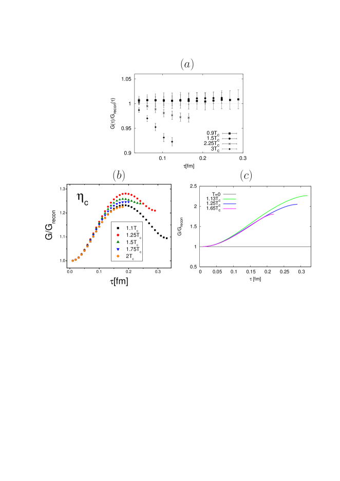
Figure 1: Fig. 1a shows the pseudoscalar charmonium correlators $G(\tau)/G_{\rm recon}(\tau)$ obtained in lattice gauge calculations Dat03 ; footnote2 . Fig. 1b shows the potential model correlators for the pseudoscalar charmonium obtained in Ref. Moc06 with the screened Cornell potential. Fig. 1c gives the potential model correlators for the pseudoscalar charmonium obtained in Ref. Moc06a with the potential of Refs. Won05 ; Won06 .

In the evaluations of the potential model correlators in Moc06 ; Moc06a , contributions from continuum states represented by the second term in Eq. (2) have been included. While the spectrum in the continuum states is continuous as in Eq. (2), not all continuum states represented by the step function $Q\bar{Q}$ free-fermion gas states in the second term in Eq. (2) possess the proper characteristics to propagate as a composite meson so as to contribute to the meson correlator $G(\tau)$. To be able to propagate as a composite meson from time 0 to $\tau$ so as to contribute to the correlator $G(\tau)$, the quark and antiquark must be temporally and spatially correlated. The composite object must have a composite lifetime sufficiently long compared to the propagation time $\tau$. Continuum states in the free quark and antiquark gas may not have sufficient temporal and spatial correlations between $Q$ and $\bar{Q}$ to qualify as being composite objects for such a propagation.

A similar question poses itself in low-energy nuclear physics in the evaluation of the density of continuum states of a composite object formed by a particle (neutron, say) and a nucleus (represented by a potential well). States for the free particle in a (neutron) fermion gas do not have relative temporal and spatial correlations between the particle and the nucleus to qualify as being a composite object formed by the particle and the nucleus in the continuum. It is for this well-known reason that to get the level density of continuum states of a composite object formed by a particle and a nucleus, it is necessary to subtract the level density of free gas states from the total density of continuum states Tub79 ; Shl92 ; Shl95 ; Shl97 ; Cha05 ; Alh03 . In the analogous problem of level density of continuum states of a composite $Q\bar{Q}$ meson, one can carry out the free fermion gas states subtraction or alternatively use only resonance states and Gamow states as contributors to the continuum level density Tub79 ; Shl92 ; Shl95 ; Shl97 ; Cha05 ; Alh03 . Therefore, for our case of meson correlators for a composite $Q\bar{Q}$ meson, the basic principle is that the proper continuum meson states that can contribute to the meson correlator $G(\tau)$ should be limited to meson resonance states and Gamow states which have composite object lifetime long compared to $\tau$. By focusing our attention on the pseudoscalar charmonium as an example, we would like to demonstrate that the potential model with the correct set of bound and continuum Gamow states can describe lattice gauge correlators.

III The Meson Correlator and Meson Internal Wave functions

We start with the current-current correlator $G(\tau,\mathbf{X})=\langle J_{M}(\tau,\mathbf{X})J_{M}^{\dagger}(0,\mathbf{0})\rangle$ of Eq. (1) and restrict ourselves to the consideration of the pseudoscalar charmonium. The current operator is just $J_{M}(\tau,\mathbf{X})=\bar{q}(\tau,\mathbf{X})\gamma_{5}q(\tau,\mathbf{X})$. The field operator has both annihilation and creation parts, $q(\tau,\mathbf{X})=q^{(+)}(\tau,\mathbf{X})+q^{(-)}(\tau,\mathbf{X})$.  Hence, the current operator can be decomposed into

$$J_{M}(\tau,\mathbf{X})=\bar{q}^{(-)}(\tau,\mathbf{X})\gamma_{5}q^{(+)}(\tau,\mathbf{X})+\bar{q}^{(+)}(\tau,\mathbf{X})\gamma_{5}q^{(+)}(\tau,\mathbf{X})+\bar{q}^{(-)}(\tau,\mathbf{X})\gamma_{5}q^{(-)}(\tau,\mathbf{X})+\bar{q}^{(+)}(\tau,\mathbf{X})\gamma_{5}q^{(-)}(\tau,\mathbf{X}).$$ (5)

We consider the propagation of the pseudoscalar meson $M$ from the initial (Euclidean) space-time coordinate $(0,\mathbf{0})$ to the final space-time coordinate $(\tau,\mathbf{X})$. It is often convenient to study

$$G(\tau)=\int d\mathbf{X}G(\tau,\mathbf{X})=\int d\mathbf{X}\langle J_{M}(\tau,\mathbf{X})J_{M}^{\dagger}(0,\mathbf{0})\rangle.$$ (6)

The temporal behavior of the correlator $G(\tau)$ provides information on the meson spectrum.

For the extraction of information on the correlator we focus only on the particle-antiparticle creation operator portion $\bar{q}^{(+)}(\tau,\mathbf{X})\gamma_{5}q^{(-)}(\tau,\mathbf{X})~{}$ of Eq. (5). The $\gamma_{5}$ matrix singles out the dominant lower component of the operator $q^{(-)}(\tau,\mathbf{X})~{}$ for the antiquarks. We rename that dominant component by using the notation

$$J_{M}(\tau,\mathbf{X})=\psi_{1}(x_{1})\psi_{2}(x_{2}){\biggr{|}}_{x_{1}=x_{2}=(\tau,\mathbf{X})},$$ (7)

where particle 1 represents $Q$ and particle 2 represents $\bar{Q}$, $\psi_{1}(x_{1})$ and $\psi_{2}(x_{2})$ are the dominant $Q$ and $\bar{Q}$ fields. The meson current-current correlator of Eq. (1) becomes

$$G(\tau,\mathbf{X})=\langle~{}\psi_{1}(x_{1})\psi_{2}(x_{2})\psi_{1}^{\dagger}(x_{1}^{\prime})\psi_{2}^{\dagger}(x_{2}^{\prime})~{}\rangle{\biggr{|}}_{x_{1}=x_{2}=(\tau;\mathbf{X});x_{1}^{\prime}=x_{2}^{\prime}=(0,\mathbf{0})}.$$ (8)

The above current $J_{M}(\tau,\mathbf{X})$ is a local current where $(\tau,\mathbf{X})=X$ is the CM coordinate $X$ of the $Q$-$\bar{Q}$ pair with $X=(x_{1}+x_{2})/2$, and the relative coordinate, $x=(x_{1}-x_{2})$, is restricted to be zero. A general current containing a more general relative coordinate $x=(x_{1}-x_{2})$ is

$$J_{M}(X,x)=\psi_{1}(X+x/2)\psi_{2}(X-x/2),$$ (9)

with the more general Green’s function

$$G(x_{1},x_{2};x_{1}^{\prime},x_{2}^{\prime})=\langle\psi_{1}(x_{1})\psi_{2}(x_{2})\psi_{1}^{\dagger}(x_{1}^{\prime})\psi_{2}^{\dagger}(x_{2}^{\prime})\rangle.$$ (10)

We would like to make a transformation of the coordinate system from the separate particle coordinates $(x_{1},x_{2})$ to $(X,x)$ and introduce the field operator $\hat{\Psi}_{M}(X)$ to represent the field of a composite meson which has the internal relative motion between the quark and the antiquark described by an internal wave function $\psi_{M}$.

Following Won00 , we define the field operator ${\hat{\Psi}}_{M}(X)$ for CM motion by

$${\hat{\Psi}}_{M}(X)|X\rangle=\Psi_{M}(X)|X\rangle,$$ (11)

with the wave function $\Psi_{M}(X)$ satisfying Eq. (2.23) of Won00

$$\left\{P^{2}-M^{2}\right\}\Psi_{M}(X)=0,$$ (12)

where $P=p_{1}+p_{2}$ is the total momentum of $Q$ and $\bar{Q}$, $p_{1}$ is the momentum of of $Q$, and $p_{2}$ is the momentum of $\bar{Q}$. For each composite state of mass $M$, there is a wave function ${{\psi}}_{M}(x_{\perp})$ for relative motion satisfying Eq. (2.24) of Won00

$$\left\{p^{2}-\Phi(x_{\perp},M)+b^{2}(M^{2},m_{1}^{2},m_{2}^{2})\right\}\psi_{M}(x_{\perp})=0,$$ (13)

where $p=(p_{1}-p_{2})/2$ is the relative momentum of $Q$ and $\bar{Q}$, $\Phi(x_{\perp},M)$ is the two-body interaction potential that acts between $Q$ and $\bar{Q}$, and

$$x_{\perp} = x-\frac{PP\cdot x}{P^{2}},$$ (14)

$$P\cdot x_{\perp} = 0.$$ (15)

The composite particle mass $M$ is the constant of the separation of variables and is related to the eigenvalue $b^{2}$ of the Schrödinger-type equation for relative motion, Eq. (13), by

$$b^{2}(M^{2},m_{1}^{2},m_{2}^{2})=\frac{1}{4M^{2}}\{M^{4}-2M^{2}(m_{1}^{2}+m_{2}^{2})+(m_{1}^{2}-m_{2}^{2})^{2}\}.$$ (16)

We decompose the current field operator as a sum of composite meson operators ${\hat{\Psi}}_{n}(X)$ with coefficients $\psi_{n}(x_{\perp})$,

$$J_{M}(X,x_{\perp})=\sum_{n}\psi_{n}(x_{\perp}){\hat{\Psi}}_{n}(X),$$ (17)

in which the summation $n$ includes a sum over bound and continuum states.  As the field operators of composite objects of different types and energies produce orthogonal states, we get

$$G(x_{1},x_{2};x_{1}^{\prime},x_{2}^{\prime})=G(X,X^{\prime};x_{\perp},x_{\perp}^{\prime})=\sum_{n}\psi_{n}(x_{\perp})\psi_{n}^{*}(x_{\perp}^{\prime})\langle{\hat{\Psi}}_{n}(X){\hat{\Psi}}_{n}^{\dagger}(X^{\prime})\rangle.$$ (18)

The Green’s function for a composite meson of mass $M_{n}$ is

$$g_{n}(X,X^{\prime})=\langle{\hat{\Psi}}_{n}(X){\hat{\Psi}}_{n}^{\dagger}(X^{\prime})\rangle,$$ (19)

we have therefore

$$G(X,X^{\prime};x_{\perp},x_{\perp}^{\prime})=\sum_{n}\psi_{n}(x_{\perp})\psi_{n}^{*}(x_{\perp}^{\prime})g_{n}(X,X^{\prime}).$$ (20)

The advantage of the separation of the correlation function in terms of the relative degrees of freedom $\{x_{\perp},x_{\perp}^{\prime}\}$ and the composite particle CM degrees of freedom $\{X,X^{\prime}\}$ is that the Green’s function $g_{n}(X,X^{\prime})$ corresponds to that of a free single particle (meson) of mass $M_{n}$ in a thermal bath of the plasma Kad62 . We consider $X^{\prime}=0$ and $X=(\tau,\mathbf{X)}$ with $0\leq\tau\leq\beta=1/T$ and take the spatial Fourier transform of $g_{n}(\tau{\bf X},0)$ with respect to ${\bf X}$,

$${\tilde{g}}_{n}(\tau,\mathbf{P})=\int d\mathbf{X}e^{-i\mathbf{P}\cdot\mathbf{X}}g_{n}(\tau\mathbf{X},0).$$ (21)

The correlator of a free particle with $0\leq\tau\leq\beta$ is given by [see e.g. the equation before (3.4) of Ref. Kad62 ]

$${\tilde{g}}_{n}(\tau,\mathbf{P})=\int\frac{dP_{0n}}{2\pi i}e^{-P_{0n}\tau}\frac{A(\mathbf{P},P_{0n})}{1-\exp\{-\beta(P_{0n}-\mu)\}},$$ (22)

where $\mu$ is the chemical potential for the composite particle in the medium and $A(\mathbf{P},P_{0})$ is the spectral function for a free composite particle given by [see e.g. equation after (3-8b) of Kad62 for the non-relativistic case],

$$A({\bf P},P_{0n})=2\pi\delta(P_{0n}-\sqrt{\mathbf{P}^{2}+M_{n}^{2}}).$$ (23)

The Green’s function for the composite meson in the state $n$ with ${\bf P}=0$ is then

$${\tilde{g}}_{n}(\tau)\equiv{\tilde{g}}_{n}(\tau,\mathbf{P}=0)=\int d\mathbf{X}~{}{\tilde{g}}_{n}(\tau\mathbf{X})=\frac{1}{i}\frac{\exp\{-M_{n}\tau\}}{1-\exp\{-\beta(M_{n}-\mu)\}}$$ (24)

The corresponding correlator $G(\tau)$ in Eq. (6) and (20) is then

$$G(\tau;x_{\perp},x_{\perp}^{\prime})=\frac{1}{i}\sum_{n}\psi_{n}(x_{\perp},M_{n})\psi_{n}^{*}(x_{\perp}^{\prime},M_{n})\frac{\exp(-M_{n}\tau)}{1-\exp\{-\beta(M_{n}-\mu)\}}.$$ (25)

In the center-of-mass system of the composite particle at rest, $x_{\perp}=(0,{\bf r})$, and we have

$$G(\tau;{\bf r},{\bf r}^{\prime})=\frac{1}{i}\sum_{n}\psi_{n}({\bf r},M_{n})\psi_{n}^{*}({\bf r}^{\prime},M_{n})\frac{\exp(-M_{n}\tau)}{1-\exp\{-\beta(M_{n}-\mu)\}}.$$ (26)

In the above equation, the propagator kernel for a composite particle in state $n$ with a mass $M_{n}$ can be re-written as

$${\tilde{g}}_{n}(\tau)=\frac{\exp(-M_{n}\tau)}{1-\exp\{-\beta(M_{n}-\mu)\}}=\frac{\exp\{-M_{n}(\tau-\beta/2)+\beta\mu/2\}}{2\sinh\{\beta(M_{n}-\mu)/2\}}.$$ (27)

In lattice gauge calculations, one chooses to work with the case of $\mu=0$ and imposes the periodic boundary condition, $G(\tau)|_{\tau=0}=G(\tau)|_{\tau=\beta}$. The periodic boundary condition can be satisfied by including not only the exponentially decreasing solution $e^{-M_{n}\tau}$ but also the exponentially increasing solution $e^{M_{n}\tau}$ in Eq. (22) so that the propagating kernel becomes,

$$K(\tau,M_{n},T)=\frac{\exp\{-M_{n}(\tau-\beta/2)\}+\exp\{M_{n}(\tau-\beta/2)\}}{2\sinh\{\beta M_{n}/2\}}=\frac{\cosh\{M_{n}(\tau-\beta/2)\}}{\sinh\{\beta M_{n}/2\}},$$ (28)

which satisfies the periodic boundary condition, $K(0,M_{n},T)=K(\beta,M_{n},T)$. We shall consider this case of $\mu=0$ with the periodic boundary condition and use the above propagating kernel, in order to compare the potential model correlators with the lattice gauge correlators. We shall however compare results only for $\tau$ less than and up to $\beta/2$ before the onset of the dominance of the exponentially increasing evolution. For the case considered in lattice gauge calculations, where the relative coordinate of the $Q$-$\bar{Q}$ pair is set to zero, we have $\mathbf{r}=\mathbf{r}^{\prime}=\mathbf{0}$ and thus

$$G(\tau)\equiv G(\tau;{\bf r},{\bf r}^{\prime})\biggr{|}_{{\bf r}={\bf r}^{\prime}={\bf 0}}=\frac{1}{i}\sum_{n}K(\tau,M_{n},T)\psi_{n}(\mathbf{r,}M_{n})\psi_{n}^{*}(\mathbf{r}^{\prime},M_{n})\biggr{|}_{{\bf r}={\bf r}^{\prime}={\bf 0}}.$$ (29)

IV Gamow States and Resonance States in the Continuum

We would like to use Eq. (29) to evaluate correlators for the pseudoscalar charmonium in the potential model, for comparison with pseudoscalar correlators obtained in lattice gauge calculations. As the mass of a charm quark is quite large, we shall restrict ourselves to non-relativistic considerations. For simplicity, we shall also ignore spin. The summation over $n$ can be separated into a sum over bound states $b$ and a sum over continuum states ${\bf k}$. The proper treatment of the contributions from the continuum states is important in the evaluation of the correlator.

As we remarked earlier, the meson correlator $G(\tau,\mathbf{X})$ is the probability amplitude for creating a meson $M$ at space-time point $(0,{\bf 0})$, propagating the meson to $(\tau,{\bf X})$, and destroying the meson at $(\tau,{\bf X})$. To be able to propagate as a composite object from time 0 to $\tau$, the quark and antiquark pair must be spatially and temporally correlated. The composite object must have a lifetime long compared to the propagation time $\tau$. Using considerations similar to those in the density of states of a composite object in nuclear physics Tub79 ; Shl92 ; Shl95 ; Shl97 ; Cha05 ; Alh03 , we are well advised that the proper continuum states that can contribute to the meson correlator $G(\tau,{\bf X})$ should be resonance states and Gamow states with lifetimes long compared to $\tau$.

We need information on the lifetime of a continuum state ${\bf k}$ in the potential model. For that purpose, we can calculate the phase shift $\delta(\epsilon_{\bf k})$ as a function of the continuum state energy $\epsilon_{\bf k}={\bf k}^{2}/2\mu_{m}$ where $\mu_{m}$ is the reduced mass, $m_{Q}/2$. Knowing the phase shift as a function of energy, we can determine the delay time, as pointed out by Wigner Wig55 ; New66 ; Des74 ; Sat90 . To obtain such a relationship, we consider the wave packet with momenta centered around ${\bf k}$ with energy $\epsilon_{\bf k}$ to travel from ${\bf r}=0$ to ${\bf R}$ with ${\bf R}$ along ${\bf k}$, as a function of $t$. The peak of the wave packet arises from the interference of two waves with energy $\epsilon_{\bf k}$ and $\epsilon_{{\bf k}^{\prime}}$. They must interfere constructively. Constructive interference is possible when the phase difference of the two wave functions at $\epsilon_{\bf k}$ and $\epsilon_{{\bf k}^{\prime}}$ is zero. This condition for the constructive interference can be written explicitly as

$${\bf k}\cdot{\bf R}-{\bf k}^{\prime}\cdot{\bf R}+\delta(\epsilon_{\bf k})-\delta(\epsilon_{{\bf k}^{\prime}})-(\epsilon_{\bf k}t-\epsilon_{{\bf k}^{\prime}}t)=0.$$ (30)

Solving for $t$ and taking the limit ${{\bf k}^{\prime}}$ approaches ${{\bf k}}$, we obtain

$$t=\frac{R}{d\epsilon_{\bf k}/d{k}}+\frac{\partial\delta(\epsilon_{\bf k})}{\partial\epsilon_{\bf k}},$$ (31)

which indicates that the passage of the wave packet with momentum centered at ${\bf k}$ from the origin to ${\bf R}$ is delayed by a delay time Wig55

$$({\rm delay~{}time})=\frac{\partial\delta(\epsilon_{\bf k})}{\partial\epsilon_{\bf k}}.$$ (32)

A negative delay time, with a negative $\partial\delta(\epsilon_{\bf k})/{\partial\epsilon_{\bf k}}$, represents the flying apart of the $Q$ and $\bar{Q}$ in advance of their coalescence approach and by causality cannot represent a composite object. Continuum states with negative $\partial\delta(\epsilon_{\bf k})/{\partial\epsilon_{\bf k}}$ should not be included as contributing to the meson correlator for the propagation of the composite quarkonium.

A system with a positive delay time can be interpreted as possessing a finite lifetime. What fraction of the delay time should be assigned to the lifetime of this composite object residing as a wave packet centered around the continuum state ${\bf k}$? To answer such a question, we seek the help of the case of a sharp resonance for which the answer can be readily obtained.

If the state at ${\bf k}$ is a sharp resonance, the phase shift $\delta_{\bf k}(\epsilon)$ in the neighborhood of the resonance ${\bf k}$ with a small width $\Gamma_{\bf k}$ is given by

$$\tan\delta_{\bf k}(\epsilon)=\frac{\Gamma_{\bf k}/2}{\epsilon_{\bf k}-\epsilon}.$$ (33)

Then the derivative of the phase shift with respect to the continuum energy is

$$\frac{\partial\delta_{\bf k}(\epsilon)}{\partial\epsilon}\sim\frac{\Gamma_{\bf k}/2}{(\epsilon_{\bf k}-\epsilon)^{2}+[\Gamma_{\bf k}/2]^{2}}.$$ (34)

At the resonance $\epsilon=\epsilon_{\bf k}$, we have

$$\frac{\partial\delta_{\bf k}(\epsilon)}{\partial\epsilon}\biggr{|}_{\epsilon=\epsilon_{\bf k}}\sim\left[\frac{\Gamma_{\bf k}}{2}\right]^{-1}=({\rm delay~{}time}).$$ (35)

Thus, by examining the case of a sharp resonance state, we find that half of the delay time can be assigned to the lifetime, $1/\Gamma_{\bf k}$, of the continuum state. We shall therefore assume that the assignment of the fraction of one-half of the delay time as the composite particle lifetime is a reasonable concept, for all states with positive $\partial\delta_{\bf k}(\epsilon_{\bf k})/\partial\epsilon_{\bf k}$. Thus, we assign the width $\Gamma_{\bf k}$ associated with a state ${\bf k}$ with a time delay as

$$\Gamma_{\bf k}=\frac{2}{\partial\delta_{\bf k}(\epsilon_{\bf k})/\partial\epsilon_{\bf k}}.$$ (36)

A well-defined potential resonance in the continuum with momentum ${\bf k}$ and energy $\epsilon_{\bf k}$ occurs when $\partial\delta_{\bf k}(\epsilon_{\bf k})/\partial\epsilon_{\bf k}>0$ and $\delta_{\bf k}(\epsilon_{\bf k})=(2n+1)\pi/2$, where $n$ is an integer. States at energies with $\delta_{\bf k}(\epsilon_{\bf k})=(2n+1)\pi/2$ but with $\partial\delta_{\bf k}(\epsilon_{\bf k})/\partial\epsilon_{\bf k}<0$ are echos and not resonances Mcv67 . For these reasons, if the $S$-wave potential does not possess a barrier to trap the waves in the interior, there will be no $S$-wave resonances New66 . Nevertheless at plasma temperatures above $\sim$1.6$T_{c}$ (as we shall see in subsequent sections), there are $S$-wave continuum states with positive time delays and lifetimes and can be represented by Gamow states with various widths. They will be used in our subsequent calculations of the potential model correlators.

V Meson Correlator in the Potential Model

Upon limiting our attention in this manuscript to the pseudoscalar charmonium with $L$=0, we note that the quark-antiquark potential itself does not possess a potential barrier, and thus there are no sharp $S$-wave resonances. There are however continuum states with positive time delays at $T>\sim 1.6T_{c}$, as we shall see in Section VII. These continuum states can be represented by Gamow states with finite lifetimes and widths.

With composite particle states consisting of bound states and Gamow states, the summation over $n$ in Eq. (29) for the evaluation of the correlator in the potential model can be separated into a sum over bound states $b$ and an integral over continuum Gamow states ${\bf k}$,

$$\sum_{n}\psi_{n}({\bf r},M_{n})\psi_{n}^{*}({\bf r}^{\prime},M_{n})f(M_{n}) \to \int d\omega\sum_{b}\delta({\omega-M_{b}})\psi_{b}({\bf r},M_{b}))\psi_{b}^{*}({\bf r}^{\prime},M_{b})f(\omega)$$ (37)

$$+ \int_{0}^{\infty}d\epsilon\int d{\bf k}D_{\bf k}(\epsilon,\Gamma_{\bf k})\theta(\partial\delta_{\bf k}/\partial\epsilon_{\bf k})\psi_{{\bf k}}({\bf r})\psi_{{\bf k}}^{*}({\bf r}^{\prime})f(\epsilon)$$

where the width of the Gamow state $\Gamma_{\bf k}$ is $2/[\partial\delta_{\bf k}(\epsilon_{\bf k})/\partial\epsilon_{\bf k})]$ and the function $D_{\bf k}(\epsilon,\Gamma_{\bf k})$ represents the spreading of the distribution of the Gamow states ${\bf k}$ in continuum energy $\epsilon$ due to the presence of its delay time and a width $\Gamma_{\bf k}$. One can choose different forms of the distribution function $D_{\bf k}(\epsilon,\Gamma_{\bf k})$ that has a peak at $\epsilon_{\bf k}$ with a width $\Gamma_{\bf k}$, such as a Gaussian or a Breit-Wigner distribution in $\epsilon$. The results in the correlators would not be sensitive to the form of the distribution function $D_{\bf k}(\epsilon,\Gamma_{\bf k})$. For convenience, we shall choose to represent $D_{\bf k}(\epsilon,\Gamma_{\bf k})$ by the Breit-Wigner distribution

$$D_{\bf k}(\epsilon,\Gamma_{\bf k})=\frac{a_{k}}{\pi}\frac{\Gamma_{\bf k}/2}{(\epsilon-\epsilon_{\bf k})^{2}+(\Gamma_{\bf k}/2)^{2}},$$ (38)

where

$$a_{k}=\frac{2\pi}{\pi+2\arctan(2\epsilon_{\bf k}/\Gamma_{\bf k})},$$ (39)

and $\int_{0}^{\infty}d\epsilon D_{\bf k}(\epsilon,\Gamma_{\bf k})=1$. Eq. (37) becomes

$$\sum_{n}\psi_{n}({\bf r},M_{n})\psi_{n}^{*}({\bf r}^{\prime},M_{n})f(M_{n}) \to \int d\omega\sum_{b}\delta({\omega-M_{b}})\psi_{b}({\bf r},M_{b}))\psi_{b}^{*}({\bf r}^{\prime},M_{b})f(\omega)$$ (40)

$$+ \int_{0}^{\infty}d\epsilon\int d{\bf k}\frac{a_{k}}{\pi}\frac{(\Gamma_{\bf k}/2)\theta(\partial\delta_{\bf k}/\partial\epsilon_{\bf k})}{(\epsilon-\epsilon_{\bf k})^{2}+(\Gamma_{\bf k}/2)^{2}}\psi_{{\bf k}}({\bf r})\psi_{{\bf k}}^{*}({\bf r}^{\prime})f(\epsilon)$$

We normalize the wave function of the bound state $M_{b}$ according to

$$\int d{\bf r}|\psi_{b}(\mathbf{r},M_{b})|^{2}=1.$$ (41)

The wave function in the continuum $\psi_{{\bf k}}({\bf r})$ is normalized according to

$$\int d{\bf r}~{}~{}\psi_{{\bf k}}({\bf r})~{}\psi_{{\bf k}^{\prime}}^{*}({\bf r})=\delta({\bf k}-{\bf k}^{\prime}),$$ (42)

and it behaves asymptotically as

$$\psi_{{\bf k}}({\bf r}\to\infty)\to\frac{\exp\{i{\bf k}\cdot{\bf r}\}}{(2\pi)^{3/2}}.$$ (43)

It is not sufficient to limit the width $\Gamma_{\bf k}$ to be positive. To be able to propagate temporally as a composite particle from $0$ to $\tau$, the composite object must have a lifetime exceeding a certain limit $\hbar/\Gamma_{\rm max}$. It is therefore necessary to limit the contributions in the integral in Eq. (40) further by an additional step function $\theta(\Gamma_{\rm max}-\Gamma_{\bf k})$. The correlator is therefore

$$G(\tau;{\bf r}{\bf r}^{\prime}) = \frac{1}{i}\sum_{b}\frac{\cosh\{M_{b}(\tau-\beta/2)\}}{\{\sinh\{M_{\epsilon}\beta/2\}}\psi_{b}(\mathbf{r},M_{b})\psi_{b}^{\ast}(\mathbf{r}^{\prime},M_{b})$$ (44)

$$+ \frac{1}{i}\int d\epsilon\int d{\bf k}\frac{a_{k}}{\pi}\frac{(\Gamma_{\bf k}/2)\theta(\partial\delta_{\bf k}/\partial\epsilon_{\bf k})\theta(\Gamma_{\rm max}-\Gamma_{\bf k})}{(\epsilon-\epsilon_{\bf k})^{2}+[\Gamma_{\bf k}/2]^{2}}\frac{\cosh\{M_{\epsilon}(\tau-\beta/2)\}}{\sinh\{M_{\epsilon}\beta/2\}}\psi_{{\bf k}}(\mathbf{r})\psi_{{\bf k}}^{\ast}(\mathbf{r}^{\prime}).$$

We need to specify the maximum width limit $\Gamma_{\rm max}$. The width limit $\Gamma_{\rm max}$ depends on the time scale in the propagation of the composite meson. In lattice gauge calculations, the composite object propagation time varies from $\tau=0$ to $\tau=\beta/2$ with a maximum of $\tau=\beta/2$. A propagation time $\tau$ greater than $\beta/2$ will lead to the unphysical region where the meson probability amplitude grows predominantly exponentially with time (see Eq. (28)). With this maximum $\tau=\beta/2$ in the correlator measurement, the composite object lifetime $\tau_{\rm life}$ needs to be greater than $\beta/2$ and the minimum life time $\tau_{\rm min~{}life}$ is given by

$$\tau_{\rm min~{}life}(T)=\beta/2=1/2T.$$ (45)

This arises because a composite object with a lifetime $\tau_{\rm life}$ less than $\tau_{\rm min~{}life}(T)$ will not be able to remain a composite object as it propagates from $\tau=0$ to $\tau=\beta/2$. For the continuum state at ${\bf k}$, the above requirement, that the composite object lifetime $\tau_{\rm life}=1/\Gamma_{\bf k}$ must be greater than or equal to $\tau_{\rm min~{}life}(T)=1/2T$, leads to the condition for the maximum width $\Gamma_{\rm max}=1/\tau_{\rm min~{}life}$ of the continuum states detectable by the correlator measurement,

$$\Gamma_{\rm max}=\frac{1}{\tau_{\rm min~{}life}(T)}=\frac{1}{\beta/2}=2T.$$ (46)

For the case considered for the lattice gauge calculations where the relative coordinate $x=(x_{1}-x_{2})$ of the $Q$-$\bar{Q}$ pair is set to zero (Eq. (8)), we have $\mathbf{r}=\mathbf{r}^{\prime}=\mathbf{0}$ and thus we need to evaluate $G(\tau;{\bf r}{\bf r}^{\prime})$ at ${\bf r}={\bf r}^{\prime}={\bf 0}$. We define the quantity ${\cal K}$ as the the ratio of the absolute square of the amplitude of the continuum wave function at the origin to the absolute square of its amplitude at infinity Won97

$${\cal K}({\bf k})=\frac{|\psi_{{\bf k}}(\mathbf{0})|^{2}}{|\psi_{{\bf k}}({\bf r}\to\infty)|^{2}},$$ (47)

which can be evaluated numerically for the potential in question. Using Eq. (43), the continuum wave function at the origin is therefore approximately

$$|\psi_{{\bf k}}(\mathbf{0})|^{2}={{\cal K}({\bf k})}/{(2\pi)^{3}}.$$ (48)

The correlator becomes

$$G(\tau) \equiv G(\tau;{\bf r}{\bf r}^{\prime})\biggr{|}_{{\bf r}={\bf r}^{\prime}={\bf 0}}=\frac{1}{i}\sum_{b}\frac{\cosh\{M_{b}(\tau-\beta/2)\}}{\sinh\{M_{b}\beta/2\}}\psi_{b}(\mathbf{0},M_{b})\psi_{b}^{\ast}(\mathbf{0}^{\prime},M_{b})$$ (49)

$$+ \frac{1}{i}\int d\epsilon\int d{\bf k}\frac{a_{k}}{\pi}\frac{(\Gamma_{\bf k}/2)\theta(\partial\delta_{\bf k}/\partial\epsilon_{\bf k})\theta(\Gamma_{\rm max}-\Gamma_{\bf k})}{(\epsilon-\epsilon_{\bf k})^{2}+[\Gamma_{\bf k}/2]^{2}}\frac{\cosh\{M_{\epsilon}(\tau-\beta/2)\}}{\sinh\{M_{\epsilon}\beta/2\}}\frac{{\cal K}({\bf k})}{(2\pi)^{3}}.$$

VI Relation between the $Q$-$\bar{Q}$ Potential and lattice Gauge Thermodynamic Quantities

In the potential model, the most important physical quantity is the $Q$-$\bar{Q}$ potential between the quark $Q$ and the antiquark $\bar{Q}$ in a color-singlet state. Previous works in the potential model use the color-singlet free energy $F_{1}$ Dig01a ; Won01a ; Bla05 or the color-singlet internal energy $U_{1}$ Kac02 ; Shu03 ; Alb05 ; Man05 obtained in lattice gauge calculations as the color-singlet $Q$-$\bar{Q}$ potential without rigorous theoretical justifications. The internal energy $U_{1}$ is significantly deeper and spatially more extended than the free energy $F_{1}$. Conclusions will be quite different if one uses the free energy $F_{1}$ or the linear combination of $F_{1}$ and $U_{1}$ defined by Eq. (58) below as the $Q$-$\bar{Q}$ potential.

If one constructs the Schrödinger equation for the color-singlet $Q$ and $\bar{Q}$, the $Q$-$\bar{Q}$ potential $U_{Q\bar{Q}}^{(1)}({\bf r},T)$ in the Schrödinger equation contains those interactions that act on $Q$ and $\bar{Q}$, when the $Q$ and $\bar{Q}$ are separated by ${\bf r}$ at temperature $T$ and the medium particles have re-arranged themselves self-consistently. As shown theoretically in detail in Won05 for lattice gauge theory, this potential is given by

$$U_{Q\bar{Q}}^{(1)}({\bf r},T)=U_{1}({\bf r},T)-[U_{g}({\bf r},T)-U_{g0}],$$ (50)

where $U_{1}({\bf r},T)$ is the color-singlet internal energy, $U_{g}({\bf r},T)$ and $U_{g0}$ are gluon internal energy in the presence and absence of the color-singlet $Q$ and $\bar{Q}$ pair, respectively. This is a rather general result when screening occurs, as a similar relationship exists between the total internal energy and the $Q$-$\bar{Q}$ potential in the analogous case of Debye screening Won06 .

We proposed earlier a method to determine the gluon energy in Eq. (50) in terms of the gluon entropy by making use of the equation of state of the quark-gluon plasma obtained in an independent lattice gauge calculation in quenched QCD Won05 ; Won05a ; Won06 . The equation of state of the medium provides a relationship between the QGP internal energy density $\epsilon_{g}$ and the QGP entropy density $\sigma$,

$$\epsilon_{g}=T\sigma-p.$$ (51)

Thus, by expressing $p$ as $(3p/\epsilon_{g})(\epsilon_{g}/3)$ with the ratio $a(T)=3p/\epsilon_{g}$ given by the known equation of state in quenched QCD, the plasma internal energy density $\epsilon_{g}$ in quenched QCD is related to the entropy density $T\sigma$ by

$$\epsilon_{g}=\frac{3}{3+a(T)}T\sigma.$$ (52)

This is just

$$\epsilon_{g}=\frac{dU_{g}^{(1)}}{dV}=\frac{3}{3+a(T)}\frac{d}{dV}\int dV~{}T(\sigma-\sigma_{0}+\sigma_{0}),$$ (53)

where $\sigma_{0}$ is the entropy density in the absence of $Q$ and $\bar{Q}$. Noting that the entropy of the medium for the color-singlet $Q$-$\bar{Q}$ pair is $TS_{1}=\int dV~{}T(\sigma-\sigma_{0})$ and $U_{g0}$ is related to $\int dV~{}T\sigma_{0}$, the above equation leads to

$$\frac{d[U_{g}^{(1)}({\bf r},T)-U_{g0}(T)]}{dV}=\frac{3}{3+a(T)}\frac{T\,dS_{1}({\bf r},T)}{dV}.$$ (54)

The plasma internal energy difference integrated over the volume is therefore given by

$$U_{g}^{(1)}({\bf r},T)-U_{g0}(T)=\frac{3}{3+a(T)}TS_{1}({\bf r},T).$$ (55)

But $TS_{1}({\bf r},T)$ has already been obtained as $TS_{1}({\bf r},T)=U_{1}({\bf r},T)-F_{1}({\bf r},T)$ from the lattice gauge calculations Kac03 . The plasma internal energy difference, $U_{g}^{(1)}({\bf r},T)-U_{g0}$, is therefore equal to

$$U_{g}^{(1)}({\bf r},T)-U_{g0}=\frac{3}{3+a(T)}[U_{1}({\bf r},T)-F_{1}({\bf r},T)].$$ (56)

The $Q$-$\bar{Q}$ potential, $U_{Q\bar{Q}}^{(1)}({\bf r},T)$, as determined from Eq. (50) by subtracting the above plasma internal energy difference from $U_{1}({\bf r},T)$, is then a linear combination of $F_{1}({\bf r},T)$ and $U_{1}({\bf r},T)$ given by Won05

$$U_{Q\bar{Q}}^{(1)}({\bf r},T)=\frac{3}{3+a(T)}F_{1}({\bf r},T)+\frac{a(T)}{3+a(T)}U_{1}({\bf r},T).$$ (57)

We can rewrite the above as

$$W_{1}({\bf r},T))\equiv U_{Q\bar{Q}}^{(1)}({\bf r},T)=f_{F}(T)F_{1}({\bf r},T)+f_{U}(T)U_{1}({\bf r},T),$$ (58)

where for brevity of notation we have renamed $U_{Q\bar{Q}}^{(1)}({\bf r},T)$ as $W_{1}({\bf r},T)$ and we have defined the coefficients

$$f_{F}(T)=\frac{3}{3+a(T)},$$ (59)

and

$$f_{U}(T)=\frac{a(T)}{3+a(T)}.$$ (60)

To determine $a(T)$, we use the equation of state of Boyd $et~{}al.$ Boy96 for quenched QCD. The values of $a(T)$, $f_{F}(T)$, and $f_{U}(T)$ are given in Fig. (1) of Ref. Won05 . The $W_{1}({\bf r},T)$ potential is approximately $F_{1}({\bf r},T)$ near $T_{c}$ and is $3F_{1}({\bf r},T)/4+U_{1}({\bf r},T)/4$ for high temperatures Won05 ; Won05a ; Won06 .

To evaluate the $Q$-$\bar{Q}$ potential $W_{1}({\bf r},T)$, we use the free energy $F_{1}({\bf r},T)$ and the internal energy $U_{1}({\bf r},T)$ obtained by Kaczmarek $et~{}al.$ in quenched QCD Kac03 for which $F_{1}({\bf r},T)$ and $U_{1}({\bf r},T)$ can be parametrized in terms of a screened Coulomb potential,

$$F_{1}({\bf r},T)=C_{F}(T)-\frac{4}{3}\frac{\alpha_{F}(T)e^{-\mu_{F}(T)r}}{r},$$ (61)

and

$$U_{1}({\bf r},T)=C_{U}(T)-\frac{4}{3}\frac{\alpha_{U}e^{-\mu_{U}(T)r}}{r}.$$ (62)

The parameters $C_{F,U}(T)$, $\alpha_{F,U}(T)$, and $\mu_{F,U}(T)$ are shown in Figs. 2 and 3 of Ref. Won05 .

The non-relativistic Schrödinger equation for the $Q\bar{Q}$ states in the $W_{1}({\bf r},T)$ potential is

$$\left\{\frac{{\bf p}^{2}}{2\mu_{m}}+W_{1}({\bf r},T)+m_{Q}+m_{\bar{Q}}\right\}\psi({\bf r},T)=M(T)\psi({\bf r},T).$$ (63)

This equation can be re-written as

$$\left\{\frac{{\bf p}^{2}}{2\mu_{m}}+W_{1}({\bf r},T)-W_{1}({\bf r}\to\infty,T)\right\}\psi({\bf r},T) = \{M(T)-m_{Q}-m_{\bar{Q}}-W_{1}({\bf r}\to\infty,T)\}\psi({\bf r},T)$$ (64)

$$\equiv \epsilon(T)\psi({\bf r},T).$$

With the $W_{1}({\bf r},T)$ potential as given by Eq. (58), (61), and (62), the mass of the composite meson and the eigenenergy $\epsilon(T)$ of the above equation are related by

$$M(T)=m_{Q}+m_{\bar{Q}}+\epsilon(T)+C(T),$$ (65)

where $C(T)$ is the asymptotic value of the $W_{1}({\bf r}\to\infty,T)[\equiv U_{Q\bar{Q}}^{(1)}({\bf r}\to\infty,T)]$ obtained in lattice gauge calculations,

$$C(T)=W_{1}({\bf r}\to\infty,T)=f_{F}(T)C_{F}(T)+f_{U}(T)C_{U}(T).$$ (66)

For simplicity, we ignore spin and we study the $S$-wave charmonium state which splits into $J/\psi$ and $\eta_{c}$ when the spin-spin interaction is included. Using the $W_{1}({\bf r},T)$ potential and $m_{c}=1.41$GeV, we calculate the bound $L$=0 charmonium state energy $\epsilon(T)$. The mass $M(T)$ of the bound $S$ state can then be obtained from $\epsilon(T)$ using Eq. (65) and $C(T)=W_{1}({\bf r}\to\infty,T)$. We list $C(T)$, $\epsilon(T)$, and $M(T)$ for the $L$=0 charmonium states in Table I. We also list $M(T=0)=3.064$ GeV given by $M(S{\rm~{}state},T=0)=3M(J/\psi,T=0)/4+M(\eta_{c},T=0)/4$ where $M(J/\psi,T=0)$ and $M(\eta_{c},T=0)$ are experimental masses.

Table I. The quantities $C(T)$, $\epsilon(T)$, $M(T)$ (all in GeV) for the bound $L$=0 charmonium state,

calculated with the $W_{1}({\bf r},T)$ potential of Eq. (58) in quenched QCD.

$T$	0.	1.13$T_{c}$	1.18$T_{c}$	1.25$T_{c}$	1.4$T_{c}$	1.6$T_{c}$	1.95$T_{c}$	2.60$T_{c}$
$C(T)$		0.2962	0.2710	0.2476	0.2218	0.1991	0.1620	0.1094
Bound state energy $\epsilon(T)$		-0.0340	-0.02078	-0.0105	-0.0036	-0.00019	unbound	unbound
Mass $M(T)$	3.064	3.082	3.070	3.057	3.038	3.019

As one observes, the bound $S$ state masses obtained in the potential model with the potential of Eq. (58) are nearly the same as the $S$-wave charmonium mass at $T=0$. They change only very slightly with temperature until the $S$-wave charmonium dissociates at $\sim$1.6$T_{c}$. The dominant errors in the mass value $M(T)$ comes from the statistical errors in the asymptotic values $C_{F,U}(T)$ of $F_{1}({\bf r},T)$ and $U_{1}({\bf r},T)$ in Kac03 . They leads to uncertainties of about $\pm 0.7\%$ in the values of $M(T)$.

Table II. Spontaneous dissociation temperatures calculated with the $W_{1}({\bf r},T)$ potential of Eq. (58),

the $F_{1}({\bf r},T)$ potential, and the $U_{1}({\bf r},T)$ potential, in quenched QCD.

	Dissociation temperatures in Quenched QCD
States	Spectral Analysis	$W_{1}$ Potential	$F_{1}$ Potential	$U_{1}$ Potential
$J/\psi,\eta_{c}$	$1.62$-$1.70T_{c}^{\dagger}$	$1.62\,T_{c}$	$1.40\,T_{c}$	$2.60\,T_{c}$
$\chi_{c}$	below $1.1T_{c}^{\natural}$	unbound in QGP	unbound in QGP	$1.18\,T_{c}$
$\psi^{\prime},\eta_{c}^{\prime}$		unbound in QGP	unbound in QGP	$1.23\,T_{c}$
$\Upsilon,\eta_{b}$		$4.1\,T_{c}$	$3.5\,T_{c}$	$\sim 5.0\,T_{c}$
$\chi_{b}$	$1.15$-$1.54T_{c}^{\sharp}$	$1.18\,T_{c}$	$1.10\,T_{c}$	$1.73\,T_{c}$
$\Upsilon^{\prime},\eta_{b}^{\prime}$		$1.38\,T_{c}$	$1.19\,T_{c}$	$2.28\,T_{c}$
†Ref.Asa03 ,    ♮Ref.Dat03 ,    ♯Ref.Pet05 ; Jak06

In lattice gauge spectral function analyses, the positions of the bound $S$ states do not appear to change significantly up to $1.5T_{c}$ Asa03 ; Mat01 ; Dat03 ; Pet05 ; Jak06 in agreement with the small variation of $M(T)$ in the potential model using the $W_{1}({\bf r},T)$ potential as shown in Table I. The widths of many color-singlet heavy quarkonia are broadened suddenly at various temperatures Asa03 ; Mat01 ; Dat03 ; Pet05 ; Jak06 . From the shape of the spectral functions, the range of temperatures from 1.62$T_{c}$ to $1.70T_{c}$, in which the $J/\psi$ width is broadened suddenly, corresponds to the range of $J/\psi$ spontaneous dissociation temperatures. Dissociation temperatures for $\chi_{c}$ and $\chi_{b}$ in spectral analyses in quenched QCD have also been obtained Dat03 ; Pet05 ; Jak06 . Dissociation temperatures obtained with the $W_{1}({\bf r},T)$ potential of Eq. (58) as well as the $F_{1}({\bf r},T)$ and $U_{1}({\bf r},T)$ potentials are given in Table II. The dissociation temperatures obtained in the $W_{1}({\bf r},T)$ potential are found to give the best agreement with the dissociation temperatures obtained in lattice gauge spectral function analyses, as shown in Table II Won05 ; Won05a . It is therefore of great interest to see whether the correlators obtained from such a potential agree with those from lattice gauge calculations.

VII Evaluation of the Meson Correlator in the Potential Model

Upon limiting our attention to the pseudoscalar charmonium with $L$=0, we note that the quark-antiquark potential itself does not possess a potential barrier, and thus there are no $S$-wave resonances New66 . We calculate the $S$-wave phase shift using the amplitude-phase method of Wheeler Whe37 and Calogero Cal67 ; Won97 . The $S$-wave phase shifts as a function of the continuum energy $\epsilon$ and temperature $T/T_{c}$ are shown in Fig. 2. We note that the phase shifts behave in two different ways depending on whether there are bound $S$ states.

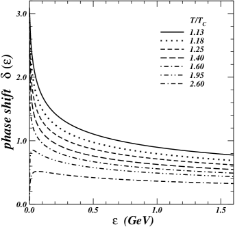
Figure 2: Phase shift as a function of the composite continuum energy $\epsilon$ and the plasma temperature calculated in the potential model using the $W_{1}({\bf r},T)$ potential.

When there are $m$ bound $S$ states in the potential, the $S$ wave phase shift at zero energy will start at $m\pi$, in accordance with the Levinson theorem. For the $W_{1}({\bf r},T)$ potential, there is one bound S-wave state for temperatures below $\sim$1.6$T_{c}$, as indicated by the phase shift of $\delta(\epsilon=0)$=$\pi$. The phase shift gradually decreases as energy increases and $\partial\delta(\epsilon)/\partial\epsilon$ is negative for all continuum energies. In this case with one or many $S$-wave bound states, the time delays for all continuum states are negative and there are no Gamow states in the continuum. Thus, in Eq. (49), only a single term, a bound state term with a bound state mass $M_{b}$, contributes to the correlator $G(\tau)$ for $T<\sim 1.6T_{c}$. The correlator $G(\tau)$ of Eq. (49) becomes

$$G(\tau)\propto\frac{\cosh\{M_{b}(T)(\tau-\beta/2)\}}{\sinh\{M_{b}(T)\beta/2)\}}$$ (67)

where $M_{b}(T)$ is the mass of the bound $S$ state at the temperature $T$. A lattice gauge correlator $G(\tau)$ is represented in terms of its ratio with respect to a “reconstructed” correlator $G_{\rm recon}(\tau)$, which is defined as the correlator calculated with the “reconstructed” spectrum at $T=0$. In actual practice in the evaluation of the lattice gauge correlators $G_{\rm recon}(\tau)$ to obtain the ratios of $G(\tau)/G_{\rm recon}(\tau)$ shown in Figs. 1a and 3a, Ref. Dat03 has used the “reconstructed” spectrum at $T=0.75T_{c}$ which contains only a single bound state footnote2 . Therefore, in order to compare with lattice gauge $G(\tau)/G_{\rm recon}(\tau)$, we need to include only a single lowest mass bound state in Eq. (49) to evaluate the “reconstructed” correlator $G_{\rm recon}(\tau)$ in the potential model. The potential model correlator $G(\tau)$ relative to the potential model $G_{\rm recon}(\tau)$, normalized to unity at $\tau=0$, is thus

$$\frac{G(\tau)}{G_{\rm recon}(\tau)}=a\frac{\cosh\{M_{b}(T)(\tau-\beta/2)\}}{\sinh\{M_{b}(T)\beta/2)\}}\Biggr{/}\frac{\cosh\{M_{b}(T=0)(\tau-\beta/2)\}}{\sinh\{M_{b}(T=0)\beta/2)\}},$$ (68)

where $a=\tanh(M_{b}(T)\beta/2)/\tanh(M_{b}(T=0)\beta/2)\sim 1$.

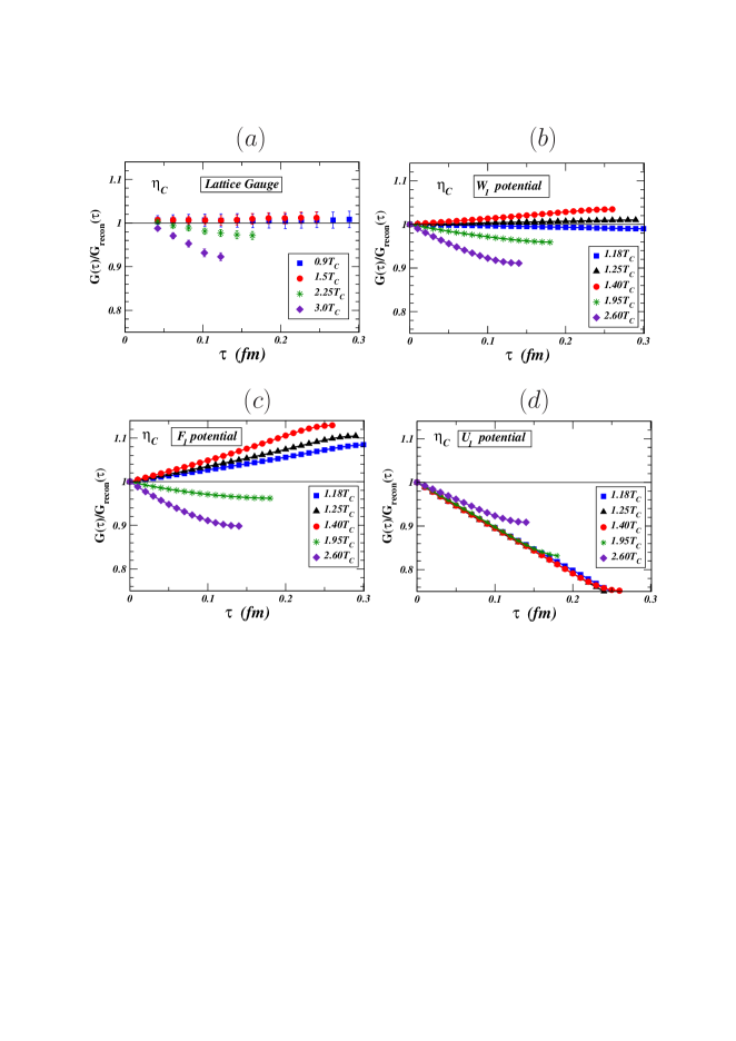
Figure 3: Fig. 3a shows the pseudoscalar charmonium correlators $G(\tau)/G_{\rm recon}(\tau)$ obtained in lattice gauge calculations Dat03 . The potential model pseudoscalar charmonium correlators $G(\tau)/G_{\rm recon}(\tau)$ obtained with the $W_{1}({\bf r},T)$ potential of Eq. (58) are shown in Fig. 3b, with the free energy $F_{1}({\bf r},T)$ potential in Fig. 3c, and with the internal energy energy $U_{1}({\bf r},T)$ potential in Fig.  3d.

Using the above equation that is based on the concept of the absence of $L$=0 resonance states and Gamow states when a bound state is present, we calculate the potential model correlators $G(\tau)/G_{\rm recon}(\tau)$ for the cases of 1.18$T_{c}$, 1.25$T_{c}$, and 1.40$T_{c}$ with bound state masses $M(T)$ obtained in the $W_{1}({\bf r},T)$ potential as given in Table I. The results for these three temperatures are shown in Fig. 3b. As the bound state mass values in Table I have uncertainties of about $\pm$0.7% in $M(T)$, the uncertainties of the potential model correlators are about $\pm 0.007$ in $G/G_{\rm recon}$. The potential model correlators can be compared with the correlators obtained in lattice gauge calculations show in Fig. 3a Dat03 . The general features of the potential model correlators at these three temperatures below about 1.6$T_{c}$ agree with those of the lattice gauge correlators. In particular, the slopes $d[G/G_{\rm recon}]/d\tau$ in Fig. 3b for $T<\sim 1.6T_{c}$ in potential model calculations are of the order $\sim 0.03-0.1/$fm, which do not differ much from the nearly zero slopes of $d[G/G_{\rm recon}]/d\tau$ in Fig. 3a for $T=0.9T_{c}$ and 1.5$T_{c}$ in lattice gauge calculations. They differ significantly from the general shapes of the potential model correlators obtained by the authors of Ref. Moc06 ; Moc06a in Figs. 1b and 1c, where $d[G/G_{\rm recon}]/d\tau\sim 1/$fm in Fig. 1b and $\sim 2.5/$fm in Fig. 1c, for $\tau<0.2$fm.

As the temperature increases above $\sim$1.6$T_{c}$, the $S$-wave state calculated with the $W_{1}({\bf r},T)$ potential is no longer bound and the phase shifts at $T/T_{c}=1.95$ and $2.60$ are shown in Fig. 2. For these cases without a bound $S$-wave state, the phase shift starts at zero at zero continuum energy $\epsilon$ and it increases rapidly as the energy increases. After reaching a peak value below $\pi/2$, the phase shift decreases slowly as the energy increases. Thus, there is a region of continuum states for which $\partial\delta(\epsilon)/\partial\epsilon$ is positive. They possess positive time delays and lifetimes. They are Gamow states capable of propagating as a composite meson to contribute to the meson correlator. In this case without an $S$-wave bound state, there are no contributions from bound states to the correlator $G(\tau)$. Only continuum Gamow states represented by the integral over ${\bf k}$ contribute to the meson correlator $G(\tau)$ in Eq. (49).

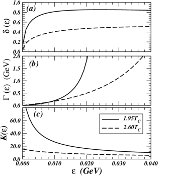
Figure 4: (Fig. 4a) The phase shift $\delta(\epsilon)$ as a function of the continuum energy $\epsilon$ at $T=1.95T_{c}$ and $2.6T_{c}$, calculated in the $W_{1}({\bf r},T)$ potential of Eq. (58). (Fig. 4b) The width of the Gamow states $\Gamma(\epsilon)$ as a function of the continuum energy $\epsilon$. (Fig. 4$c$) ${\cal K}(\epsilon)$ as a function of $\epsilon$.

An expanded view of the phase shift $\delta(\epsilon)$ as a function of the continuum state ${\bf k}$ with energy $\epsilon={\bf k}^{2}/2\mu_{m}$ is shown in Fig. 4a for $T=1.95T_{c}$ and $T=2.60T_{c}$. The corresponding width $\Gamma(\epsilon)$ extracted from the time delay $\partial\delta(\epsilon)/\partial\epsilon)$ is shown in 4b. At $T=1.95T_{c}$, the width is zero at $\epsilon$=0, and the gradual increase in width turns into a rapid increase as $\epsilon$ increases. The increase in width is less rapid at the higher temperature of 2.6$T_{c}$. Above the energy $\epsilon({\rm max})$ at which $\Gamma(\epsilon({\rm max}))=\Gamma_{\rm max}$ where $\Gamma_{\rm max}=2T$, the width of the continuum state is either too large or $\partial\delta(\epsilon)/\partial\epsilon$ is negative, and continuum states with energy above $\epsilon({\rm max})$ will not contribute to the meson correlator in the integral over ${\bf k}$. For $T=1.95T_{c}$, $\epsilon({\rm max})$ is 0.018GeV, and for $T=2.60T_{c}$, $\epsilon({\rm max})$ is 0.033GeV. They are located at energies slightly above the continuum threshold.

We can also evaluate the amplitude of the continuum wave function at the origin. The comparison of the absolute square of the amplitude at the origin ${\bf r}=0$, with the absolute square of the amplitude at very large ${\bf r}$ gives the ${\cal K}$-factor for the continuum state Won97 shown in Fig. 4c. This ${\cal K}$-factor is quite large at low energies, due to the attractive interaction between the quark and the antiquark. The ${\cal K}$-factor decreases as a function of the continuum energy $\epsilon$. We need to specify the width limit $\Gamma_{\rm max}(T)=1/\tau_{\rm min~{}life}(T)=2T$ by using Eq. (46). For $T=1.95T_{c}$, $\tau_{\rm min~{}life}$ is 0.185fm and $\Gamma_{\rm max}$ is 1.05GeV. For $T=2.6T_{c}$, $\tau_{\rm min~{}life}$ is $0.141$fm and $\Gamma_{\rm max}$ is 1.40GeV.

After setting the limit on the width of the Gamow states, we can calculate the pseudoscalar meson correlator, $G(\tau)/G_{\rm recon}(\tau)$ normalized to unity at $\tau=0$, for the case without a bound state. The results of the potential model correlators for $1.95T_{c}$ and $2.6T_{c}$ using the $W_{1}({\bf r},T)$ potential are shown in Fig. 3b. As one observes, the general trends of the correlators at these temperatures agree with those from the lattice gauge correlators.

The results in Figs. 3a and 3b indicate that when the contributions from bound states and continuum states are properly treated, there is indeed agreement between the lattice gauge correlators and the potential model correlators using the $W_{1}({\bf r},T)$ potential that is a linear combination of $F_{1}({\bf r},T)$ and $U_{1}({\bf r},T)$.

It is of great interest to investigate whether the potential model correlators depends on the potential. Accordingly, we evaluate the potential model correlators using the color-singlet free energy $F_{1}({\bf r},T)$ Dig01a ; Won01a ; Bla05 and the internal energy $U_{1}({\bf r},T)$ Kac02 ; Shu03 ; Alb05 ; Man05 for comparison. We need the bound state masses at various temperatures to evaluate the correlators, as required by Eqs. (49) and (68). We list state energy $\epsilon(T)$ and bound state mass $M(T)$ calculated in the $F_{1}({\bf r},T)$ potential and the $U_{1}({\bf r},T)$ potential for the $L$=0 charmonium in Table III.

Table III. Bound state energy $\epsilon(T)$ and bound state mass $M(T)$ (all in GeV) for the $L$=0 charmonium

calculated with the $F_{1}$ and $U_{1}$ potentials in quenched QCD.

$T$		1.13$T_{c}$	1.18$T_{c}$	1.25$T_{c}$	1.4$T_{c}$	1.6$T_{c}$	1.95$T_{c}$	2.60$T_{c}$
$F_{1}$ Potential	$\epsilon(T)$	-0.0117	-0.0051	-0.0018	-0.000007	unbound	unbound	unbound
	Mass $M(T)$	3.029	3.012	2.997	2.972
$U_{1}$ Potential	$\epsilon(T)$	-0.7483	-0.4422	-0.2613	-0.1331	-0.07820	-0.0669	-0.0225
	Mass $M(T)$	3.188	3.279	3.285	3.279	3.265	3.259	3.201

We note that as a function of temperature $T$, the $L=0$ charmonium masses with the $F_{1}$ potential are lower than the mass at $T=0$ and they decrease slowly with temperature up to its dissociation temperature at $\sim 1.4T_{c}$. On the other hand, for the $U_{1}$ potential the masses are greater than the charmonium mass at $T=0$ and vary only slightly with temperature.

We need to calculate further the phase shifts and the wave function amplitude at the origin and evaluate the correlators in these potential models. The potential model correlators obtained with $F_{1}$ and $U_{1}$ as the potentials are shown in Fig. 3c and 3d respectively. The comparison of these potential model correlators with the lattice gauge correlators indicates that the correlators calculated with the $F_{1}({\bf r},T)$ and $U_{1}({\bf r},T)$ potentials deviate from the lattice gauge correlators, the deviation being greater for the $U_{1}$ potential than the $F_{1}$ potential. The comparison shows that among the three different potentials, correlators obtained with the $W_{1}({\bf r},T)$ potential of Won05 ; Won05a ; Won06 ; Won06a give the best agreement with the lattice gauge correlators.

VIII Implications on the Lattice Gauge Spectral Function Analysis

The analysis of spectral function at finite temperatures in lattice gauge theory contains systematic uncertainties and lattice artifacts. In the maximum entropy method used for the spectral function analysis, it is necessary to assume a default spectrum to define the entropy. The spectral function obtained in the maximum entropy method depends on the assumed default spectrum (see Fig. 4 of Dat03 ). The extracted spectra often exhibit two prominent broad peaks in the continuum which do not seem to correspond to physical continuum states Asa03 ; Mat01 ; Dat03 ; Pet05 ; Jak06 . While it is important to study theoretically what the lattice artifacts are expected to be, some prior knowledge of the spectral function as inferred from the potential model will be useful to provide additional information for the assumed default spectrum and the expected spectral function.

From the physical picture that emerges in the evaluation of the current-current correlator, the spectral function analysis in the lattice gauge theory should be guided by the basic principle that out of the set of continuum states, only resonance states and Gamow states with lifetimes of sufficient magnitudes can propagate as composite objects and can contribute to the current-current correlator. The potential model can provide useful information on the nature of bound states, resonance states, and Gamow states for spectral function analysis. We can discuss first the case of $L=0$. As the $Q$-$\bar{Q}$ interaction itself does not possess a barrier, we expect that there are no $L=0$ potential resonances in the continuum New66 . The occurrence of $L=0$ bound states in the potential is accompanied by phase shifts with negative $\partial\delta(\epsilon)/\partial\epsilon$ (Fig. 2) with no delay time and composite lifetime for the continuum states. Consequently when $L=0$ bound states occur, only bound states can contribute to the correlator. According to these results of the potential model, the lattice gauge spectral function analysis for $L=0$ states should include only bound states without continuum states. On the other hand, when the $L=0$ bound states are absent, states with delay time and widths occurs at energies close to $\epsilon\sim 0$. The correlator receives contribution only from this region of continuum states (see Fig. 3b) and lattice gauge spectrum function analysis for $L=0$ states should employ a default spectrum that contains this element of the continuum contribution.

For the case of $L>0$, the presence of centrifugal barrier leads to potential pockets and possible potential resonance states, which may or may not occur, depending on the strength of the potential and the centrifugal barrier. One expects that when potential resonance states occur, the phase shift decreases as a function of $\epsilon$ at continuum energies above the resonance energies, and only bound states and possible resonance states contribute to the correlator in lattice gauge analysis. On the other hand, when bound states and resonance states are absent (as for example at high temperatures), Gamow states with delay time and widths of various magnitude occurs. The correlator receives contribution only from these Gamow states. Lattice gauge spectrum function analysis for $L>0$ states should employ a default spectrum that contains these essential characteristics.

IX Conclusions and Discussions

The potential model has been a useful concept in the physics of heavy quarkonia since the discovery of $J/\psi$. It provides a useful tool to examine quarkonium energies, quarkonium wave functions, reaction rates, transition rates, and decay widths God85 ; Bar92 ; Won02 ; Cra04 ; Cra06 . It allows the extrapolation to the region of high temperatures by expressing screening effects in terms of the temperature dependence of the potential Mat86 ; Dig01a ; Won01a ; Kac02 ; Shu03 ; Won05 ; Won05a ; Won06 ; Won06a ; Son05 ; Alb05 ; Bla05 ; Man05 ; Dig05 . The comparisons of the potential model dissociation temperatures with the lattice gauge spectral function dissociation temperatures show consistency when one uses the potential that is a linear combination of the free energy and the internal energy proposed in Won05 ; Won05a .

In addition to lattice gauge spectral function analyses, results have also been obtained for the lattice gauge current-current correlators Moc06 ; Moc06a . The current-current correlator is related to the spectral function by a generalized Laplace transform. In principle, they carry equivalent information. One expects that the consistency of the potential model with lattice gauge spectral function analyses should be extended to the comparison of the potential model current-current correlators with lattice gauge current-current correlators. Recent works in Refs. Moc06 ; Moc06a however make the contrary claim that the meson correlators obtained from many different types of potential models are not consistent with lattice gauge correlators and potential models cannot describe heavy quarkonia above $T_{c}$. In the work of Ref. Moc06 ; Moc06a , continuum states arising from a free fermion $Q$ and $\bar{Q}$ pair in a fermion gas contribute to the correlator. However, to be able to propagate as a composite meson so as to contribute to the correlator, the quark and antiquark must be temporally and spatially correlated. Continuum states in the free quark and antiquark gas may not have sufficient temporal and spatial correlations to qualify as composite objects for such a propagation.

Following the basic principle that among the continuum states only resonance states and Gamow states with a lifetime of sufficient magnitude can propagate as a composite object and contribute to the correlator, we re-evaluate the current-current correlator in the potential model. With the simple example of the pseudoscalar correlator, we show in this paper that when the bound state and continuum state contributions are properly treated, the $W_{1}({\bf r},T)$ potential using a linear combination of $F_{1}$ and $U_{1}$ proposed in Won05 ; Won05a gives correlators consistent with those of lattice gauge correlators, while the $F_{1}$ potential and the $U_{1}$ potential lead to deviations. Our results indicate consistency of the $W_{1}({\bf r},T)$ potential proposed in Won05 ; Won05a with both the lattice gauge spectral function analysis and the lattice gauge correlator analysis. The present agreement is not surprising as the current-current correlator and the spectral function are related by a generalized Laplace transform, and they indeed carry equivalent information.

There are uncertainties, limitations, and future prospects in the potential model that requires further investigations. Lattice gauge calculations provide information on thermodynamical quantities of the free energy $F_{1}$ and the internal energy $U_{1}$. We have shown deductively in Eq. (11) of Ref. Won05 that the internal energy $U_{1}({\bf r},T)$ contains $U_{Q\bar{Q}}^{(1)}({\bf r},T)$ and $U_{g}^{(1)}({\bf r},T)-U_{g0}(T)$. Only $U_{Q\bar{Q}}^{(1)}({\bf r},T)$ pertains to the interaction potential between $Q$ and $\bar{Q}$. The other parts need to be subtracted out from $U_{1}({\bf r},T)$ to obtain the $Q$-$\bar{Q}$ potential. We have made use of the knowledge of the equation of state from an independent lattice gauge calculations to evaluate $U_{Q\bar{Q}}^{(1)}({\bf r},T)$ from $U_{1}({\bf r},T)$, leading to the present linear-combination model of the $U_{Q\bar{Q}}^{(1)}({\bf r},T)$ potential of Eq. (58). However, a more rigorous treatment will involve a direct evaluation of the $Q$-$\bar{Q}$ potential by evaluating the quantities of $U_{g}^{(1)}({\bf r},T)-U_{g0}(T)$ in the lattice gauge theory. It will be of great interest to examine how one can determine directly the $Q$-$\bar{Q}$ potential in a lattice gauge calculations without resort to the equation of state.

The potential model we have developed so far has the limitation that the important spin-spin interaction has not been included. As the spin-spin interaction is responsible for the $\eta_{c}$-$J/\psi$ and $\eta_{b}$-$\Upsilon$ splittings, it modifies the binding energies and the dissociation temperatures. It is important to include spin-spin and other components of the $Q$-$\bar{Q}$ interactions in the potential model to see how they may affect the stability of heavy quarkonia.

The potential model allows the evaluation of many quantities of interest. The potential model in the present manuscript uses thermodynamical quantities obtained in quenched QCD. The effects of dynamical quarks on the stability of quarkonia can be studied by using potential models extracted from thermodynamic quantities calculated in full QCD Kac05 ; Won05a . One can examine the quark mass dependence of quarkonium stability and quarkonium gluon dissociation cross sections, some results of which have been presented recently Won06 ; Won06a . The heavy quark potential model so far developed has the limitation that it is restricted to non-relativistic cases. It will also be of interest to study the relativistic effects by examining relativistic two-body potential models along the lines of Dirac’s constraint dynamics as in Ref. Cra04 ; Cra06 , which will allow us to study the stability of light-quark systems within the potential model.

After the present manuscript has been submitted for publication, a recent preprint Alb06 refers to our procedure of including only states of sufficient lifetimes and asserts that “this procedure might be incorrect, since the evaluated correlator has to be compared with the lattice ones, which do have a free gas (infinite temperature) limit.”

This statement in Ref. Alb06 with regard to our work might be incorrect. Firstly, the evaluated lattice gauge correlators of Ref. Dat03 to be compared were carried out in finite temperatures with $T\sim(1-3)T_{c}$ and $T<<T_{\infty}$ ($T_{\infty}\to\infty)$. This temperature $T$ is in the non-perturbative region and is far from the infinite temperature perturbative QCD limit. The spectrum of a free gas pQCD limit at infinite temperature is not relevant to the finite temperature lattice gauge correlators being compared at hand. Secondly, the presence of a continuum spectrum in the infinite temperature limit is in fact consistent with our procedure of including states of sufficient lifetimes at that infinite temperature limit.

The arguments to support our procedure have been presented already in the manuscript. We repeat the main points again below to rebut the statement of Alb06 .

As discussed in Eq. (1), the meson correlator describes the probability amplitude for creating a composite meson at time 0 and subsequently destroying the composite meson at time $\tau$. The operation of destroying the meson at time $\tau$ can be considered as an operation of measurement (or an operation of detection) of the meson at time $\tau$. From the discussions in Eqs. (28) and (29), $\tau$ is less than and up to $\beta/2$ or $1/2T$, where $T$ is the temperature, and the measurement operation takes place within $\tau<1/2T$. At the temperature $T$, in order to be detected by the correlator measurement at $\tau=1/2T$, the composite meson state needs to have a lifetime $\tau_{\rm life}$ greater than $1/2T$, which has been conveniently labeled as $\tau_{\rm min~{}life}(T)=1/2T$ in Eq. (45), the minimum meson state lifetime (for correlator detection) at temperature $T$.

From this analysis, the composite meson states that can be detected by the correlator measurement will include meson states of shorter and shorter lifetimes as temperature increases, and the correlator spectrum above the bound states region will depend on the temperature. In the infinite temperature limit $T=T_{\infty}\to\infty$, the minimum lifetime $\tau_{\rm min~{}life}(T_{\infty})$, which is equal to $1/2T_{\infty}$, approaches zero. The correlator measurement includes states that live for a very short composite object lifetime $\tau_{\rm life}>\tau_{\rm min~{}life}(T_{\infty})\sim 0$. This condition can be satisfied for weakly interacting free gas continuum states. The correlator allows a free gas continuum spectrum in the infinite temperature limit. The presence of a continuum spectrum in the infinite temperature limit is consistent with our procedure of including states of sufficient lifetimes.

We turn our attention now to the finite-temperature lattice gauge calculations in Ref. [24] with $T\sim(1-3)T_{c}$ and $T<<T_{\infty}$. Our afore-mentioned comparison of the meson lifetime and the minimum lifetime for the correlator measurement indicates that only composite states that have lifetimes $\tau_{\rm life}$ greater than $\tau_{\rm min~{}life}(T)=1/2T$ can survive and be detected by the correlator measurement at $T$. Free gas continuum states with very short composite object lifetimes $\tau_{\rm min~{}life}(T_{\infty})=1/2T_{\infty}$, much smaller than $\tau_{\rm min~{}life}(T)=1/2T$, cannot survive up to $\tau_{\rm min~{}life}(T)=1/2T$ and will not be detected by the correlator measurement at $T$. Because of this limitation, the meson spectrum obtained in finite-temperature correlator calculations at $T$ should be different from the correlators in the infinite temperature limit and should only contain bound states, resonance states, and Gamow states of sufficient lifetimes greater than $1/2T$.

Based on the above rebuttal, there might be no basis for the authors in Ref. Alb06 to make the statement mentioned above.

In conclusion, we have found that the potential model of Ref. Won05 is consistent with both spectral function analyses and current-current correlator analyses. The potential model of Won05 can be a useful tool to complement lattice gauge calculations for the study of heavy quarkonia at high temperatures.

This research was supported in part by the Division of Nuclear Physics, U.S. Department of Energy, under Contract No. DE-AC05-00OR22725, managed by UT-Battle, LLC and by the National Science Foundation under contract NSF-Phy-0244786 at the University of Tennessee and Contract No. NSF-PHY-0244819 at the University of Tennessee Space Institute.

References

- (1) S. Godfrey and N. Isgur, Phys. Rev. D32, 189 (1985).
- (2) T. Barnes and E. S. Swanson, Phys. Rev. D46, 131 (1992).
- (3) C. Y. Wong, T. Barnes and E. S. Swanson, Phys. Rev. C65, 014903 (2002).
- (4) H. W. Crater and P. Van Alstine, Phys. Rev. D70, 034026, (2004).
- (5) H. W. Crater, C. Y. Wong, and P. Van Alstine, Phys. Rev. D74, 054028 (2006).
- (6) T. Matsui and H. Satz, Phys. Lett. B178, 416 (1986).
- (7) S. Digal, P. Petreczky, and H. Satz, Phys. Lett. B514, 57 (2001); Phys. Rev. D64, 094015 (2001).
- (8) C. Y. Wong, Phys. Rev. C 65, 034902 (2002); J. Phys. G28, 2349 (2002).
- (9) O. Kaczmarek, F. Karsch, and P. Petreczky, and F. Zantow, Phys. Lett. B543, 41 (2002); F. Zantow, O. Kaczmarek, F. Karsch, and P. Petreczky, hep-lat/0301015.
- (10) E. V. Shuryak and I. Zahed, Phys. Rev. C70 , 021901 (2004); Phys. Rev. D70, 054507 (2004); E. V. Shuryak, Nucl. Phys. A750, 64 (2005).
- (11) C. Y. Wong, Phys. Rev. C72, 034906 (2005).
- (12) C. Y. Wong, hep-ph/0509088. talk presented at Recontre de Blois, Chateau de Blois, France, May 15-20, 2005.
- (13) C. Y. Wong, J. Phys. G32, S301 (2006), [hep-ph/060614].
- (14) C. Y. Wong, hep-ph/0606200.
- (15) T. Song and S. H. Lee, Phys. Rev. D 72, 034002 (2005).
- (16) W.M. Alberico, A. Beraudo, A. De Pace, and A. Molinari, hep-ph/0507084;
- (17) D. Blaschke, O. Kaczmarek, E. Laermann, and V. Yudichev, Eur. Phys. J. C43, 81 (2005).
- (18) M. Mannarelli and R. Rapp, Physical Review C72, 064905 (2005).
- (19) S. Digal, O. Kaczmarek, F. Karsch, and H. Satz, Eur. Phys. J. C43, 71 (2005).
- (20) A. Mocsy and P. Petreczky, Phys. Rev. D73, 074007 (2006).
- (21) A. Mocsy and P. Petreczky, hep-ph/0606053.
- (22) M. Asakawa, T. Hatsuda, and Y. Nakahara Nucl. Phys. A715, 863 (2003); M. Asakawa and T. Hatsuda, Phys. Rev. Lett. 92, 012001 (2004); M. Asakawa, T. Hatsuda, Y. Nakahara, Prog. Part. Nucl. Phys. 46, 459 (2001); T. Hatsuda, hep-ph/0509306.
- (23) H. Matsufuru, T. Onogi, and T. Umeda, Phys. Rev. D64, 114503 (2001).
- (24) S. Datta, F. Karsch, P. Petreczky, and I. Wetzorke, Phys. Rev. D69 , 094507 (2004), and J. Phys. G31, S351 (2005).
- (25) K. Petrov, Eur. Phys. J. C43, 67 (2005); A. Mocsy, Talk presented at Quark Matter Conference, 2005, hep-ph/0510135; P. Petreczky, Talk presented at Quark Matter Conference, 2005.
- (26) A. Jakovác, P. Petreczky, K. Petrov, and A. Velytsky, hep-lat/0611017.
- (27) O. Kaczmarek, F. Karsch, P. Petreczky, and F. Zantow hep-lat/0309121.
- (28) O. Kaczmarek and F. Zantow, Phys. Rev. D71, 114510 (2005), and O. Kaczmarek and F. Zantow, hep-lat/0506019.
- (29) A Gamow state as well as a resonance state is a state with a finite lifetime. For the case of an interacting two-body system, a resonance state is further characterized by a phase shift of where is an integer, and .
- (30) F. Karsch, M. G. Mustafa, and M. H. Thoma, Phys. Lett. B497, 249 (2001).
- (31) To reconstruct the quantity in lattice gauge calculations, Ref. Dat03 actually used the quarkonium spectrum at (Fig. 2 of Dat03 ) obtained in the spectral function analysis. As shown in Fig. 2 of Ref. Dat03 , the spectrum at contains only a single bound state peak in the bound state energy region.
- (32) D. L. Tubbs and S. E. Koonin, Astrophys. J. 232, L59 (1979).
- (33) S. Shlomo, Nucl. Phys. A539, 17 (1992); S. Shlomo and J. B. Natowitz, Phys. Lett. B252, 187 (1990).
- (34) S. Shlomo and G. F. Bertsch, Nucl. Phys. A243, 507 (1995).
- (35) S. Shlomo, V. M. Kolomietz, and H. Dejbakhsh, Phys. Rev. C55, 1972 (1997).
- (36) R. J. Charity and L. G. Sobotka, Phys. Rev. C 71, 024310 (2005).
- (37) Y. Alhassid, G. F. Bertsch, and L. Fang, Phys. Rev. C68, 044322 (2003).
- (38) C. Y. Wong and H. Crater, Phys. Rev. C63, 044907 (2001).
- (39) L. P. Kadanoff and G. Baym, Quantum Statistical Mechanics, W. A. Benjamin, Inc, Reading, Mass. 1962.
- (40) E. Wigner, Phys. Rev. 98, 145 (1967).
- (41) R. G. Newton, Scattering Theory of Waves and particles, Dover Publications, 1966, p. 314;
- (42) A. deShalit and H. Feshbach, Theoretical Nuclear Physics, Volume I, Nuclear Structure, J. Wiley, N.Y. 1974, p. 88.
- (43) G. R. Satchler, Introduction to Nuclear Reactions, Oxford University Press, 1990, p. 235;
- (44) K. W. McVoy, Annals of Phys. (N.Y.), 43, 91 (1967).
- (45) C. Y. Wong and L. Chatterjee, Zeit. Phys. C75, 523 (1997).
- (46) G. Boyd , Nucl. Phys. B 469, 419 (1996)
- (47) J. A. Wheeler, Phys. Rev. 52, 1123 (1937).
- (48) F. Calogero, Variable Phase Approach to Potential Scattering, Academic Press, N.Y. 1967.
- (49) W. M. Alberico, A. Beraudo, A. De Pace, and A. Molinari, hep-ph/0612062.