Abstract

We confront a very wide body of HERA diffractive electroproduction data with the predictions of the colour dipole model. In doing so we focus upon three different parameterisations of the dipole scattering cross-section, whose parameters are fixed by analysis of DIS structure function data. This analysis strongly suggests the presence of saturation effects, but is not definitive because the conclusion requires the inclusion of data at low-$Q^{2}$ values.

Having fixed the parameters of the models from the DIS structure function data, the resulting dipole cross sections can be used to make genuine predictions for other reactions. Good agreement is obtained for all observables, as is illustrated here for deeply virtual Compton scattering(DVCS) and diffractive deep inelastic scattering(DDIS). There can be no doubting the success of the dipole scattering approach and more precise observations are needed in order to expose its limitations

1 Introduction

In the colour dipole model  [3, 4], the forward amplitude for virtual Compton scattering is assumed to be dominated by the mechanism illustrated in Fig.1 in which the photon fluctuates into a $q\bar{q}$ pair of fixed transverse separation $r$ and the quark carries a fraction $z$ of the incoming photon light-cone energy. Using the Optical Theorem, this leads to

$$\sigma_{\gamma^{\ast}p}^{L,T}=\int dz\;d^{2}r\ |\Psi_{\gamma}^{L,T}(r,z,Q^{2})|^{2}\sigma(s^{\ast},r)$$ (1)

for the total virtual photon-proton cross-section, where $\Psi_{\gamma}^{L,T}$ are the appropriate spin-averaged light-cone wavefunctions of the photon and $\sigma(s^{\ast},r)$ is the dipole cross-section. The dipole cross-section is usually assumed to be independent of $z$, and is parameterised in terms of an energy variable $s^{\ast}$ which depends upon the model.

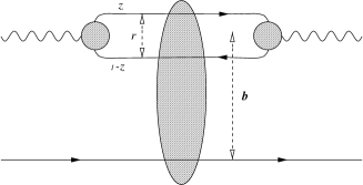
Figure 1: The colour dipole model for elastic Compton scattering $\gamma^{\ast}p\rightarrow\gamma^{\ast}p$.

Thus using Eq.(1) we are able to compute the deep inelastic structure function $F_{2}(x,Q^{2})$. The power of the dipole model formulation lies in the fact that the same dipole cross-section $\sigma(s^{*},r)$ appears in a variety of other observables which involve the scattering of a real or virtual photon off a hadronic (or nuclear) target at high centre-of-mass (CM) energy. The largeness of the CM energy guarantees the factorization of scattering amplitudes into a product of wavefunctions and a universal dipole cross-section. In this paper we wish to test the universality of the dipole cross-section using a wide range of high quality data collected at the HERA $ep$ collider. Moreover, we also wish to examine the extent to which to data are able to inform us of the role, if any, played by non-linear saturation dynamics.

2 The dipole cross-section

We now turn to the three different models used to describe the dipole cross-section. Before doing so however, we shall first discuss our choice of photon wavefunction. For small $r$, the light-cone photon wavefunctions are given by the tree level QED expressions [3].

These wavefunctions decay exponentially at large $r$, with typical $r$-values of order $Q^{-1}$ at large $Q^{2}$ and of order $m_{f}^{-1}$ at $Q^{2}=0$. However for large dipoles $r\approx 1$ fm, which are important at low $Q^{2}$, a perturbative treatment is not really appropriate. In this region some authors [5] modify the perturbative wavefunction by an enhancement factor motivated by generalised vector dominance (GVD) ideas [6, 7, 8], while others [9] achieve a similar but broader enhancement by varying the quark mass. In practice [1], the difference between these two approaches only becomes important when analysing the precise real photoabsorption data from fixed-target experiments [11]. Since we will not consider these data here, we will adopt the simpler practise of using a perturbative wavefunction at all $r$-values, and adjusting the quark mass to fit the data.

Turning now to the dipole cross-section, all three models are consistent with the physics of colour transparency for small dipoles and exhibit soft hadronic behaviour for large dipoles. As stated above, the model parameters are determined by fitting only to the DIS structure function data. Since the details of all three models have been published elsewhere, we shall here summarise their properties only rather briefly.

2.1 The FS04 Regge model [1]

This simple model, due to Forshaw and Shaw [1], combines colour transparency for small dipoles $r<r_{0}$ with “soft pomeron” behaviour for large dipoles $r>r_{1}$ by assuming

$$\sigma(x_{m},r) =A_{H}r^{2}x_{m}^{-\lambda_{H}}~{}~{}{\mathrm{for}}~{}~{}r<r_{0}~{}~{}{\mathrm{and}}$$

$$=A_{S}x_{m}^{-\lambda_{S}}~{}~{}{\mathrm{for}}~{}~{}r>r_{1},$$ (2)

where $x_{m}=(Q^{2}+4m_{f}^{2})/(Q^{2}+W^{2})\,.$ For light quark dipoles, the quark mass $m_{f}$ is a parameter in the fit, whilst for charm quark dipoles the mass is fixed at 1.4 GeV. In the intermediate region $r_{0}\leq r\leq r_{1}$, the dipole cross-section is given by interpolating linearly between the two forms of Eq.(2).

If the boundary parameters $r_{0}$ and $r_{1}$ are kept constant then this parameterisation reduces to a sum of two powers, as might be predicted in a two pomeron approach, and can be thought of as an update of the original FKS Regge model [5] to accommodate the latest data. It is plainly unsaturated, in that the dipole cross-section obtained at small $r$-values and fixed $Q^{2}$ grows rapidly with increasing $s$ (or equivalently with decreasing $x$) without damping of any kind.

2.2 The FS04 Saturation model [1]

Saturation can be introduced into the above model by adopting a method previously utilised in [12]. Instead of taking $r_{0}$ to be constant, it is fixed to be the value at which the hard component is some specified fraction of the soft component, i.e.

$$\sigma(x_{m},r_{0})/\sigma(x_{m},r_{1})=f$$ (3)

and $f$ instead of $r_{0}$ is treated as a parameter in the fit. This introduces no new parameters compared to the Regge model. However, the scale $r_{0}$ now moves to lower values as $x$ decreases, and the rapid growth of the dipole cross-section at a fixed, small value of $r$ begins to be damped as soon as $r_{0}$ becomes smaller than $r$. In this sense we model saturation, albeit crudely, with $r_{0}$ the saturation radius.

2.3 The CGC saturation model [13]

In addition we shall consider the CGC dipole model originally presented by Iancu, Itakura and Munier [13]. This model aims to include the main features of the “Colour Glass Condensate” regime, and can be thought of as a more sophisticated version of the original “Saturation Model” of Golec-Biernat and Wüsthoff [9]. The original Iancu et al dipole cross-section was obtained using a three flavour fit to the DIS data Here we use a new four-flavour CGC fit due to Kowalski, Motyka and Watt [14].

3 Structure function data

The parameters of the FS04 models were determined by fitting the recent ZEUS $F_{2}$ data [15] in the kinematic range

$$0.045\,\mathrm{GeV}^{2}<Q^{2}<45\,\mathrm{GeV}^{2}\hskip 14.22636ptx\leq 0.01\;$$ (4)

whilst the CGC fit of [14] is to data with $Q^{2}>0.25$ GeV² (the other limits are as for FS04). The corresponding H1 data [16] could also be used, but it would then be necessary to float the relative normalisation of the two data sets. We do not do this since the ZEUS data alone suffice. The resulting parameter values are tabulated in the original papers; we do not reproduce them here, but confine ourselves to some general comments.

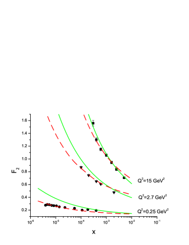
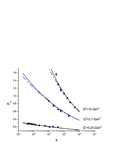
Figure 2: Comparison of our new dipole model fits to a subset of DIS data [15]. Left: No saturation fits. FS2004 Regge dipole fit (dashed line) and (solid line) a fit of the same model to data in the restricted range $5\times 10^{-4}<x<10^{-2}$, extrapolated over the whole $x$-range $x<0.01$. Right: Saturation fits. FS2004 saturation fit (solid line) and the CGC dipole model (dot-dashed line)

The best fit obtained with the FS2004 Regge model is shown as the dashed line in Figure 2 (left). As can be seen, the quality of the fit is not good, corresponding to a $\chi^{2}$/data point of 428/156. This is not just a failing of this particular parameterisation. We have attempted to fit the data with many other Regge inspired models, including the original FKS parameterizations [5, 19], without success.

A possible reason for this failing is suggested by the solid curve in Figure 2 (left), which shows a the result of fitting only to data in the $x$-range $5\times 10^{-4}<x<10^{-2}$, and then extrapolating the fit to lower $x$ values, corresponding to higher energies at fixed $Q^{2}$. As can be seen, this leads to a much steeper dependence at these lower $x$-values(i.e. at higher energies) than is allowed by the data at all $Q^{2}$. An obvious way to solve this problem is by introducing saturation at high energies, to dampen this rise. This is confirmed by fitting with the the FS04 saturation model, which yields a $\chi^{2}$/data point of 155/156. The resulting fit is shown in Figure 2 (right), which also shows the very similar results previously obtained using the more sophisticated CGC model.

It is clear from these results that the introduction of saturation into the model immediately removes the tension between the soft and hard components which is so disfavoured by the data. However, it is important to note that this conclusion relies on the inclusion of the data in the low $Q^{2}$ region: both the Regge and saturation models yield satisfactory fits if we restrict to $Q^{2}\geq 2\,{\rm GeV}^{2}$, with $\chi^{2}$/data point values of 78/86 and 68/86 respectively.

At this point we have three well-determined parameterisations of the colour dipole cross-section, which have been used by Forshaw, Sandapen and Shaw [2] to yield predictions for other processes. In the next sections we shall take a look at the results for Deeply Virtual Compton Scattering (DVCS) and the diffractive structure function $F_{2}^{D(3)}$ .We always choose to show the Regge fit, even though it does not fit the $F_{2}$ data particularly well, in order to indicate the discriminatory power of the data. We stress that in all cases, the photon wavefunctions and dipole cross-sections are precisely those determined from the fits to $F_{2}$ data, without any adjustment of parameters.

4 Deeply virtual Compton scattering

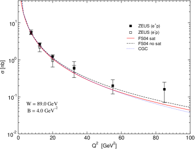
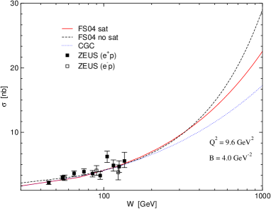
Figure 3: Comparison of the ZEUS DVCS data [21] with the predictions of the three models discussed in the text. Left : $Q^{2}$ dependence at $W=89$ GeV. Right: $W$ dependence at $Q^{2}=9.6$ GeV².

In deeply virtual Compton scattering, $\gamma^{\ast}+p\rightarrow\gamma+p$, the final state particle is a real as opposed to a virtual photon and dipole models provide predictions for the imaginary part of the forward amplitude with no adjustable parameters beyond those used to describe DIS. To calculate the forward cross-section a correction for the contribution of the real part of the amplitude has to be included. This correction was estimated in [19] and found to be less than $\approx 10\%$ and of a similar size in different dipole models. Predictions for the measured total cross-sections are then obtained using

$$\sigma_{L,T}(\gamma^{\ast}p\rightarrow\gamma p)=\frac{1}{B}\left.\frac{d\sigma^{T,L}}{dt}\right|_{t=0}\;,$$ (5)

where the value of the slope parameter $B$ is taken from experiment.

The predictions of all three dipole models are compared with the ZEUS data [21] in Fig.3, where we take a fixed value $B=4$ GeV^-2 which is compatible with their data. Bearing in mind this normalisation uncertainty, the agreement is good for all three models, although significant differences between the models appear when the predictions are extrapolated to high enough energies, as one would expect. Similarly good agreement is found for the H1 data [22] (see [2]).

5 Diffractive deep inelastic scattering (DDIS)

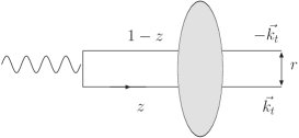
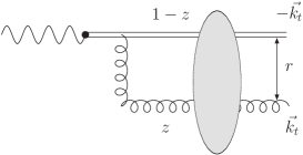
Figure 4: The $q\bar{q}$ and $q\bar{q}g$ contributions to DDIS.

To conclude our study we turn to the diffractive deep inelastic scattering (DDIS) process

$$\gamma^{\ast}+p\rightarrow X+p\;\;,$$

where the hadronic state $X$ is separated from the proton by a rapidity gap. In this process, in addition to the usual variables $x$ and $Q^{2}$ there is a third variable $M_{X}^{2}$. In practice, $x$ and $M_{X}^{2}$ are often replaced by the variables $x_{I\!\!P}$ and $\beta$:

$$x_{I\!\!P}\simeq\frac{M_{X}^{2}+Q^{2}}{W^{2}+Q^{2}}\hskip 28.45274pt\beta=\frac{x}{x_{I\!\!P}}\simeq\frac{Q^{2}}{M_{X}^{2}+Q^{2}}~{}.$$ (6)

In the diffractive limit $s\gg Q^{2},m_{X}^{2}$ and so $x_{I\!\!P}\ll 1$.

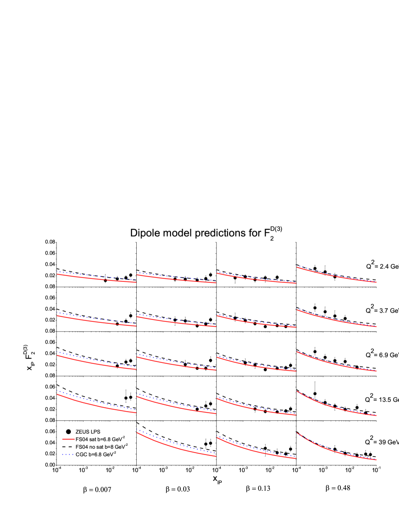
Figure 5: Model predictions compared to the ZEUS LPS data [25].

In the dipole model, the contribution due to quark-antiquark dipoles to the structure function $F_{2}^{D(3)}$ can be obtained from a momentum space treatment as described in [23, 9]. However, if we are to confront the data at low values of $\beta$, corresponding to large invariant masses $M_{X}$, it is necessary also to include a contribution from the higher Fock state $q\bar{q}g$. We can estimate this contribution using an effective “two-gluon dipole” approximation due to Wüsthoff [23], as illustrated in Fig.4.

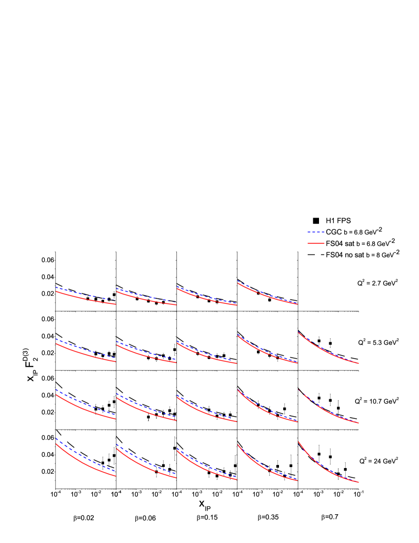
Figure 6: Model predictions compared to the H1 FPS data: $x_{I\!\!P}$ dependence [24].

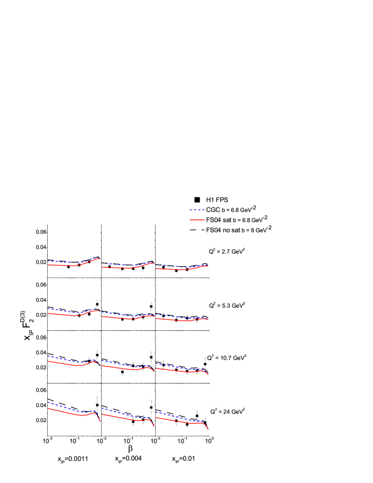
Figure 7: Model predictions compared to the H1 FPS data: $\beta$ dependence [24].

Again, the predictions obtained in this way involve no adjustment of the dipole cross-sections and photon wavefunctions used to describe the $F_{2}$ data. We are however free to adjust the forward slope for inclusive diffraction ($B$) within the range acceptable to experiment, which means that the overall normalisation, but not the energy dependence, of $F_{2}^{D(3)}$ is free to vary somewhat. We take $B=6.8$ GeV^-2 when making our CGC and FS04 saturation predictions and $B=8.0$ GeV^-2 when making the FS04 Regge predictions. Note that a value of $8.0$ GeV^-2 is rather high compared to the $\approx 6$ GeV^-2 favoured by the H1 FPS data [24] although it is in the range allowed by the ZEUS LPS data [25]. The need for a larger value of $B$ for the FS04 Regge model arises since the corresponding dipole cross-section is significantly larger than the FS04 saturation model at large values of $r$ and this enhancment is magnified in inclusive diffraction since it is sensitive to the square of the dipole cross-section. We should also bear in mind that the tagged proton data are subject to an overall $\approx 10\%$ normalisation uncertainty. We are also somewhat free to vary the value of $\alpha_{s}$ used to define the normalisation of the model dependent $q\bar{q}g$ component, which is important at low values of $\beta$. Rather arbitrarily we take $\alpha_{s}=0.1$ and take the view that the theory curves are less certain in the low $\beta$ region.

In Fig.5 we compare the recent ZEUS LPS data [25] on the $x_{I\!\!P}$ dependence of the structure function $F_{2}^{D(3)}$ at various fixed $Q^{2}$ and $\beta$ with the models. The agreement is good except at the larger $x_{I\!\!P}$ values. Indeed, the $\chi^{2}$ values per data point are very close to unity for all three models for $x_{I\!\!P}<0.01$. Disagreement at larger $x_{I\!\!P}$ is to be expected since this is the region where we anticipate a significant non-diffractive contribution which is absent in the dipole model prediction. Note that the three models produce similar predictions at larger values of $\beta$.

Comparison to the H1 data with tagged protons [24] is to be found in Fig.6 and Fig.7. The story is similar to that for the ZEUS data and the evidence for an overshoot of the CGC and Regge model predictions at low $\beta$ is strengthened. The $Q^{2}=2.7$ GeV² panes in Fig.7 illustrate this point the best. Again, we should not interpret this as evidence against these dipole models due to the uncertainty in the $q\bar{q}g$ contribution in the low $\beta$ region. The agreement between all models and the data at larger values of $\beta$ and low enough $x_{I\!\!P}$ is satisfactory..

In summary, the DDIS data at large enough $\beta\geq 0.4$ and small enough $x_{I\!\!P}\leq 0.01$ are consistent with the predictions of all three dipole models. However the data themselves would have a much greater power to discriminate between models if the forward slope parameter were measured to better accuracy. At smaller values of $\beta$, the data clearly reveal the presence of higher mass diffractive states which can be estimated via the inclusion of a $q\bar{q}g$ component in the dipole model calculation under the assumption that the three-parton system interacts as a single dipole according to the universal dipole cross-section. The theoretical calculation at low $\beta$ must be improved before the data in the region can be utilised to disentangle the physics of the dipole cross-section. Nevertheless, it is re-assuring to observe the broad agreement between theory and data in the low $\beta$ region.

6 Conclusion

The dipole scattering approach, when applied to diffractive electroproduction processes, clearly works very well indeed. The HERA data now constitute a large body of data which is typically accurate to the 10% level or better, and without exception the dipole model is able to explain the data in terms of a single universal dipole scattering cross-section. Perhaps the most important question to ask of the data is the extent to which saturation dynamics is present. Although the $F_{2}$ data suggest the presence of saturation dynamics [1], the remaining data on exclusive processes and on $F_{2}^{D(3)}$ are unable to distinguish between the models we consider here: these data are therefore unable to offer additional information on the possible role of saturation. We do note that a more accurate determination of the forward slope parameter in diffractive photo/electro-production processes would significantly enhance the impact of the data. However, it is hard to avoid the conclusion that only with more precise data or with data out to larger values of the centre-of-mass energy will we have the chance to make a definitive statement on the role of saturation without the inclusion of the low $Q^{2}$ $F_{2}(x,Q^{2})$ data in the analysis.

References

- [1] J.R. Forshaw and G. Shaw JHEP 0412 (2004) 052.
- [2] J. R. Forshaw, R. Sandapen and G. Shaw, hep-ph0608161, JHEP (in press).
- [3] N.N. Nikolaev and B.G. Zakharov, Z. Phys. C49 (1991) 607; C53 (1992) 331.
- [4] A.H. Mueller, Nucl. Phys. B415 (1994) 273; A.H. Mueller and B. Patel, Nucl. Phys. B425 (1994) 471.
- [5] J.R. Forshaw, G. Kerley and G. Shaw, Phys. Rev. D60 (1999) 074012; Nucl. Phys. A675 (2000) 80.
- [6] H. Fraas, B. J. Read and D. Schildknecht, Nucl. Phys. B86 (1975) 346.
- [7] G. Shaw, Phys. Rev. D47 (1993) R3676; G. Shaw, Phys. Lett. B228 (1989) 125; P. Ditsas and G. Shaw, Nucl. Phys. B113 (1976) 246.
- [8] L. Frankfurt, V. Guzey and M. Strikman, Phys. Rev. D58 (1998) 094039.
- [9] K. Golec-Biernat and M. Wüsthoff, Phys. Rev. D59 (1999) 014017; Phys. Rev. D60 (1999) 114023.
- [10] J.R. Forshaw and G. Shaw, “Colour dipoles and diffraction” in “Hadrons and their electromagnetic Interactions”, editors F. Close, A. Donnachie and G. Shaw, C.U.P.(in press).
- [11] D.O. Caldwell et al, Phys. Rev. Lett. 40 (1978) 1222.
- [12] M. McDermott, L. Frankfurt, V. Guzey and M. Strikman, Eur. Phys. J. C16 (2000) 641.
- [13] E. Iancu, K. Itakura and S. Munier, Phys. Lett. B590 (2004) 199.
- [14] H. Kowalski, L. Motyka and G. Watt, arXive:hep-ph/0606272.
- [15] S. Chekanov et al, ZEUS Collab., Eur. Phys. J. C21 (2001) 442.
- [16] C. Adloff et al, H1 Collab., Eur. Phys. J. C21 (2001) 33.
- [17] H. Kowalski and D. Teaney, Phys. Rev. D68 (2003) 114005.
- [18] J. R. Forshaw, R. Sandapen and G. Shaw, Phys. Rev. D69 (2004) 094013.
- [19] M.F. McDermott, R. Sandapen and G. Shaw, Eur. Phys. J. C22 (2002) 665.
- [20] M. Kuroda and D. Schildknecht, Eur. Phys. J. C37 (2004) 205; Phys. Lett. B638 (2006) 473.
- [21] S. Chekanov et al, ZEUS Collab., Phys. Lett. B573 (2003) 46.
- [22] A. Aktas et al, H1 Collab., Eur. Phys. C44 (2005) 1.
- [23] M. Wüsthoff, Phys. Rev. D56 (1997) 4311.
- [24] A. Aktas et al, H1 Collab., “Diffractive deep-inelastic scattering with a leading proton at HERA”, DESY-06-048, arXiv:hep-ex/0606003.
- [25] S. Chekanov et al, ZEUS Collab., Eur. Phys. J. C38 (2004) 43.
- [26] J.R. Forshaw, R. Sandapen and G. Shaw, Phys. Lett. B594 (2004) 283.
- [27] S. Chekanov et al, ZEUS Collab., Nucl. Phys. B713 (2005) 3.
- [28] A. Aktas et al, H1. Collab., “Measurement and QCD analysis of the diffractive deep-inelastic scattering cross section at HERA”, DESY-06-049, arXiv:hep-ex/0606004.