LFV in tau and muon decays within SUSY seesaw

Abstract

In these proceedings we present the results for lepton flavour violating tau and muon decays within the SUSY seesaw scenario. Specifically, we consider the Constrained Minimal Supersymmetric Standard Model extended by three right handed neutrinos, $\nu_{R_{i}}$ and their corresponding SUSY partners, ${\tilde{\nu}}_{R_{i}}$, ($i=1,2,3$), and use the seesaw mechanism for neutrino mass generation. We include the predictions for the branching ratios of two types of lepton flavour violating channels, $l_{j}\to\l_{i}\gamma$ and $l_{j}\to 3l_{i}$, and compare them with the present bounds and future experimental sensitivities. We first analyse the dependence of the branching ratios with the most relevant SUSY seesaw parameters, and we then focus on the particular sensitivity to $\theta_{13}$, which we find specially interesting on the light of its potential future measurement. We further study the constraints from the requirement of successfully producing the baryon asymmetry of the Universe via thermal leptogenesis, which is another appealing feature of the SUSY seesaw scenario. We conclude with the impact that a potential measurement of $\theta_{13}$ can have on lepton flavour violating physics. This is a very short summary of the works in Refs. [1] and [2] to which we refer the reader for more details.

1 LFV within SUSY seesaw

The seesaw mechanism is implemented by the inclusion of a Majorana mass $m_{R}$ for the right handed neutrinos (allowed due to their singlet character under all the symmetries of the Standard Model (SM)) and by considering a large separation between this mass and the electroweak (EW) scale [3]. After EW symmetry breaking, the full $6\times 6$ neutrino mass matrix is given in terms of the $3\times 3$ Dirac mass matrix, $m_{D}=Y_{\nu}\langle H_{2}\rangle$, and the $3\times 3$ Majorana mass matrix $m_{R}$. Here $Y_{\nu}$ is the $3\times 3$ neutrino Yukawa coupling and $\langle H_{2}\rangle=v\sin\beta$ with $v=174$ GeV. The ratio of the two Higgs doublets vacuum expectations values is $\tan\beta=\langle H_{2}\rangle/\langle H_{1}\rangle$. The assumption of $v\ll m_{R}$ leads to the usual seesaw equation, $m_{\nu}=-m_{D}^{T}m_{R}^{-1}m_{D}$, which guaranties the smallness of the light neutrino masses. After the diagonalisation of the full $6\times 6$ neutrino mass matrix one obtains six physical Majorana neutrinos: three light $\nu_{i}$, with masses $m_{\nu}^{\rm diag}={\rm diag}(m_{\nu_{1}},m_{\nu_{2}},m_{\nu_{3}})=U_{\text{MNS}}^{T}m_{\nu}U_{\text{MNS}}$, and three heavy $N_{i}$, with masses $m_{N}^{\rm diag}={\rm diag}(m_{N_{1}},m_{N_{2}},m_{N_{3}})=m_{R}$. Notice that we work in a lepton basis where both the right handed mass matrix and the charged lepton mass matrix are diagonal in flavour space. The flavour mixing in the light neutrino sector is given by the Maki-Nakagawa-Sakata matrix $U_{\text{MNS}}$ [4] for which we use the standard parameterization, which is written in terms of three mixing angles $\theta_{12}$, $\theta_{13}$ and $\theta_{23}$ and three CP violating phases $\delta$, $\varphi_{1}$ and $\varphi_{2}$.

We use here the parameterisation proposed in Ref. [5], where the solution to the seesaw equation is written as $m_{D}=\sqrt{m_{N}^{\rm diag}}R\sqrt{m_{\nu}^{\rm diag}}U^{\dagger}_{\text{MNS}}$, with $R$ being a $3\times 3$ orthogonal complex matrix, defined by three complex angles $\theta_{i}$ ($i=1,2,3$). The attractiveness of this parameterisation is that it allows to easily implement the requirement of compatibility with low energy neutrino data. It also clearly shows that in the singlet seesaw scenario one can have large neutrino Yukawa couplings, $Y_{\nu}\sim{\cal O}(1)$, by simply choosing large entries in $m_{N}^{\rm diag}$. The main implication of these large Yukawa coupling is that they can induce large lepton flavour violating (LFV) rates [6]. The total number of parameters of the neutrino sector in this scenario is 18, which in this particular parameterisation are summarised by $\theta_{ij}$, $\delta$, $\varphi_{1}$, $\varphi_{2}$, $m_{\nu_{i}}$, $m_{N_{i}}$ and $\theta_{i}$. By adjusting the light neutrino parameters to the low energy neutrino data, one is left with 9 input parameters given by $m_{N_{i}}$ and $\theta_{i}$.

Regarding the numerical estimates we consider two scenarios. The first one with quasi-degenerate light neutrinos, with masses $m_{\nu_{1}}=0.2$ eV, $m_{\nu_{2}}=m_{\nu_{1}}+\frac{\Delta m_{sol}^{2}}{2m_{\nu_{1}}}$ and $m_{\nu_{3}}=m_{\nu_{1}}+\frac{\Delta m_{atm}^{2}}{2m_{\nu_{1}}}$, and degenerate heavy neutrinos with mass $m_{N}$. The second one is with hierarchical light and heavy neutrinos, with masses $m_{\nu_{1}}\,\ll\,m_{\nu_{2}}=\sqrt{{\Delta m_{sol}^{2}}}\,\ll\,m_{\nu_{3}}=\sqrt{{\Delta m_{atm}^{2}}},$ and $m_{N_{1}}\ll m_{N_{2}}\ll m_{N_{3}}$. Here we use $\sqrt{\Delta m_{\text{sol}}^{2}}=0.009$ eV, $\sqrt{\Delta m_{\text{atm}}^{2}}=0.05$ eV, $\theta_{12}=\theta_{\text{sol}}=30^{\circ}$, $\theta_{23}=\theta_{\text{atm}}=45^{\circ}$, $0^{\circ}\leq\theta_{13}\leq 10^{\circ}$, and for simplicity we fix $\delta=\varphi_{1}=\varphi_{2}=0$.

In addition to the previous seesaw parameters, there are the SUSY sector parameters which, within the assumed Constrained Minimal Supersymmetric Standard Model (CMSSM) framework, are given by $M_{1/2},\,M_{0},\,A_{0},\,\tan\beta,$ and $\text{sign}\,\mu$. The universality of the soft-SUSY breaking terms is imposed at a high scale $M_{X}$ which we fix here to the $g_{2}$-$g_{1}$ gauge couplings unification scale $M_{X}=2\times 10^{16}$ GeV. In particular, in the numerical analysis we consider specific choices of these parameters, given by the mSUGRA-like “Snowmass Points and Slopes” (SPS) [7] listed in Table 1, which represent different examples of possible SUSY spectra.

SPS	$M_{1/2}$ (GeV)	$M_{0}$ (GeV)	$A_{0}$ (GeV)	$\tan\beta$	$\mu$
1 a	250	100	-100	10	$>\,0$
1 b	400	200	0	30	$>\,0$
2	300	1450	0	10	$>\,0$
3	400	90	0	10	$>\,0$
4	300	400	0	50	$>\,0$
5	300	150	-1000	5	$>\,0$

Table 1: Values of $M_{1/2}$, $M_{0}$, $A_{0}$, $\tan\beta$, and sign $\mu$ for the SPS points considered in the analysis.

Regarding the technical aspects of the computation of the branching ratios, they are explained in detail in Refs. [1] and [2]. Here we only summarise the most relevant points:

• It is a full-one loop computation of branching ratios (BRs), i.e., we include all contributing one-loop diagrams with the SUSY particles flowing in the loops. For the case of $\l_{j}\to l_{i}\gamma$ the analytical formulae can be found in [8, 1, 8]. For the case $\l_{j}\to 3\l_{i}$ the complete set of diagrams (including photon-penguin, $Z$-penguin, Higgs-penguin and box diagrams) and formulae are given in [1].

• The computation is performed in the physical basis for all SUSY particles entering in the loops. In other words, we do not use the Mass Insertion Approximation (MIA).

• The running of the CMSSM-seesaw parameters from the universal scale $M_{X}$ down to the electroweak scale is performed by numerically solving the full one-loop Renormalisation Group Equations (RGEs) (including the extended neutrino sector) and by means of the public Fortran Code SPheno2.2.2. [9]. More concretely, we do not use the Leading Log Approximation (LLog).

• The light neutrino sector parameters that are used in $m_{D}=\sqrt{m_{N}^{\rm diag}}R\sqrt{m_{\nu}^{\rm diag}}U^{\dagger}_{\text{MNS}}$ are those evaluated at the seesaw scale $m_{R}$. That is, we start with their low energy values (taken from data) and then apply the RGEs to run them up to $m_{R}$.

• We have added to the SPheno code extra subroutines that compute the LFV rates for all the $\l_{j}\to l_{i}\gamma$ and $\l_{j}\to 3\l_{i}$ channels. We have also included additional subroutines to: implement the requirement of succesfull baryon asymmetry of the Universe (BAU), wich we define as having $n_{B}/n_{\gamma}\in[10^{-10},10^{-9}]$; implement the requirement of compability with present bounds on lepton electric dipole moments: $\mbox{EDM}_{e\mu\tau}$ $\lesssim(6.9\times 10^{-28},3.7\times 10^{-19},4.5\times 10^{-17})\,\mbox{e.cm}$.

In what follows we present the main results for degenerate and hierarchical heavy neutrinos. We also include a comparison with present bounds on LFV rates [10, 11, 12, 13, 14] and their future sensitivities [15, 16, 17, 18, 19, 20].

2 Results for degenerate heavy neutrinos

In this case, the most relevant parameters are the common heavy mass $m_{N}$ and $\tan\beta$. Notice that by choosing a real $R$-matrix the rates do not depend on the particular value of the $R$-matrix entries. The alternative case of a complex $R$-matrix for degenerate neutrinos has been analysed in [21] and leads in general to larger LFV rates. We have found that for both LFV processes $\l_{j}\to l_{i}\gamma$ and $l_{j}\to 3l_{i}$, the full BRs grow with $m_{N}$ approximately as $(m_{N}\log m_{N})^{2}$, in agreement with what is expected from the LLog approximation. We have explored here the range $10^{8}\,{\rm GeV}\leq m_{N}\leq 10^{14}$ GeV. Therefore the maximun rates found are associated with the largest considered value of $m_{N}=10^{14}$ GeV. Regarding $\tan\beta$, we have found that both rates BR$(l_{j}\to l_{i}\gamma)$ and BR$(l_{j}\to 3l_{i})$ grow approximately as $\tan^{2}\beta$, as is expected in the MIA. This can be clearly seen in Fig. 1 where the BR predictions for the channels with largest rates, $\tau\to\mu\gamma$ and $\tau\to 3\mu$, are shown as a function of $\tan\beta$. It is also manifest from this figure that the dominant contribution to BR$(\tau\to 3\mu)$, by many orders of magnitude, comes from the photon-penguin diagrams (superimposed on the total in this figure), even at large $\tan\beta$, where the Higgs-penguin contributions get their maximum values. This demonstrates that the approximate formula, BR$(l_{j}\to 3l_{i})/$BR$(l_{j}\to l_{i}\gamma)=\frac{\alpha}{3\pi}\left(\log\frac{m_{l_{j}}^{2}}{m_{l_{i}}^{2}}-\frac{11}{4}\right)$, leading to values of $\frac{1}{440}$, $\frac{1}{94}$ and $\frac{1}{162}$ respectively for $(l_{j}l_{i})=(\tau\mu),(\tau e)$ and $(\mu e)$, works extremely well.

In summary, for the explored parameters range, we have found LFV rates that, are all bellow the present upper experimental bounds. The largest ratios found are for $m_{N}=10^{14}\,{\rm GeV}$ and $\tan\beta=50$. For instance, by choosing the SPS4 point we obtain BR$(\tau\to 3\mu)^{\rm max}\sim 3\times 10^{-11}$ and BR$(\tau\to\mu\gamma)^{\rm max}\sim 10^{-8}$. Regarding the other SPS points, and for a given choice of the seesaw parameters, we find quite generically the following hierarchy among the corresponding BRs: BR_SPS4 $>$ BR_SPS1b $\gtrsim$ BR_SPS1a $>$ BR_SPS3 $\gtrsim$ BR_SPS2 $>$ BR_SPS5.

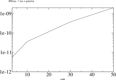
Figure 1: Predictions for LFV tau decay rates for degenerate heavy neutrinos as a function of $\tan\beta$. The remaining SUSY parameters are as for SPS4. The seesaw parameters are $m_{N}=10^{14}$ GeV and $R$ is any real orthogonal matrix. Here we have set $\theta_{13}=0^{\circ}$

3 Results for hierachical heavy neutrinos

We next present the results for the alternative case of hierarchical heavy neutrinos where we find rates that are, for some regions of the SUSY-seesaw parameter space, within the present and/or future experimental reach. In this case, the BRs are mostly sensitive to the heaviest mass $m_{N_{3}}$, $\tan\beta$, $\theta_{1}$ and $\theta_{2}$. The other input seesaw parameters $m_{N_{1}}$, $m_{N_{2}}$ and $\theta_{3}$ play a secondary role since the BRs do not strongly depend on them. The dependence on $m_{N_{1}}$ and $\theta_{3}$ appears only indirectly, once the requirement of a successfull BAU is imposed. We will comment more on this later.

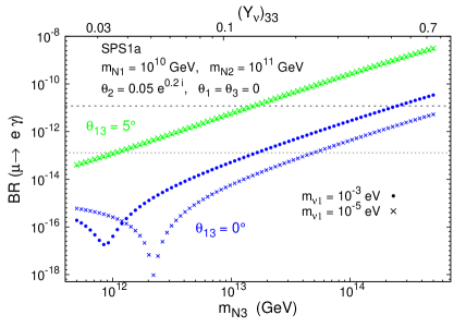
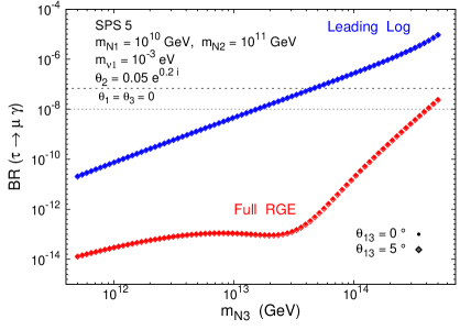
Figure 2: On the left, BR($\mu\to e\,\gamma$) as a function of $m_{N_{3}}$ for SPS 1a, with $m_{\nu_{1}}\,=\,10^{-5}$ eV and $m_{\nu_{1}}\,=\,10^{-3}$ eV (times, dots, respectively), and $\theta_{13}=0^{\circ},\,5^{\circ}$ (blue/darker, green/lighter lines). Baryogenesis is enabled by the choice $\theta_{2}\,=0.05\,e^{0.2\,i}$ ($\theta_{1}=\theta_{3}=0$). On the upper horizontal axis we display the associated value of $(Y_{\nu})_{33}$. On the right, BR($\tau\to\mu\,\gamma$) as a function of $m_{N_{3}}$ for SPS5, with $m_{\nu_{1}}\,=\,10^{-3}$ eV and $\theta_{2}\,=0.05\,e^{0.2\,i}$ ($\theta_{1}=\theta_{3}=0^{\circ}$). In both cases a dashed (dotted) horizontal line denotes the present experimental bound (future sensitivity).

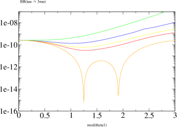
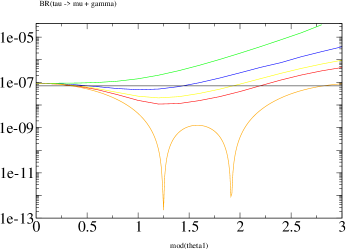
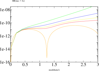
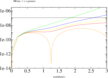
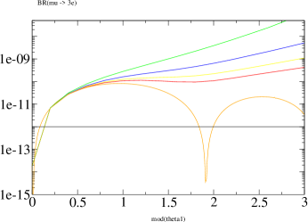
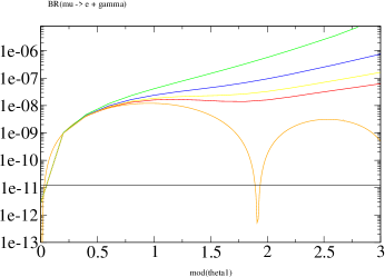
Figure 3: Predictions of LFV $\tau$ and $\mu$ decay rates as a function of $|\theta_{1}|$ for hierarchical heavy neutrinos, complex $R$-matrix, and for SPS4. The seesaw parameters are $\arg(\theta_{1})=0,\pi/10,\pi/8,\pi/6,\pi/4$ (lower to upper lines), $\theta_{2}=\theta_{2}=0$ and the heavy neutrino masses are $(m_{N_{1}},m_{N_{2}},m_{N_{3}})=(10^{8},2\times 10^{8},10^{14})$ GeV. The horizontal lines denote the present experimental bounds. Here we have set $\theta_{13}=0^{\circ}$

.

We display in Fig. 2 the predictions for BR$(\mu\to e\gamma)$ and BR$(\tau\to\mu\gamma)$ as a function of $m_{N_{3}}$, for a specific choice of the other input parameters. This figure clearly shows the strong sensitivity of the BRs to $m_{N_{3}}$. In fact, the BRs vary by as much as six orders of magnitude in the explored range of $5\times 10^{11}\,{\rm GeV}\leq m_{N_{3}}\leq 5\times 10^{14}\,{\rm GeV}$. Notice also that for the largest values of $m_{N_{3}}$ considered, the predicted rates for $\mu\to e\gamma$ are within the present experimental reach while those of $\tau\to\mu\gamma$ are only within the future experimental sensitivity. It is also worth mentioning that by comparing our full results with the LLog predictions, we find that the LLog approximation dramaticaly fails in some cases. In particular, for the SPS5 point, the LLog predictions overestimate the BRs by about four orders of magnitude. For the other points SPS4, SPS1a,b and SPS2 the LLog estimate is very similar to the full result, whereas for SPS3 it underestimates the full computation by a factor of three. In general, the divergence of the LLog and the full computation occurs for low $M_{0}$ and large $M_{1/2}$ [22, 23] and/or large $A_{0}$ values [2]. The failure of the LLog is more dramatic for SUSY scenarios with large $A_{0}$. Fig. 2 also shows that while in some cases (for instance SPS1a) the behaviour of the BR with $m_{N_{3}}$ does follow the expected LLog approximation (BR $\sim(m_{N_{3}}\log m_{N_{3}})^{2}$), there are other scenarios where this is not the case. A good example of this is SPS5. It is also worth commenting on the deep minima of BR$(\mu\to e\gamma)$ appearing in Fig. 2 for the lines associated with $\theta_{13}=0^{\circ}$. These minima are induced by the effect of the running of $\theta_{13}$, shifting it from zero to a negative value (or equivantly $\theta_{13}>0$ and $\delta=\pi$). In the LLog approximation, they can be understood as a cancellation occurring in the relevant matrix element of $Y_{\nu}^{\dagger}LY_{\nu}$, with $L_{ij}=\log(M_{X}/m_{N_{i}})\delta_{ij}$. Explicitly, the cancellation occurs between the terms proportional to $m_{N_{3}}\,L_{33}$ and $m_{N_{2}}\,L_{22}$ in the limit $\theta_{13}(m_{R})\to 0^{-}$ (with $\theta_{1}=\theta_{3}=0$). The depth of these minima is larger for smaller $m_{\nu_{1}}$, as is visible in Fig. 2.

Regarding the $\tan\beta$ dependence of the BRs we obtain that, similar to what was found for the degenerate case, the BR grow as $\tan^{2}\beta$. The hierarchy of the BR predictions for the several SPS points is dictated by the corresponding $\tan\beta$ value, with a secondary role being played by the given SUSY spectra. We again find the following generic hierarchy: BR_SPS4 $>$ BR_SPS1b $\gtrsim$ BR_SPS1a $>$ BR_SPS3 $\gtrsim$ BR_SPS2 $>$ BR_SPS5.

In what concerns to the $\theta_{i}$ dependence of the BRs, we have found that they are mostly sensitive to $\theta_{1}$ and $\theta_{2}$. The BRs are nearly constant with $\theta_{3}$. The predictions for all the LFV channels as functions of $\theta_{1}$ are shown in Fig. 3. From this figure we first see that the BRs basically follow the pattern of the $Y_{\nu}$ couplings as functions of $\theta_{1}$, including the appearance of pronounced dips at particular $|\theta_{1}|$ values for the real $\theta_{1}$ case. Although not displayed here, the results for $Y_{\nu}$ show that the largest predicted entries are $Y_{\nu}^{33}$ and $Y_{\nu}^{32}$, reaching values up to ${\cal O}(1)$ for the explored $\theta_{1}$ range (see also the left panel of Fig. 2). The main conclusion from Fig. 3 is that the predictions for BR$(\mu\to e\gamma)$, BR$(\mu\to 3e)$, BR$(\tau\to\mu\gamma)$ and BR$(\tau\to e\gamma)$ are above their corresponding experimental bound for specific values of $\theta_{1}$. Particularly, the LFV muon decay rates are well above their present experimental bounds for most of the explored $\theta_{1}$ values. Notice also that for SPS4 the predicted BR$(\tau\to\mu\gamma)$ values are very close to the present experimental reach even at $\theta_{1}=0$ (that is, $R=1$). We have also explored the dependence on $\theta_{2}$ and found similar results (not shown here), with the appearance of pronounced dips at particular real values of $\theta_{2}$ with the BR$(\mu\to e\gamma)$, BR$(\mu\to 3e)$ and BR$(\tau\to\mu\gamma)$ predictions being above the experimental bounds for some $\theta_{2}$ values.

We next address the sensitivity of the LFV BRs to $\theta_{13}$. We first present the results for the case $R=1$ and then discuss how this sensitivity changes when moving from this case towards the more general case of a complex $R$, taking into account additional constraints from the requirement of a succesfull BAU.

For $R=1$, the predictions of the BRs as functions of $\theta_{13}$, valid within the experimentally allowed range of $\theta_{13}$, $0^{\circ}\leq\theta_{13}\lesssim 10^{\circ}$, are illustrated in Fig. 4. In this figure we also include the present and future experimental sensitivities for all channels. We clearly see that the BRs of $\mu\to e\gamma$, $\mu\to 3e$, $\tau\to e\gamma$ and $\tau\to 3e$ are extremely sensitive to $\theta_{13}$, with their predicted rates varying many orders of magnitude along the explored $\theta_{13}$ interval. In the case of $\mu\to e\gamma$ this strong sensitivity was previously pointed out in Ref. [24]. The other LFV channels, $\tau\to\mu\gamma$ and $\tau\to 3\mu$ (not displayed here), are nearly insensitive to this parameter. The most important conclusion from Fig. 4 is that, for this choice of parameters, the predicted BRs for both muon decay channels, $\mu\to e\gamma$ and $\mu\to 3e$, are clearly within the present experimental reach for several of the studied SPS points. The most stringent channel is manifestly $\mu\to e\gamma$ where the predited BRs for all the SPS points are clearly above the present experimental bound for $\theta_{13}\gtrsim 5^{\circ}$. With the expected improvement in the experimental sensitivity to this channel, this would happen for $\theta_{13}\gtrsim 1^{\circ}$.

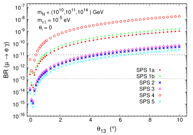
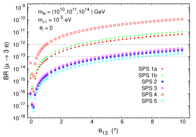
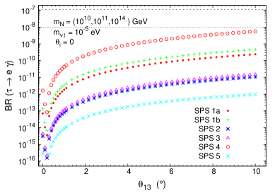
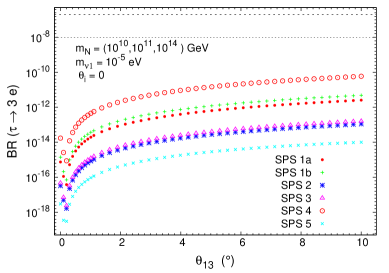
Figure 4: BR($\mu\to e\,\gamma$) and BR($\mu\to 3\,e$) as a function of $\theta_{13}$ (in degrees), for SPS 1a (dots), 1b (crosses), 2 (asterisks), 3 (triangles), 4 (circles) and 5 (times). A dashed (dotted) horizontal line denotes the present experimental bound (future sensitivity).

In addition to the generation of small neutrino masses, the seesaw mechanism offers the interesting possibility of baryogenesis via leptogenesis [25]. Thermal leptogenesis is an attractive and minimal mechanism to produce a successfull BAU which is compatible with present data, $n_{\mathrm{B}}/n_{\gamma}\,\approx\,(6.10\,\pm\,0.21)\,\times\,10^{-10}$ [26]. In the SUSY version of the seesaw mechanism, it can be successfully implemented provided that the following conditions can be satisfied. Firstly, Big Bang Nucleosynthesis gravitino problems have to be avoided, which is possible, for instance, for sufficiently heavy gravitinos. Since we consider the gravitino mass as a free parameter, this condition can be easily achieved. In any case, further bounds on the reheat temperature $T_{\mathrm{RH}}$ still arise from decays of gravitinos into Lightest Supersymmetric Particles (LSPs). In the case of heavy gravitinos, and neutralino LSPs masses in the range 100-150 GeV (which is the case of the present work), one obtains $T_{\mathrm{RH}}\lesssim 2\times 10^{10}$ GeV. In the presence of these constraints on $T_{\mathrm{RH}}$, the favoured region by thermal leptogenesis corresponds to small (but non-vanishing) complex $R$-matrix angles $\theta_{i}$. For vanishing $U_{\text{MNS}}$ CP phases the constraints on $R$ are basically $|\theta_{2}|,|\theta_{3}|\lesssim 1\,\mbox{rad}$ (mod $\pi$). Thermal leptogenesis also constrains $m_{N_{1}}$ to be roughly in the range $[10^{9}\>\mbox{GeV},10\times T_{\mathrm{RH}}]$. In the present work, we require the BAU to be within the interval $[10^{-10},10^{-9}]$, which contains the WMAP range, and choose the value of $m_{N_{1}}=10^{10}$ GeV in some of our plots. Similar studies of the constraints from leptogenesis on LFV rates have been done in [27].

Concerning the EDMs, which are clearly non-vanishing in the presence of complex $\theta_{i}$, we have checked that all the predicted values for the electron, muon and tau EDMs are well below the experimental bounds. In the following we therefore focus on complex but small $\theta_{2}$ values, leading to favourable BAU, and study its effects on the sensitivity to $\theta_{13}$. Similar results are obtained for $\theta_{3}$, but for shortness are not shown here.

Fig. 5 shows the dependence of the most sensitive BR to $\theta_{13}$, BR$(\mu\to e\,\gamma)$, on $|\theta_{2}|$. We consider two particular values of $\theta_{13}$, $\theta_{13}=0^{\circ}\,,5^{\circ}$ and choose SPS 1a. Motivated from the thermal leptogenesis favoured $\theta_{2}$-regions [2], we take $0\,\lesssim\,|\theta_{2}|\,\lesssim\,\pi/4$, with $\arg\theta_{2}\,=\,\{\pi/8\,,\,\pi/4\,,\,3\pi/8\}$. We display the numerical results, considering $m_{\nu_{1}}\,=\,10^{-5}$ eV and $m_{\nu_{1}}\,=\,10^{-3}$ eV, while for the heavy neutrino masses we take $m_{N}\,=\,(10^{10},\,10^{11},\,10^{14})$ GeV.

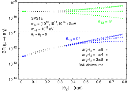
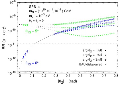
Figure 5: BR($\mu\to e\,\gamma$) as a function of $|\theta_{2}|$, for $\arg\theta_{2}\,=\,\{\pi/8\,,\,\pi/4\,,\,3\pi/8\}$ (dots, times, diamonds, respectively) and $\theta_{13}=0^{\circ}$, 5^∘ (blue/darker, green/lighter lines). We take $m_{\nu_{1}}\,=\,10^{-5}$ ($10^{-3}$) eV, on the left (right) panel. In all cases black dots represent points associated with a disfavoured BAU scenario and a dashed (dotted) horizontal line denotes the present experimental bound (future sensitivity).

There are several important conclusions to be drawn from Fig. 5. Let us first discuss the case $m_{\nu_{1}}\,=\,10^{-5}$ eV. We note that one can obtain a baryon asymmetry in the range $10^{-10}$ to $10^{-9}$ for a considerable region of the analysed $|\theta_{2}|$ range. Notice also that there is a clear separation between the predictions of $\theta_{13}=0^{\circ}$ and $\theta_{13}=5^{\circ}$, with the latter well above the present experimental bound. This would imply an experimental impact of $\theta_{13}$, in the sense that the BR predictions become potentially detectable for this non-vanishing $\theta_{13}$ value. With the planned MEG sensitivity [15], both cases would be within experimental reach. However, this statement is strongly dependent on the assumed parameters, in particular $m_{\nu_{1}}$. For instance, a larger value of $m_{\nu_{1}}=10^{-3}$ eV, illustrated on the right panel of Fig. 5, leads to a very distinct situation regarding the sensitivity to $\theta_{13}$. While for smaller values of $|\theta_{2}|$ the branching ratio displays a clear sensitivity to having $\theta_{13}$ equal or different from zero (a separation larger than two orders of magnitude for $|\theta_{2}|\lesssim 0.05$), the effect of $\theta_{13}$ is diluted for increasing values of $|\theta_{2}|$.

Let us now address the question of whether a joint measurement of the BRs and $\theta_{13}$ can shed some light on experimentally unreachable parameters, like $m_{N_{3}}$. The expected improvement in the experimental sensitivity to the LFV ratios supports the possibility that a BR could be measured in the future, thus providing the first experimental evidence for new physics, even before its discovery at the LHC. The prospects are especially encouraging regarding $\mu\to e\,\gamma$, where the experimental sensitivity will improve by at least two orders of magnitude. Moreover, and given the impressive effort on experimental neutrino physics, a measurement of $\theta_{13}$ will likely also occur in the future [28]. Given that, as previously emphasised, $\mu\to e\,\gamma$ is very sensitive to $\theta_{13}$, whereas this is not the case for BR($\tau\to\mu\,\gamma$), and that both BRs display the same approximate behaviour with $m_{N_{3}}$ and $\tan\beta$, we now propose to study the correlation between these two observables. This optimises the impact of a $\theta_{13}$ measurement, since it allows to minimise the uncertainty introduced from not knowing $\tan\beta$ and $m_{N_{3}}$, and at the same time offers a better illustration of the uncertainty associated with the $R$-matrix angles. In this case, the correlation of the BRs with respect to $m_{N_{3}}$ means that, for a fixed set of parameters, varying $m_{N_{3}}$ implies that the predicted point (BR($\tau\to\mu\,\gamma$), BR($\mu\to e\,\gamma$)) moves along a line with approximately constant slope in the BR($\tau\to\mu\,\gamma$)-BR($\mu\to e\,\gamma$) plane. On the other hand, varying $\theta_{13}$ leads to a displacement of the point along the vertical axis.

In Fig. 6, we illustrate this correlation for SPS 1a, choosing distinct values of the heaviest neutrino mass, and we scan over the BAU-enabling $R$-matrix angles (setting $\theta_{3}$ to zero) as

$$0\,\lesssim\,|\theta_{1}|\,\lesssim\,\pi/4\,,\quad-\pi/4\,\lesssim\,\arg\theta_{1}\,\lesssim\,\pi/4\,,$$

$$0\,\lesssim\,|\theta_{2}|\,\lesssim\,\pi/4\,,\quad\quad\,\,\,\,\,\,0\,\lesssim\,\arg\theta_{2}\,\lesssim\,\pi/4\,,$$

$$m_{N_{3}}\,=\,10^{12}\,,\,10^{13}\,,\,10^{14}\,\text{GeV}\,.$$ (1)

We consider the following values, $\theta_{13}=1^{\circ}$, $3^{\circ}$, $5^{\circ}$ and $10^{\circ}$, and only include in the plot the BR predictions which allow for a favourable BAU. Other SPS points have also been considered but they are not shown here for brevity (see [2]). We clearly observe in Fig. 6 that for a fixed value of $m_{N_{3}}$, and for a given value of $\theta_{13}$, the dispersion arising from a $\theta_{1}$ and $\theta_{2}$ variation produces a small area rather than a point in the BR($\tau\to\mu\,\gamma$)-BR($\mu\to e\,\gamma$) plane.

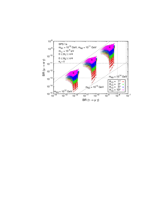
Figure 6: Correlation between BR($\mu\to e\,\gamma$) and BR($\tau\to\mu\,\gamma$) as a function of $m_{N_{3}}$, for SPS 1a. The areas displayed represent the scan over $\theta_{i}$ as given in Eq. (3). From bottom to top, the coloured regions correspond to $\theta_{13}=1^{\circ}$, $3^{\circ}$, $5^{\circ}$ and $10^{\circ}$ (red, green, blue and pink, respectively). Horizontal and vertical dashed (dotted) lines denote the experimental bounds (future sensitivities).

The dispersion along the BR($\tau\to\mu\,\gamma$) axis is of approximately one order of magnitude for all $\theta_{13}$. In contrast, the dispersion along the BR($\mu\to e\,\gamma$) axis increases with decreasing $\theta_{13}$, ranging from an order of magnitude for $\theta_{13}=10^{\circ}$, to over three orders of magnitude for the case of small $\theta_{13}$ ($1^{\circ}$). From Fig. 6 we can also infer that other choices of $m_{N_{3}}$ (for $\theta_{13}\in[1^{\circ},10^{\circ}]$) would lead to BR predictions which would roughly lie within the diagonal lines depicted in the plot. Comparing these predictions for the shaded areas along the expected diagonal “corridor”, with the allowed experimental region, allows to conclude about the impact of a $\theta_{13}$ measurement on the allowed/excluded $m_{N_{3}}$ values. The most important conclusion from Fig. 6 is that for SPS 1a, and for the parameter space defined in Eq. (3), an hypothetical $\theta_{13}$ measurement larger than $1^{\circ}$, together with the present experimental bound on the BR($\mu\to e\,\gamma$), will have the impact of excluding values of $m_{N_{3}}\gtrsim 10^{14}$ GeV. Moreover, with the planned MEG sensitivity, the same $\theta_{13}$ measurement can further constrain $m_{N_{3}}\lesssim 3\times 10^{12}$ GeV. The impact of any other $\theta_{13}$ measurement can be analogously extracted from Fig. 6.

As a final comment let us add that, remarkably, within a particular SUSY scenario and scanning over specific $\theta_{1}$ and $\theta_{2}$ BAU-enabling ranges for various values of $\theta_{13}$, the comparison of the theoretical predictions for BR($\mu\to e\,\gamma$) and BR($\tau\to\mu\,\gamma$) with the present experimental bounds allows to set $\theta_{13}$-dependent upper bounds on $m_{N_{3}}$. Together with the indirect lower bound arising from leptogenesis considerations, this clearly provides interesting hints on the value of the seesaw parameter $m_{N_{3}}$. With the planned future sensitivities, these bounds would further improve by approximately one order of magnitude. Ultimately, a joint measurement of the LFV branching ratios, $\theta_{13}$ and the sparticle spectrum would be a powerful tool for shedding some light on otherwise unreachable SUSY seesaw parameters. It is clear from this study that the connection between LFV and neutrino physics will play a relevant role for the searches of new physics.

References

- [1] E. Arganda and M. J. Herrero, Phys. Rev. D 73 (2006) 055003 [arXiv:hep-ph/0510405].
- [2] S. Antusch, E. Arganda, M. J. Herrero and A. Teixeira, arXiv:hep-ph/0607263, to appear in JHEP.
- [3] P. Minkowski, Phys. Lett. B 67 (1977) 421; M. Gell-Mann, P. Ramond and R. Slansky, in Complex Spinors and Unified Theories eds. P. Van. Nieuwenhuizen and D. Z. Freedman, Supergravity (North-Holland, Amsterdam, 1979), p.315 [Print-80-0576 (CERN)]; T. Yanagida, in Proceedings of the Workshop on the Unified Theory and the Baryon Number in the Universe, eds. O. Sawada and A. Sugamoto (KEK, Tsukuba, 1979), p.95; S. L. Glashow, in Quarks and Leptons, eds. M. Lévy et al. (Plenum Press, New York, 1980), p.687; R. N. Mohapatra and G. Senjanović, Phys. Rev. Lett. 44 (1980) 912.
- [4] Z. Maki, M. Nakagawa and S. Sakata, Prog. Theor. Phys. 28 (1962) 870; B. Pontecorvo, Sov. Phys. JETP 6 (1957) 429 [Zh. Eksp. Teor. Fiz. 33 (1957) 549]; Sov. Phys. JETP 7 (1958) 172 [Zh. Eksp. Teor. Fiz. 34 (1957) 247].
- [5] J. A. Casas and A. Ibarra, Nucl. Phys. B 618 (2001) 171 [arXiv:hep-ph/0103065].
- [6] F. Borzumati and A. Masiero, Phys. Rev. Lett. 57 (1986) 961.
- [7] B. C. Allanach et al., in Proc. of the APS/DPF/DPB Summer Study on the Future of Particle Physics (Snowmass 2001) ed. N. Graf, Eur. Phys. J. C 25 (2002) 113 [eConf C010630 (2001) P125] [arXiv:hep-ph/0202233].
- [8] J. Hisano, T. Moroi, K. Tobe and M. Yamaguchi, Phys. Rev. D 53 (1996) 2442 [arXiv:hep-ph/9510309].
- [9] W. Porod, Comput. Phys. Commun. 153 (2003) 275 [arXiv:hep-ph/0301101].
- [10] M. L. Brooks et al. [MEGA Collaboration], Phys. Rev. Lett. 83 (1999) 1521 [arXiv:hep-ex/9905013].
- [11] B. Aubert et al. [BABAR Collaboration], Phys. Rev. Lett. 96 (2006) 041801 [arXiv:hep-ex/0508012].
- [12] B. Aubert et al. [BABAR Collaboration], Phys. Rev. Lett. 95 (2005) 041802 [arXiv:hep-ex/0502032].
- [13] U. Bellgardt et al. [SINDRUM Collaboration], Nucl. Phys. B 299 (1988) 1.
- [14] B. Aubert et al. [BABAR Collaboration], Phys. Rev. Lett. 92 (2004) 121801 [arXiv:hep-ex/0312027].
-
[15]
S. Ritt [MEGA Collaboration], on the web page http://meg.web.psi.ch/docs/talks/
sritt/mar06novosibirsk/ritt.ppt. - [16] A. G. Akeroyd et al. [SuperKEKB Physics Working Group], arXiv:hep-ex/0406071.
- [17] T. Iijima, “Overview of Physics at Super B-Factory”, talk given at the 6th Workshop on a Higher Luminosity B Factory, KEK, Tsukuba, Japan, November 2004.
- [18] J. Aysto et al., arXiv:hep-ph/0109217.
-
[19]
The PRIME working group,
“Search for the Conversion Process at an Ultimate
Sensitivity of the Order of with PRISM”,
unpublished;
LOI to J-PARC 50-GeV PS, LOI-25,
http://psux1.kek.jp/jhf-np/LOIlist/
LOIlist.html - [20] Y. Kuno, Nucl. Phys. Proc. Suppl. 149 (2005) 376.
- [21] S. Pascoli, S. T. Petcov and C. E. Yaguna, Phys. Lett. B 564 (2003) 241 [arXiv:hep-ph/0301095].
- [22] S. T. Petcov, S. Profumo, Y. Takanishi and C. E. Yaguna, Nucl. Phys. B 676 (2004) 453 [arXiv:hep-ph/0306195].
- [23] P. H. Chankowski, J. R. Ellis, S. Pokorski, M. Raidal and K. Turzynski, Nucl. Phys. B 690 (2004) 279 [arXiv:hep-ph/0403180].
- [24] A. Masiero, S. K. Vempati and O. Vives, New J. Phys. 6 (2004) 202 [arXiv:hep-ph/0407325].
- [25] M. Fukugita and T. Yanagida, Phys. Lett. B 174 (1986) 45.
- [26] D. N. Spergel et al., arXiv:astro-ph/0603449.
- [27] S. T. Petcov, W. Rodejohann, T. Shindou and Y. Takanishi, Nucl. Phys. B 739 (2006) 208 [arXiv:hep-ph/0510404].
- [28] E. Ables et al. [MINOS Collaboration], Fermilab-proposal-0875; G. S. Tzanakos [MINOS Collaboration], AIP Conf. Proc. 721 (2004) 179; M. Komatsu, P. Migliozzi and F. Terranova, J. Phys. G 29 (2003) 443 [arXiv:hep-ph/0210043]; P. Migliozzi and F. Terranova, Phys. Lett. B 563 (2003) 73 [arXiv:hep-ph/0302274]; P. Huber, J. Kopp, M. Lindner, M. Rolinec and W. Winter, JHEP 0605 (2006) 072 [arXiv:hep-ph/0601266]; Y. Itow et al., arXiv:hep-ex/0106019; A. Blondel, A. Cervera-Villanueva, A. Donini, P. Huber, M. Mezzetto and P. Strolin, arXiv:hep-ph/0606111; P. Huber, M. Lindner, M. Rolinec and W. Winter, arXiv:hep-ph/0606119; J. Burguet-Castell, D. Casper, E. Couce, J. J. Gomez-Cadenas and P. Hernandez, Nucl. Phys. B 725 (2005) 306 [arXiv:hep-ph/0503021]; J. E. Campagne, M. Maltoni, M. Mezzetto and T. Schwetz, arXiv:hep-ph/0603172.