PITHA 06/09
hep-ph/0610322

Spectator scattering at NLO in non-leptonic
$B$ decays: Leading penguin amplitudes

M. Beneke and S. Jäger

Institut für Theoretische Physik E, RWTH Aachen
D–52056 Aachen, Germany

We complete the computation of the 1-loop ($\alpha_{s}^{2}$) corrections to hard spectator scattering in non-leptonic $B$ decays at leading power in $\Lambda/m_{b}$ by evaluating the penguin amplitudes. This extends the knowledge of these next-to-next-to-leading-order contributions in the QCD factorization formula for $B$ decays to a much wider class of final states, including all pseudoscalar-pseudoscalar, pseudoscalar-vector, and longitudinally polarized vector-vector final states, except final states with $\eta$ or $\eta^{\prime}$ mesons. The new 1-loop correction is significant for the colour-suppressed amplitudes, but turns out to be strongly suppressed for the leading QCD penguin amplitude $\alpha_{4}^{p}$. We provide numerical values of the phenomenological $P/T$ and $C/T$ amplitude ratios for the $\pi\pi$, $\pi\rho$ and $\rho\rho$ final states, and discuss corrections to several relations between electroweak penguin and tree amplitudes.

1 Introduction

In the QCD factorization framework [1, 2] the matrix elements of the effective weak interaction operators relevant to charmless non-leptonic $B$ decays $B\to M_{1}M_{2}$ take the (schematic) expression

$$\langle M_{1}M_{2}|Q_{i}|B\rangle=F^{BM_{1}}(0)\,\,T^{\mathrm{I}}_{i}*f_{M_{2}}\phi_{M_{2}}+T^{\mathrm{II}}_{i}*f_{B}\phi_{B+}*f_{M_{1}}\phi_{M_{1}}*f_{M_{2}}\phi_{M_{2}}$$ (1)

at leading order in the $1/m_{b}$ expansion, where $F^{BM_{1}}(0)$ denotes a $B\to M_{1}$ form factor at $q^{2}=0$, $f_{M}$ decay constants, and $\phi_{M}$ light-cone distribution amplitudes. The convolution kernels $T_{i}^{\rm I,II}$ are short-distance, and can be expanded in a perturbation series in the strong coupling $\alpha_{s}$. Precise calculations of these kernels are required to make the framework predictive. This is particularly the case for direct CP asymmetries, since at leading order in the $1/m_{b}$ expansion strong interaction phases arise only from these kernels, and only through loop diagrams.

The kernels $T_{i}^{\rm I}$ are currently known at order $\alpha_{s}$ [1, 2], which includes a 1-loop correction to “naive factorization”. The situation is different for $T_{i}^{\rm II}$, which always involves the exchange of a hard-collinear gluon with virtuality $m_{b}\Lambda$ ($\Lambda$ the strong interaction scale) with the spectator quark in the $B$ meson. Due to the presence of this additional scale it factorizes further according to [3]

$$T_{i}^{\rm II}=H^{\rm II}_{i}*J,$$ (2)

where the leading-order, ${\cal O}(\alpha_{s})$, term is associated with the tree approximation to both the hard kernels $H^{\rm II}_{i}$ and the hard-collinear kernel (“jet function”) $J$. In a previous paper [4] we computed the 1-loop corrections to the hard spectator-scattering kernel $H_{i}^{\rm II}$ for the (topological) “tree amplitudes” in two-body decays. Here we extend this computation to the case of the (topological) penguin amplitudes except for certain flavour-singlet terms that contribute only when $M_{2}$ is an $\eta$ or $\eta^{\prime}$ meson. Since $J$ is also known at one loop [5, 6], our result completes the set of spectator-scattering kernels at ${\cal O}(\alpha_{s}^{2})$.

The penguin amplitudes considered here provide the primary decay mechanism for $b\to s$ transitions. Their magnitudes and phases determine the size of the (direct) CP asymmetries in all charmless hadronic $B$ decays, since the necessary interference of decay amplitudes carrying different weak and strong phases always involves a penguin amplitude. In this respect it is worth noting that the strong phases are confined to $T_{i}^{\rm I}$ at order $\alpha_{s}$. At ${\cal O}(\alpha_{s}^{2})$ a new source of strong phases appears in the spectator-scattering kernels $T_{i}^{\rm II}$ via the one-loop correction to $H_{i}^{\rm II}$. In [4] we found for the case of the topological tree amplitudes that this contribution is comparable in size to its ${\cal O}(\alpha_{s})$ counterpart in $T_{i}^{\rm I}$. Consequently it can change qualitatively the picture of CP asymmetries, and may be important both in accounting for experimental data and in predictions for yet unobserved asymmetries, as well as for disentangling possible new physics contributions from the standard model background. In the case of penguin amplitudes similarly large contributions could occur. Spectator-scattering corrections to one of the four penguin amplitudes have already been calculated in [7]. We discuss the difference between that calculation and ours in Section 3.

The organization of the paper is as follows. In Section 2 we define the various flavour penguin amplitudes and discuss the diagram topologies that have to be calculated. We also set up the matching equations for the operators in the weak Hamiltonian to soft-collinear effective theory (SCET) that define the full set of hard-scattering kernels $H_{i}^{\rm II}$. These kernels are in turn expressed in terms of a complete set of “primitive” 1-loop hard-spectator-scattering kernels. Some details of their computation and the results for the primitive kernels are given in Section 3. In Sections 4 and 5 we obtain the numerical values of the corrections to the penguin amplitudes $\alpha_{i}(M_{1}M_{2})$, $\alpha_{i,\rm EW}(M_{1}M_{2})$ ($i=3,4$), and provide updated results for some phenomenologically important penguin-to-tree and electroweak penguin-to-tree amplitude ratios. We conclude in Section 6.

2 Structure of the penguin kernels

2.1 Flavour amplitudes

Our goal is to evaluate matrix elements of the the effective weak Hamiltonian for $b\to D$ transitions given by (see [2], where also numerical values of the Wilson coefficients $C_{i}$ are given)

$${\cal H}_{\mathrm{eff}} = \frac{G_{F}}{\sqrt{2}}\sum_{p=u,c}\,V_{pD}^{*}V_{pb}\left(C_{1}Q_{1}^{p}+C_{2}Q_{2}^{p}+\sum_{i=3\dots 10,7\gamma,8g}C_{i}Q_{i}\right)+\mathrm{h.c.},$$ (3)

$$Q_{1}^{p}=(\bar{p}_{a}b_{a})_{V-A}(\bar{D}_{b}u_{b})_{V-A},\qquad\quad Q_{2}^{p}=(\bar{p}_{b}b_{a})_{V-A}(\bar{D}_{a}u_{b})_{V-A},$$

$$Q_{3,5}=(\bar{D}_{a}b_{a})_{V-A}\sum_{q}(\bar{q}_{b}q_{b})_{V\mp A},$$

$$Q_{4,6}=(\bar{D}_{b}b_{a})_{V-A}\sum_{q}(\bar{q}_{a}q_{b})_{V\mp A},$$

$$Q_{7,9}=(\bar{D}_{a}b_{a})_{V-A}\sum_{q}\frac{3}{2}e_{q}(\bar{q}_{b}q_{b})_{V\pm A},$$

$$Q_{8,10}=(\bar{D}_{b}b_{a})_{V-A}\sum_{q}\frac{3}{2}e_{q}(\bar{q}_{a}q_{b})_{V\pm A},$$

$$Q_{7\gamma}=-\frac{em_{b}}{8\pi^{2}}\bar{D}\sigma_{\mu\nu}(1+\gamma_{5})F^{\mu\nu}b,\qquad Q_{8g}=-\frac{g_{s}m_{b}}{8\pi^{2}}\bar{D}\sigma_{\mu\nu}(1+\gamma_{5})G^{\mu\nu}b,$$

with $a,b$ denoting color, $D=d$ or $s$, and $(\bar{q}_{1}q_{2})_{V\mp A}=\bar{q}_{1}\gamma_{\mu}(1\mp\gamma_{5})q_{2}$. $e_{q}$ denotes the electric charge of quark $q$ in units of the positron charge $e$, and the sum over quarks extends over $q=u,d,s,c,b$. The definition of the dipole operators corresponds to the conventions $iD_{\mu}=i\partial_{\mu}+g_{s}G_{\mu}^{A}T^{A}+ee_{q}A_{\mu}$ and $\sigma_{\mu\nu}=\frac{i}{2}[\gamma_{\mu},\gamma_{\nu}]$. The effective Hamiltonian is understood to be renormalized in the NDR scheme as defined in [8].

To organize the flavour quantum numbers of the factorized matrix elements (1) we match ${\cal H}_{\mathrm{eff}}$ onto a transition operator ${\cal T}_{A}^{p}$ such that its matrix element is given by [9]

$$\langle M_{1}^{\prime}M_{2}^{\prime}|{\cal H}_{\rm eff}|\bar{B}\rangle=\sum_{p=u,c}\lambda_{p}^{(D)}\,\langle M_{1}^{\prime}M_{2}^{\prime}|{\cal T}_{A}^{p}|\bar{B}\rangle.$$ (4)

There are six different flavour structures required, resulting in

$${\cal T}_{A}^{p} = \delta_{pu}\,\alpha_{1}(M_{1}M_{2})\,A([\bar{q}_{s}u][\bar{u}D])+\delta_{pu}\,\alpha_{2}(M_{1}M_{2})\,A([\bar{q}_{s}D][\bar{u}u])$$ (5)

$$\mbox{}+\alpha_{3}^{p}(M_{1}M_{2})\,\sum_{q}A([\bar{q}_{s}D][\bar{q}q])+\alpha_{4}^{p}(M_{1}M_{2})\,\sum_{q}A([\bar{q}_{s}q][\bar{q}D])$$

$$\mbox{}+\alpha_{3,\rm EW}^{p}(M_{1}M_{2})\,\sum_{q}\frac{3}{2}\,e_{q}\,A([\bar{q}_{s}D][\bar{q}q])$$

$$\mbox{}+\alpha_{4,\rm EW}^{p}(M_{1}M_{2})\,\sum_{q}\frac{3}{2}\,e_{q}\,A([\bar{q}_{s}q][\bar{q}D]),\qquad$$

where the sums now extend only over $q=u,d,s$, and $\bar{q}_{s}$ denotes the spectator anti-quark in the $\bar{B}$ meson. The coefficients $\alpha_{i}^{p}(M_{1}M_{2})$ contain all dynamical information, while the arguments of $A$ encode the flavour composition of the final state and hence determine the final state to which a given term can contribute. The $\alpha_{i}$ parameters introduced in [9] are in close correspondence with the widely used “graphical” or “ topological” amplitudes [10]: $\alpha_{1}$ ($\alpha_{2}$) with the colour-allowed (colour-suppressed) tree amplitude; $\alpha_{4}^{p}$ with the QCD penguin amplitude; $\alpha^{p}_{3}$ with the QCD flavour-singlet penguin amplitude; and $\alpha^{p}_{3,\rm EW}$ ($\alpha^{p}_{4,\rm EW}$) with the colour-allowed (colour-suppressed) electroweak penguin amplitude. We define

$$\langle M_{1}^{\prime}M_{2}^{\prime}|\alpha_{i}^{p}(M_{1}M_{2})\,A([\ldots][\ldots])|\bar{B}_{q_{s}}\rangle\equiv\alpha_{i}^{p}(M_{1}^{\prime}M_{2}^{\prime})\,A_{M_{1}^{\prime}M_{2}^{\prime}}$$ (6)

whenever the quark flavours of the first and second square bracket match those of $M_{1}^{\prime}$ and $M_{2}^{\prime}$, respectively, and

$$\langle M_{1}^{\prime}M_{2}^{\prime}|\alpha_{i}^{p}(M_{1}M_{2})\,A([\ldots][\ldots])|\bar{B}_{q_{s}}\rangle\equiv\alpha_{i}^{p}(M_{2}^{\prime}M_{1}^{\prime})\,A_{M_{2}^{\prime}M_{1}^{\prime}}$$ (7)

whenever the quark flavours of the first and second square bracket match those of $M_{2}^{\prime}$ and $M_{1}^{\prime}$. The quantity $A_{M_{1}M_{2}}$ is given by

$$A_{M_{1}M_{2}} = i\frac{G_{F}}{\sqrt{2}}\left\{\begin{array}[]{lcl}m_{B}^{2}f_{+}^{BM_{1}}(0)f_{M_{2}}&&(M_{1},M_{2}=P)\\ -m_{B}m_{V_{1}}(n_{+}\cdot\epsilon^{*}_{M_{1}})A_{0}^{BM_{1}}(0)f_{M_{2}}&&(M_{1}=V,\,M_{2}=P)\\ -m_{B}m_{V_{2}}(n_{-}\cdot\epsilon^{*}_{M_{2}})f_{+}^{BM_{1}}(0)f_{M_{2}}&&(M_{1}=P,\,M_{2}=V)\\ m_{V_{1}}m_{V_{2}}(n_{+}\cdot\epsilon^{*}_{M_{1}})(n_{-}\cdot\epsilon^{*}_{M_{2}})A_{0}^{BM_{1}}(0)f_{M_{2}}&&(M_{1},M_{2}=V)\end{array}\right.$$ (12)

Here $f_{+}$ and $A_{0}$ denote pseudoscalar ($P$) and vector ($V$) meson form factors in the standard convention, and $f_{M_{2}}$ are the (longitudinal) decay constants. Here and in the remainder of the paper we consider only the longitudinal polarization state of the vector meson. This is sufficient for $B\to PV$ decays, but not for $B\to VV$, where two further transverse amplitudes are required for a complete description. The transverse amplitudes are, however, $1/m_{b}$-suppressed except for a certain electromagnetic amplitude [11]. (In (12) $m_{V_{1}}(n_{+}\cdot\epsilon^{*}_{M_{1}})$ is ${\cal O}(m_{B})$, hence all four expressions are of the same order in the heavy-quark expansion.)

In order to exemplify the notation consider the decay $\bar{B}_{d}\to\pi^{0}\rho^{0}$, for which $q_{s}=d$ and $D=d$. The spectator quark can go to either one of the two mesons, so $M_{1}$ can be $\pi^{0}$ or $\rho^{0}$. Hence, e.g.

$$\langle\pi^{0}\rho^{0}|\alpha_{4}^{p}(M_{1}M_{2})\sum_{q}A([\bar{d}q][\bar{q}d])|\bar{B}_{d}\rangle=\frac{1}{2}\left[\alpha_{4}^{p}(\pi^{0}\rho^{0})\,A_{\pi^{0}\rho^{0}}+\alpha_{4}^{p}(\rho^{0}\pi^{0})\,A_{\rho^{0}\pi^{0}}\right].$$ (13)

On the other hand,

$$\langle\pi^{0}\rho^{0}|\alpha_{3}^{p}(M_{1}M_{2})\sum_{q}A([\bar{d}d][\bar{q}q])|\bar{B}_{d}\rangle=0,$$ (14)

since $q=u,d$ contribute equally but with opposite sign for the mesons $\pi^{0}$ and $\rho^{0}$. We will assume isospin symmetry for the hadronic parameters of the mesons. It is then conventional to express the form factors and decays constants through one representative member of the isospin multiplet, for instance of the charged pion in the case of pions. With this convention (6) must be supplied with isospin Clebsch-Gordan coefficients $1,\pm 1/\sqrt{2}$ etc. from the flavour composition of the mesons. This is the origin of the factor $1/2$ in (13).

2.2 Diagram topologies

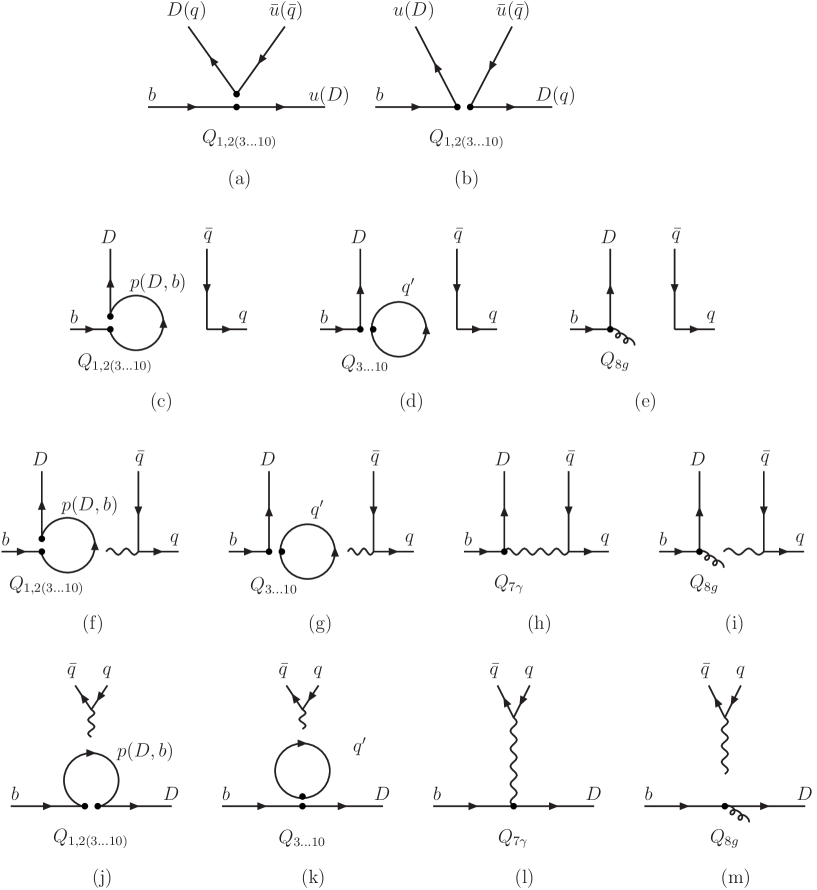
Figure 1: The various contractions of the external lines with the weak effective vertex, excluding arbitrarily many additional gluons. The connected fermion lines indicate the contraction of spinor indices. Terminology: (a) “right insertion”, (b) “wrong insertion”, (c) [(f)] “connected [photon] penguin”, (d) [(g)] “disconnected [photon] penguin”, (e) “magnetic insertion”. The photon can attach with its ‘loose’ end anywhere except on the line it originates from. There are several more topologies (h) through (m) contributing to electroweak penguin amplitudes (see text), and some topologies (not shown) only contributing when at least one final-state meson is an SU(3) flavour-singlet. For a more detailed explanation, see the text.

Let us denote, in Figure 1 and below, the initial and final state mesons by their flavour content. For instance, in Figure 1(a) the $\bar{B}$ meson has the flavour quantum numbers $[\bar{q}_{s}b]$, the final-state meson $M_{2}$ represented by the up-going quark lines has flavour content $[\bar{u}D]$, and the remaining meson $M_{1}$ $[\bar{q}_{s}u]$, where the $u$ line is drawn to the right. (The spectator line is not shown in the figure.)

The flavour amplitudes $\alpha_{i}^{p}$ in (5) receive perturbative contributions due to several ways of contracting the quark lines in the operators $Q_{i}$ with the valence quarks of the initial and final states, and possibly with each other. Considering first the case where $M_{2}$ does not have a flavour-singlet component, i.e. disregarding $\alpha_{3}^{p}$ for the moment, the contractions are shown in Figure 1. Here arbitrarily many gluons, that are not shown, may connect the quark lines, or originate from a quark line and connect with the spectator quark. We also consider photon exchange to lowest order, as indicated in Figure 1 (f) through (m). The last four contractions contribute only if a vector meson is involved, due to the intermediate photon.

Focusing for the moment on the operator $Q_{1}^{p}$, Figure 1(a), which we call the “right insertion”, gives the contribution to the colour-allowed tree amplitude $\alpha_{1}$ as can be seen by comparing the flavour labels of Figure 1(a) with (5). Contraction (b), the “wrong insertion”, gives the contribution to the colour-suppressed tree amplitude $\alpha_{2}$, while the “connected penguin” (c) contraction contributes to the (topological) penguin amplitude $\alpha_{4}^{p}$. For the operator $Q_{2}^{p}$, the roles of the “right” and “wrong” insertions are interchanged. The QCD penguin operators $Q_{3}\dots Q_{6}$ contribute, through all of the contractions (b) (with relabeling $u\to D$, $\bar{u}\to\bar{q}$, and $D\to q$) through (d), to the penguin amplitude $\alpha_{4}^{p}$ but not to $\alpha_{1,2}$. This is because of the sum over quarks already present in the effective weak interaction operator. The magnetic penguin operator $Q_{8g}$ contributes to $\alpha_{4}^{p}$ through contraction (e). In case of the electroweak penguin operators $Q_{7}\dots Q_{10}$ the right insertions (a) contribute to $\alpha_{3,\rm EW}^{p}$, and the wrong insertions to $\alpha_{4,\rm EW}^{p}$. However, insertions of $Q_{7}\dots Q_{10}$ into (c) and (d) do not contribute to the electroweak penguin amplitudes, but to electroweak corrections to the QCD penguin amplitudes, which we neglect. Thus, the second line of the figure corresponds to contributions to $\alpha_{4}^{p}$, while the first line can contribute to any of the $\alpha_{i}^{p}$ coefficients depending on the operator that is inserted.

The flavour-singlet QCD penguin amplitude $\alpha_{3}^{p}$ is more complicated [12]. There exists a contribution from the right insertion (a) which is similar to the ones discussed above, and which will be given below. In addition, however, there are penguin contractions, in which meson $M_{2}$ is made up only from gluons. The main reason for not calculating these contractions is that in case of the flavour-singlet penguin amplitude spectator scattering does not factorize in the form (1), but requires the introduction of a generalized non-local form factor [12]. Since the value of this form factor is unknown, the calculation of $\alpha_{3}^{p}$ is rather uncertain, and it is not useful to calculate loop corrections.

We also consider diagrams with photon exchange, but a complete calculation of QED corrections is beyond the scope of this paper. In fact, QED corrections to naive factorization have not even been considered for the simpler non-spectator contributions to the factorization formula up to now, except for an estimate of the soft photon contribution [15]. In general, electromagnetic corrections lead to isospin violation, incorporation of which requires an extension of the parameterization (5). Here, similar to [2, 9, 16] for the non-spectator contributions, we restrict ourselves to photon exchange diagrams that directly give the charge and flavour structure of $\alpha^{p}_{3,\rm EW}$ and $\alpha^{p}_{4,\rm EW}$. These “direct electroweak penguin” contributions are shown in the third and fourth line of Figure 1. When a photon is exchanged (besides, possibly, gluons) between the quark loop and the $\bar{q}q$ quark line, a contribution from $Q_{1}\ldots Q_{6}$ to the electroweak penguin amplitude $\alpha_{4,\rm EW}^{p}(M_{1}M_{2})$ arises for contractions (f) and (g), and to $\alpha_{3,\rm EW}^{p}(M_{1}M_{2})$ through contractions (j) and (k), if $M_{2}$ is a vector meson. Finally, the magnetic dipole operators $Q_{7\gamma}$, $Q_{8g}$ contribute to $\alpha_{4,\rm EW}^{p}$ (h,i) and, if $M_{2}=V$, to $\alpha_{3,\rm EW}^{p}$ via contractions (l) and (m). To make the distinction between “direct electroweak penguin” contributions and the remaining ones clearer we show in the first line of Figure 2 two diagrams that are included in our calculation of $\alpha^{p}_{4,\rm EW}$. On the other hand, the diagrams in the second line with the role of gluon and photon exchanged are not included, because they constitute isospin-violating contributions to the QCD penguin amplitude $\alpha^{p}_{4}$.

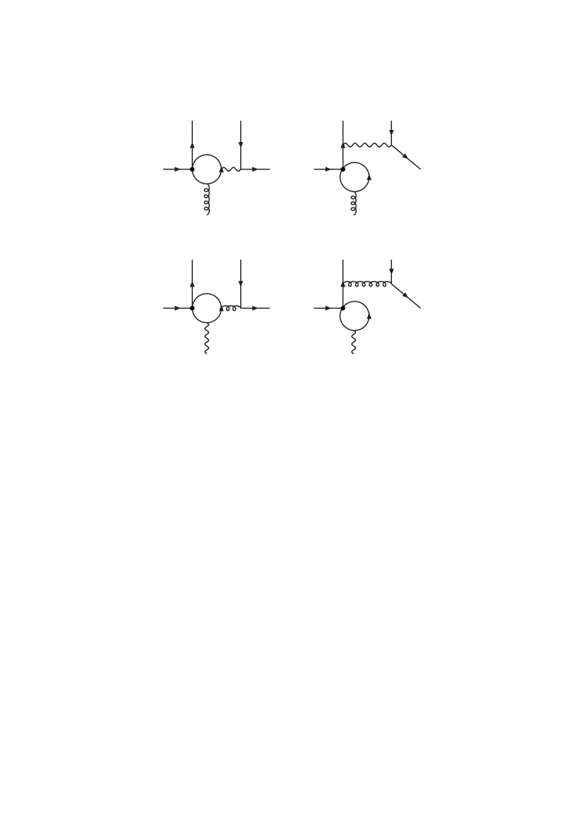
Figure 2: Examples of closely related diagrams that are interpreted as “direct electroweak penguin” contributions (first line), and as isospin-violating contributions (second line).

In summary, we see that there are a number of different short-distance coefficients, which in general receive contributions from several weak-interaction operators $Q_{i}$. The coefficients depend on (i) the Dirac structure of the operator $Q_{i}$, (ii) its colour structure, (iii) the type of contraction, (iv) for the penguin and magnetic contractions, whether a photon is exchanged or not, and (v) on the mass of the quark in the fermion loop.

2.3 Matching onto SCET_I

The hard-scattering kernels $T^{\rm I,II}_{i}$ can be determined by matching QCD$\to$SCET_I (resulting in $T_{i}^{\rm I}$, $H_{i}^{\rm II}$), and in the case of $T^{\rm II}$ subsequently SCET_I$\to$SCET_II  (resulting in $J$), whereby the kernels are identified with Wilson coefficients multiplying non-local operators in the effective theories [3, 4, 13, 17, 18, 19]. The two steps are equivalent to extracting, respectively, the hard and hard-collinear momentum regions from quark decay amplitudes according to the strategy of expanding Feynman diagrams by regions [20]. Single and double logarithms of ratios of scales are summed through renormalization group equations in SCET_I, and for the light-cone distribution amplitudes. Already in SCET_I modes corresponding to the two different light-like directions decouple at leading power in $\Lambda/m_{b}$, except for the contribution to the flavour-singlet QCD penguin amplitude $\alpha^{p}_{3}$ discussed in the previous subsection. Because of this, in SCET_I there are only right insertions, which moreover factor into matrix elements of two currents.

Following the notations and conventions of [13, 18], meson $M_{1}$, which picks up the spectator anti-quark from the $\bar{B}$ meson, moves in the direction of the light-like vector $n_{-}$. The collinear quark field for this direction is denoted by $\xi$ with $n\hskip-4.49997pt/_{-}\xi=0$, the corresponding collinear gluon field is $A_{c1}$. The second meson $M_{2}$ moves in the opposite direction $n_{+}$, and the collinear fields for this direction are $\chi$, satisfying $n\hskip-4.49997pt/_{+}\chi=0$, and $A_{c2}$. The heavy quark field $h_{v}$ is labeled by the time-like vector $v=(n_{-}+n_{+})/2$ with $v^{2}=1$, and $v\hskip-4.49997pt/h_{v}=h_{v}$.

In [4] we argued that, ignoring colour and flavour, to leading power in $1/m_{b}$ only two operators in SCET_I are needed to match the operators $Q_{1,2}^{p}$, as long as only current-current diagrams (contractions (a), (b) in Figure 1) are considered. The identification of these operators was based solely on power-counting arguments in SCET_I [18], except for the fact that only left-chiral $n_{+}$-collinear quark fields $\chi$ were considered due to the $(V-A)\times(V-A)$ structure of $Q_{1,2}^{p}$. Consequently, in addition to the extended flavour structures already discussed, the only novelty in the presence of the full set of operators $Q_{i}$ and diagram topologies is the appearance of a second leading operator in the collinear-2 sector, of opposite chirality, given by $(\bar{\chi}W_{c2})(tn_{-})n\hskip-4.49997pt/_{-}(1+\gamma_{5})(W_{c2}^{\dagger}\chi)(0)$. Mixed-chirality bilinears built from the $\chi$ fields necessarily involve either additional transverse derivatives or a Dirac matrix carrying an uncontracted transverse Lorentz index. In the former case they are power suppressed, while in the latter case the resultant operator cannot contribute to pseudoscalar or longitudinally polarized vector mesons. Once again, the flavour-singlet penguin amplitude $\alpha^{p}_{3}$ is special and requires operators with $n_{+}$-collinear gluons. Thus, excepting $\alpha^{p}_{3}$, the four SCET_I operators relevant to our calculation read

$$O_{L,R}^{\rm I}(t) = \Big{[}(\bar{\chi}W_{c2})(tn_{-}){\frac{{n\!\!\!/}_{-}}{2}}(1\mp\gamma_{5})(W_{c2}^{\dagger}\chi)\Big{]}\;\Big{[}\tilde{C}^{(A0)}_{f_{+}}\,({\bar{\xi}}W_{c1}){n\!\!\!/}_{+}(1-\gamma_{5})h_{v}$$

$$\hskip 28.45274pt-\frac{1}{m_{b}}\int d\hat{s}\,\tilde{C}^{(B1)}_{f_{+}}(\hat{s})\,(\bar{\xi}W_{c1}){n\!\!\!/}_{+}[W^{\dagger}_{c1}iD\hskip-5.89996pt/_{\perp c1}W_{c1}](sn_{+})(1+\gamma_{5})h_{v}\Big{]},$$

$$O^{\rm II}_{L,R}(t,s) = \frac{1}{m_{b}}\Big{[}(\bar{\chi}W_{c2})(tn_{-}){\frac{{n\!\!\!/}_{-}}{2}}(1\mp\gamma_{5})(W_{c2}^{\dagger}\chi)\Big{]}$$ (15)

$$\hskip 28.45274pt\times\Big{[}(\bar{\xi}W_{c1}){\frac{{n\!\!\!/}_{+}}{2}}[W^{\dagger}_{c1}iD\hskip-5.89996pt/_{\perp c1}W_{c1}](sn_{+})(1+\gamma_{5})h_{v}\Big{]},\quad$$

where $O_{L}^{\rm I}=O^{\rm I}$ and $O_{L}^{\rm II}=O^{\rm II}$ in [4]. The operators $O_{L,R}^{\rm I}$ include the short-distance coefficients $\tilde{C}^{(A0)}_{f_{+}}$, $\tilde{C}^{(B1)}_{f_{+}}(\hat{s})$ [6] such that their matrix elements are proportional to the form factor $f_{+}^{BM_{1}}(0)$ ($A_{0}^{BM_{1}}(0)$ for vector mesons) in QCD (not SCET_I). As usual, in (15) fields without position argument are at $x=0$, and the field products within the large brackets are colour-singlets. When including electromagnetic interactions the “direct electroweak penguins” contribute to the coefficient functions of $O^{\rm I,II}_{L,R}$, but there are also SCET_I operators of the above form with the transverse collinear gluon field $W^{\dagger}_{c1}iD\hskip-5.89996pt/_{\perp c1}W_{c1}$ replaced by a photon. This provides the sort of electromagnetic isospin-breaking, which as explained above we do not consider here. We can now take care of flavour by adding labels to the operators,

$$O^{\rm I,II}_{L,R}\to O^{\rm I,II}_{L,R}([\bar{q}_{s}q_{M_{1}}][\bar{q}_{M_{2}}q_{M_{2}}]),$$ (16)

where the labels $q_{M_{1,2}}$ and $\bar{q}_{M_{2}}$ give the flavours of the fields $\bar{\xi}$, $\bar{\chi}$, and $\chi$, respectively, and the redundant spectator label $\bar{q}_{s}$ has been added to match the notation (5). Then up the $n_{+}$-collinear gluon operators mentioned above, whose matrix elements contribute only to flavour-singlet $M_{2}$ (via a modification of $\alpha^{p}_{3}$), at leading power in $1/m_{b}$ the complete weak Hamiltonian (3) can be accounted for in SCET_I by

$${\cal H_{\rm eff}} = \frac{G_{F}}{\sqrt{2}}\sum_{p=u,c}V^{*}_{pD}V_{pb}\Bigg{(}\delta_{pu}\,\Bigg{\{}T_{1}^{\rm I}*O^{\rm I}_{L}([\bar{q}_{s}u][\bar{u}D])+H_{1}^{\rm II}*O^{\rm II}_{L}([\bar{q}_{s}u][\bar{u}D])$$

$$\qquad\quad\qquad\qquad+T_{2}^{\rm I}*O^{\rm I}_{L}([\bar{q}_{s}D][\bar{u}u])+H_{2}^{\rm II}*O^{\rm II}_{L}([\bar{q}_{s}D][\bar{u}u])\Bigg{\}}$$

$$\qquad+\sum_{k=L,R}\Bigg{\{}T_{3k}^{{\rm I},p}*\sum_{q}O^{\rm I}_{k}([\bar{q}_{s}D][\bar{q}q])+H_{3k}^{{\rm II},p}*\sum_{q}O^{\rm II}_{k}([\bar{q}_{s}D][\bar{q}q])$$

$$\qquad\qquad+T_{3k,\rm EW}^{{\rm I},p}*\sum_{q}\frac{3}{2}e_{q}O^{\rm I}_{k}([\bar{q}_{s}D][\bar{q}q])+H_{3k,\rm EW}^{{\rm II},p}*\sum_{q}\frac{3}{2}e_{q}O^{\rm II}_{k}([\bar{q}_{s}D][\bar{q}q])\Bigg{\}}\Bigg{)}$$

$$\qquad+\sum_{k=L,R}\Bigg{\{}T_{4k}^{{\rm I},p}*\sum_{q}O^{\rm I}_{k}([\bar{q}_{s}q][\bar{q}D])+H_{4k}^{{\rm II},p}*\sum_{q}O^{\rm II}_{k}([\bar{q}_{s}q][\bar{q}D])$$

$$\qquad\qquad+T_{4k,\rm EW}^{{\rm I},p}*\sum_{q}\frac{3}{2}e_{q}O^{\rm I}_{k}([\bar{q}_{s}q][\bar{q}D])+H_{4k,\rm EW}^{{\rm II},p}*\sum_{q}\frac{3}{2}e_{q}O^{\rm II}_{k}([\bar{q}_{s}q][\bar{q}D])\Bigg{\}}\Bigg{)}$$

where we employed the notation

$$T^{\rm I}_{ik}*O_{k}^{\rm I}=\int d\hat{t}\,\tilde{T}^{\rm I}_{ik}(\hat{t})O_{k}^{\rm I}(t),\qquad H_{ik}^{\rm II}*O_{k}^{\rm II}=\int d\hat{t}d\hat{s}\,\tilde{H}_{ik}^{\rm II}(\hat{t},\hat{s})O_{k}^{\rm II}(t,s)$$ (18)

with $\hat{s}=n_{+}p^{\prime}s=m_{B}s$, $\hat{t}=n_{-}q\,t=m_{B}t$, and $p^{\prime}$ ($q$) the momentum of $M_{1}$ ($M_{2}$). As in (5), the sums over $q$ extend only over the light quarks $u$, $d$, $s$, eventually implying that we neglect the “intrinsic charm” content of the mesons. Of the various matching coefficients in (2.3), the $T_{ik}^{\rm I}(u)=\int d\hat{t}\,e^{iu\hat{t}}\,\tilde{T}_{ik}^{\rm I}(\hat{t})$ are all known to the 1-loop order ($\alpha_{s}$) [1, 2, 9]. The 1-loop ($\alpha_{s}^{2}$) corrections to

$$H^{\rm II}_{1,2}(u,v)=\int d\hat{t}d\hat{s}\,e^{i(u\hat{t}+(1-v)\hat{s})}\,\tilde{H}^{\rm II}_{1,2}(\hat{t},\hat{s})$$ (19)

have been computed in [4]. In this paper we will compute the remaining coefficients $H^{{\rm II},p}_{4k}$, $H^{{\rm II},p}_{3k,\rm EW}$, $H^{{\rm II},p}_{4k,\rm EW}$, and parts of $H^{{\rm II},p}_{3k}$. We do not perform an expansion in $m_{c}/m_{b}$ in the matching calculation. The hard matching coefficients are therefore functions of the ratio $s_{c}=m_{c}^{2}/m_{b}^{2}$, whenever diagrams with internal charm-quark loops contribute.

The individual terms in (2.3) are in close correspondence with the $\alpha_{i}^{p}(M_{1}M_{2})$ amplitude parameters. The precise connection follows by evaluating the matrix element of (2.3). Because the SCET Lagrangian contains no leading-power interactions between the collinear-2 and collinear-1 fields, the matrix elements of $O^{\rm I}_{k}(t,s)$, $O^{\rm II}_{k}(t,s)$ fall apart into two factors each. For a pseudoscalar $M_{2}=P$,

$$\langle P|(\bar{\chi}W_{c2})(tn_{-}){\frac{{n\!\!\!/}_{-}}{2}}(1\pm\gamma_{5})(W_{c2}^{\dagger}\chi)|0\rangle=\mp\frac{if_{P}m_{B}}{2}\int_{0}^{1}du\,e^{iu\hat{t}}\,\phi_{P}(u),$$ (20)

while for a vector $M_{2}=V$ with polarization vector $\epsilon_{\mu}$ we have

$$\langle V|(\bar{\chi}W_{c2})(tn_{-}){\frac{{n\!\!\!/}_{-}}{2}}(1\pm\gamma_{5})(W_{c2}^{\dagger}\chi)|0\rangle=-\frac{if_{V}m_{V}}{2}\,n_{-}\cdot\epsilon^{*}\int_{0}^{1}du\,e^{iu\hat{t}}\,\phi_{V}(u),$$ (21)

such that only the longitudinal polarization state contributes. (The apparent suppression $m_{V}/m_{B}$ is cancelled by the polarization vector.) Here $\phi_{P}(u)$ ($\phi_{V}(u)$) denotes the leading-twist light-cone distribution amplitude of a pseudoscalar (longitudinally polarized vector) meson. Using [6]

$$\!\langle P|(\bar{\xi}W_{c1}){\frac{{n\!\!\!/}_{+}}{2}}[W^{\dagger}_{c1}iD\hskip-5.89996pt/_{\perp c}W_{c1}](sn_{+})(1+\gamma_{5})h_{v}|\bar{B}\rangle=-m_{b}m_{B}\int_{0}^{1}d\tau\,e^{i\tau\hat{s}}\,\Xi_{P}(\tau),$$ (22)

$$\!\langle V|(\bar{\xi}W_{c1}){\frac{{n\!\!\!/}_{+}}{2}}[W^{\dagger}_{c1}iD\hskip-5.89996pt/_{\perp c}W_{c1}](sn_{+})(1+\gamma_{5})h_{v}|\bar{B}\rangle=m_{b}m_{V}(n_{+}\cdot\epsilon^{*})\!\int_{0}^{1}d\tau\,e^{i\tau\hat{s}}\,\frac{m_{B}}{2m_{V}}\Xi_{\parallel}(\tau),$$

and defining

$$\hat{\Xi}_{M_{1}}(\tau)=\left\{\begin{array}[]{lll}\Xi_{P}(\tau)&&M_{1}=P\\[5.69046pt] \displaystyle\frac{m_{B}}{2m_{V}}\Xi_{\parallel}(\tau)&&M_{1}=V\end{array}\right.$$ (23)

we obtain

$$\alpha_{ik}^{p}(M_{1}M_{2}) = \int_{0}^{1}du\,T_{ik}^{\rm I}(u)\phi_{M_{2}}(u)$$ (24)

$$-\,\frac{1}{2F^{BM_{1}}(0)}\int_{0}^{1}dudv\,H_{ik}^{{\rm II},p}(u,v)\,\hat{\Xi}_{M_{1}}(1-v)\phi_{M_{2}}(u)$$

with $F^{BM_{1}}(0)=f_{+}^{BM_{1}}(0)$ when $M_{1}=P$, and $F^{BM_{1}}(0)=A_{0}^{BM_{1}}(0)$ for $M_{1}=V$. The index $i$ applies to $i=1,2,3,4,3\mbox{EW},4\mbox{EW}$, and $k=L,R$ except for $i=1,2$, where $k$ is empty (as is $p$). The two coefficients $\alpha_{1}(M_{1}M_{2})$, $\alpha_{2}(M_{1}M_{2})$ correspond to the “tree” flavour-amplitudes in (5), while the four “penguin” amplitudes are given by

$$\alpha^{p}_{3}(M_{1}M_{2}) = \alpha_{3L}^{p}(M_{1}M_{2})\mp\alpha_{3R}^{p}(M_{1}M_{2}),$$

$$\alpha^{p}_{4}(M_{1}M_{2}) = \alpha_{4L}^{p}(M_{1}M_{2})\mp\alpha_{4R}^{p}(M_{1}M_{2}),$$

$$\alpha^{p}_{3,\rm EW}(M_{1}M_{2}) = \alpha_{3L,\rm EW}^{p}(M_{1}M_{2})\mp\alpha_{3R,\rm EW}^{p}(M_{1}M_{2}),$$

$$\alpha^{p}_{4,\rm EW}(M_{1}M_{2}) = \alpha_{4L,\rm EW}^{p}(M_{1}M_{2})\mp\alpha_{4R,\rm EW}^{p}(M_{1}M_{2}).$$ (25)

Here the upper (lower) signs correspond to the case $M_{2}=P(V)$. The generalized form factors $\hat{\Xi}(\tau)$ factorize into light-cone distribution amplitudes after matching them to SCET_II [18]. The result is [6]

$$\hat{\Xi}(\tau)=\frac{m_{B}}{4m_{b}}\int_{0}^{\infty}\frac{d\omega}{\omega}\,\hat{f}_{B}\phi_{B+}(\omega)\int_{0}^{1}dw\,f_{M_{1}}\phi_{M_{1}}(w)\,J(\tau;w,\omega)$$ (26)

with $J=J_{\parallel}$, the hard-collinear kernel, known to order $\alpha_{s}^{2}$ [5, 6], and $\hat{f}_{B}$ the static $B$ meson decay constant as defined in [6].

2.4 Primitive kernels

Structure	Contraction
	(a)	(b)	(c)	(d)	(e)
$P_{LL}$	$r_{2},r_{1}$	$r_{1},r_{2}$	$s_{3},s_{4}$	$s_{1},s_{2}$	—
$P_{LR}$	$r_{4},r_{3}$	$\star$	$s_{3}^{\prime},s_{4}^{\prime}$	$s_{1}^{\prime},s_{2}^{\prime}$	—
$P_{\rm mag}$	—	—	—	—	$m_{1}$
	(f)	(g)	(h)	(i)
$P_{LL}$	$s_{3,\rm EW},s_{4,\rm EW}$	$s_{1,\rm EW},s_{2,\rm EW}$	—	—
$P_{LR}$	$s_{3,\rm EW}^{\prime},s_{4,\rm EW}^{\prime}$	$s_{1,\rm EW}^{\prime},s_{2,\rm EW}^{\prime}$	—	—
$P_{\rm mag}$	—	—	$m_{1,\rm EW}$	$m_{2,\rm EW}$
	(j)	(k)	(l)	(m)
$P_{LL}$	$s_{5,\rm EW},[s_{6,\rm EW}]$	$[s_{7,\rm EW}],s_{8,\rm EW}$	—	—
$P_{LR}$	$s_{5,\rm EW}^{\prime},s_{6,\rm EW}^{\prime}$	$[s_{7,\rm EW}^{\prime}],s_{8,\rm EW}^{\prime}$	—	—
$P_{\rm mag}$	—	—	$m_{3,\rm EW}$	$m_{4,\rm EW}$

Table 1: Definition of the primitive kernels. Where two kernels are given, the first corresponds to the colour structure of $Q_{1}$, the second to that of $Q_{2}$. The “star” means that there are no corresponding kernels at leading power. Kernels in parentheses vanish at the 1-loop order.

As explained at the end of Section 2.1, the short-distance coefficients encountered in matching an operator $Q_{i}$ in (3) can only depend on the Dirac structure, the colour structure, the type of contraction, the mass of the quark in penguin loops as far as present, and in the case of penguin contractions and of $Q_{8g}$, whether a photon is exchanged with the quark line on the right or not. Stripping the operators of all light-flavour and colour labels and an overall normalization factor, we encounter the full-QCD Dirac structures

$$P_{LL} = [\bar{q}\gamma^{\mu}(1-\gamma_{5})q][\bar{q}\gamma_{\mu}(1-\gamma_{5})b],$$

$$P_{RL} = [\bar{q}\gamma^{\mu}(1+\gamma_{5})q][\bar{q}\gamma_{\mu}(1-\gamma_{5})b],$$

$$P_{\rm mag} = -\frac{gm_{b}}{8\pi^{2}}\,\bar{q}\sigma_{\mu\nu}(1+\gamma_{5})b,$$ (27)

where $q$ denotes some light quark field (no summation implied) and $g=e$ or $g_{s}$. Their insertions into the contractions in Figure 1 define primitive kernels according to Table 1.

Of all these kernels, $r_{1}$ and $r_{2}$ have been given in [4]. The fact that these are sufficient to account for both “right” and “wrong” insertions (a) and (b) can be traced to Fierz symmetry. This is only valid because of the Fierz properties of the scheme used to define the renormalized effective weak Hamiltonian. In the case of penguin contractions, we will find, for instance, $s_{3}\neq s_{2}$, although the differences between such naively Fierz related kernels always assume a very simple form. In the present paper we also calculate the insertion (a) of the $P_{RL}$ structure. Insertion (b) results in a $1/m_{b}$ correction (related to the infamous power-suppressed but “chirally enhanced” scalar penguin amplitudes), so only two primitive kernels $r_{3,4}$ are needed. On the other hand, the fact that the penguin contractions (c) and (d) contribute for both $V-A\times V-A$ and $V-A\times V+A$ operators and for both colour structures requires the introduction of eight kernels $s_{i},s_{i}^{\prime}$, $i=1\ldots 4$. The remaining kernels are related to electroweak penguin terms and the insertions of the magnetic dipole operators.

We can now express the hard-scattering kernels $H_{ik}^{\rm II}$ in (2.3) in terms of these primitive building blocks as ($\bar{n}_{f}=n_{f}-2=3$ the number of flavours treated as massless)

$$H_{4L}^{{\rm II},p} = \frac{2}{N_{c}}\biggl{\{}\Bigl{[}\frac{1}{\bar{u}}+\frac{\alpha_{s}}{4\pi}r_{1}\Bigr{]}C_{3}+\frac{\alpha_{s}}{4\pi}r_{2}C_{4}$$ (28)

$$+\frac{\alpha_{s}}{4\pi}\Bigl{[}C_{1}s_{3}(s_{p})+C_{2}s_{4}(s_{p})+C_{3}\Big{(}s_{3}(0)+s_{3}(1)\Big{)}+C_{4}\Big{(}s_{4}(0)+s_{4}(1)\Big{)}$$

$$\qquad+\,C_{5}s_{3}^{\prime}(1)+C_{6}s_{4}^{\prime}(1)$$

$$\qquad+\Big{(}s_{1}(1)+s_{1}(s_{c})+\bar{n}_{f}s_{1}(0)\Big{)}C_{3}+\Big{(}s_{1}^{\prime}(1)+s_{1}^{\prime}(s_{c})+\bar{n}_{f}s_{1}^{\prime}(0)\Big{)}C_{5}$$

$$\qquad+\Big{(}s_{2}(1)+s_{2}(s_{c})+\bar{n}_{f}s_{2}(0)\Big{)}C_{4}+\Big{(}s_{2}^{\prime}(1)+s_{2}^{\prime}(s_{c})+\bar{n}_{f}s_{2}^{\prime}(0)\Big{)}C_{6}\Bigr{]}$$

$$\qquad+\,m_{1}C_{8g}\biggr{\}},$$

$$H_{4R}^{{\rm II},p} = 0,$$ (29)

$$H_{3L}^{{\rm II},p} = \frac{2}{N_{c}}\biggl{\{}\Bigl{[}\frac{1}{\bar{u}}+\frac{\alpha_{s}}{4\pi}r_{1}\Bigr{]}C_{4}+\frac{\alpha_{s}}{4\pi}r_{2}C_{3}\biggr{\}},$$ (30)

$$H_{3R}^{{\rm II},p} = \frac{2}{N_{c}}\biggl{\{}\Bigl{[}-\frac{1}{u}+\frac{\alpha_{s}}{4\pi}r_{3}\Bigr{]}C_{6}+\frac{\alpha_{s}}{4\pi}r_{4}C_{5}\biggr{\}},$$ (31)

$$H_{4L,\rm EW}^{{\rm II},p} = \frac{2}{N_{c}}\biggl{\{}\Bigl{[}\frac{1}{\bar{u}}+\frac{\alpha_{s}}{4\pi}r_{1}\Bigr{]}C_{9}+\frac{\alpha_{s}}{4\pi}r_{2}C_{10}$$ (32)

$$+\frac{2}{3}\frac{\alpha_{\mathrm{em}}}{4\pi}\Bigl{[}e_{u}C_{1}s_{3,\rm EW}(s_{p})+e_{u}C_{2}s_{4,\rm EW}(s_{p})+e_{d}C_{3}\Big{(}s_{3,\rm EW}(0)+s_{3,\rm EW}(1)\Big{)}$$

$$\qquad+\,e_{d}C_{4}\Big{(}s_{4,\rm EW}(0)+s_{4,\rm EW}(1)\Big{)}+e_{d}C_{5}s_{3,\rm EW}^{\prime}(1)+e_{d}C_{6}s_{4,\rm EW}^{\prime}(1)$$

$$\qquad+\Big{(}e_{d}s_{1,\rm EW}(1)+e_{u}s_{1,\rm EW}(s_{c})\Big{)}C_{3}+\Big{(}e_{d}s_{2,\rm EW}(1)+e_{u}s_{2,\rm EW}(s_{c})\Big{)}C_{4}$$

$$\qquad+\Big{(}e_{d}s_{1,\rm EW}^{\prime}(1)+e_{u}s_{1,\rm EW}^{\prime}(s_{c})\Big{)}C_{5}+\Big{(}e_{d}s_{2,\rm EW}^{\prime}(1)+e_{u}s_{2,\rm EW}^{\prime}(s_{c})\Big{)}C_{6}$$

$$\qquad+\,m_{1,\rm EW}C_{7\gamma}^{\rm eff}+m_{2,\rm EW}C_{8g}^{\rm eff}\Bigr{]}\biggr{\}},$$

$$H_{4R,\rm EW}^{{\rm II},p} = 0,$$ (33)

$$H_{3L,\rm EW}^{{\rm II},p} = \frac{2}{N_{c}}\biggl{\{}\Bigl{[}\frac{1}{\bar{u}}+\frac{\alpha_{s}}{4\pi}r_{1}\Bigr{]}C_{10}+\frac{\alpha_{s}}{4\pi}r_{2}C_{9}$$ (34)

$$+\frac{2}{3}\frac{\alpha_{\rm em}}{4\pi}\Bigl{[}e_{u}s_{5,\rm EW}(s_{p})C_{1}+e_{d}(s_{5,\rm EW}(0)+s_{5,\rm EW}(1))C_{3}$$

$$\qquad+\Big{(}e_{d}s_{8,\rm EW}(1)+e_{u}s_{8,\rm EW}(s_{c})\Big{)}C_{4}+\Big{(}e_{d}s_{8,\rm EW}^{\prime}(1)+e_{u}s_{8,\rm EW}^{\prime}(s_{c})\Big{)}C_{6}$$

$$\qquad+\,m_{3,\rm EW}C_{7\gamma}^{\rm eff}+m_{4,\rm EW}C_{8g}^{\rm eff}\Bigr{]}\biggr{\}},$$

$$H_{3R,\rm EW}^{{\rm II},p} = \frac{2}{N_{c}}\biggl{\{}\Bigl{[}-\frac{1}{u}+\frac{\alpha_{s}}{4\pi}r_{3}\Bigr{]}C_{8}+\frac{\alpha_{s}}{4\pi}r_{4}\,C_{7}$$ (35)

$$+\frac{2}{3}\frac{\alpha_{\rm em}}{4\pi}\Bigl{[}e_{u}s_{5,\rm EW}(s_{p})C_{1}+e_{d}(s_{5,\rm EW}(0)+s_{5,\rm EW}(1))C_{3}$$

$$\qquad+\Big{(}e_{d}s_{8,\rm EW}(1)+e_{u}s_{8,\rm EW}(s_{c})\Big{)}C_{4}+\Big{(}e_{d}s_{8,\rm EW}^{\prime}(1)+e_{u}s_{8,\rm EW}^{\prime}(s_{c})\Big{)}C_{6}$$

$$\qquad+\,m_{3,\rm EW}C_{7\gamma}^{\rm eff}+m_{4,\rm EW}C_{8g}^{\rm eff}\Bigr{]}\biggr{\}}.$$

Here the argument of the primitive kernels denotes the quark mass ratio $s_{q}=m_{q}^{2}/m_{b}^{2}$ with $q$ the quark flavour in the fermion loop of the penguin contraction. We also used $2e_{d}+e_{u}=0$ to simplify some of the electroweak penguin kernels, and introduced the standard “effective” Wilson coefficients, $C_{7\gamma}^{\rm eff}=C_{7\gamma}+e_{d}(C_{5}+N_{c}C_{6})$, $C_{8g}^{\rm eff}=C_{8g}+C_{5}$ to combine some ultraviolet contributions from fermion loops with the magnetic penguin coefficients. This convention modifies the primed primitive kernels such that $s_{5,\rm EW}^{\prime}$, $s_{6,\rm EW}^{\prime}$ vanish at one loop. For $H_{3L,\rm EW}^{{\rm II},p}$ and $H_{3R,\rm EW}^{{\rm II},p}$, the terms on the last three lines of each that stem from the insertions (j) to (l) in Figure 1 are identical, so they cancel out for $M_{2}=P$ as they should. To simplify the notation for $H_{3L,\rm EW}^{{\rm II},p}$ and $H_{3R,\rm EW}^{{\rm II},p}$, we already dropped the primitive kernels that vanish at one loop.

3 Computation and results

In this section we provide some technical remarks on the calculation and then summarize the results for the primitive kernels. We calculate the quark-gluon amplitude $b(p)\to q(q_{1})\bar{q}(q_{2})q(p^{\prime}_{1})g(p^{\prime}_{2})$ with insertions of $Q_{i}$ in QCD at 1-loop and subtract the corresponding SCET_I matrix elements to obtain the hard-scattering coefficient. Insertions of the magnetic dipole operators require only a tree-level calculation. At leading order in the $1/m_{b}$ expansion it is almost always possible to approximate the external momenta by their leading components $p=m_{b}v$, $q_{1}=um_{b}n_{+}/2$, $q_{2}=\bar{u}m_{b}n_{+}/2$, $p^{\prime}_{1}=vm_{b}n_{-}/2$, $p^{\prime}_{2}=\bar{v}m_{b}n_{-}/2$, which makes the calculation particularly simple in dimensional regularization. Exceptions to this are provided by diagrams with intermediate lines whose virtuality vanishes in this approximation, such as (a6), (e4) and all the diagrams in the third line of Figure 3.

3.1 Technical details

Vertex contractions (Figure 1 (a),(b))

The calculation of the new kernels $r_{3,4}$ related to insertions of $(V-A)\times(V+A)$ operators proceeds analogously to the one of $r_{1,2}$ described in detail in [4]. Only the right insertions need to be computed, since the wrong insertions match to power-suppressed SCET_I operators. Substituting $1-\gamma_{5}\to 1+\gamma_{5}$ in Eq. (17) of [4] to deal with the new $O^{\rm II}_{R}$ operators leads to a SCET operator basis, in which $O_{2-4}$ are no longer evanescent (vanishing in four dimensions). We can remedy this by choosing a new basis, in which all $\gamma^{\mu}_{\perp}$ stand to the right of all other transverse Dirac matrices. The treatment of IR singularities can then be done as in [4]. In the calculation of the matrix element of the evanescent operator $O_{2}$, one now encounters in addition to the contribution shown in Figure 4 of [4] a contribution related to the matrix element of the $\bar{\xi}A_{\perp c1}h_{v}$ part of the operator. This contribution can be deduced from the ultraviolet pole of $B$ in Eq. (39) of [6].

QCD penguin contractions (Figure 1 (c) – (e))

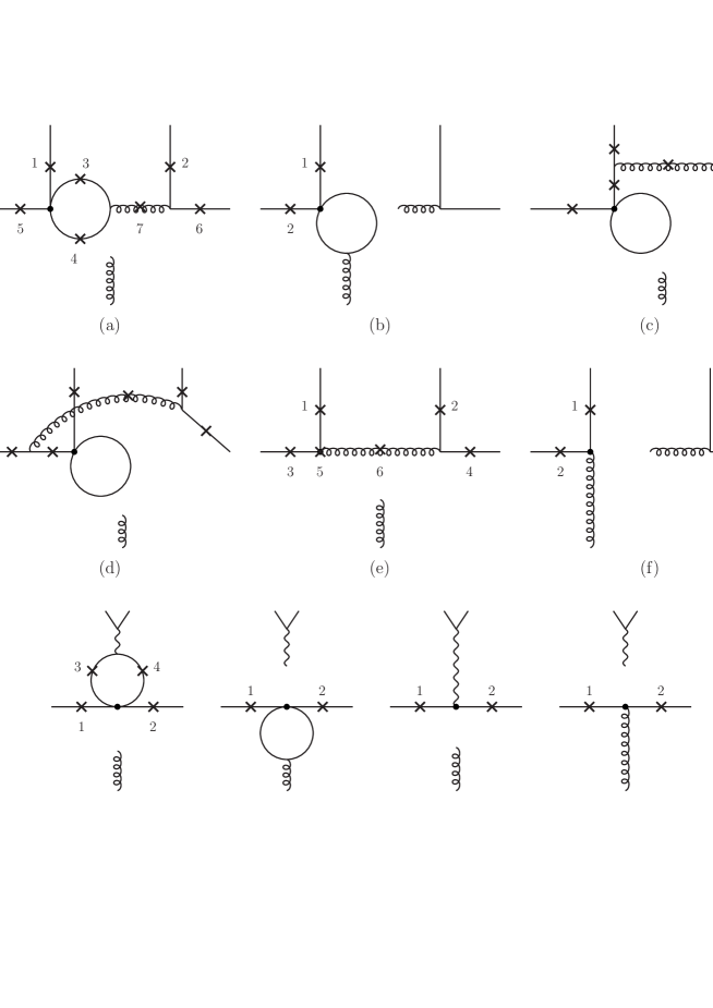
Figure 3: Summary of penguin-contraction diagrams. The ‘loose’ gluon or photon can attach to the crosses. Corresponding to diagram classes (a)-(f) there exist the diagrams with the horizontal gluon line replaced by a photon line. (For these (a7), (e5) and (e6) are absent.)

The penguin contraction diagrams are shown in Figure 3, of which the first two lines are relevant to the QCD penguin amplitude $\alpha^{p}_{4}$. The calculation of these diagrams is much simpler than the calculation of the vertex contractions. In particular, they are infrared finite, and no evanescent operators in SCET_I need to be considered. As in the case of the vertex contractions, one must take into account that the QCD factorization formula uses full-QCD form factors by convention, hence the second line in the definition of $Q^{I}_{L,R}$ in (15). As a consequence, the “form-factor subtraction”

$$2T^{\rm I(1)}_{ik}C^{(B1)(0)}_{f_{+}}=-2T^{\rm I(1)}_{ik}$$ (36)

(cf. Eq. (26) of [4]) has to be added to the diagrams in Figure 3 to obtain the final result for $H^{\rm II}_{ik}$, where $T^{\rm I(1)}_{ik}$ is the penguin contraction contribution to the 1-loop kernel $T^{I}_{ik}$. The form factor subtraction affects the structure of the result. For instance, we find that diagrams (e) and (f) in Figure 3 cancel exactly against the $C_{8g}$ term of the form factor subtraction, such that there is no dependence on $C_{8g}^{\rm eff}$ left, i.e. the primitive kernel $m_{1}=0$.

The “tadpole” contractions shown in Figure 3 (c) and (d) can be written as an effective flavour-changing two-point vertex

$$\frac{G_{F}}{\sqrt{2}}\left[\,\sum_{p=u,c}\,V_{pD}^{*}V_{pb}\right](C_{5}+N_{c}C_{6})\,A\,m_{b}^{3}\bar{D}(1+\gamma_{5})b,$$ (37)

where $A$ is a dimensionless, ultraviolet-divergent constant. However, the twelve tree diagrams with this vertex insertion vanish in their sum, so there is no contribution from this class of diagrams. We also find that the diagram classes (b) and (f) in Figure 3 actually vanish.

Penguin contractions to the hard-spectator scattering kernels relevant to the QCD penguin amplitude $\alpha^{p}_{4}$ have previously been calculated in [7]. In this paper the diagram classes (b), (c), (d) and (f) in Figure 3 are not considered (fortunately they all vanish), but diagrams (a5), (a6), (e3), (e4) and (e5) are also omitted, which is incorrect. The correct procedure includes these diagrams together with the form-factor subtraction discussed above. This seems to lead to significant numerical differences between our results and those of [7].

Electroweak penguin contractions (Figure 1 (f) – (m))

Electroweak penguin contributions from topologies specified in the first two lines in Figure 3 can be obtained by straightforward adjustment of colour factors from the corresponding QCD penguin diagrams.

The evaluation of the set of diagrams shown in the third line of the figure, which contributes to $\alpha^{p}_{3,\rm EW}$, requires some explanation, since the photon has small virtuality. When the vector meson $M_{2}$ is transverse, this leads to an enhancement [11], but for the longitudinal polarization state considered here the photon propagator cancels, and the diagrams contribute to the matching coefficients of SCET_I four-quark operators as shown for the non-spectator kernels $T^{\rm I}$ in [9].

We calculate this contribution by keeping the up-going quark and anti-quark on-shell ($q_{1}^{2}=q_{2}^{2}=0$), but we assign them a small transverse momentum $q_{2\perp}=-q_{1\perp}$, leading to a non-zero virtuality of the intermediate photon. Then a straightforward calculation shows that we may perform the substitution

$$\frac{-i}{q^{2}}\left(g^{\alpha\beta}-(1-\xi)\frac{q^{\alpha}q^{\beta}}{q^{2}}\right)\,\bar{q}(q_{1})\gamma_{\beta}q(q_{2})\to-2i\left(\frac{q^{\alpha}}{m_{b}q^{2}}-\frac{n_{-}^{\alpha}}{m_{b}^{2}}\right)\bar{\chi}{\frac{{n\!\!\!/}_{-}}{2}}\chi$$ (38)

in these diagrams. The $q^{\alpha}$ term contracts to zero with the remainder of the diagrams (after summing them all) as required by gauge invariance; in the second term the photon pole is manifestly cancelled. Nevertheless, one cannot set $q^{2}=0$ at this point, since the loop integrations result in $\ln q^{2}$. These infrared logarithms are subtracted by performing a SCET matching calculation. With $q^{2}\not=0$ the SCET matrix elements do not vanish and contain $\ln(q^{2}/\nu^{2})$. After matching the hard-scattering kernels are finite as $q^{2}\to 0$, but depend on the ultraviolet subtraction scale $\nu$, which is related to electromagnetic scale dependence of the longitudinal neutral vector meson decay constant. This scale dependence arises because (contrary to a widely held opinion) the electromagnetic current has an anomalous dimension in QED, which is precisely related to the penguin contractions as noted in [9]. See also [22] for an explanation of this point.

3.2 Results for the primitive kernels

The analytical results for the one-loop kernels are as follows.

Vertex contractions (Figure 1 (a),(b))

The kernels $r_{1}$ and $r_{2}$ can be found in [4]. The two new vertex kernels are related to these by

$$r_{3}(u,v) = -r_{1}(\bar{u},v)+(4\,C_{F}-C_{A})\Bigg{(}r_{2}(\bar{u},v)+\frac{3}{u}\Bigg{)},$$ (39)

$$r_{4}(u,v) = r_{2}(\bar{u},v)+\frac{6}{u}.$$ (40)

The colour factors are $C_{F}=(N_{c}^{2}-1)/(2N_{c})=4/3$ and $C_{A}=N_{c}=3$.

QCD penguin contractions (Figure 1 (c) – (e))

All kernels can be expressed in terms of the four functions $s_{1}$, $s_{3}^{F}$, $s_{3}^{A}$, $s_{4}^{\prime}$. With

$$s_{3}^{F}(s) = \frac{14}{9}\frac{1}{\bar{u}}-\frac{1}{\bar{u}v}-\frac{8(\bar{u}+uv)s}{3\bar{u}^{2}v}-\frac{2(1-2v)s}{\bar{u}v}C_{0}(s,\bar{u},v)$$ (41)

$$+\Bigg{(}\frac{8us}{3\bar{u}^{2}}-\frac{6-4u\bar{v}}{3\bar{u}\bar{v}}\Bigg{)}G_{0}(s,\bar{u})+\Bigg{(}\frac{4}{3}+\frac{8s}{3\bar{u}v}+\frac{2}{\bar{u}\bar{v}}\Bigg{)}G_{0}(s,\bar{u}v)$$

$$+\frac{2}{3\bar{u}}\bigg{(}\ln s+\ln\frac{m_{b}^{2}}{\mu^{2}}\bigg{)},$$

$$s_{3}^{A}(s) = -\frac{5}{18}\frac{1}{\bar{u}}+\frac{1}{3\bar{u}v}+\frac{2s}{\bar{u}^{2}v}+\frac{\bar{v}s}{\bar{u}v}C_{0}(s,\bar{u},v)$$ (42)

$$+\Bigg{(}\frac{1}{3\bar{u}\bar{v}}-\frac{2(3-v)s}{3\bar{u}^{2}v\bar{v}}\Bigg{)}G_{0}(s,\bar{u})+\Bigg{(}\frac{4s}{3\bar{u}^{2}\bar{v}}-\frac{1+2\bar{v}}{3\bar{u}\bar{v}}\Bigg{)}G_{0}(s,\bar{u}v)$$

$$-\frac{1}{3\bar{u}}\bigg{(}\ln s+\ln\frac{m_{b}^{2}}{\mu^{2}}\bigg{)},$$

we have

$$s_{1}(s) = \frac{1}{\bar{u}}-\frac{1}{2\,\bar{u}v}-\frac{(1-2v)s}{\bar{u}v}C_{0}(s,\bar{u},v)+\frac{1}{\bar{u}\bar{v}}(G_{0}(s,\bar{u}v)-G_{0}(s,\bar{u})),$$ (43)

$$s_{1}^{\prime}(s) = -s_{1}(s),$$ (44)

$$s_{2}(s) = s_{3}(s)-\Bigg{(}C_{F}-\frac{C_{A}}{2}\Bigg{)}\frac{2}{3\bar{u}},$$ (45)

$$s_{2}^{\prime}(s) = s_{3}(s)-(4C_{F}-C_{A})s_{1}(s)-\Bigg{(}C_{F}-\frac{C_{A}}{2}\Bigg{)}\frac{2}{3\bar{u}},$$ (46)

$$s_{3}(s) = C_{F}s_{3}^{F}(s)+C_{A}s_{3}^{A}(s),$$ (47)

$$s_{3}^{\prime}(1) = \Bigg{(}2C_{F}-\frac{C_{A}}{2}\Bigg{)}s_{4}^{\prime}(1),$$ (48)

$$s_{4}(s) = s_{1}(s),$$ (49)

$$s_{4}^{\prime}(1) = -\frac{2}{\bar{u}v}-\frac{2(2-\bar{u}\bar{v})}{\bar{u}v}C_{0}(1,\bar{u},v)-\frac{4}{\bar{u}\bar{v}}(G_{0}(1,\bar{u}v)-G_{0}(1,\bar{u})),$$ (50)

$$m_{1} = 0.$$ (51)

Here

$$G_{0}(s,x)=\frac{\sqrt{4s-x-i\epsilon}}{\sqrt{x}}\arctan\frac{\sqrt{x}}{\sqrt{4s-x-i\epsilon}},$$

$$C_{0}(s,x,y)=\frac{2}{x(1-y)}\Bigg{(}\arctan^{2}\sqrt{\frac{xy}{4s-xy-i\epsilon}}-\arctan^{2}\sqrt{\frac{x}{4s-x-i\epsilon}}\,\Bigg{)}.$$ (52)

Electroweak penguin contractions (Figure 1 (f) – (m))

$$s_{1,\rm EW}(s) = N_{c}\Bigg{(}s_{3}^{F}(s)-2s_{1}(s)-\frac{2}{3\bar{u}}\Bigg{)},$$ (53)

$$s^{\prime}_{1,\rm EW}(s) = s_{1,\rm EW}(s),$$ (54)

$$s_{2,\rm EW}(s) = s_{3}^{F}(s)-\frac{2}{3\bar{u}},$$ (55)

$$s^{\prime}_{2,\rm EW}(s) = s_{2,\rm EW}(s)-4s_{1}(s),$$ (56)

$$s_{3,\rm EW}(s) = s_{3}^{F}(s),$$ (57)

$$s^{\prime}_{3,\rm EW}(1) = 2s_{4}^{\prime}(1),$$ (58)

$$s_{4,\rm EW}(s) = N_{c}(s_{3}^{F}(s)-2s_{1}(s)),$$ (59)

$$s^{\prime}_{4,\rm EW}(1) = 0,$$ (60)

$$m_{1,\rm EW} = 0,$$ (61)

$$m_{2,\rm EW} = 0,$$ (62)

$$s_{5,\rm EW}(s) = \left\{\begin{array}[]{ll}N_{c}\bigg{(}6+2i\pi-2\ln\bar{v}-2\,{\displaystyle\ln\frac{m_{b}^{2}}{\nu^{2}}}\bigg{)}&\quad(s=0),\\[11.38092pt] N_{c}\Big{(}6-4G_{0}(s,\bar{v})+4sC_{0}(s,\bar{v},0)\Big{)}&\quad(s\not=0),\end{array}\right.$$ (65)

$$s_{8,\rm EW}(s) = s_{5,\rm EW}(s),$$ (66)

$$s^{\prime}_{8,\rm EW}(s) = -s_{5,\rm EW}(s),$$ (67)

$$m_{3,\rm EW} = 4N_{c},$$ (68)

$$m_{4,\rm EW} = 0.$$ (69)

The kernels $s_{6,\rm EW}$, $s_{7,\rm EW}$, $s^{\prime}_{7,\rm EW}$ vanish. The kernels $s^{\prime}_{5,\rm EW}$ and $s^{\prime}_{6,\rm EW}$ vanish after the rearrangement of Wilson coefficients discussed after (35). The scale $\nu$ in $s_{5,\rm EW}$ is due to the electromagnetic scale dependence of the neutral vector meson decay constant. In the following we no longer distinguish $\nu$ from the matching scale $\mu$ in the other expressions.

4 Numerical penguin amplitudes

In this section we study the numerical values of the calculated corrections to the penguin amplitudes $\alpha^{p}_{i}(M_{1}M_{2})$, $\alpha^{p}_{i,\rm EW}(M_{1}M_{2})$ ($i=3,4$), and provide updated results for some phenomenologically important penguin-to-tree and penguin-to-penguin amplitude ratios.

4.1 Input parameters

Parameter	Value/Range	Parameter	Value/Range
$\Lambda_{\overline{\mathrm{MS}}}^{(5)}$	0.225	$\mu_{b}$	$4.8^{+4.8}_{-2.4}$
$m_{c}$	$1.3\pm 0.2$	$\mu_{\mathrm{hc}}$	$1.5\pm 0.6$
$m_{s}$(2 GeV)	$0.09\pm 0.02$	$f_{B_{d}}$	$0.21\pm 0.02$
$(m_{u}+m_{d})/m_{s}$	0.0826	$f_{\pi}\,[f_{K}]$	0.131 [0.16]
$m_{b}$	4.8	$f^{B\pi}_{+}(0)$	$0.25\pm 0.05$
$\bar{m}_{b}(\bar{m}_{b})$	4.2	$f^{BK}_{+}(0)$	$0.34\pm 0.05$
$|V_{cb}|$	$0.0415\pm 0.0010$	$A_{0}^{B\rho}(0)$	$0.32\pm 0.05$
$|V_{ub}/V_{cb}|$	$0.09\pm 0.02$	$\lambda_{B}$(1 GeV)	$0.35\pm 0.15$
$\gamma$	$(70\pm 20)^{\circ}$	$\sigma_{1}$(1 GeV)	$1.5\pm 1$
$\tau(B^{-})$	1.64 ps	$\sigma_{2}$(1 GeV)	$3\pm 2$
$\tau(B_{d})$	1.53 ps	$a^{\bar{K}}_{1}$(2 GeV)	$0.06\pm 0.06$
		$a^{\pi,\bar{K}}_{2}$(2 GeV)	$0.2\pm 0.15$

Table 2: List of input parameters. Dimensionful parameters are given in units of 1 GeV.

The calculation of non-leptonic decay amplitudes needs several input parameters, which we summarize in Table 2. These are fundamental parameters such as the strong coupling, quark masses and CKM parameters; the matching and renormalization scale parameters $\mu_{b}$ and $\mu_{\rm hc}$ (see following subsection); and hadronic parameters related to decay constants, form factors and light-cone distribution amplitudes of the mesons.

There has been significant progress in the calculation of the first few Gegenbauer moments of the pion and kaon light-cone distribution amplitudes from QCD sum rules and lattice QCD [23, 24], which leads to a change in the corresponding entries in the table compared to earlier analyses. Less is known about the moments of the $B$ meson distribution amplitude,

$$\frac{1}{\lambda_{B}(\mu)}\equiv\int_{0}^{\infty}\frac{d\omega}{\omega}\,\phi_{B+}(\omega;\mu),\qquad\sigma_{n}(\mu)\equiv\lambda_{B}(\mu)\int_{0}^{\infty}\frac{d\omega}{\omega}\,\phi_{B+}(\omega;\mu)\,\ln^{n}\frac{\mu}{\omega}.$$ (70)

The logarithmic moments enter only in the 1-loop correction to the hard-collinear kernel $J$ in (26). However, $\lambda_{B}$ is very important, because the hard spectator-scattering contribution to the decay amplitudes is directly proportional to $1/\lambda_{B}$. The value of $\lambda_{B}$ adopted here follows [1] and represents a compromise between QCD sum rules and models of the B meson distribution amplitude that seem to favour larger values [25] and data that favour smaller values [4, 9]. Recent evaluations of the $B\to\pi$ form factor at $q^{2}=0$ also tend to smaller values [26], and we have therefore adjusted the input to the number taken in scenario S4 of [9]. The difference in $F^{B\pi}(0)$ vs. $F^{BK}(0)$ is consistent with the large SU(3) breaking found in [23, 26].

Parameters for mesons other than pions and kaons or parameters not given in the Table are taken from [9].

4.2 Renormalization group improvement and numerical implementation

Our main task is to evaluate the integrals

$$I=-\frac{1}{2F^{BM_{1}}(0)}\int_{0}^{1}dudv\,H_{ik}^{{\rm II},p}(u,v;\mu_{\rm hc})\,\hat{\Xi}_{M_{1}}(1-v;\mu_{\rm hc})\phi_{M_{2}}(u;\mu_{\rm hc})$$ (71)

in (24) with $\hat{\Xi}_{M_{1}}(1-v;\mu_{\rm hc})$ given in (26). Hard spectator scattering depends on the two scales $\mu_{b}\sim m_{b}$ and $\mu_{\rm hc}\sim\sqrt{m_{b}\Lambda}$. In the previous equation we indicated the renormalization scale in the arguments of all quantities. To avoid formally large logarithms of the ratio of the two scales we need $H_{ik}^{{\rm II},p}$ at $\mu_{\rm hc}$ in this equation. On the other hand, our calculation refers to matching the effective weak Hamiltonian to SCET_I at the scale $\mu_{b}$, i.e. the scale $\mu$ in Section 3.2 is $\mu_{b}$. In the following we explain the evolution of the hard-scattering coefficient to $\mu_{\rm hc}$, and the subsequent numerical evaluation of the integrals $I$.

The renormalization-group evolution of the hard-scattering coefficients is the same for all coefficients and can be written as

$$H_{ik}^{{\rm II},p}(u,v;\mu_{\rm hc}) = e^{-S(\mu_{b},\mu_{\rm hc})}\int_{0}^{1}du^{\prime}dv^{\prime}\,U_{\rm BL}(u,u^{\prime};\mu_{b},\mu_{\rm hc})$$ (72)

$$\times U_{\parallel}(1-v,1-v^{\prime};\mu_{b},\mu_{\rm hc})H_{ik}^{{\rm II},p}(u^{\prime},v^{\prime};\mu_{b}).$$

This follows because the evolution function factorizes into a term from the Brodsky-Lepage kernel [27] for the evolution of light-meson distribution amplitudes, and a Sudakov suppression factor times the evolution kernel for the so-called SCET B1-type currents [5, 6]. (The arguments of $U_{\parallel}$ follow the convention of [6], where they refer to the gluon momentum fraction in the B1-type operator, which is $1-v$.) The $U_{\rm BL}$ factor can be used to evolve $\phi_{M_{2}}(u;\mu_{\rm hc})$ to the scale $\mu_{b}$, so (71) reads

$$I = -\frac{1}{2F^{BM_{1}}(0)}\,e^{-S(\mu_{b},\mu_{\rm hc})}\int_{0}^{1}dudv^{\prime}\,\phi_{M_{2}}(u;\mu_{b})H_{ik}^{{\rm II},p}(u,v^{\prime};\mu_{b})$$ (73)

$$\times\int_{0}^{1}dv\,U_{\parallel}(1-v,1-v^{\prime};\mu_{b},\mu_{\rm hc})\,\hat{\Xi}_{M_{1}}(1-v;\mu_{\rm hc}).$$

The hard-scattering coefficients can be divided into two terms,

$$H_{ik}^{{\rm II},p}=H_{Vik}^{{\rm II},p}+H_{Pik}^{{\rm II},p},$$ (74)

referring to the vertex contractions (primitive kernels $r_{k}$) and penguin contractions (the others). The renormalization-group evolution and numerical evaluation of the first part is done exactly as described in Section 4.2 of [4]. In the following we discuss only the second part. This part begins at order $\alpha_{s}$ (or $\alpha_{\rm em}$), hence it is sufficient to evaluate $\hat{\Xi}_{M_{1}}$ in the tree approximation (order $\alpha_{s}$) for the hard-collinear kernel $J$ resulting in

$$\hat{\Xi}_{M_{1}}(1-v;\mu_{\rm hc})=-\frac{\pi C_{F}}{N_{c}}\frac{\alpha_{s}(\mu_{\rm hc})f_{M_{1}}\hat{f}_{B}(\mu_{\rm hc})}{m_{b}\lambda_{B}(\mu_{\rm hc})}\frac{\phi_{M_{1}}(v;\mu_{\rm hc})}{\bar{v}}.$$ (75)

Now we expand $\phi_{M_{1}}(v;\mu_{\rm hc})$ into Gegenbauer polynomials

$$\phi_{M_{1}}(v;\mu_{\rm hc})\,=\,6v\bar{v}\sum\limits_{n=0}^{\infty}a_{n}^{M_{1}}(\mu_{\rm hc})C^{(3/2)}_{n}(2v-1),$$ (76)

where $a_{n}^{M_{1}}(\mu_{\rm hc})$ are the Gegenbauer moments ($a_{0}^{M_{1}}(\mu_{\rm hc})=1$), and define

$${\cal C}_{n}(v;\mu_{b},\mu_{\rm hc})=\int_{0}^{1}dw\,6wC^{(3/2)}_{n}(2w-1)\,U_{\parallel}(1-w,1-v;\mu_{b},\mu_{\rm hc}).$$ (77)

Inserting this into (73) we obtain

$$I = \frac{f_{M_{1}}\hat{f}_{B}(\mu_{\rm hc})}{m_{b}F^{BM_{1}}(0)\lambda_{B}(\mu_{\rm hc})}\frac{\pi\alpha_{s}(\mu_{\rm hc})C_{F}}{2N_{c}}\,e^{-S(\mu_{b},\mu_{\rm hc})}$$ (78)

$$\times\sum\limits_{n=0}^{\infty}a_{n}^{M_{1}}(\mu_{\rm hc})\int_{0}^{1}dudv\,\phi_{M_{2}}(u;\mu_{b})\,H_{Pik}^{{\rm II},p}(u,v;\mu_{b})\,{\cal C}_{n}(v;\mu_{b},\mu_{\rm hc}).$$

It remains to calculate the ${\cal C}_{n}(v;\mu_{b},\mu_{\rm hc})$. This can be done by solving numerically the integro-differential equation

$$\mu\frac{d}{d\mu}\,{\cal C}_{n}(v;\mu,\mu_{\rm hc})=-\int_{0}^{1}dw\,\gamma_{\parallel}(1-v,1-w)\,{\cal C}_{n}(w;\mu,\mu_{\rm hc})$$ (79)

subject to the initial condition ${\cal C}_{n}(v;\mu_{\rm hc},\mu_{\rm hc})=6vC^{(3/2)}_{n}(2v-1)$, which follows from the defining equation (77) and the renormalization-group equation for $U_{\parallel}$. Here $\gamma_{\parallel}(\tau,\tau^{\prime})$ is the leading-order anomalous dimension of the B1-type currents [5, 6] (Eq. (99) in [6]). When this is done, the leading-logarithmic terms are summed to all orders, and (78) is free from formally large logarithms of the ratio of $m_{b}$ and $\sqrt{m_{b}\Lambda}$.

We truncate the Gegenbauer expansion of $\phi_{M_{1}}$ and $\phi_{M_{2}}$ after the second moment, so (78) is a sum of nine terms, each proportional to a product of two Gegenbauer moments. For fixed $\mu_{\rm hc}$ and $\mu_{b}$ the evolution equation and the remaining integrals can be solved numerically. In practice, we wish to construct a code that allows us to vary the scales freely in order to estimate theoretical errors. The numerical evaluation is then too time-consuming. We therefore proceed as follows. First we solve the evolution equation (79) by successive approximation up to the second order. Since the leading-order anomalous dimension $\gamma_{\parallel}$ depends on $\mu$ only through $\alpha_{s}(\mu)$, it is convenient to introduce a variable $x$ via

$$\mu\frac{d}{d\mu}=\beta(\alpha_{s})\frac{d}{d\alpha_{s}}=-\frac{\alpha_{s}(\mu)}{4\pi}\frac{d}{dx}$$ (80)

with $x=0$ for $\mu=\mu_{\rm hc}$. Then we solve (79) up to and including terms of order $x^{2}$. Given $\mu_{b}$ and $\mu_{{\mathrm{hc}}}$, the required value of $x$ is

$$x=\frac{1}{2\beta_{0}}\left(\ln\frac{\alpha_{s}(\mu_{b})}{\alpha_{s}(\mu_{\rm hc})}-\frac{\beta_{1}}{\beta_{0}}\left[\frac{\alpha_{s}(\mu_{b})}{4\pi}-\frac{\alpha_{s}(\mu_{\rm hc})}{4\pi}\right]\right)$$ (81)

with $\beta_{0,1}$ the first two coefficients of the beta-function, here for four flavours. It would be consistent to drop the $\beta_{1}$ terms, but since we always use 2-loop running of $\alpha_{s}$ in our code, we also include the corresponding terms here. We have checked that the second-order approximation to the numerical solution of the evolution equation always provides an adequate approximation, even for the largest scale hierarchy allowed by Table 2, when $x$ reaches about $-0.06$.

We thus obtain ${\cal C}_{0,1,2}(v;x)$ as second-order polynomials in $x$, which can be integrated numerically coefficient by coefficient in (78). A final complication arises due to the dependence of some of the $H_{Pik}^{{\rm II},p}(u,v;\mu_{b})$ on the charm quark mass, more precisely on $m_{c}/m_{b}$, which should also be allowed to be variable. We deal with this by integrating (78) for several values of $m_{c}/m_{b}$, and then generate a polynomial fit which approximates the dependence on $m_{c}/m_{b}$ in the relevant interval. Thus the final result for $I$ is represented as a sum of nine terms, corresponding to the coefficients of products of Gegenbauer moments. Each term is a second-order polynomial in $x$, and in some cases also a polynomial in $m_{c}/m_{b}$ with numerical coefficients, such that the dependences on all parameters can be rapidly evaluated.

The numerical results below include the renormalization-group evolution as described here. We have, however, found that the effect of summing logarithms is not very important. A simpler implementation leaving out evolution would not lead to essential differences in the sense that any difference to the evolved results is smaller than other uncertainties.

4.3 Amplitudes

The final result for the $\alpha_{i}^{p}$ parameters in (24), now including all contributions, can be written in a notation similar to Eq. (35) of [9], which makes explicit the contributions from the form-factor term in the factorization formula (1), from hard spectator-scattering, separately from tree- and 1-loop corrections, and from penguin contractions. To simplify the notation we use the identification $a_{1}=\alpha_{1}$, $a_{2}=\alpha_{2}$, $a^{p}_{3}=\alpha^{p}_{3L}$, $a^{p}_{4}=\alpha^{p}_{4L}$, $a^{p}_{5}=\alpha^{p}_{3R}$, $a^{p}_{7}=\alpha^{p}_{3R,\rm EW}$, $a^{p}_{9}=\alpha^{p}_{3L,\rm EW}$, $a^{p}_{10}=\alpha^{p}_{4L,\rm EW}$. We also give the coefficients $a^{p}_{6,8}$ related to the power-suppressed “scalar” penguin amplitudes for completeness, even though the 1-loop spectator-scattering correction has not yet been computed, and add the tree-level twist-3 spectator scattering term to conform with the conventions of [9]. The general formula is

$$a_{i}^{p}(M_{1}M_{2}) = C_{i}+\frac{C_{i\pm 1}}{N_{c}}+\frac{C_{i\pm 1}}{N_{c}}\,\frac{\alpha_{s}C_{F}}{4\pi}\,V_{i}(M_{2})+P_{i}^{p}(M_{2})$$ (82)

$$+\,\frac{\pi\alpha_{s}C_{F}}{N_{c}^{2}}\,\frac{9f_{M_{1}}\hat{f}_{B}}{m_{b}F^{BM_{1}}(0)\lambda_{B}}\,\bigg{[}C_{i\pm 1}\,H_{i}(M_{1}M_{2})+\frac{\alpha_{s}}{4\pi}\bigg{(}C_{i\pm 1}\,HV_{i}^{(1)}(M_{1}M_{2})$$

$$+\,C_{i}\,HV_{i}^{(2)}(M_{1}M_{2})\bigg{)}+H\!P_{i}^{p}(M_{1}M_{2})\bigg{]}.\qquad\qquad$$

(Recall that $F^{BM_{1}}(0)=f_{+}^{BM_{1}}(0)$ for pseudoscalar $M_{1}$ and $A_{0}^{BM_{1}}(0)$ for $M_{1}=V$.) The upper signs apply when $i$ is odd, the lower ones when $i$ is even. The non-spectator terms $V_{i}(M_{2})$, $P_{i}^{p}(M_{2})$ are listed in [9] (see also [2]). The tree-level spectator-scattering term $H_{i}(M_{1}M_{2})$ differs from the convention of [9] by an overall factor. Introducing

$$\Delta_{M}\equiv\int_{0}^{1}dx\,\frac{\phi_{M}(x)}{3x}=1+\sum_{n=1}^{\infty}(-1)^{n}\,a_{n}^{M},\quad\bar{\Delta}_{M}\equiv\int_{0}^{1}dx\,\frac{\phi_{M}(x)}{3\bar{x}}=1+\sum_{n=1}^{\infty}a_{n}^{M},$$ (83)

we have

$$H_{i}(M_{1}M_{2})=\left\{\begin{array}[]{ll}\displaystyle\phantom{-}\bar{\Delta}_{M_{1}}\bar{\Delta}_{M_{2}}+\frac{1}{3}\,r_{\chi}^{M_{1}}\Delta_{M_{2}}X_{H}&\qquad i=1-4,9,10\\[8.5359pt] \displaystyle-\bigg{[}\bar{\Delta}_{M_{1}}\Delta_{M_{2}}+\frac{1}{3}\,r_{\chi}^{M_{1}}\bar{\Delta}_{M_{2}}X_{H}\bigg{]}&\qquad i=5,7\\[8.5359pt] \phantom{-}0&\qquad i=6,8.\end{array}\right.$$ (84)

Here $X_{H}$ models a non-factorizable power correction (since $r_{\chi}^{M_{1}}\sim 1/m_{b}$) as defined in [9] [Eqs. (50) and (63)]. The new 1-loop spectator-scattering correction is contained in the objects $HV_{i}^{(1)}(M_{1}M_{2})$, $HV_{i}^{(2)}(M_{1}M_{2})$, $H\!P_{i}(M_{1}M_{2})$, which we now summarize in terms of the previously defined $H_{ik}^{\rm II}$ [Eq. (28–35)] and primitive kernels. The vertex contractions (primitive kernels $r_{i}$) contribute

$$HV_{i}^{(1)}(M_{1}M_{2}) = \left\{\begin{array}[]{cl}R_{1}(M_{1}M_{2})+\bar{\Delta}_{M_{2}}J(M_{1})&\qquad i=1-4,9,10\\[2.84544pt] R_{3}(M_{1}M_{2})-\Delta_{M_{2}}J(M_{1})&\qquad i=5,7\\[2.84544pt] \mbox{unknown}&\qquad i=6,8,\end{array}\right.$$ (88)

$$HV_{i}^{(2)}(M_{1}M_{2}) = \left\{\begin{array}[]{cl}R_{2}(M_{1}M_{2})&\qquad i=1-4,9,10\\[2.84544pt] R_{4}(M_{1}M_{2})&\qquad i=5,7\\[2.84544pt] \mbox{unknown}&\qquad i=6,8.\end{array}\right.$$ (92)

Here $R_{i}(M_{1}M_{2})$ denotes the integrated vertex-contraction kernels

$$R_{i}(M_{1}M_{2})\equiv\frac{1}{9}\int_{0}^{1}dudv\,\phi_{M_{1}}(v)\,\phi_{M_{2}}(u)\,\frac{r_{i}(u,v)}{\bar{v}}.$$ (93)

and the next-to-leading order hard-collinear correction, $J(M_{1})$, is given in Eq. (50) of [4]. The above expression for $R_{i}(M_{1}M_{2})$ does not include the renormalization-group summation of logarithms, since the final formula is complicated. The contributions from the penguin contractions to spectator scattering are simply (78) up to a normalization factor,

$$H\!P_{i}^{p}(M_{1}M_{2}) = e^{-S(\mu_{b},\mu_{\rm hc})}\,\frac{1}{9}\sum\limits_{n=0}^{\infty}a_{n}^{M_{1}}(\mu_{\rm hc})$$ (94)

$$\times\int_{0}^{1}dudv\,\phi_{M_{2}}(u;\mu_{b})\,\left[\frac{N_{c}}{2}\,H_{Pik}^{{\rm II},p}(u,v;\mu_{b})\right]\,{\cal C}_{n}(v;\mu_{b},\mu_{\rm hc}),$$

which includes the log-summation. Again, this result does not apply to the power-suppressed penguin amplitudes, $i=6,8$, for which the radiative corrections are currently not known.

4.3.1 The tree amplitudes $\alpha_{1,2}$

The “tree” amplitudes $a_{1,2}(\pi\pi)$ have already been discussed in [4]. With our up-dated input parameters, their values read

$$a_{1}(\pi\pi) = 1.015+[0.025+0.012i]_{V}$$ (95)

$$-\,\left[\frac{r_{\rm sp}}{0.485}\right]\Big{\{}[0.020]_{\rm LO}+[0.034+0.029i]_{HV}+[0.012]_{\rm tw3}\Big{\}}$$

$$= 0.975^{+0.034}_{-0.072}+(-0.017^{+0.022}_{-0.051})i,$$

$$a_{2}(\pi\pi) = 0.184-[0.153+0.077i]_{V}$$ (96)

$$+\,\left[\frac{r_{\rm sp}}{0.485}\right]\Big{\{}[0.122]_{\rm LO}+[0.050+0.053i]_{HV}+[0.071]_{\rm tw3}\Big{\}}$$

$$= 0.275^{+0.228}_{-0.135}+(-0.024^{+0.115}_{-0.081})i.$$

In these expressions we separated the tree ($\alpha_{s}^{0}$, first number), vertex correction ($\alpha_{s}$, indexed by $V$) and the spectator-scattering correction (remainder). The latter is further divided into the tree ($\alpha_{s}$, indexed LO), 1-loop ($\alpha_{s}^{2}$, indexed $HV$), and twist-3 power correction (the $X_{H}$ term in (84)). The theoretical error in the last line of each expression is computed from the ranges in Table 2 added in quadrature together with the error from $X_{H}$, which is treated as described in [9]. The most important parameter uncertainty is encoded in the combination

$$r_{\rm sp}=\frac{9f_{M_{1}}\hat{f}_{B}}{m_{b}F^{BM_{1}}(0)\lambda_{B}},$$ (97)

which normalizes the spectator-scattering term as can be seen from (82).

The dependence on the final state mesons is rather small. For instance, the difference between $a_{1,2}(\pi K)$ and $a_{1,2}(\pi\pi)$, often called ‘non-factorizable’ SU(3) breaking, is about 10% for $a_{2}$ and the imaginary part of $a_{1}$ (and much smaller for the real part of $a_{1}$), since the recent estimates of the first Gegenbauer moment of the kaon light-cone distribution amplitude favour small values. The dominant SU(3)-breaking effect can thus be estimated from the above expressions by the dependence of $r_{\rm sp}$ on $f_{M_{1}}/F^{BM_{1}}(0)$.

4.3.2 The QCD penguin amplitude $\alpha_{4}^{p}$

The QCD penguin amplitudes $a_{4}^{u,c}$ receive a 1-loop spectator-scattering correction due to the primitive kernels $r_{1},r_{2}$ and the newly computed $s_{1}\dots s_{4}$. We find

$$a_{4}^{u}(\pi\pi) = -0.029-[0.002+0.001i]_{V}+[0.003-0.013i]_{P}$$ (98)

$$+\left[\frac{r_{\rm sp}}{0.485}\right]\Big{\{}[0.001]_{\rm LO}+[0.001+0.001i]_{HV}-[0.000+0.001i]_{HP}+[0.001]_{\rm tw3}\Big{\}}$$

$$= -0.024^{+0.004}_{-0.002}+(-0.012^{+0.003}_{-0.002})i$$

$$a_{4}^{c}(\pi\pi) = -0.029-[0.002+0.001i]_{V}-[0.001+0.007i]_{P}$$ (99)

$$+\left[\frac{r_{\rm sp}}{0.485}\right]\Big{\{}[0.001]_{\rm LO}+[0.001+0.001i]_{HV}+[0.000-0.000i]_{HP}+[0.001]_{\rm tw3}\Big{\}}$$

$$= -0.028^{+0.005}_{-0.003}+(-0.006^{+0.003}_{-0.002})i$$

Here “$P$” and “$HP$” denote the contributions from penguin-contraction diagrams to the form-factor and spectator-scattering term in the factorization formula. Numerically the new corrections, labeled “$HV$” and “$HP$”, respectively, are very small. As the large Wilson coefficient $C_{1}$ is involved in the new penguin correction (the term $C_{1}s_{3}(s_{p})$ in (28)), this result is somewhat surprising. Closer inspection shows that

$$[a_{4}^{u}(\pi\pi)]_{HP} = [0.0074+0.0060i]_{C_{A}C_{1}}-[0.0073+0.0053i]_{C_{F}C_{1}}-0.0002+0.0001i,$$

$$[a^{c}_{4}(\pi\pi)]_{HP} = [0.0039-0.0000i]_{C_{A}C_{1}}-[0.0034-0.0006i]_{C_{F}C_{1}}-0.0004-0.0002i,$$

where the terms labeled “$C_{A}C_{1}$” and “$C_{F}C_{1}$” arise from the term $C_{1}s_{3}(s_{p})$ separated according to the two colour structures $C_{A}$ and $C_{F}$ (primitive kernels $s_{3}^{A}(s_{p})$ and $s_{3}^{F}(s_{p})$). Thus, there is an almost complete cancellation between the two terms, which individually would have resulted in a large correction to the QCD penguin amplitude. Inspecting (41), (42) some terms appear with the small colour factor $C_{F}-C_{A}/2$, but it is unclear to us whether there is an explanation for the near-completeness of the numerical cancellation or whether it is accidental.

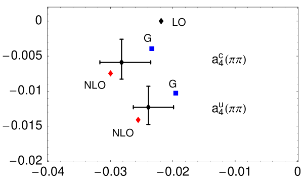
Figure 4: LO, NLO and NLO_sp value of $a_{4}^{p}$ in the complex plane. $a_{4}^{u}$ has a sizeable phase. The NLO_sp point includes a theoretical error estimate.

A graphical representation of 1-loop corrections to $a^{p}_{4}$ is given in Figure 4. The leading-order (LO) point corresponds to naive factorization. The point labelled “NLO” includes all $\alpha_{s}$ corrections. The point including the error bars is the result of our calculation that adds the 1-loop spectator-scattering correction. We refer to this partial next-to-next-to-leading order (NNLO) calculation as “NLO_sp”, since the NNLO term is a 1-loop correction in the spectator-scattering sector. The point “G” corresponds to a choice of inputs made in [4] to achieve an improved agreement with the $B\to\pi\pi$ decay rates. This input parameter set uses $\lambda_{B}=200\,\mbox{MeV}$ and $a_{2}^{\pi}=0.3$ near the boundaries of the assumed regions instead of the central values given in Table 2, which leads to an increase of the spectator-scattering contribution.

The figure shows that the new correction has a small effect on the real part, but can be relevant to the imaginary part depending on parameter values. As was found in [4] for the parameters $a_{1},a_{2}$, perturbation theory is well-behaved. These observations apply to all final states, in particular, “non-factorizable” SU(3) breaking turns out to be quite small, as discussed above.

To gauge the impact of the spectator-scattering correction on branching fractions and CP asymmetries, we recall that $a_{4}^{p}$ always appears in conjunction with the power-suppressed penguin amplitude $r_{\chi}a_{6}^{p}$. Since we have not computed 1-loop corrections to the short-distance coefficients of power-suppressed operators, the value of $r_{\chi}a_{6}^{p}$ differs from previous analyses only due to the updated input parameters. Furthermore, since the tree-level spectator scattering contribution vanishes for $a_{6}^{p}$, the following numbers are solely due to the naive-factorization and 1-loop contributions to the form-factor term in the factorization formula. We have

$$r_{\chi}^{\pi}a_{6}^{u}(\pi\pi) = -0.055-[0.001]_{V}-[0.004+0.020i]_{P}$$ (100)

$$= -0.060^{+0.011}_{-0.017}+(-0.020^{+0.005}_{-0.006})i,\qquad$$

$$r_{\chi}^{\pi}a_{6}^{c}(\pi\pi) = -0.055-[0.001]_{V}-[0.009+0.010i]_{P}$$ (101)

$$= -0.065^{+0.012}_{-0.019}+(-0.010^{+0.004}_{-0.004})i.\qquad$$

It is worth noting that $r_{\chi}^{\pi}a_{6}^{p}(\pi\pi)$ is numerically larger than $a^{p}_{4}(\pi\pi)$. On the other hand, $r_{\chi}^{\pi}a_{6}^{p}(M_{1}M_{2})$ is strongly suppressed when $M_{2}$ is a vector meson, where the naive-factorization contribution is zero. We shall discuss some of the phenomenology associated with the penguin amplitudes in Section 5.

4.3.3 The flavour-singlet QCD penguin amplitude $\alpha_{3}^{p}$

The flavour-singlet QCD penguin amplitude is not relevant to the $\pi\pi$ final state. We therefore give numerical values for

$$a_{3}^{p}(\bar{K}\phi) = 0.001+[0.005+0.002i]_{V}$$ (102)

$$-\left[\frac{r_{\rm sp}}{0.435}\right]\Big{\{}[0.003]_{\rm LO}+[0.001+0.001i]_{HV}+[0.002]_{\rm tw3}\Big{\}}$$

$$= 0.001^{+0.004}_{-0.005}+(0.001^{+0.002}_{-0.003})i,$$

$$a_{5}^{p}(\bar{K}\phi) = -0.005-[0.002+0.003i]_{V}$$ (103)

$$+\left[\frac{r_{\rm sp}}{0.435}\right]\Big{\{}[0.004]_{\rm LO}+[0.002+0.002i]_{HV}+[0.002]_{\rm tw3}\Big{\}}$$

$$= 0.001^{+0.007}_{-0.004}+(-0.000^{+0.005}_{-0.003})i,$$

valid for $p=u$ and $p=c$. Here the 1-loop spectator scattering term “$HV$” is numerically of the same size as the other terms, and gives a large effect. This is typical for corrections to the smaller colour-suppressed amplitudes. We recall from Section 2 that the calculation of the flavour-singlet amplitudes $a^{p}_{3,5}$ is not complete when $M_{2}$ is a pseudoscalar meson, since we did not compute the matching coefficients of two-gluon operators. Even more important conceptually, there is another term in the QCD factorization formula which does not factorize in the form of (1), which has been estimated to be of similar size as the individual terms in (102), (103) [12], but which is very uncertain.

Because the flavour-singlet amplitude $\alpha_{3}^{p}=a_{3}\mp a_{5}$ is so small, it does not play an important role in the phenomenology of the more prominent charmless final states, in particular in the explanation of the large $\eta^{\prime}K$ branching fractions [12]. The large spectator-scattering correction found above affects final states such as $\eta^{\prime}K^{*}$ or such with very small branching fractions, where the leading contribution from $\alpha_{4}^{p}$ is suppressed. However, the predictions for such decays carry large theoretical uncertainties.

4.3.4 Electroweak penguin amplitudes

The electroweak (EW) penguin amplitudes are small, yet they contribute significantly to isospin-breaking effects in decays to $\pi K$ final states. The “colour-allowed” EW penguin amplitude is $\alpha_{3,\rm EW}^{p}=a_{9}^{p}\mp a_{7}^{p}$ (upper sign for $\pi K$). We find

$$a_{7}^{u}(\bar{K}\pi) = 10^{-2}\times\Bigg{(}0.009+[0.002+0.003i]_{V}+[0.038]_{P}$$ (104)

$$-\left[\frac{r_{\rm sp}}{0.435}\right]\Big{\{}[0.005]_{\rm LO}+[0.003+0.004i]_{HV}-[0.020+0.016i]_{HP}+[0.003]_{\rm tw3}\Big{\}}\Bigg{)}$$

$$=10^{-2}\times\Big{(}0.058^{+0.024}_{-0.017}+(0.015^{+0.010}_{-0.006})i\Big{)},$$

$$a_{7}^{c}(\bar{K}\pi) = 10^{-2}\times\Bigg{(}0.009+[0.002+0.003i]_{V}+[0.011]_{P}$$ (105)

$$-\left[\frac{r_{\rm sp}}{0.435}\right]\Big{\{}[0.005]_{\rm LO}+[0.003+0.004i]_{HV}+[0.002-0.001i]_{HP}+[0.003]_{\rm tw3}\Big{\}}\Bigg{)}$$

$$=10^{-2}\times\Big{(}0.010^{+0.011}_{-0.017}+(0.000^{+0.003}_{-0.006})i\Big{)},$$

$$a_{9}^{u}(\bar{K}\pi) = 10^{-2}\times\Bigg{(}-0.909-[0.023+0.011i]_{V}+[0.038]_{P}$$ (106)

$$+\left[\frac{r_{\rm sp}}{0.435}\right]\Big{\{}[0.017]_{\rm LO}+[0.028+0.025i]_{HV}+[0.020+0.016i]_{HP}+[0.010]_{\rm tw3}\Big{\}}\Bigg{)}$$

$$=10^{-2}\times\Big{(}-0.819^{+0.080}_{-0.042}+(0.029^{+0.053}_{-0.023})i\Big{)},$$

$$a_{9}^{c}(\bar{K}\pi) = 10^{-2}\times\Bigg{(}-0.909-[0.023+0.011i]_{V}+[0.011]_{P}$$ (107)

$$+\left[\frac{r_{\rm sp}}{0.435}\right]\Big{\{}[0.017]_{\rm LO}+[0.028+0.025i]_{HV}-[0.002-0.001i]_{HP}+[0.010]_{\rm tw3}\Big{\}}\Bigg{)}$$

$$=10^{-2}\times\Big{(}-0.868^{+0.058}_{-0.026}+(0.015^{+0.043}_{-0.018})i\Big{)}.$$

The penguin-contraction term “$HP$” originates from the diagrams shown in the third line of Figure 3. Both “$P$” and “$HP$” coincide for $a_{7}^{p}$ and $a_{9}^{p}$, such that they exactly cancel in the combination $a_{9}-a_{7}$ appropriate to final states with pseudoscalar $M_{2}$, but add up for vector $M_{2}$. The 1-loop spectator scattering correction is quite important for $a_{7}^{p}$, and $a_{7}^{u}$ is seen to even be dominated by the penguin contractions. However, what is relevant to decay amplitudes is $\alpha_{3,\rm EW}$, and therein the 1-loop corrections are overwhelmed by the large tree contribution to $a_{9}^{p}$.

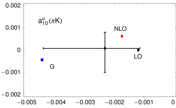
Figure 5: The electroweak penguin amplitude $a^{p}_{10}$ receives a large correction. The amplitude is almost identical for $p=u$ and $p=c$, therefore only the case $p=u$ is shown.

The colour-suppressed EW penguin amplitude $\alpha_{4,\rm EW}^{p}=a_{10}^{p}\pm r_{\chi}a_{8}^{p}$ consists of $a_{10}^{p}$ and a power-suppressed amplitude $r_{\chi}a_{8}^{p}$, which is the electroweak equivalent to $r_{\chi}a_{6}^{p}$. We find

$$r_{\chi}^{\bar{K}}a_{8}^{u}(\pi\bar{K}) = 10^{-2}\times\Bigg{(}0.063+[0.000]_{V}+[0.004-0.016i]_{P}\Bigg{)}$$ (108)

$$= 10^{-2}\times\Big{(}0.068^{+0.025}_{-0.024}+(-0.016^{+0.010}_{-0.012})i\Big{)},$$

$$r_{\chi}^{\bar{K}}a_{8}^{c}(\pi\bar{K}) = 10^{-2}\times\Bigg{(}0.063+[0.000]_{V}+[0.002-0.010i]_{P}\Bigg{)}$$ (109)

$$= 10^{-2}\times\Big{(}0.065^{+0.025}_{-0.025}+(-0.010^{+0.006}_{-0.007})i\Big{)},$$

$$a_{10}^{u}(\pi\bar{K}) = 10^{-2}\times\Bigg{(}-0.161+[0.135+0.073i]_{V}+[0.026-0.011i]_{P}$$ (110)

$$-\left[\frac{r_{\rm sp}}{0.485}\right]\Big{\{}[0.115]_{\rm LO}+[0.050+0.051i]_{HV}+[0.007+0.004i]_{HP}+[0.061]_{\rm tw3}\Big{\}}\Bigg{)}$$

$$=10^{-2}\times\Big{(}-0.233^{+0.119}_{-0.210}+(0.008^{+0.073}_{-0.107})i\Big{)},$$

$$a_{10}^{c}(\pi\bar{K}) = 10^{-2}\times\Bigg{(}-0.161+[0.135+0.073i]_{V}+[0.023-0.006i]_{P}$$ (111)

$$-\left[\frac{r_{\rm sp}}{0.485}\right]\Big{\{}[0.115]_{\rm LO}+[0.050+0.051i]_{HV}+[0.002-0.001i]_{HP}+[0.061]_{\rm tw3}\Big{\}}\Bigg{)}$$

$$=10^{-2}\times\Big{(}-0.231^{+0.118}_{-0.207}+(0.017^{+0.071}_{-0.105})i\Big{)}.$$

The coefficient $a_{10}^{p}$ is similar to the colour-suppressed tree amplitude $a_{2}$. The non-spectator term (first line in each expression) is strongly suppressed due to a cancellation between the naive-factorization term and the 1-loop correction, which is large due to the absence of colour-suppression. The final number is largely from spectator-scattering which obtains significant 1-loop corrections. The result is displayed graphically in Figure 5.

5 Amplitude ratios

With the improved $a_{i}^{p}$ parameters we are in a position to calculate complex ratios of strong amplitudes such as $P/T$ or $C/T$. In this section we discuss a few prominent examples.

5.1 The $PP$, $PV$, $V\!P$, and $[VV]_{L}$ QCD penguin amplitude

     

     

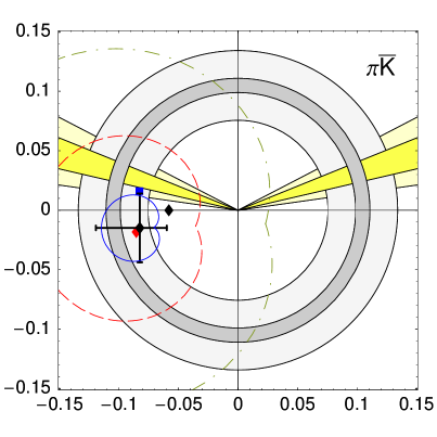
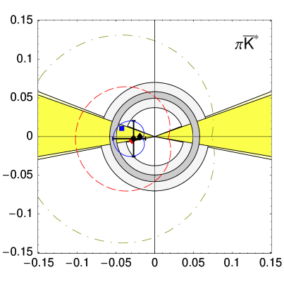
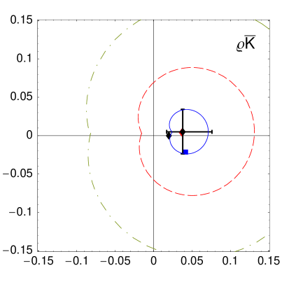
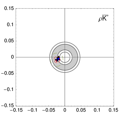
Figure 6: Comparing the $PP$, $PV$, $VP$, and $VV$ penguin amplitudes to data. The figures in the upper row show theory predictions for $\hat{\alpha}_{4}^{c}(M_{1}M_{2})/(\alpha_{1}(\pi\pi)+\alpha_{2}(\pi\pi))$; those in the lower row show $\hat{\alpha}_{4}^{c}(M_{1}M_{2})/(\alpha_{1}(\rho\rho)+\alpha_{2}(\rho\rho))$. Where available, the ranges for modulus and phase extracted from data are also depicted. See text for explanations.

We recall that in physical decay amplitudes the parameters $a_{4}^{p}$, $a_{6}^{p}$, and the penguin annihilation amplitude $\beta_{3}^{p}$ always appear in the same linear combination [9]

$$\hat{\alpha}_{4}^{p}(M_{1}M_{2})=a_{4}(M_{1}M_{2})\pm r_{\chi}^{M_{2}}a_{6}(M_{1}M_{2})+\beta_{3}^{p}(M_{1}M_{2}),$$ (112)

where the upper (lower) sign corresponds to the case $M_{1}=P\,(V)$, and cannot individually be confronted with experiment. The annihilation contribution $\beta_{3}^{p}$ is incalculable in factorization, since it contains an endpoint divergence; we therefore resort to the model defined in [2], parameterizing it in terms of a complex parameter

$$X_{A}=\ln\frac{m_{B}}{\Lambda_{h}}\,(1+\varrho_{A}e^{i\phi_{A}})$$ (113)

with $\Lambda_{h}=500\,\mbox{MeV}$ a hadronic scale and $\varrho_{A}=0$ by default. An additional theoretical error is assigned to any observable by setting $\varrho_{A}=1$ and allowing the phase $\phi_{A}$ to take arbitrary values. It turns out that this is almost always by far the largest theoretical uncertainty for direct CP asymmetries, and among the largest uncertainties for branching fractions of penguin-dominated decays, especially those with vector mesons in the final state. The expressions for the annihilation amplitudes are given in [9] and, for $VV$ final states, in [28].

To assess the validity of the QCD factorization framework, we show in Figure 6 the ratios $\hat{\alpha}_{4}^{c}(M_{1}M_{2})/(\alpha_{1}(\pi\pi)+\alpha_{2}(\pi\pi))$ ($M_{1}M_{2}=\pi\bar{K},\,\pi\bar{K}^{*}$) and $\hat{\alpha}_{4}^{c}(M_{1}M_{2})/(\alpha_{1}(\rho\rho)+\alpha_{2}(\rho\rho))$ ($M_{1}M_{2}=\rho\bar{K},\,\rho\bar{K}^{*}$), the first two of which have been previously considered in [9]. (For $\rho\bar{K}^{*}$ and $\rho\rho$, only the longitudinal polarization amplitude is considered in the following.) The result of the calculation is represented by the dark point with error bars. The nearly circular contours around this point show the variation of the theoretical prediction when the phase of the annihilation model is varied from 0 to $2\pi$ for fixed $\varrho_{A}=1,2,3$ (inner to outer circles). The blue square corresponds to the parameter set G, which is defined by $\lambda_{B}=200\,\mbox{MeV}$, $a_{2}^{\pi}=0.3$, $m_{s}=80\,\mbox{MeV}$, $\varrho_{A}=1$ and $\phi_{A}=-55^{\circ}\,(PP)$, $\phi_{A}=-20^{\circ}\,(PV)$, $\phi_{A}=-70^{\circ}\,(VP)$, $\varrho_{A}=0$ ($VV$), following the favoured parameter set S4 of [9].

As far as data is available, the amplitude ratios can be obtained with little theory input from the well measured (CP-averaged, longitudinal) branching fractions $\mbox{Br}(B^{-}\to\pi^{-}\bar{K}^{(*)0})$, $f_{L}(\rho^{-}\bar{K}^{*0})\cdot\mbox{Br}(B^{-}\to\rho^{-}\bar{K}^{*0})$, $\mbox{Br}(B^{-}\to\pi^{-}\pi^{0})$, $f_{L}(\rho^{-}\rho^{0})\cdot\mbox{Br}(B^{-}\to\rho^{-}\rho^{0})$, and the rate and direct CP asymmetry in $\bar{B}^{0}\to\pi^{+}K^{(*)-}$ (cf. [9], (75) and (77)). The darker rings are due to the experimental errors in the branching fractions and the lighter ones include also the uncertainty of $|V_{ub}|$. The angles of the wedges involve the CP asymmetry measurements (darker region) while the lighter region also includes the error on $\gamma$. The wedges opening to the right are ruled out (or at least disfavoured) by the fact that the measured values of the Fleischer-Mannel ratios [29]

$$R_{\rm FM}^{\pi K}=\frac{\Gamma(\bar{B}^{0}\to\pi^{+}K^{-})}{\Gamma(B^{-}\to\pi^{-}\bar{K}^{0})}=0.91\pm 0.07,\qquad R_{\rm FM}^{\pi K^{*}}=\frac{\Gamma(\bar{B}^{0}\to\pi^{+}K^{*-})}{\Gamma(B^{-}\to\pi^{-}\bar{K}^{*0})}=0.93\pm 0.19$$ (114)

are both less than unity.

Three messages can be read off from the figure. (1) The magnitudes and phases predicted for the amplitude ratios agree reasonably well with data, as indicated by the error bars and the small onion-shaped regions. A large annihilation amplitude is disfavoured, since it would require fine-tuning of the phase to satisfy the experimental constraints, but some annihilation contribution appears to be required, especially for the $PV$ amplitude. (The apparent smallness of the annihilation uncertainty in the $\rho\bar{K}^{*}$ plot is due to cancellations in the crude annihilation model employed here.) There is a tendency of the predicted magnitude of the penguin amplitude without annihilation to be smaller than the data. This difference is about $0.02$ to $0.03$ independent of the spins of the final-state mesons, except for the $VV$ final state where no such difference exists. (2) The magnitude of the penguin amplitude is predicted much smaller in the case containing a vector meson in the final state, either due to the smallness of $a^{p}_{6}$ ($\pi K^{*},\,\rho K^{*}$) or a cancellation of $a^{p}_{4}$ and $a^{p}_{6}$ ($\rho K$). This is also reflected by the data. (3) A priori the ratio could have lain anywhere in the complex plane shown in the figure. The agreement found hence constitutes a highly non-trivial check of the qualitative and quantitative predictions for penguin amplitudes in the factorization framework. In this graphical representation the well-known difficulty to account for the small direct CP asymmetry in $\bar{B}^{0}\to\pi^{+}K^{-}$ in QCD factorization is seen as a small offset of the theoretical calculation from the left wedge in the first panel of the figure.

5.2 $P/T$ and $C/T$

Penguin-to-tree and other ratios are also of phenomenological importance in $B\to\pi\pi$, $B\to\pi\rho$, $B\to\rho\rho$, and other decays. The ratio $P_{\pi\pi}/T_{\pi\pi}$, for instance, can be determined solely from the time-dependent CP asymmetry in $B\to\pi^{+}\pi^{-}$ for given values of the well measured mixing phase $\phi_{d}$, equal to $2\beta$ in the Standard Model, and the CKM angle $\gamma$. Conversely theoretical predictions for these ratios allow to extract the angle $\gamma$. Similar relations hold for final states $\pi^{\mp}\rho^{\pm}$, $\rho^{+}\rho^{-}$, $\pi^{+}K^{(*)-}$, etc. Here we present numerical values for a number of these ratios.

Ratio	Value/Range	Value G
$\displaystyle\frac{P_{\pi\pi}}{T_{\pi\pi}}$	$-0.122^{+0.033}_{-0.063}+(-0.024^{+0.047}_{-0.048})i$	$-0.162+0.022i$
$\displaystyle\frac{P_{\rho\rho}}{T_{\rho\rho}}$	$-0.036^{+0.006}_{-0.009}+(-0.009^{+0.007}_{-0.007})i$	$-0.037-0.009i$
$\displaystyle\frac{P_{\pi\rho}}{T_{\pi\rho}}$	$-0.037^{+0.015}_{-0.028}+(-0.005^{+0.024}_{-0.024})i$	$-0.070+0.006i$
$\displaystyle\frac{P_{\rho\pi}}{T_{\rho\pi}}$	$0.042^{+0.039}_{-0.023}+(0.004^{+0.030}_{-0.030})i$	$\phantom{-}0.051-0.024i$
$\displaystyle\frac{C_{\pi\pi}}{T_{\pi\pi}}$	$0.363^{+0.277}_{-0.156}+(0.029^{+0.166}_{-0.103})i$	$\phantom{-}0.691+0.165i$
$\displaystyle\frac{C_{\rho\rho}}{T_{\rho\rho}}$	$\phantom{-}0.198^{+0.233}_{-0.150}+(-0.009^{+0.145}_{-0.097})i$	$\phantom{-}0.344+0.042i$
$\displaystyle\frac{C_{\pi\rho}}{T_{\pi\rho}}$	$\phantom{-}0.250^{+0.229}_{-0.143}+(-0.012^{+0.127}_{-0.090})i$	$\phantom{-}0.467+0.071i$
$\displaystyle\frac{C_{\rho\pi}}{T_{\rho\pi}}$	$\phantom{-}0.134^{+0.199}_{-0.156}+(-0.024^{+0.152}_{-0.117})i$	$\phantom{-}0.283+0.138i$
$\displaystyle\frac{T_{\rho\pi}}{T_{\pi\rho}}$	$0.869^{+0.275}_{-0.207}+(0.014^{+0.058}_{-0.057})i$	$\phantom{-}0.945-0.004i$

Table 3: Amplitude ratios for the $\pi\pi$, $\rho\rho$ and $\pi\rho$ final states. In the case of $\rho\rho$ the ratios of longitudinal polarization amplitudes are given. The third column gives the preferred-parameter-set G value.

In such phenomenological studies it is convenient to define the colour-allowed tree amplitude $T$, the colour-suppressed tree amplitude $C$, and the penguin amplitude $P$ as the hadronic amplitudes multiplying the different CKM structures in the decay amplitude. In this convention, the name of an amplitude derives from its leading contribution, such that $T\sim\alpha_{1}$, $C\sim\alpha_{2}$, and $P\sim\alpha_{4}^{c}$, but sub-leading terms can make an important difference. For the following discussion of $B\to\pi\pi,\rho\rho,\pi\rho$ decays, we define $T,C,P$ through

$${\cal A}_{\overline{B}^{0}\to\pi^{+}\rho^{-}} \propto V^{*}_{ud}V_{ub}T_{\pi\rho}+V^{*}_{cd}V_{cb}P_{\pi\rho},$$

$${\cal A}_{\overline{B}^{0}\to\pi^{-}\rho^{+}} \propto V^{*}_{ud}V_{ub}T_{\rho\pi}+V^{*}_{cd}V_{cb}P_{\rho\pi},$$

$$-2{\cal A}_{\overline{B}^{0}\to\pi^{0}\rho^{0}} \propto V^{*}_{ud}V_{ub}[C_{\pi\rho}+C_{\rho\pi}]+V^{*}_{cd}V_{cb}[\ldots].$$ (115)

These definitions are related to the $\alpha_{i}^{p}$ (and annihilation) amplitudes by comparing the above equations to [9], (A.13). The proportionality factor is the same in all three lines and therefore irrelevant, since we shall only consider ratios. Analogous definitions apply to $\pi\pi$ and $\rho\rho$.

Our results for the amplitude ratios are given in Table 3. The first column of numbers provides the default result with errors, the second column the value in parameter set G that we currently consider as our “best” result. The theoretical calculation has significant uncertainties. The dominant error of $P/T$ always arises from the weak annihilation model and cannot be reduced by further calculations. The error due to neglected higher-order corrections is difficult to estimate, but there may be a sizable shift of the central values of $P/T$ due to the uncalculated ${\cal O}(\alpha_{s}^{2})$ correction to the power-suppressed “scalar penguin” amplitude $a_{6}^{p}$. That correction, like $a_{4}^{p}$ discussed above, involves the large Wilson coefficient $C_{1}$ at one loop, but there may not be a numerical cancellation analogous to the one observed for $a_{4}^{p}$ in Section 4.3.2. For $C/T$, insufficiently known input parameters such as $\lambda_{B}$ and $a_{2}^{M}$, and to a lesser extent the twist-3 correction $X_{H}$, are responsible for the bulk of the uncertainty.

There is a clear hierarchy of the penguin-to-tree ratios that has already been discussed in [9] and in the previous subsection. The difference in $C/T$ for the various final states is in fact a reflection of the same hierarchy of penguin amplitudes. While $a_{1,2}$ are roughly the same for $\pi\pi$, $\pi\rho$, $\rho\rho$ (longitudinal polarization), the amplitudes $T,C$ contain the up-penguin amplitude, such that $T=\alpha_{1}+\alpha_{4}^{u}+\ldots$,   $C=\alpha_{2}-\alpha_{4}^{u}+\ldots$. It is worth noting that $C/T$ can acquire a significant imaginary part from the 1-loop vertex and spectator-scattering correction, and the large phase of the up-penguin amplitude. It will be interesting to detect these characteristic features in the experimental data.

5.3 Relating electroweak penguin to tree amplitudes

The electroweak penguin amplitudes $\alpha^{p}_{3,\rm EW}$, $\alpha^{p}_{4,\rm EW}$ are related to the tree amplitudes $\alpha_{1,2}$ under certain assumptions [30, 31, 32]. Therefore, more than the calculated values of the electroweak amplitudes, the deviations from these relations are of interest. The assumptions made in deriving the relations are the neglect of the electroweak penguin operators $Q_{7,8}$, since they have small Wilson coefficient compared to $Q_{9,10}$ at the scales of interest, and SU(3) flavour symmetry, when a relation between $\pi\pi$ and $\pi K$ final states is involved. In addition there are further assumptions, which amount to neglecting the charm and bottom content of the operators $Q_{9,10}$, and to not considering penguin contractions. Since our calculation does not make use of any of these assumptions, it is interesting to investigate how well these widely used amplitude relations are satisfied. We confine ourselves to the discussion of the $\pi K$ and $\pi\pi$ final states.

The most solid relation is [30]

$$\delta_{\mathrm{EW}}=-\frac{3}{2}\left|\frac{V^{*}_{cs}V_{cb}}{V^{*}_{us}V_{ub}}\right|\frac{R_{\pi K}\alpha^{c}_{3,\rm EW}(\bar{K}\pi)+\alpha^{c}_{4,\rm EW}(\pi\bar{K})}{\alpha_{1}(\pi\pi)+\alpha_{2}(\pi\pi)}\approx-\frac{3}{2}\left|\frac{V^{*}_{cs}V_{cb}}{V^{*}_{us}V_{ub}}\right|\frac{C_{9}+C_{10}}{C_{1}+C_{2}}$$ (116)

with $R_{\pi K}=f_{\pi}F^{BK}(0)/(f_{K}F^{B\pi}(0))$ and a similar relation with $\pi\pi$ in the numerator and $R_{\pi K}\to 1$. Let ${\cal R}_{\rm NR}$ be the ratio of the middle expression to the right-hand side. We find

$${\cal R}_{\rm NR}=(1.02^{+0.27}_{-0.22})\,e^{i(1\pm 1)^{\circ}}$$ (117)

The closeness to 1 involves a cancellation between an SU(3) breaking on the order of $10\%$ and an error of similar size due to neglecting the electroweak penguin operators $Q_{7,8}$ (for $\pi\pi$ we would find ${\cal R}_{\rm NR}\approx(0.92^{+0.05}_{-0.04})\,e^{i(1\pm 1)^{\circ}}$). The effect of penguin contractions is below the $(1-2)\%$ level. Note also that the ratio remains real to an excellent approximation. The relation holds to much better accuracy than at the time when [2] was written, where it was studied without the 1-loop spectator scattering correction. The difference with respect to [2] is almost exclusively due to the change in the hadronic parameter ratio $R_{\pi K}$, which is also responsible for the bulk of the error.

A second relation follows from SU(3) symmetry [31], which also involves annihilation amplitudes. Neglecting such power-suppressed amplitudes, we obtain

$$\frac{R_{\pi K}\alpha^{c}_{3,\rm EW}(\bar{K}\pi)-\alpha^{c}_{4,\rm EW}(\pi\bar{K})}{\alpha_{1}(\pi\pi)-\alpha_{2}(\pi\pi)}=\frac{C_{9}-C_{10}}{C_{1}-C_{2}}$$ (118)

Let ${\cal R}_{\rm GPY}$ be the ratio of the left-hand to the right-hand side. We find

$${\cal R}_{\rm GPY}=(1.29^{+0.58}_{-0.38})\,e^{i(-1^{+3}_{-2})^{\circ}}$$ (119)

The deviation from 1, which is bigger than in ${\cal R}_{\rm NR}$, comes about because now the SU(3)-breaking correction (for $\pi\pi$ we would find ${\cal R}_{\rm GPY}\approx 1.13$) and the effect of neglecting $C_{7,8}$ add up. Individually, both effects are nearly twice as large as in the first relation, which is also reflected in the larger error. Nevertheless, ${\cal R}_{\rm GPY}$ remains real to an excellent approximation.

The previous two relations (116), (118) hold under the stated assumptions irrespective of the values of the Wilson coefficients $C_{9,10}$. Observing that

$$\frac{C_{9}+C_{10}}{C_{1}+C_{2}}\approx\frac{C_{9}-C_{10}}{C_{1}-C_{2}}\approx-0.00896\equiv\kappa,$$ (120)

at $\mu_{b}=4.8\,\mbox{GeV}$ and neglecting the $1\%$ difference between the first three items in this expression, stronger relations are obtained in [31],

$$\alpha^{c}_{3,\rm EW}=\kappa\alpha_{1},\qquad\alpha^{c}_{4,\rm EW}=\kappa\alpha_{2},$$ (121)

where due to the SU(3)-symmetry assumption the arguments $M_{1}M_{2}$ of the $\alpha_{i}$ can be any out of $\pi\pi$, $\pi\bar{K}$, $\bar{K}\pi$ and $K\bar{K}$, $\bar{K}K$. The first of these relations is extraordinarily well respected,

$$\frac{\alpha^{c}_{3,\rm EW}(\pi\pi)}{\kappa\alpha_{1}(\pi\pi)}=(1.00\pm 0.01)\,e^{i(0^{+0}_{-1})^{\circ}},$$ (122)

because it involves the colour-allowed amplitudes, and the effect of $Q_{7,8}$ is very small. This holds for any of the above final states $\pi\pi,\pi K,KK$. In contrast, the second relation between the colour-suppressed amplitudes is poor. We find

$$\frac{\alpha^{c}_{4,\rm EW}(\pi\pi)}{\kappa\alpha_{2}(\pi\pi)}=(0.64^{+0.25}_{-0.24})\,e^{i(3^{+11}_{-14})^{\circ}}.$$ (123)

Our theoretical expectations should be useful to estimate the error incurred by employing these relations in data-driven approaches to non-leptonic decays.

6 Conclusion

This paper, together with [4], completes the calculation of 1-loop spectator-scattering corrections to all flavour-nonsinglet, leading-power decay amplitudes in non-leptonic $B$ decays. The calculation shows that factorization works technically: the infrared singularities cancel in the matching calculation, and the convolution integrals converge at their endpoints.

The 1-loop corrections are numerically well-behaved. As a general rule, we find significant effects for the colour-suppressed amplitudes $\alpha_{2}$, $\alpha_{3}^{p}$ and $\alpha^{p}_{4,\rm EW}$, and small effects for the others. In case of the QCD penguin amplitude $a_{4}^{p}$ this conclusion is reached only as the result of a numerical cancellation in the terms proportional to the large Wilson coefficient $C_{1}$. As a consequence, there is little impact of the newly calculated spectator-scattering corrections to penguin amplitudes on the phenomenology of non-leptonic branching fractions and CP asymmetries. Further improvement of the calculation now requires the calculation of the 2-loop vertex corrections to the form-factor term in the factorization formula [33], and an understanding of the power-suppressed but large penguin amplitude $a_{6}^{p}$.

In the final section of the paper we investigated a few amplitude ratios that play an important role in determining $\gamma$ ($\alpha$) from tree-dominated $b\to d$ transitions. Vice versa, assuming a value of $\gamma$, these ratios may be determined from data and compared to the theoretical calculation. A detailed discussion of branching fractions and CP asymmetries with account of 1-loop spectator scattering will be presented elsewhere.

Acknowledgements

This work is supported in part by the DFG Sonderforschungsbereich/Transregio 9 “Computergestützte Theoretische Teilchenphysik”.

References

-
[1]
M. Beneke, G. Buchalla, M. Neubert and C. T. Sachrajda,
Phys. Rev. Lett. 83 (1999) 1914
[hep-ph/9905312];
M. Beneke, G. Buchalla, M. Neubert and C. T. Sachrajda, Nucl. Phys. B 591 (2000) 313 [hep-ph/0006124]. - [2] M. Beneke, G. Buchalla, M. Neubert and C. T. Sachrajda, Nucl. Phys. B 606 (2001) 245 [hep-ph/0104110].
-
[3]
J. Chay and C. Kim,
Nucl. Phys. B 680 (2004) 302
[hep-ph/0301262];
C. W. Bauer, D. Pirjol, I. Z. Rothstein and I. W. Stewart, Phys. Rev. D 70 (2004) 054015 [hep-ph/0401188]. - [4] M. Beneke and S. Jäger, Nucl. Phys. B 751 (2006) 160 [hep-ph/0512351].
-
[5]
R. J. Hill, T. Becher, S. J. Lee and M. Neubert,
JHEP 0407 (2004) 081
[hep-ph/0404217];
T. Becher and R. J. Hill, JHEP 0410 (2004) 055 [hep-ph/0408344];
G. G. Kirilin, [hep-ph/0508235]. - [6] M. Beneke and D. Yang, Nucl. Phys. B 736 (2006) 34 [hep-ph/0508250].
- [7] X. q. Li and Y. d. Yang, Phys. Rev. D 72 (2005) 074007 [hep-ph/0508079].
-
[8]
A. J. Buras, M. Jamin, M. E. Lautenbacher and P. H. Weisz,
Nucl. Phys. B 400 (1993) 37
[hep-ph/9211304];
M. Ciuchini, E. Franco, G. Martinelli and L. Reina, Nucl. Phys. B 415 (1994) 403 [hep-ph/9304257]. - [9] M. Beneke and M. Neubert, Nucl. Phys. B 675 (2003) 333 [hep-ph/0308039].
-
[10]
L. L. Chau, H. Y. Cheng, W. K. Sze, H. Yao and B. Tseng,
Phys. Rev. D 43 (1991) 2176;
M. Gronau, O. F. Hernandez, D. London and J. L. Rosner, Phys. Rev. D 50 (1994) 4529 [hep-ph/9404283]. - [11] M. Beneke, J. Rohrer and D. Yang, Phys. Rev. Lett. 96 (2006) 141801 [hep-ph/0512258].
- [12] M. Beneke and M. Neubert, Nucl. Phys. B 651 (2003) 225 [hep-ph/0210085].
-
[13]
M. Beneke, A. P. Chapovsky, M. Diehl and Th. Feldmann,
Nucl. Phys. B 643 (2002) 431
[hep-ph/0206152];
M. Beneke and Th. Feldmann, Phys. Lett. B 553 (2003) 267 [hep-ph/0211358]. - [14] A. R. Williamson and J. Zupan, Phys. Rev. D 74 (2006) 014003 [hep-ph/0601214].
- [15] E. Baracchini and G. Isidori, Phys. Lett. B 633 (2006) 309 [hep-ph/0508071].
- [16] D. s. Du, D. s. Yang and G. h. Zhu, Phys. Lett. B 488 (2000) 46 [hep-ph/0005006].
-
[17]
C. W. Bauer, S. Fleming, D. Pirjol and I. W. Stewart,
Phys. Rev. D 63 (2001) 114020
[hep-ph/0011336];
C. W. Bauer, D. Pirjol and I. W. Stewart, Phys. Rev. D 65 (2002) 054022 [hep-ph/0109045];
R. J. Hill and M. Neubert, Nucl. Phys. B 657 (2003) 229 [hep-ph/0211018]. - [18] M. Beneke and T. Feldmann, Nucl. Phys. B 685 (2004) 249 [hep-ph/0311335].
-
[19]
C. W. Bauer, D. Pirjol and I. W. Stewart,
Phys. Rev. D 67 (2003) 071502
[hep-ph/0211069];
B. O. Lange and M. Neubert, Nucl. Phys. B 690 (2004) 249 [Erratum-ibid. B 723 (2005) 201] [hep-ph/0311345]. - [20] M. Beneke and V. A. Smirnov, Nucl. Phys. B 522 (1998) 321 [hep-ph/9711391].
- [21] N. Kivel, [hep-ph/0608291].
- [22] J. C. Collins, A. V. Manohar and M. B. Wise, Phys. Rev. D 73 (2006) 105019.
- [23] A. Khodjamirian, T. Mannel and M. Melcher, Phys. Rev. D 70 (2004) 094002 [hep-ph/0407226].
-
[24]
V. M. Braun and A. Lenz,
Phys. Rev. D 70 (2004) 074020
[hep-ph/0407282];
P. Ball and R. Zwicky, Phys. Lett. B 633 (2006) 289 [hep-ph/0510338];
P. Ball, V. M. Braun and A. Lenz, JHEP 0605 (2006) 004 [hep-ph/0603063];
V. M. Braun et al., Phys. Rev. D 74 (2006) 074501 [hep-lat/0606012];
P. A. Boyle et al. [UKQCD Collaboration], Phys. Lett. B 641 (2006) 67 [hep-lat/0607018]. -
[25]
V. M. Braun, D. Y. Ivanov and G. P. Korchemsky,
Phys. Rev. D 69 (2004) 034014
[hep-ph/0309330];
A. Khodjamirian, T. Mannel and N. Offen, Phys. Lett. B 620 (2005) 52 [hep-ph/0504091];
A. G. Grozin and M. Neubert, Phys. Rev. D 55 (1997) 272 [hep-ph/9607366];
S. J. Lee and M. Neubert, Phys. Rev. D 72 (2005) 094028 [hep-ph/0509350]. - [26] P. Ball and R. Zwicky, Phys. Rev. D 71 (2005) 014015 [hep-ph/0406232].
-
[27]
G. P. Lepage and S. J. Brodsky,
Phys. Rev. D 22 (1980) 2157;
A. V. Efremov and A. V. Radyushkin, Phys. Lett. B 94 (1980) 245. -
[28]
A. L. Kagan,
Phys. Lett. B 601 (2004) 151
[hep-ph/0405134];
J. Rohrer, Diploma Thesis, RWTH Aachen, 2004. - [29] R. Fleischer and T. Mannel, Phys. Rev. D 57 (1998) 2752 [hep-ph/9704423].
- [30] M. Neubert and J. L. Rosner, Phys. Lett. B 441 (1998) 403 [hep-ph/9808493].
- [31] M. Gronau, D. Pirjol and T. M. Yan, Phys. Rev. D 60 (1999) 034021 [hep-ph/9810482].
- [32] A. J. Buras and R. Fleischer, Eur. Phys. J. C 11 (1999) 93 [hep-ph/9810260].
- [33] Results for the imaginary parts of the tree amplitudes have been presented by G. Bell, talk at the workshop “Flavour in the era of the LHC”, 4th meeting, CERN, Geneva, October 9-11, 2006.