Abstract

For hybrid inflationary potentials, we derive the tunneling rate from field configurations along the flat direction towards the waterfall regime. This process competes with the classically rolling evolution of the scalar fields and needs to be strongly subdominant for phenomenologically viable models. Tunneling may exclude models with a mass scale below $10^{12}\,{\rm GeV}$, but can be suppressed by small values of the coupling constants. We find that tunneling is negligible for those models, which do not require fine tuning in order to cancel radiative corrections, in particular for GUT-scale SUSY inflation. In contrast, electroweak scale hybrid inflation is not viable, unless the inflaton-waterfall field coupling is smaller than approximately $10^{-11}$.

1 Introduction

The slow roll paradigm of inflation [1] requires the scalar potential to be flat to such an extent, that the Hubble expansion causes an overdamping of the evolution of the inflaton field. This has the consequence, that the kinetic energy of the inflaton is negligible, and the equation of state of the dominant component of the Universe is approximately the same as for vacuum energy. When realizing slow roll inflation within single field models, one encounters the problem of reconciling the flatness of the potential, its comparably large magnitude and the wish to keep the vacuum expectation value (VEV) of the inflaton below the Planck scale.

A possibility to address this problem is the hybrid inflation [2] mechanism, where the slowly rolling inflaton triggers a waterfall field to rapidly roll down the potential and to terminate inflation at some critical point. The direction along which the potential increases towards large values driving inflation and the direction of the slow-roll are therefore separated.

When comparing different models of hybrid inflation at the same scale, that is with the same value of the potential, it is clear that in a model which has a flatter direction for the inflaton, a certain comoving scale leaves the horizon when the inflaton is closer to the critical point than in a model with a steeper direction. Imagining the limiting case of a completely flat direction, the classical field dynamics suggest that inflation may last infinitely long with the inflaton being arbitrarily close to the critical point. However, within quantum theory, metastable configurations eventually always decay to the one of lowest energy. We therefore expect that in hybrid inflation, a field configuration along the flat direction may tunnel to form a bubble containing a field configuration in which inflation ends and the scalar fields rapidly assume the true vacuum state. It is the purpose of this study, to estimate this decay rate, compare it to the classical field evolution and to specify for which model parameters tunneling is a non-negligible effect.

2 Tunneling during Inflation

2.1 Tunneling without Barriers

The semiclassical theory of tunneling for scalar field theory is developed by Coleman and Callan in [3, 4]. We consider the Lagrangian

$${\cal L}=\frac{1}{2}(\partial_{\mu}\varphi)(\partial^{\mu}\varphi)-V(\varphi)\,,$$ (1)

where the field $\varphi$ is initially located everywhere in space at the point $\varphi_{+}$, which corresponds to a false vacuum or a classically metastable configuration, and where we normalize $V(\varphi_{+})=0$. In order to calculate the decay rate, one proceeds by solving the classical Euclidean equation of motion

$$\frac{\partial^{2}\varphi}{\partial\varrho^{2}}+\frac{3}{\varrho}\frac{\partial\varphi}{\partial\varrho}=V^{\prime}(\varphi)\,,$$ (2)

where the prime denotes a derivative with respect to $\varphi$. We assume that the solution takes a spherical symmetric form in Euclidean space and write $\varrho=|x|$. In order to understand the properties of the solutions to this equation, it is most useful to recall that it corresponds to the equation of motion for a one-dimensional particle moving in the potential $V(\phi)$ turned upside down and with a friction term $(3/\varrho)(\partial\varphi/\partial\varrho)$, which implies infinite damping at $\varrho=0$ and vanishing damping when $\varrho\to\infty$.

The instanton solution, which obeys the boundary condition $\varphi(\infty)=\varphi_{+}$ is called the bounce, and we denote it by $\overline{\varphi}(\varrho)$. It uniquely determines a release point $\varphi_{\rm r}$, at which $V(\varphi_{\rm r})<V(\varphi_{+})$ and which satisfies $\partial\overline{\varphi}/\partial\varrho=0$ at $\overline{\varphi}=\varphi_{\rm r}$ and $\varrho=0$. Physically, $\varphi_{\rm r}$ is the initial value of the scalar field inside a nucleating bubble, from which it starts to evolve classically.

Having found the bounce solution, we can compute its Euclidean action

$$S_{\rm E}=2\pi^{2}\int\limits_{0}^{\infty}\varrho^{3}d\varrho\left[\frac{1}{2}\left(\frac{\partial\overline{\varphi}}{\partial\varrho}\right)^{2}+V(\overline{\varphi})\right]\,,$$ (3)

which is used to obtain the tunneling rate $\Gamma$ per volume ${\cal V}$ as

$$\frac{\Gamma}{\cal V}=\frac{S_{\rm E}^{2}}{4\pi^{2}}\left(\frac{\det^{\prime}\left[-\partial^{2}+V^{\prime\prime}(\overline{\varphi})\right]}{\det\left[-\partial^{2}+V^{\prime\prime}(\varphi_{+})\right]}\right)^{-1/2}{\rm e}^{-S_{\rm E}}\,,$$ (4)

where the prime at the determinant indicates the omission of the zero eigenvalues. The evaluation of the determinants is a quite costly task, and we follow the common practice [5, 6, 7] to estimate their values from the parameters of the particular theory under consideration. Indeed, the results we present justify this procedure a posteriori.

We intend to apply this theory of tunneling to hybrid inflation, which is implemented by the generic potential [2]

$$V(\sigma,\phi)=V_{0}(\sigma,\phi)+V_{L}(\sigma)=\frac{\lambda}{4}\phi^{4}-\frac{m^{2}}{2}\phi^{2}+\frac{m^{4}}{4\lambda}+\frac{1}{2}g^{2}\phi^{2}\sigma^{2}+V_{L}(\sigma)\,.$$ (5)

This potential is almost flat with respect to the inflaton $\sigma$ along the direction where $\phi=0$. The flat direction is lifted by the contribution $V_{\rm L}(\sigma)$, where we normalize $V_{\rm L}(0)=0$, which causes $\sigma$ to classically roll down the potential from larger to smaller values. Inflation ends shortly after $\sigma$ reaches the critical value

$$\sigma_{\rm c}=\frac{m}{g}\,.$$ (6)

At this point, the mass square for the field $\phi$ changes its sign from positive to negative and the inflationary valley turns into a ridge. The field $\phi$ then quickly evolves away from zero and the fields eventually assume the values

$$\sigma_{0}=0\,,\quad\phi_{0}=\frac{m}{\sqrt{\lambda}}\,,$$ (7)

where $V(\sigma_{0},\phi_{0})=0$ and inflation is terminated. Due to the transition from valley to ridge, from which the fields fall, this is called the waterfall mechanism, and we denote the area where $\sigma<\sigma_{\rm c}$ as the waterfall region.

Returning to the question of tunneling, we note that the hybrid potential (5) does not have any local minima but the global one (7). Therefore, there are no false vacuum configurations possible, and it may appear that the theory of tunneling and bubble nucleation does not play any role for hybrid scenarios. However, as already mentioned in the introduction, we can imagine the case $V_{\rm L}(\sigma)=0$ and wonder whether a configuration with $\sigma>\sigma_{\rm c}$ is stable.

Quite similar situations are discussed by Weinberg and Lee [5], and they point out that a bounce solution can exist in some cases without a potential barrier between the initial point and the global minimum of the potential. The necessary condition for the existence of a bounce is not the presence of a potential barrier, but of an energy barrier, constituted by the potential and a contribution from the gradient terms of the bubble wall. Therefore, a false vacuum is not required to exist for tunneling to be a relevant process. A very instructive example is given by the potential

$$V(\phi)=\left\{\begin{aligned} 0,\quad&\phi<0\\ -k\phi\quad&\phi\geq 0\\ \end{aligned}\right.\,.$$ (8)

Classically, if the field is positioned on the plateau at the position $\phi=-\Delta\phi$, the system would be stable, while quantum-mechanically, it turns out to be unstable due to tunneling. The existence of a corresponding bounce solution can be understood from the Euclidean equation of motion (2). If the field is released at rest when $\varrho=0$ and $\phi=\phi_{\rm r}>0$, it will accelerate in the upside-down potential until $\phi=0$ and then asymptotically come to rest again at $\phi=-\Delta\phi$ due to the damping term. This bounce solution therefore describes tunneling from the metastable position $\phi=-\Delta\phi$ on the plateau to nucleate a bubble with the vacuum expectation value $\phi=\phi_{\rm r}$ inside. The rate for this to happen is calculated to be [5]

$$\frac{\Gamma}{\cal V}=C\frac{4}{9}\pi^{2}\Delta\phi^{4}\exp\left(-\frac{32\pi^{2}}{3}\frac{\Delta\phi^{3}}{k}\right)\,,$$ (9)

where $C$ is a constant of order one, which can in principle be determined by evaluating the determinants in Eq. (4). This result is apparently already very useful in order to estimate whether for a given inflationary model, it is in order to worry about tunneling. If the cube of the distance from the region where inflation takes place to some other point of lower potential is of the same order or smaller than the derivative of the potential at that point, the bounce action can be of order one and tunneling sizeable. Similar to this example, for the hybrid potential $V_{0}$, Eq. (5), bounce solutions exist that start in the waterfall region and come at rest on the flat direction where $\phi=0$ and $\sigma>\sigma_{c}$.

One may argue that the potential during inflation is not exactly flat and that therefore the formula (9) for the tunneling rate does not apply. We follow however the argument of Weinberg and Lee, that taking the motion of the inflaton field or the lifting of the flat direction into account will only reduce the action of the tunneling process. For calculating the bubble nucleation rate in the hybrid model, we therefore determine the bounce solution for the potential $V_{0}$ and neglect the effect of $V_{\rm L}$. This way, we obtain a lower bound for the tunneling probability, which still allows to derive constraints on the parameter space for hybrid inflation.

2.2 Numerical Results

We now determine the bounce action for the hybrid potential (5) as a function of the distance of the inflaton from the critical point,

$$\Delta\sigma=\sigma-\sigma_{\rm c}\,.$$ (10)

While it is not possible to find analytic bounce solutions, one can reduce the problem considerably by making use of the scaling properties of the potential. Inspecting the Euclidean equations of motion (2) for the hybrid case,

$$\frac{\partial^{2}\sigma}{\partial\varrho^{2}}+\frac{3}{\varrho}\frac{\partial\sigma}{\partial\varrho}\!\!\! = \!\!\!g^{2}\phi^{2}\sigma\,,$$

$$\frac{\partial^{2}\phi}{\partial\varrho^{2}}+\frac{3}{\varrho}\frac{\partial\phi}{\partial\varrho}\!\!\! = \!\!\!-m^{2}\phi+g^{2}\sigma^{2}\phi+4\lambda\phi^{3}\,,$$ (11)

we see that they are left invariant under the following rescaling:

$$\lambda\to\lambda\kappa,\quad\rho\to\rho\kappa^{-1/2},\quad m\to m\kappa^{1/2},\quad g\to g\kappa^{1/2}\,.$$ (12)

The bounce action (3) then transforms as

$$S_{E}(\lambda,m,g,\Delta\sigma/\sigma_{c})=\lambda^{-1}S_{E}(1,m/\sqrt{\lambda},g/\sqrt{\lambda},\Delta\sigma/\sigma_{c})\,.$$ (13)

Another rescaling leaving the equations of motion (11) invariant is

$$m\to\kappa m,\quad\sigma\to\kappa\sigma,\quad\phi\to\kappa\phi,\quad\rho\to\kappa^{-1}\rho\,.$$ (14)

This reveals that $S_{E}(\lambda,m,g,\Delta\sigma/\sigma_{c})$ does not depend on $m$,

$$S_{E}(\lambda,m,g,\Delta\sigma/\sigma_{c})=\lambda^{-1}S_{E}(1,m_{0},g/\sqrt{\lambda},\Delta\sigma/\sigma_{c})=:\lambda^{-1}\chi(g/\sqrt{\lambda},\Delta\sigma/\sigma_{c})\,,$$ (15)

where $m_{0}$ is arbitrary.

We now determine the function $\chi$ numerically. In general, finding bounce solutions can be very complicated for multi-dimensional problems, or at least time consuming. Two algorithms, that can be applied to a wide range of problems, have been presented, e.g. in Refs. [8, 9]. These algorithms are not immediately applicable to our problem, since they have been designed for the case of tunneling with potential barriers. Fortunately, for two-dimensional problems, one can resort to scan procedures, which we apply here. First, we fix the starting point of the configuration $(\sigma_{0},\phi_{0})$ and solve the equations of motion by integration. For late times, the solution can behave in two qualitatively different ways. The first possibility is that $\sigma$ always stays smaller than $\sigma_{c}$, and $\phi$ oscillates around zero. In this case $\sigma_{0}$ was chosen too small. In the second case, $\sigma$ is finally larger than $\sigma_{c}$ and the upside-down potential is hence unstable in the $\phi$-direction. Depending on the initial point, the configuration then behaves usually as $\phi\to\pm\infty$, when $\rho\to\infty$. These two cases correspond to the ’over-/undershooting’ of the one-dimensional problem. Keeping $\phi_{0}$ fixed, while varying $\sigma_{0}$ using the ’over-/undershooting’ method, leads thus to a bounce solution.

In Fig. 1, we plot the function $\chi(g/\sqrt{\lambda},\Delta\sigma/\sigma_{c})$, obtained by the above procedure, for different values of $g/\sqrt{\lambda}$.

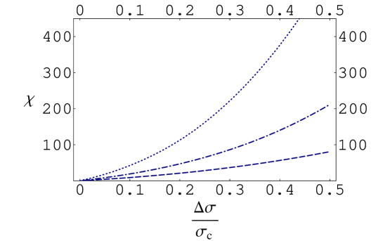
Figure 1: The two-dimensional numerical result for the function $\chi(g/\sqrt{\lambda},\Delta\sigma/\sigma_{c})$ for the values $g/\sqrt{\lambda}=\sqrt{2}$ (dashed), $g/\sqrt{\lambda}=1$ (dot-dashed) and $g/\sqrt{\lambda}=1/\sqrt{2}$ (dotted).

The results show for small $\Delta\sigma\ll mg/\lambda$ a scaling according to $g^{-2}\Delta\sigma$, which we explain below. The numerical coefficient turns out to be

$$S_{\rm E}\approx 158\times\frac{\Delta\sigma}{\sigma_{c}}\frac{1}{g^{2}}.$$ (16)

To ensure this scaling behaviour even for very small values for the coupling constants, we will give an analytical upper bound for the Euclidean action in the following. With above insights, we can proceed with further simplifications of the problem. Sizeable tunneling may only occur when the inflaton $\sigma$ is close to its critical value, cf. Fig. 1. Therefore, we assume

$$\Delta\sigma\ll\sigma_{\rm c}.$$ (17)

In order to obtain a lower bound on the tunneling rate, we impose the instanton to follow a straight trajectory in $(\sigma,\phi)$ space. The exact solution along a curved trajectory has a lower Euclidean action and therefore corresponds to a larger tunneling rate. The trajectory is parameterized by

$$\phi = aw\,,$$

$$\sigma = \Delta\sigma+\frac{m}{g}-\sqrt{1-a^{2}}w\,,$$ (18)

where $a\in[0;1]$ is a free parameter that will be determined by minimizing the action. Along this trajectory, the potential (5) close to the critical point takes the form

$$V=\frac{1}{4}\frac{m^{4}}{\lambda}-a^{2}\sqrt{1-a^{2}}gmw^{3}+a^{2}gm\Delta\sigma w^{2}+O\left(w^{2}\Delta\sigma^{2},\;w^{4}\right)\,.$$ (19)

We now determine the value of the parameter $a$, for which the Euclidean bounce action is minimal. For that purpose, we consider the potential

$$V=-\alpha w^{3}+\beta w^{2}\,.$$ (20)

By rescaling arguments, one obtains that the corresponding action has to scale as

$$S_{\rm E}\sim\frac{\beta}{\alpha^{2}}\sim\frac{\Delta\sigma}{m\,g}\times\frac{1}{a^{2}(1-a^{2})}$$ (21)

and is minimized for $a=1/\sqrt{2}$. This explains the scaling behaviour for small $\Delta\sigma$ observed in (16). The comparison with Eq. (15) yields for the linearized case

$$S_{E} \sim \quad\frac{\Delta\sigma}{\sigma_{c}}\frac{1}{g^{2}}\,,$$ (22)

$$\chi(g/\sqrt{\lambda},\Delta\sigma/\sigma_{c}) \sim \left(\frac{g}{\sqrt{\lambda}}\right)^{-2}\times\frac{\Delta\sigma}{\sigma_{c}}\,.$$ (23)

For the choice $a=1/\sqrt{2}$, neglecting the $w^{4}$ terms in the approximated linearized potential (19) is justified when

$$w\ll\sqrt{32}\sigma_{\rm c}\frac{g^{2}}{\lambda}\,,$$ (24)

and the $w^{2}\Delta\sigma^{2}$ terms are subdominant if

$$\Delta\sigma\ll 2\sigma_{\rm c}\,.$$ (25)

Numerically, we find for the constant of proportionality

$$S_{\rm E}=182\times\frac{\Delta\sigma}{\sigma_{c}}\frac{1}{g^{2}}\,,$$ (26)

where the larger factor of proportionality when compared with (16) is due to the fact that we are restricted to the linear path and therefore miss the minimum of the Euclidean action in the two-dimensional field space. We also note that the point $w_{\rm r}$, from which the field $w$ in the bounce solution is released, scales according to

$$w_{\rm r}=8.2\times\frac{\Delta\sigma}{\sigma_{\rm c}}\frac{m}{g}=8.2\times\Delta\sigma\,.$$ (27)

Notice that a small Euclidean action, $S_{\rm E}\ll 1$, automatically ensures the requirements in Eqs. (24) and (25) and hence the validity of the approximation in Eq. (19), if $g,\lambda<1$.

Finally, when assuming $m$ to be of order of the Grand Unified Scale $10^{16}\,{\rm GeV}$ or less, all scales in the problem are larger than the Hubble rate

$$H=\sqrt{\frac{8\pi V}{3m_{\rm Pl}^{2}}}\,,$$ (28)

where $m_{\rm Pl}=1.22\times 10^{19}\,{\rm GeV}$ denotes the Planck mass, such that gravitational effects can be neglected [10].

3 Bounds on Specific Models

We estimate the relevant values for $\Delta\sigma$ using the standard slow-roll dynamics of the inflaton. When the expectation value of the inflaton, at a certain instant during inflation, takes the value $\sigma=\sigma_{\rm e}$, the number of e-foldings $N_{\rm e}$ that will elapse until inflation ends is calculated as

$$N_{\rm e}=\int\limits_{\sigma_{\rm e}}^{\sigma_{\rm c}}H\,dt=\frac{8\pi}{m_{\rm Pl}^{2}}V\int\limits_{\sigma_{\rm c}}^{\sigma_{\rm e}}\frac{d\sigma}{\partial V/\partial\sigma}\,,$$ (29)

where we have used the slow-roll approximation $3H\partial\sigma/\partial t=-\partial V/\partial\sigma$. One important observational constraint is the amplitude $\sqrt{P_{\cal R}}$ of the power spectrum of scalar perturbations for the scale $k$, that exits the horizon when $\sigma=\sigma_{\rm e}$,

$$\sqrt{P_{\cal R}}=\sqrt{\frac{\pi}{6}}\frac{16}{m_{\rm Pl}^{3}}\frac{V^{3/2}}{\partial V/\partial\sigma}\,\Bigg{|}_{\sigma=\sigma_{\rm e}}\,.$$ (30)

Here, we impose the normalization [11]

$$\sqrt{P_{\cal R}}=4.5\times 10^{-5}$$ (31)

at $k=0.05\,{\rm Mpc^{-1}}$. This scale exits the horizon at

$$N_{\rm e}=50+\frac{1}{3}\log_{10}\frac{T_{\rm R}}{10^{9}\,{\rm GeV}}+\frac{2}{3}\log_{10}\frac{V^{1/4}}{10^{15}\,{\rm GeV}}\,.$$ (32)

Since $k=0.05\,{\rm Mpc^{-1}}$ corresponds to multipole moments around $\ell=700$, the largest angular observable scales have exited the horizon about six to seven e-folds earlier.

A very conservative estimate for $\Delta\sigma$ and therefore the tunneling rate is therefore obtained by setting $N_{\rm e}=60$ and

$$\Delta\sigma=\sigma_{\rm e}-\sigma_{\rm c}\,.$$ (33)

We use this value to compute the Euclidean action (26) and to estimate the tunneling rate (4). The latter is to be compared with the expansion rate during inflation $H$, e.g. the number of non-inflationary bubbles nucleated per expansion time in one horizon is given by $\Gamma/({\cal V}H^{4})$ and should be much less than one. An interesting, but difficult question would be to quantify how much less. Due to the exponentially strong dependence of the tunneling rate on the model parameters, we omit a discussion of this question by the same token on which we do not evaluate the determinants in Eq. (4).

We furthermore remark that it appears very likely that for viable inflationary models, one has to impose that tunneling also does not occur at much lower values of $N_{\rm e}$ than 60. The nucleation of non-inflationary bubbles would lead to very large density perturbations on small scales, which induce the production of primordial black holes [12], which is strongly constrained observationally [13]. We do not discuss this possibility here any further and just explore the conservative bound.

3.1 Blue Model – Quadratically Lifted Flat Direction

In the seminal work [2], hybrid inflation is implemented by a quadratically lifted flat direction, through the effective potential

$$V_{\rm L}(\sigma)=\frac{1}{2}m_{\sigma}^{2}\sigma^{2}\,.$$ (34)

Due to the positive curvature of the potential along the flat direction, the scalar perturbations are predicted to be blue tilted, which is characterized by a scalar spectral index $n_{\rm s}>1$. Using (29) and the basic potential (5), we can solve for

$$\sigma_{\rm e}=\frac{m}{g}\exp\left\{\frac{\lambda}{2\pi}\frac{m_{\rm Pl}^{2}m_{\sigma}^{2}}{m^{4}}N_{\rm e}\right\}\,,$$ (35)

while the amplitude of the power spectrum (30) is given by

$$\sqrt{P_{\cal R}}=\sqrt{\frac{2}{3}\pi}\frac{gm^{5}}{\lambda^{3/2}m_{\rm Pl}^{3}m_{\sigma}^{2}}\,.$$ (36)

The latter two equations can be solved for $m_{\sigma}$ and $\sigma_{\rm e}$ by assuming that the exponent in (35) is small, approximating $\sigma_{\rm e}\approx\sigma_{\rm c}$, and justifying this a posteriori. We find

$$m_{\sigma}^{2}=\frac{g}{\lambda^{3/2}}\sqrt{\frac{2\pi}{3P_{\cal R}}}\frac{m^{5}}{m_{\rm Pl}^{3}}\,,$$ (37)

and

$$\sigma_{\rm e}=\frac{m}{g}\exp\left\{\frac{g}{\sqrt{6\pi\lambda P_{\cal R}}}\frac{m}{m_{\rm Pl}}N_{\rm e}\right\}\,,$$ (38)

such that

$$\Delta\sigma\approx\frac{1}{\sqrt{6\pi\lambda P_{\cal R}}}\frac{m^{2}}{m_{\rm Pl}}N_{\rm e}$$ (39)

Inserting these into (26) and using (31) yields

$$S_{\rm E}=\frac{42}{g\sqrt{\lambda P_{\cal R}}}\frac{m}{m_{\rm Pl}}N_{\rm e}=\frac{9.3\times 10^{5}}{g\sqrt{\lambda}}\frac{m}{m_{\rm Pl}}N_{\rm e}\,.$$ (40)

We now discuss the self-consistency of the above results. For the approximation of the potential $V$ by expression (19) to be valid for the bounce solution, we have to fulfill the relation (24) with $w=w_{\rm r}$. Using (27) and (39) with $N_{\rm e}=60$, we find the bound

$$m\ll 2.2\times 10^{-6}\frac{g}{\sqrt{\lambda}}m_{\rm Pl}\,.$$ (41)

This condition also ensures the validity of the assumption $\Delta\sigma\ll\sigma_{\rm c}$, in particular that the exponent in (38) is much smaller than one.

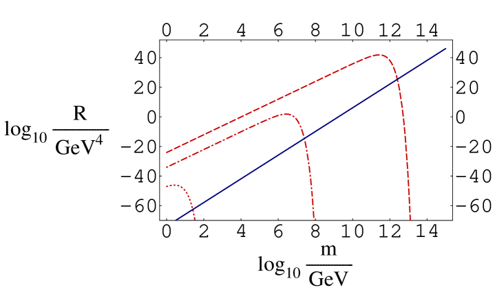
Figure 2: Hubble expansion vs. tunneling decay in the blue model. The plot shows $\log_{10}R$ for $R=H^{4}$ (solid) and $R=\Gamma/{\cal V}$ for $g=0.5$ (dashed), $g=5\times 10^{-6}$ (dot-dashed) and $g=5\times 10^{-12}$ (dotted). We have chosen $\lambda=0.5$.

In order to summarize these results, we present Fig. 2. A reasonable estimate of the tunneling rate is given by

$$\frac{\Gamma}{\cal V}=\frac{S_{\rm E}^{2}}{4\pi^{2}}g^{4}m^{4}{\rm e}^{-S_{\rm E}},$$ (42)

since $gm$ is the smallest dimensionful scale occurring in the approximate potential (19). We compare the decay rate with the Hubble rate (28), since $(\Gamma/{\cal V})/H^{4}$ is the number of bubbles nucleating in one Hubble time within a Hubble volume. Note that for the range of $m$ for the individual graphs of $\Gamma/{\cal V}$ in Fig. 2, the consistency condition (41) is met. The wide range of orders of magnitude covered relativizes the importance of the prefactor of the exponential in the expression for $\Gamma/{\cal V}$, in particular the determinants in Eq. (4). Also the precise bound on the tunneling rate loses importance due to its strong dependence on $m$ after it has reached is maximum. As a conservative requirement, we may impose $(\Gamma/{\cal V})<H^{4}$. A bound which is stronger by a few orders of magnitude might be in order to accord with observation, but has no significant impact on the tunneling bound on $m$.

An important implication to be read off from Fig. (2) is that for the TeV-scale as a special scale of interest, $g$ has to be smaller than at most $10^{-11}$ in order to avoid a fast end of inflation through tunneling, provided $\lambda$ is of order one. Besides by suppressing $g$, we see from Eq. (40), that also small values of $\lambda$ serve to suppress the tunneling rate. Choosing this option however leads to expectation values for $\phi$ after inflation and $\sigma$ during inflation, which are much larger than $m$. If one considers $m$ as a cutoff scale or to be closely related to a cutoff scale of an effective theory, this is undesirable.

As a curiosity, we note that we rule out a particular choice of parameters used as an example in the original work on hybrid inflation [2], $m=1.3\times 10^{11}\,{\rm GeV}$, $g^{2}=\lambda=0.1$. In this case, $\Gamma/{\cal V}=1.3\times 10^{33}\,{\rm GeV}^{4}$, whereas $H^{4}=1.7\times 10^{14}\,{\rm GeV}^{4}$, indicating that $\Gamma/({\cal V}H^{4})=7.6\times 10^{18}$ non-inflationary bubbles are nucleated during one expansion time within a horizon.

3.2 Red Model

Since the WMAP3 data strongly prefers a red-tilted scalar spectral index $n_{\rm s}$, with the best-fit value given by $n_{\rm s}\approx 0.95$ [11], we also study models with a negative curvature along the flat direction. A simple possible realization of these is given by

$$V_{\rm L}=A^{3}\sigma-\frac{1}{2}m_{\sigma}^{2}\sigma^{2}\,.$$ (43)

During inflation, the inflaton takes values in between $\sigma_{\rm c}$ and the maximum of $V_{\rm L}$, which is located at $\sigma=A^{3}/m_{\sigma}^{2}$. This translates into the requirement

$$\frac{m}{g}<\frac{A^{3}}{m_{\sigma}^{2}}\,.$$ (44)

Note that this model has an additional parameter when compared with the quadratically lifted model, which is fixed by imposing the value of the spectral index of the scalar perturbations $n_{\rm s}=0.95$ as an additional constraint. It is calculated through the slow-roll parameter $\eta$ as

$$n_{\rm s}=1+2\eta\,,$$ (45)

where

$$\eta=\frac{m_{\rm Pl}^{2}}{8\pi}\frac{\partial^{2}V/\partial\sigma^{2}}{V}\,.$$ (46)

Imposing the spectral index constraint together with equations (29) and (30), we find the relations

$$m_{\sigma}^{2} = -\eta\frac{2\pi}{\lambda}\frac{m^{4}}{m_{\rm Pl}^{2}}\,,$$ (47)

$$A^{3} = -\frac{2\pi\eta}{g\lambda}\frac{m^{5}}{m_{\rm Pl}^{2}}+\sqrt{\frac{2\pi}{3P_{\cal R}}}\lambda^{-3/2}\frac{m^{6}}{m_{\rm Pl}^{3}}{\rm e}^{-\eta N_{\rm e}}\,,$$ (48)

$$\sigma_{\rm e} = \frac{m}{g}+\frac{1-\exp\{-\eta N_{\rm e}\}}{\eta\sqrt{6\pi\lambda P_{\cal R}}}\frac{m^{2}}{m_{\rm Pl}}\,.$$ (49)

With the numerical result for the Euclidean action (26) and the power spectrum normalization (31), this gives

$$S_{\rm E}=\frac{42}{\eta g\sqrt{\lambda P_{\cal R}}}\left(1-\exp\{-\eta N_{\rm e}\}\right)\frac{m}{m_{\rm Pl}}=\frac{9.3\times 10^{5}}{\eta g\sqrt{\lambda}}\left(1-\exp\{-\eta N_{\rm e}\}\right)\frac{m}{m_{\rm Pl}}\,,$$ (50)

and, when additionally imposing $N_{\rm e}=60$, $\eta=-0.025$,

$$S_{\rm E}=\frac{1.3\times 10^{8}\,m}{g\sqrt{\lambda}m_{\rm Pl}}\,.$$ (51)

The consistency condition (24) with $w=w_{\rm r}$ for our approximation is fulfilled when

$$m\ll 9.7\times 10^{-7}\frac{g}{\sqrt{\lambda}}m_{\rm Pl}\,.$$ (52)

Again, we have found that tunneling is preferred for large couplings $\lambda$ and $g$ and small values for the mass parameter $m$, where the small ratio to the Planck scale is imposed by the small amplitude of density perturbations. Comparison of the Euclidean actions for the blue model (40) and the red (51) with $N_{\rm e}=60$ shows that both differ only by a proportionality factor which is irrelevant with respect to the level of our approximation. The figure for the blue model is therefore almost indistinguishable for the eye when compared to Fig. 2 for the red model, which is why it is omitted here.

We note that for the above models, one should bear in mind that in order to obtain the effective potentials (34) and (43) in the parametric range which allows for tunneling decay, one has to require a more than substantial amount of tuning. For hybrid inflation at the Electroweak scale, this is discussed in [14, 15]. The one-loop correction to the tree-level hybrid potential (5) is given by

$$V_{1-{\rm loop}}=\frac{1}{64\pi^{2}}\left(m^{2}-g^{2}\sigma^{2}\right)^{2}\log\frac{g^{2}\sigma^{2}-m^{2}}{\Lambda^{2}}\,,$$ (53)

where $\Lambda$ is an ultraviolet cutoff. Suppose now, we choose the renormalizable counterterms, which are the terms up to fourth order in $\sigma$, in such a way that for $\sigma=\sigma_{\rm e}$, we have the desired values for $m_{\sigma}$ and $A$, while the cubic and quartic self-couplings cancel to zero. When now expanding the potential around $\sigma_{\rm e}$ down to values of $\sigma\stackrel{{\scriptstyle>}}{{{}_{\sim}}}\sigma_{\rm c}$, the nonrenormalizable fifth order term, which we did not eliminate, induces an additional mass for the field $\sigma$ of order $gm$. This is to be compared with $m_{\sigma}$ as in (37) or (47). In order for the quantum correction to be subdominant, one therefore has to require $g\ll m^{3}/m_{\rm Pl}^{3}$ (blue) or $g\ll m^{2}/m_{\rm Pl}^{2}$ (red), respectively. Comparing with Fig. 2, it is easy to see that tunneling does not play any role within hybrid models which do not require the fine-tuning of nonrenormalizable operators. This reasoning already strongly indicates that the supersymmetric scenarios with radiatively lifted flat directions do not suffer from tunneling either, as we shall see explicitly in the next section, number 3.3.

The above study shows that inflation exit via tunneling is mostly relevant for inflation models with an energy scale below the GUT scale and especially for the intriguing case of models where inflation is connected to electroweak physics and therefore within experimental reach. In fact, a hybrid model has been suggested where the role of the waterfall field $\phi$ is played by the Standard Model Higgs field, such that the field content only needs to be extended by the inflaton singlet $\sigma$ [16, 17]. Since these models apparently also bear the potential for successful baryogenesis, the enormous fine tuning of the potential may be considered worth the price for a minimal field content. However, our analysis shows that for the desired parameters $m/\sqrt{\lambda}=246\,{\rm GeV}$, and the couplings $g,\;\lambda={\cal O}(1)$ in order to allow for strong pre- or reheating, a rapid decay via tunneling is inevitable, such that the electroweak hybrid models are not viable, even if fine tuned.

Another motivation for contemplating low scales of inflation originates from models explaining the hierarchy between the Planck scale and a fundamental unified scale by the presence of large extra dimensions. Inflation then has to take place at energies below the unified scale. Kaloper and Linde [18] point out that hybrid inflation is a possible way to keep the vacuum expectation value of the scalar fields in the effective four-dimensional potential for inflation below the fundamental scale. While they agree with Lyth on the view that when inflation occurs at the Electroweak scale, one faces a severe fine tuning problem, they conclude that models with $M\sim 10^{11}\,{\rm GeV}$, $g^{2}=\lambda=0.1$ fit perfectly in the hybrid scenario, somewhat in contradiction with our estimate $g\ll m^{3}/m_{\rm Pl}^{3}$. Note also our comment on the tunneling rate for this parametric range at the end of section 3.1.

3.3 SUSY Hybrid Inflation

From the general arguments on the irrelevance of the tunneling rate within our approximation for models without fine-tuning of nonrenormalizable operators, it is already clear that tunneling does not play a role in SUSY-hybrid inflation [19, 20]. These models are however of special interest since they rely on rather minimal assumptions and in their simplest version depend only on a single parameter $\kappa$ [21], which can be determined [22] from the latest observational data [11] . They furthermore bear the potential of a successful embedding of the Minimal Supersymmetric Standard Model in an inflationary scenario, possibly linked to a Grand Unified Theory [20, 23, 24, 25]. Due to the importance of these models, we derive here an expression for the Euclidean bounce action $S_{\rm E}$, although it will be large and prohibit tunneling.

$F$-term SUSY hybrid inflation is implemented by the superpotential

$$W=\kappa S\left(G\overline{G}-M^{2}\right)\,,$$ (54)

which leads to the tree-level scalar potential

$$V=\kappa^{2}|G\overline{G}-M^{2}|^{2}+\kappa^{2}|SG|^{2}+\kappa^{2}|S\overline{G}|^{2}\,.$$ (55)

The involved fields are complex, where $S$ is a singlet, $G$ a gauged multiplet of dimension ${\cal N}$ and $\overline{G}$ its conjugate. Vanishing of the $D$-terms relates the vacuum expectation values $\langle G\rangle=\langle\overline{G}\rangle^{*}$.

We choose the phase of $S$ to be zero and identify

$$\sigma=\sqrt{2}{\rm Re}[S]\,.$$ (56)

Likewise, by a unitary gauge choice, such that $\langle{\rm Re}[G^{i}]\rangle=\langle|G|\rangle$, we can set

$$\phi=\sqrt{2}{\rm Re}[G^{i}]\,.$$ (57)

In terms of these fields, the potential (55) reads

$$V=\kappa^{2}M^{4}-\kappa^{2}M^{2}\phi^{2}+\frac{1}{4}\kappa^{2}\phi^{4}+\frac{1}{2}\kappa^{2}\sigma^{2}\phi^{2}\,.$$ (58)

This is a special case of the more general potential (5) with the replacements

$$m^{2} = 2\kappa^{2}M^{2}\,,$$

$$g = \kappa\,,$$

$$\lambda = \kappa^{2}\,.$$ (59)

The lifting of the flat direction is then induced by the Coleman-Weinberg potential [20, 25]

$$V_{\rm L} = \frac{\cal N}{32\pi^{2}}\kappa^{4}\left\{\left(\frac{\sigma^{2}}{2}+M^{2}\right)^{2}\log\left(\kappa^{2}\frac{\frac{1}{2}\sigma^{2}+M^{2}}{\Lambda^{2}}\right)+\left(\frac{\sigma^{2}}{2}-M^{2}\right)^{2}\log\left(\kappa^{2}\frac{\frac{1}{2}\sigma^{2}-M^{2}}{\Lambda^{2}}\right)\right.$$ (60)

$$\left.-\frac{1}{2}\sigma^{4}\log\left(\kappa^{2}\frac{1}{2}\frac{\sigma^{2}}{\Lambda^{2}}\right)\right\}\,.$$

We consider again the situation where $\sigma$ is close to the critical point, such that we can approximate

$$\frac{\partial V_{\rm L}}{\partial\sigma}\approx\sqrt{2}\log 2\frac{\cal N}{8\pi^{2}}\kappa^{4}M^{3}+O(M^{2}\Delta\sigma)\,,$$ (61)

where the critical point is at $\sigma=\sigma_{\rm c}=\sqrt{2}M$ and $\Delta\sigma=\sigma-\sigma_{c}$. Within this approximation, the number of e-folds (29) is

$$N_{\rm e}=\frac{64\pi^{3}}{\sqrt{2}\log 2}\frac{M\Delta\sigma}{\kappa^{2}{\cal N}m_{\rm Pl}^{2}}\,.$$ (62)

Imposing the normalization of the power spectrum (30), we get a relation between $\kappa$ and $M$,

$$M=\kappa^{1/3}\left(\frac{\sqrt{3\,P_{\cal R}}\,{\cal N}\log 2}{\pi^{5/2}}\right)^{1/3}\frac{m_{\rm Pl}}{4}\,,$$ (63)

such that we can derive

$$\Delta\sigma=(\log 2)^{1/3}2^{-3/2}3^{-1/3}\pi^{-4/3}\kappa^{4/3}\left(\sqrt{P_{\cal R}}\right)^{-2/3}M{\cal N}^{1/3}N_{\rm e}\,.$$ (64)

Using (26), we find for the Euclidean tunneling action

$$S_{\rm E}=6.1\left(\kappa\sqrt{P_{\cal R}}\right)^{-2/3}{\cal N}^{1/3}N_{\rm e}=4800\kappa^{-2/3}{\cal N}^{1/3}N_{\rm e}\,.$$ (65)

Tunneling therefore does not occur within $F$-term SUSY-hybrid inflation.

We have also performed a corresponding study for the $D$-term model [26, 27], which is more involved due to the additional parametric dependence on the gauge coupling constant. However, as one can already anticipate from the general arguments about radiative corrections and tunneling given at the end of section 3.2, we find that tunneling is also very suppressed in these scenarios. We therefore omit a detailed presentation of the derivation of this negative result.

4 Conclusions

Imposing the normalization of the scalar perturbation spectrum (30), it is possible to estimate for generic models of hybrid inflation the range of parameters where tunneling dominates over the slow-roll evolution of the inflaton fields. In order to calculate the Euclidean action $S_{\rm E}$, we have assumed that the bounce solution follows a straight trajectory in the field space spanned by the inflaton and the waterfall field. We have numerically obtained the action for a particular set of parameters and then used its scaling properties in order to calculate the tunneling rates in parametric regions of small couplings and small field values, which are difficult to access numerically. This result is expressed in Eq. (26), which we have used to derive constraints on hybrid inflation, arising from the requirement that tunneling should be suppressed. The consistency of our approach is verified by a comparison with the numerically determined results for the bounce action along the curved extremal path in two-dimensional field space.

Our results are best summarized by the formulas (40), (51) and by Fig. 2. Tunneling may play a role for models with a mass below $10^{12}\,{\rm GeV}$, but can effectively be suppressed by small values of the inflaton-waterfall coupling $g$ and the waterfall self coupling $\lambda$, which in turn imply large expectation values of the inflaton field during inflation or the waterfall field after its end.

Provided one does not allow for the fine-tuning of nonrenormalizable operators, tunneling never constitutes a problem. In particular, one cannot derive any tunneling bounds on the parameters of $F$- or $D$-term SUSY models. In contrast, models of electroweak hybrid inflation, which need coupling constants of order one for a sufficient reheating of the Universe but require fine-tuning, are completely ruled out since the inflaton would rapidly decay through bubble nucleation. Leaving alone the issue of stability of the inflaton potential with respect to radiative corrections, tunneling decay prohibits the realization of hybrid inflation when the vacuum energy and all field expectation values are required to be at scales below $10^{12}\,{\rm GeV}$.

References

- [1] See e.g. D. H. Lyth and A. Riotto, “Particle physics models of inflation and the cosmological density perturbation,” Phys. Rept. 314 (1999) 1 [arXiv:hep-ph/9807278].
- [2] A. D. Linde, “Axions in inflationary cosmology,” Phys. Lett. B 259 (1991) 38; A. D. Linde, “Hybrid inflation,” Phys. Rev. D 49 (1994) 748 [arXiv:astro-ph/9307002].
- [3] S. R. Coleman, “The Fate Of The False Vacuum. 1. Semiclassical Theory,” Phys. Rev. D 15 (1977) 2929 [Erratum-ibid. D 16 (1977) 1248].
- [4] C. G. . Callan and S. R. Coleman, “The Fate Of The False Vacuum. 2. First Quantum Corrections,” Phys. Rev. D 16 (1977) 1762.
- [5] K. M. Lee and E. J. Weinberg, “Tunneling Without Barriers,” Nucl. Phys. B 267 (1986) 181.
- [6] A. D. Linde, “Decay Of The False Vacuum At Finite Temperature,” Nucl. Phys. B 216 (1983) 421 [Erratum-ibid. B 223 (1983) 544].
- [7] G. N. Felder, L. Kofman and A. D. Linde, “Tachyonic instability and dynamics of spontaneous symmetry breaking,” Phys. Rev. D 64 (2001) 123517 [arXiv:hep-th/0106179].
- [8] T. Konstandin and S. J. Huber, “Numerical approach to multi dimensional phase transitions,” JCAP 0606 (2006) 021 [arXiv:hep-ph/0603081].
- [9] J. M. Cline, G. D. Moore and G. Servant, “Was the electroweak phase transition preceded by a color broken phase?,” Phys. Rev. D 60 (1999) 105035 [arXiv:hep-ph/9902220].
- [10] S. R. Coleman and F. De Luccia, “Gravitational Effects On And Of Vacuum Decay,” Phys. Rev. D 21 (1980) 3305.
- [11] D. N. Spergel et al., “Wilkinson Microwave Anisotropy Probe (WMAP) three year results: Implications for cosmology,” arXiv:astro-ph/0603449.
- [12] B. J. Carr, “The Primordial Black Hole Mass Spectrum,” Astrophys. J. 201 (1975) 1.
- [13] A. M. Green and A. R. Liddle, “Constraints on the density perturbation spectrum from primordial black holes,” Phys. Rev. D 56 (1997) 6166 [arXiv:astro-ph/9704251].
- [14] D. H. Lyth, “Constraints on TeV-scale hybrid inflation and comments on non-hybrid alternatives,” Phys. Lett. B 466 (1999) 85 [arXiv:hep-ph/9908219].
- [15] E. J. Copeland, D. Lyth, A. Rajantie and M. Trodden, Phys. Rev. D 64 (2001) 043506 [arXiv:hep-ph/0103231].
- [16] J. Garcia-Bellido, D. Y. Grigoriev, A. Kusenko and M. E. Shaposhnikov, “Non-equilibrium electroweak baryogenesis from preheating after Phys. Rev. D 60 (1999) 123504 [arXiv:hep-ph/9902449].
- [17] L. M. Krauss and M. Trodden, “Baryogenesis below the electroweak scale,” Phys. Rev. Lett. 83 (1999) 1502 [arXiv:hep-ph/9902420].
- [18] N. Kaloper and A. D. Linde, “Inflation and large internal dimensions,” Phys. Rev. D 59 (1999) 101303 [arXiv:hep-th/9811141].
- [19] E. J. Copeland, A. R. Liddle, D. H. Lyth, E. D. Stewart and D. Wands, “False vacuum inflation with Einstein gravity,” Phys. Rev. D 49 (1994) 6410 [arXiv:astro-ph/9401011].
- [20] G. R. Dvali, Q. Shafi and R. K. Schaefer, “Large scale structure and supersymmetric inflation without fine tuning,” Phys. Rev. Lett. 73 (1994) 1886 [arXiv:hep-ph/9406319].
- [21] V. N. Senoguz and Q. Shafi, “Testing supersymmetric grand unified models of inflation,” Phys. Lett. B 567 (2003) 79 [arXiv:hep-ph/0305089].
- [22] R. A. Battye, B. Garbrecht and A. Moss, “Constraints on supersymmetric models of hybrid inflation,” JCAP 0609 (2006) 007 [arXiv:astro-ph/0607339].
- [23] B. Kyae and Q. Shafi, “Inflation with realistic supersymmetric SO(10),” Phys. Rev. D 72 (2005) 063515 [arXiv:hep-ph/0504044].
- [24] B. Garbrecht, T. Prokopec and M. G. Schmidt, “SO(10) - GUT coherent baryogenesis,” Nucl. Phys. B 736 (2006) 133 [arXiv:hep-ph/0509190].
- [25] B. Garbrecht and A. Pilaftsis, “F(D)-term hybrid inflation with electroweak-scale lepton number violation,” Phys. Lett. B 636 (2006) 154 [arXiv:hep-ph/0601080]; B. Garbrecht, C. Pallis and A. Pilaftsis, “Anatomy of F(D)-term hybrid inflation,” arXiv:hep-ph/0605264.
- [26] E. Halyo, “Hybrid inflation from supergravity D-terms,” Phys. Lett. B 387 (1996) 43 [arXiv:hep-ph/9606423].
- [27] P. Binetruy and G. R. Dvali, “D-term inflation,” Phys. Lett. B 388 (1996) 241 [arXiv:hep-ph/9606342].