QCD sum rule approach to the new mesons and the $g_{D_{sJ}DK}$ coupling constant

Abstract

We use diquark-antidiquark currents to investigate the masses and partial decay widths of the recently observed mesons $D_{sJ}^{+}(2317)$, $D_{0}^{*0}(2308)$ and $X(3872)$, considered as four-quark states, in a QCD sum rule approach. In particular we investigate the coupling constant $g_{D_{sJ}DK}$. We found that the $g_{D_{sJ}DK}$ obtained in this four-quark scenario is smaller than the coupling constant obtained when $D_{sJ}^{+}(2317)$ is considered as a conventional $c\bar{s}$ state.

I Introduction

The constituent quark model provides a rather successful descrition of the spectrum of the mesons in terms of quark-antiquark bound states, which fit into the suitable multiplets reasonably well. Therefore, it is understandable that the recent observations of the very narrow resonances $D_{sJ}^{+}(2317)$ by BaBar babar , $D_{sJ}^{+}(2460)$ by CLEO cleo , $X(3872)$ by BELLE BELLE , and the very broad scalar meson $D_{0}^{*0}(2308)$ by BELLE belle2 , all of them with masses below quark model predictions, have stimulated a renewed interest in the spectroscopy of open charm and charmonium states. The difficulties to identify the mesons $D_{sJ}^{+}(2317)$ and $D_{sJ}^{+}(2460)$ as $c\bar{s}$ states are rather similar to those appearing in the light scalar mesons below 1 GeV (the isoscalars $\sigma(500),~{}f_{0}(980)$, the isodublet $\kappa(800)$ and the isovector $a_{0}(980)$), that can be interpreted as four-quark states jaffe ; cloto . In the case of $X(3872)$, besides its small mass, the observation, reported by the BELLE collaboration belleE , that the $X$ decays to $J/\psi\,\pi^{+}\pi^{-}\pi^{0}$, with a strength that is compatible to that of the $J/\psi\pi^{+}\pi^{-}$ mode:

$${Br(X\to J/\psi\,\pi^{+}\pi^{-}\pi^{0})\over Br(X\to J/\psi\,\pi^{+}\pi^{-})}=1.0\pm 0.4\pm 0.3\;,$$ (1)

establishes strong isospin violating effects, which can not be explained if the $X(3872)$ is interpreted as a $c\bar{c}$ state.

Due to these facts, these new mesons were considered as good candidates for four-quark states by many authors Swanson . In refs. blmnn ; x3872 the method of QCD sum rules (QCDSR) svz ; rry ; narison was used to study the two-point functions for the mesons $D_{sJ}^{+}(2317)$, $D_{0}^{*0}(2308)$and $X(3872)$ considered as four-quark states in a diquark-antidiquark configuration. The results obtained for their masses are compatible with the experimental values and, therefore, in refs. blmnn ; x3872 the authors concluded that it is possible to reproduce the experimental value of the masses using a four-quark representation for these states.

Concerning their decay widths, the study of the three-point functions related to the decay widths $D_{sJ}^{+}(2317)\to D_{s}^{+}\pi^{0}$, $D_{0}^{*0}\to D^{+}\pi^{-}$ and $X(3872)\to J\psi\pi^{+}\pi^{-}$, using the diquark-antidiquark configuration for $D_{sJ}$, $D_{0}^{*0}$ and $X$, was done in refs. decayds ; decayd0 ; decayx . The results obtained for their partial decay widths are given in Table I, from where we see that the partial decay widths obtained in refs. decayds ; decayd0 , supposing that the mesons $D_{sJ}^{+}(2317)$ and $D_{0}^{*0}$ are four-quark states, are consistent with the experimental upper information for the total decay width.

Table 1: Numerical results for the resonance decay widths

decay	$D_{sJ}^{+}\to D_{s}^{+}\pi^{0}$	$D_{0}^{*0}\to D^{+}\pi^{-}$	$X\to J/\psi\pi^{+}\pi^{-}$
$\Gamma$ (MeV)	$(6\pm 2)\times 10^{-3}$	$120\pm 20$	$50\pm 15$
$\Gamma^{exp}_{tot}$ (MeV)	$<5$	$270$	$<2.3$

However, in the case of the meson $X(3872)$, the partial decay width obtained in ref. decayx is much bigger than the experimental upper limit to the total width.

In ref. decayx some arguments were presented to reduce the value of the $X(3872)$ decay width, by imposing that the initial four-quark state needs to have a non-trivial color structure. In this case, its partial decay width can be reduced to $\Gamma(X\to J/\psi\pi^{+}\pi^{-}))=(0.7\pm 0.2)~{}\nobreak\,\mbox{MeV}$. However, that procedure may appear somewhat unjustified and, therefore, more study is needed until one can arrive at a definitive conclusion about the structure of the meson $X(3872)$.

Concerning the meson $D_{sJ}^{+}(2317)$, although its mass and decay width can be explained in a four-quark scenario, they can also be reproduced in other approaches Swanson , and it is not yet possible to discriminate between the different structures proposed for this state. Therefore, it is important to find experimental observations that could be used to descriminate between the different quark structure of these mesons. As pointed out in ref. polosa , a signal could be obtained by the analysis of certain heavy-ion collision observables. In particular, the meson $D_{sJ}^{+}(2317)$ can be produced in reactions induced by photons on kaon targets in a nuclear medium formed in a heavy-ion collision. Therefore, if the coupling constant, $g_{D_{sJ}DK}$, is found to be very different depending on the structure for $D_{sJ}^{+}(2317)$, then the photo-production of $D_{sJ}^{+}(2317)$ can be used as a signal to descriminate its structure.

II The $g_{D_{sJ}DK}$ coupling constant

The coupling, $g_{D_{sJ}DK}$, supposing that the meson $D_{sJ}^{+}(2317)$ is a conventional $c\bar{s}$ state, was evaluated in ref. ww . They got:

$$g_{D_{sJ}DK}=(9.2\pm 0.5)~{}\nobreak\,\mbox{GeV}$$ (2)

Here, we extend the calculation done in refs. decayds ; decayd0 to study the hadronic vertex $D_{sJ}DK$. The QCDSR calculation for the vertex, $D_{sJ}DK$, centers around the three-point function given by

$$T_{\mu}(p,p^{\prime},q)=\int d^{4}xd^{4}y~{}e^{ip^{\prime}.x}~{}e^{iq.y}\langle 0|T[j_{D}(x)j_{5\mu}(y)j^{\dagger}_{D_{sJ}}(0)]|0\rangle,$$ (3)

where $j_{D_{sJ}}$ is the interpolating field for the scalar $D_{sJ}$ meson blmnn :

$$j_{D_{sJ}}={\epsilon_{abc}\epsilon_{dec}\over\sqrt{2}}\left[(u_{a}^{T}C\gamma_{5}c_{b})(\bar{u}_{d}\gamma_{5}C\bar{s}_{e}^{T})+u\leftrightarrow d\right],$$ (4)

where $a,~{}b,~{}c,~{}...$ are colour indices and $C$ is the charge conjugation matrix. In Eq. (3), $p=p^{\prime}+q$ and the interpolating fields for the kaon and for the $D$ mesons are given by:

$$j_{5\mu}=\bar{s}_{a}\gamma_{\mu}\gamma_{5}q_{a},\,\;\;\;j_{D}=i\bar{q}_{a}\gamma_{5}c_{a},$$ (5)

where $q$ stands for the light quark $u$ or $d$.

The calculation of the phenomenological side proceeds by inserting intermediate states for $D$, $K$ and $D_{sJ}$, and by using the definitions: $\langle 0|j_{5\mu}|K(q)\rangle=iq_{\mu}F_{K}$, $\langle 0|j_{D}|D(p^{\prime})\rangle={m_{D}^{2}f_{D}\over m_{c}}$, $\langle 0|j_{D_{sJ}}(p)\rangle=\lambda$. We obtain the following relation:

$$T_{\mu}^{phen}(p,p^{\prime},q) = {\lambda m_{D}^{2}f_{D}F_{K}~{}g_{D_{sJ}DK}/m_{c}\over(p^{2}-m_{D_{sJ}}^{2})({p^{\prime}}^{2}-m_{D}^{2})(q^{2}-m_{K}^{2})}~{}~{}q_{\mu}$$ (6)

$$+ \mbox{continuum contribution}\;,$$

where the coupling constant, $g_{D_{sJ}DK}$, is defined by the on-mass-shell matrix element: $\langle DK|D_{sJ}\rangle=g_{D_{sJ}DK}$. The continuum contribution in Eq.(6) contains the contributions of all possible excited states.

In the case of the light scalar mesons, considered as diquark-antidiquark states, the study of their vertices functions using the QCD sum rule approach at the pion pole narison ; rry ; nari2 , was done in ref.sca . It was shown that the decay widths determined from the QCD sum rule calculation are consistent with existing experimental data. Here, we follow ref. bracco and work at the kaon pole. The main reason for working at the kaon pole is that one does not have to deal with the complications associated with the extrapolation of the form factor dosch . The kaon pole method consists in neglecting the kaon mass in the denominator of Eq. (6) and working at $q^{2}=0$. In the OPE side one singles out the leading terms in the operator product expansion of Eq.(3) that match the $1/q^{2}$ term. Since we are working at $q^{2}=0$, we take the limit $p^{2}={p^{\prime}}^{2}$ and we apply a single Borel transformation to $p^{2},{p^{\prime}}^{2}\rightarrow M^{2}$. In the phenomenological side, in the structure $q_{\mu}$ we get:

$$T^{phen}(M^{2}) = {\lambda m_{D}^{2}f_{D}F_{K}~{}g_{D_{sJ}DK}\over m_{c}(m_{D_{sJ}}^{2}-m_{D}^{2})}\left(e^{-m_{D}^{2}/M^{2}}-e^{-m_{D_{sJ}}^{2}/M^{2}}\right)$$ (7)

$$+ A~{}e^{-s_{0}/M^{2}}+\int_{u_{0}}^{\infty}\rho_{cc}(u)~{}e^{-u/M^{2}}du,$$

where $A$ and $\rho_{cc}(u)$ stands for the pole-continuum transitions and pure continuum contributions, with $s_{0}$ and $u_{0}$ being the continuum thresholds for $D_{sJ}$ and $D$ respectively decayds ; decayd0 . For simplicity, one assumes that the pure continuum contribution to the spectral density, $\rho_{cc}(u)$, is given by the result obtained in the OPE side. Therefore, one uses the ansatz: $\rho_{cc}(u)=\rho_{OPE}(u)$. In Eq.(7), $A$ is a parameter which, together with $g_{D_{sJ}DK}$, has to be determined by the sum rule.

In the OPE side we single out the leading terms proportional to $q_{\mu}/q^{2}$. Transferring the pure continuum contribution to the OPE side, the sum rule for the coupling constant, up to dimension 7, is given by:

$$C~{}\left(e^{-m_{D}^{2}/M^{2}}-e^{-m_{D_{sJ}}^{2}/M^{2}}\right)+A~{}e^{-s_{0}/M^{2}}=$$ (8)

$$= {1\over\sqrt{2}}\left[{\langle\bar{q}q\rangle+\langle\bar{s}s\rangle\over 2^{4}\pi^{2}}\int_{m_{c}^{2}}^{u_{0}}du~{}e^{-u/M^{2}}u\left(1-{m_{c}^{2}\over u}\right)^{2}\right.$$

$$+ {m_{c}m_{s}\langle\bar{s}s\rangle\over 2^{5}\pi^{2}}\int_{m_{c}^{2}}^{u_{0}}du~{}e^{-u/M^{2}}\left(1-{m_{c}^{2}\over u}\right)^{2}+{m_{s}\langle\bar{q}q\rangle\langle\bar{s}s\rangle\over 12}e^{-m_{c}^{2}/M^{2}}$$

$$- \left.{m_{c}\langle\bar{q}q\rangle(\langle\bar{q}q\rangle+\langle\bar{s}s\rangle)\over 3}e^{-m_{c}^{2}/M^{2}}\right],$$

with

$$C={\lambda m_{D}^{2}f_{D}F_{K}\over m_{c}(m_{D_{sJ}}^{2}-m_{D}^{2})}~{}g_{D_{sJ}DK}.$$ (9)

III Results and conclusions

In the numerical analysis of the sum rules, the values used for the meson masses, quark masses and condensates are: $m_{D_{sJ}}=2.317~{}\nobreak\,\mbox{GeV}$, $m_{D}=1.87~{}\nobreak\,\mbox{GeV}$, $m_{c}=1.2\,\nobreak\,\mbox{GeV}$, $m_{s}=.13\,\nobreak\,\mbox{GeV}$ $\langle\bar{q}q\rangle=\,-(0.23)^{3}\,\nobreak\,\mbox{GeV}^{3}$, $\langle\bar{s}s\rangle=0.8\langle\bar{q}q\rangle$. For the meson decay constants we use $F_{K}=160~{}\nobreak\,\mbox{MeV}$ and $f_{D}=0.22~{}\nobreak\,\mbox{GeV}$ cleo2 . We use $u_{0}=6~{}\nobreak\,\mbox{GeV}^{2}$ and for the current meson coupling, $\lambda$, we are going to use the result obtained from the two-point function in ref. blmnn . Considering $2.6\leq\sqrt{s_{0}}\leq 2.8~{}\nobreak\,\mbox{GeV}$ we get $\lambda=(2.9\pm 0.3)\times 10^{-3}~{}\nobreak\,\mbox{GeV}^{5}$.

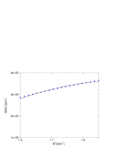
Figure 1: Dots: the RHS of Eq.(8), as a function of the Borel mass. The solid line gives the fit of the QCDSR results through the LHS of Eq.(8).

In Fig. 1 we show, through the dots, the right-hand side (RHS) of Eq.(8) as a function of the Borel mass. To determine $g_{D_{sJ}DK}$ we fit the QCDSR results with the analytical expression in the left-hand side (LHS) of Eq.(8):

$$C\left(e^{-m_{D_{s}}^{2}/M^{2}}-e^{-m_{D_{sJ}}^{2}/M^{2}}\right)+A~{}e^{-s_{0}/M^{2}},$$ (10)

Using $\sqrt{s_{0}}=2.7\nobreak\,\mbox{GeV}$ we get: $C=4.53\times 10^{-4}~{}\nobreak\,\mbox{GeV}^{7}$ and $A=-4.68\times 10^{-4}~{}\nobreak\,\mbox{GeV}^{7}$. Using the definition of $C$ in Eq.(9) and $\lambda=2.9\times 10^{-3}~{}\nobreak\,\mbox{GeV}^{5}$ (the value obtained for $\sqrt{s_{0}}=2.7\nobreak\,\mbox{GeV}$) we get $g_{D_{sJ}DK}=2.8~{}\nobreak\,\mbox{GeV}$. Allowing $s_{0}$ to vary in the interval $2.6\leq\sqrt{s_{0}}\leq 2.8~{}\nobreak\,\mbox{GeV}$, the corresponding variation obtained for the coupling constant is

$$2.5~{}\nobreak\,\mbox{GeV}\leq g_{D_{sJ}DK}\leq 3.8~{}\nobreak\,\mbox{GeV}.$$ (11)

Fixing $\sqrt{s_{0}}=2.7\nobreak\,\mbox{GeV}$ and varying the quark condensate, the charm quark and the strange quark masses in the intervals: $-(0.24)^{3}\leq\langle\bar{q}q\rangle\leq-(0.22)^{3}\,\nobreak\,\mbox{GeV}^{3}$, $1.1\leq m_{c}\leq 1.3\nobreak\,\mbox{GeV}$ and $0.11\leq m_{s}\leq 0.15\nobreak\,\mbox{GeV}$, we get results for the coupling constant still between the lower and upper limits given above. it is important to mention that the agreement between the RHS and LHS of the sum rule in Fig.1 is not so good, in this case, as it was in the case of the couplings $g_{D_{sJ}D_{s}\pi}$ and $g_{D_{0}^{*0}D\pi}$ evaluated in refs. decayds ; decayd0 . One possible reason for that is the fact that the kaon mass is much bigger than the pion mass. Therefore, neglecting the kaon mass in Eq. (6) is not an approximation as good as it is in the case of the sum rule in the pion pole.

We have presented a QCD sum rule study of the vertex function associated with the hadronic vertex $D_{sJ}DK$, where the $D_{sJ}(2317)$ meson was considered as diquark-antidiquark state. Comparing the results in Eqs. (11) and (2) we see that when the meson $D_{sJ}(2317)$ is considered as a conventional $c\bar{s}$ state one gets a $g_{D_{sJ}DK}$ coupling constant much bigger than when $D_{sJ}(2317)$ is considered a four-quark state. This result can be usefull to experimentally investigate the quark structure of the meson $D_{sJ}(2317)$ through its photon production in a nuclear medium.

Acknowledgements

This work has been supported by CNPq and FAPESP.

References

- (1) BABAR Coll., B. Auber et al., Phys. Rev. Lett. 90, 242001 (2003); Phys. Rev. D69, 031101 (2004).
- (2) CLEO Coll., D. Besson et al., Phys. Rev. D68, 032002 (2003).
- (3) BELLE Coll., S.-L. Choi et al., Phys. Rev. Lett. 91, 262001 (2003).
- (4) BELLE Coll., K. Abe et al., Phys. Rev. D69, 112002 (2004).
- (5) R.L. Jaffe, Phys. Rev. D15, 267, 281 (1977); D17, 1444 (1978).
- (6) for a review see F.E. Close and N.A. Törnqvist, J. Phys. G28, R249 (2002).
- (7) K. Abe et al. [Belle Collaboration], hep-ex/0505037, hep-ex/0505038.
- (8) for a review see E. S. Swanson, Phys. Rept. 429, 243 (2006).
- (9) M.E. Bracco et al., Phys. Lett. B624, 217 (2005).
- (10) R. Matheus, S. Narison, M. Nielsen and J.-M. Richard, hep-ph/0608297.
- (11) M.A. Shifman, A.I. and Vainshtein and V.I. Zakharov, Nucl. Phys., B147, 385 (1979).
- (12) L.J. Reinders, H. Rubinstein and S. Yazaky, Phys. Rep. 127, 1 (1985).
- (13) S. Narison, QCD spectral sum rules , World Sci. Lect. Notes Phys. 26, 1; QCD as a theory of hadrons, Cambridge Monogr. Part. Phys. Nucl. Phys. Cosmol. 17, 1-778 (2002) [hep-h/0205006].
- (14) M. Nielsen, Phys. Lett. B634, 35 (2006).
- (15) M. Nielsen, F.S. Navarra and M.E. Bracco hep-ph/0609184.
- (16) F.S. Navarra and M. Nielsen, Phys. Lett. B639, 272 (2006).
- (17) A.D. Polosa, hep-ph/0609137.
- (18) Z.G. Wang, S.L. Wan, Phys. Rev. D73, 094020 (2006).
- (19) S. Narison, Phys. Lett. B175, 88 (1986); S. Narison and R. Tarrach, Phys. Lett. B125, 217 (1983).
- (20) T.V. Brito et al., Phys. Lett. B608, 69 (2005).
- (21) M.E. Bracco, F.S. Navarra, M. Nielsen, Phys. Lett. B454, 346 (1999).
- (22) R.S. Marques de Carvalho et al., Phys. Rev. D60, 034009 (1999).
- (23) CLEO Coll., M. Artuso et al., Phys. Rev. Lett. 95, 251801 (2005).