Model study of the sign problem in the mean-field approximation

Abstract

We argue the sign problem of the fermion determinant at finite density. It is unavoidable not only in Monte-Carlo simulations on the lattice but in the mean-field approximation as well. A simple model deriving from Quantum Chromodynamics (QCD) in the double limit of large quark mass and large quark chemical potential exemplifies how the sign problem arises in the Polyakov loop dynamics at finite temperature and density. In the color SU(2) case our mean-field estimate is in excellent agreement with the lattice simulation. We combine the mean-field approximation with a simple phase reweighting technique to circumvent the complex action encountered in the color SU(3) case. We also investigate the mean-field free energy, from the saddle-point of which we can estimate the expectation value of the Polyakov loop.

I Introduction

Quantum Chromodynamics (QCD) exhibits various states of matter depending on the environment review : A strongly coupled quark-gluon plasma (sQGP) has been discovered at the Relativistic Heavy Icon Collider (RHIC) sQGP and various color superconductors presumably exist in the cores of the compact stellar object CSC . These are widely-known extreme states of equilibrated QCD matter at high temperature and at high (baryon or quark) density, respectively. The study on sQGP properties at high temperature has been led by the Monte-Carlo simulation of QCD on the lattice lattice . The lattice QCD results provide us with fundamental information such as the phase transition temperature $T_{\text{c}}$ Tc , equation of state Aoki:2005vt , susceptibility Bernard:2004je , mesonic correlation above $T_{\text{c}}$ charmonium , etc.

In contrast, at finite density, the lattice technique is not quite successful so far; it is hindered by the notorious problem that the fermion determinant in the presence of nonzero quark chemical potential $\mu_{q}$ is not positive semidefinite (i.e. not nonnegative). This problem is commonly refereed to as the fermion sign problem review:signproblem . The Monte-Carlo simulation based on importance sampling requires positive semidefinite probability for each gauge configuration. In the presence of $\mu_{q}\neq 0$, however, the probability is no longer a well-defined quantity due to a negative fermion determinant arising. There have been several techniques proposed to handle the sign problem, e.g. the reweighting method reweighting , the Taylor expansion method Taylor , the analytical continuation from an imaginary chemical potential imaginary . Although these proposals have achieved partial successes when $\mu_{q}/T$ is small, no prescription applicable at high density has been established yet.

This work is aimed to point out that the sign problem is relevant even in the mean-field treatment of gauge fields. One can intuitively understand it in the following way; in the mean-field approximation the partition function is estimated from the most dominant contribution of particular configurations that have the largest probability or the smallest free energy. When the probability for each gauge configuration is ill-defined due to the sign problem, hence, the mean-field free energy may well be problematic.

In the present work we shall focus on a specific manifestation of the sign problem appearing in the simplest model at finite temperature and density. Because QCD is a highly nontrivial theory, applicability of the mean-field approximation is quite limited. We choose a finite temperature model because the mean-field description presumably works well to sketch the hot QCD phase transition. The Polyakov loop plays an essential role as an order parameter there polyakov_loop . The dynamics of the Polyakov loop was closely examined some years ago both in the lattice simulation polyakov_lattice and in the mean-field approximation weiss ; strong . Recently, in addition, the Polyakov loop dynamics near $T_{\text{c}}$ is specifically paid attention pl_model . There is also an interesting observation that the entanglement between the chiral and Polyakov loop dynamics turns out to be indispensable to understand the nature of the QCD phase transitions go_model ; hatta ; Fukushima:2003fw .

We have already known several indications from the mean-field studies about the Polyakov loop behavior at $\mu_{q}\neq 0$. In the best of our knowledge, the effective potential of the Polyakov loop at finite temperature and density was first derived in Ref. KorthalsAltes:1999cp in perturbative QCD in the one-loop order. (See also Ref. Weiss:1987mp for the potential with an imaginary chemical potential.) It is obvious from Eq. (5) in Ref. KorthalsAltes:1999cp that the Polyakov loop variable is augmented to a complex valued variable when $\mu_{q}\neq 0$, and thus the effective potential turns complex. It is quite nontrivial how to derive meaningful information from such a complex effective potential; the expectation value of the Polyakov loop cannot be fixed directly by a minimum of the complex effective potential. The same problem occurs also in the chiral effective models with the Polyakov loop coupling which was first formulated by one of the present authors in Ref. Fukushima:2003fw and has been investigated extensively fnjl ; Ratti:2005jh , though the sign problem has been almost overlooked. Here, we would refer to a closely related work, Ref. Dumitru:2005ng , in which the authors mentioned on the sign problem in a matrix model of the Polyakov loop. It should be noted that the mean-field free energy as seen in Refs. Ratti:2005jh ; Dumitru:2005ng is not complex unlike the effective potential in Ref. KorthalsAltes:1999cp so that one can determine the expectation value of the Polyakov loop without ambiguity. We will go into details of this issue later. Our findings are all consistent with what has been foreseen in Ref. Dumitru:2005ng .

The concept of this work lies not in solving the sign problem but in observing the sign problem in a manageable way, so to speak, in a clean environment. We also demonstrate that a technique which we call the phase reweighting method works fine as a practical prescription in the similar but not the same spirit as in the finite density lattice simulation. We will employ the dense-heavy model obtained from QCD in the double limit of large quark mass and large quark chemical potential Blum:1995cb (see also discussions in Ref. Bender:1991gn ). The reasons we adopt the dense-heavy model are as follows: First, the fermion determinant is exactly calculable as a function of the gauge field. Second, neither the chiral condensate nor the diquark condensate is involved in the dynamics owing to large quark mass. Third, lattice data is available from Ref. Blum:1995cb . From these three reasons the dense-heavy model is considered to be an appropriate implement for our purpose to scrutinize the sign problem within the mean-field approximation.

This paper is organized as follows. In Sec. II we make a brief overview on the sign problem. We formulate the model in Sec. III.1 and the mean-field approximation in Sec. III.2. Then, in Sec. III.3, we examine the color SU(2) case first which is free from the sign problem in order to make sure if the mean-field approximation is reasonable. We next proceed to the SU(3) calculation. In Sec. III.4 we explain the phase reweighting method to circumvent the SU(3) complex fermion determinant and then discuss the validity of our method by viewing the mean-filed effective potential in Sec. III.5. Section IV is devoted to the summary.

II Sign Problem

Here are general discussions on the sign problem of the fermion determinant at finite density. Readers who are already familiar with it can skip to the model study starting from Sec. III. We will later demonstrate how the dense-heavy model concretely embodies the general features mentioned in this section.

The fermion determinant in Euclidean space-time with a quark mass $m_{q}$ and a quark chemical potential $\mu_{q}$ takes the form of

$$\det\mathcal{M}(\mu_{q})\equiv\det\bigl{[}\gamma_{\mu}D^{\mu}+\gamma_{4}\mu_{q}+m_{q}\bigr{]}\,,$$ (1)

where $D^{\mu}\equiv\partial^{\mu}-igA^{\mu}$ is the covariant derivative. It is a well-known argument that $\det\mathcal{M}(\mu_{q})=\det\gamma_{5}\mathcal{M}(\mu_{q})\gamma_{5}=\{\det\mathcal{M}(-\mu_{q})\}^{\ast}$ and thus the fermion determinant is real in the zero density ($\mu_{q}=0$) case. Alternatively, we can explicitly look into the eigenvalue spectrum of the Dirac operator to confirm that the determinant is positive semidefinite as follows: For $\mu_{q}=0$, when $\psi_{n}$ is an eigenstate of $\gamma_{\mu}D^{\mu}$, the eigenvalue $\lambda_{n}$ is pure imaginary because $\gamma_{\mu}D^{\mu}$ is anti-Hermitian where $\gamma_{\mu}$’s are Hermitian in our convention. Since the mass term is simply proportional to unity, $\psi_{n}$ is also an eigenstate of $\gamma_{\mu}D^{\mu}+m_{q}$ with the eigenvalue $\lambda_{n}+m_{q}$. One can show that $\gamma_{5}\psi_{n}$ is an eigenstate of $\gamma_{\mu}D^{\mu}+m_{q}$ having the eigenvalue $-\lambda_{n}+m_{q}=(\lambda_{n}+m_{q})^{\ast}$ from the property $\gamma_{5}\gamma_{\mu}D^{\mu}\gamma_{5}=-\gamma_{\mu}D^{\mu}$. Therefore, the determinant consists of a pair of $\lambda_{n}+m_{q}$ and $(\lambda_{n}+m_{q})^{\ast}$ which makes the whole determinant real and nonnegative as $|\lambda_{n}+m_{q}|^{2}\geq 0$.

In the presence of the chemical potential term the fermion determinant is not necessarily positive semidefinite. When $\psi_{n}$ is an eigenstate of $\gamma_{\mu}D^{\mu}+\gamma_{4}\mu_{q}$ with the eigenvalue $\lambda_{n}$, in the same was as above, one can show that $\gamma_{5}\psi_{n}$ is also an eigenstate of $\gamma_{\mu}D^{\mu}+\gamma_{4}\mu_{q}$ with the eigenvalue $-\lambda_{n}$ which is not $\lambda_{n}^{\ast}$ because $\gamma_{\mu}D^{\mu}+\gamma_{4}\mu_{q}$ is no longer anti-Hermitian. It is apparent from this explanation that, if $\mu_{q}$ is pure imaginary imaginary , $\gamma_{\mu}D^{\mu}+\gamma_{4}\mu_{q}$ is anti-Hermitian so that the fermion determinant turns nonnegative.

If a considered theory has degenerate fermions associated with an internal symmetry under the transformation $T$ and the chemical potential $\mu_{q}$ is replaced by a matrix $\boldsymbol{\mu}$ in internal space transforming like

$$T^{-1}\,\boldsymbol{\mu}\,T=-\boldsymbol{\mu}\;,$$ (2)

then $\det\mathcal{M}(\boldsymbol{\mu})=\{\det\mathcal{M}(\boldsymbol{\mu})\}^{\ast}$, so that the determinant becomes real.

A well-known realization of this comes from the isospin degrees of freedom in flavor ($u$,$d$) space. The isospin chemical potential $\mu\propto\tau_{3}$ and $T=i\tau_{2}$ (or $T=\tau_{1}$) certainly satisfies Eq. (2) where $\tau$’s are the Pauli matrices in ($u$,$d$) space Son:2000xc .

Another realization is the color SU(2) case su2 that is relevant to our model study as we will argue later. The $C$-transformation changes the quark chemical potential $\mu_{q}$ as in Eq. (2). In general cases, however, the $C$-transformation does not give an escape from the sign problem because it also swaps color and anticolor. That is,

$$C^{-1}\gamma_{5}\,\gamma_{\mu}D^{\mu}\,\gamma_{5}C=\bigl{[}\gamma_{\mu}\bigl{(}\partial^{\mu}-ig(A^{\mu})^{C}\bigr{)}\bigr{]}^{\ast}$$ (3)

with $(A^{\mu})^{C}\equiv-(A^{\mu})^{\ast}$. Special for $N_{\text{c}}=2$ is that anticolor is not distinguishable from color since two doublets can make a singlet. Actually $\sigma_{2}(A^{\mu})^{C}\sigma_{2}=A^{\mu}$ where $\sigma$’s are the Pauli matrices in color space. Therefore the SU(2) case is free from the sign problem.

We should note that the fermion determinant being complex is not necessarily harmful on its own. Rather, it is important whether the real or imaginary part of the fermion determinant is positive semidefinite or not. Even though the determinant evaluated for a certain $A^{\mu}$ is a complex number, the functional integral over $A^{\mu}$ amounts to a real value for physical observables. It is understood in view of the relation,

$$\begin{split}&\det\bigl{[}\gamma_{\mu}\bigl{(}\partial^{\mu}-ig(A^{\mu})^{C}\bigr{)}+\gamma_{4}\mu_{q}+m_{q}\bigr{]}\\ =&\Bigl{\{}\det\bigl{[}\gamma_{\mu}D^{\mu}+\gamma_{4}\mu_{q}+m_{q}\bigr{]}\Bigr{\}}^{\ast}\,.\end{split}$$ (4)

We see clearly that the real (imaginary) part of the determinant is $C$-even ($C$-odd). For a $C$-even ($C$-odd) observable, thus, the imaginary (real) part of the determinant vanishes after integration over $A^{\mu}$. Accordingly the genuine problem stems from that the real or imaginary part of the determinant may change its sign depending on the configuration $A^{\mu}$.

III Model Study

We will analyze a simple model to see the sign problem occurring in the mean-field level. As a practice to study the model, we will make the mean-field approximation in the SU(2) case for which we do not have to face the sign problem. We will then observe the sign problem in the SU(3) calculation and attempt the phase reweighting method to deal with the complex phase of the fermion determinant.

III.1 Dense-Heavy Model

We will closely analyze a lattice model with dense heavy quarks Blum:1995cb . Let us consider QCD in the limit of $\mu_{q}\to\infty$ so that we can drop antiquarks. We shall simultaneously take another limit of $m_{q}\to\infty$ which renders all quarks static. Under such limits we can evaluate the staggered fermion determinant exactly to reach the fermion action,

$$e^{-S_{\text{f}}[L]}\equiv \det\bigl{[}\gamma_{\mu}D^{\mu}+\gamma_{4}\mu_{q}+m_{q}\bigr{]}$$

$$\to \bigl{[}\det(1+\epsilon L)\bigr{]}^{N_{\text{f}}/4}\,,$$ (5)

where $N_{\text{f}}$ is the number of flavors. Not to go into subtlety of the flavor counting inherent to the staggered formalism, which is not of our interest, we set $N_{\text{f}}=4$ throughout this paper.

We take those two limits in a way characterized by the parameter $\epsilon$ ranging from zero to infinity;

$$\epsilon\equiv\Bigl{(}\frac{e^{\mu_{q}a}}{2m_{q}a}\Bigr{)}^{N_{\tau}}\,.$$ (6)

We will often call this model parameter as the “density” parameter because $\epsilon$ has strong correlation to the quark number density as seen in Fig. 1 for the SU(2) case and Fig. 9 for the SU(3) case. Here $N_{\tau}$ is the number of the lattice sites in the temporal direction, that is, the inverse temperature $1/T$ is given by $N_{\tau}a$ with the lattice spacing $a$. In this model quarks are allowed to propagate only in the positive temporal direction. Each time a quark with mass $m_{q}$ travels by one temporal lattice, it picks up the hopping parameter $1/(2m_{q}a)$ and the gauge invariant chemical potential factor $e^{\mu_{q}a}$ Hasenfratz:1984em . After $N_{\tau}$ hops, a quark winds around the temporal circle. It results in the weight $\epsilon$ for the quark excitation represented by the Polyakov loop $L$ in the fundamental representation,

$$L(\vec{x}) \equiv\prod_{x_{4}=a}^{N_{\tau}a}U_{4}(\vec{x},x_{4})$$

$$\equiv\mathcal{P}\exp\biggl{[}\,ig\!\int_{0}^{1/T}\!\!dx_{4}\,A_{4}(\vec{x},x_{4})\biggr{]}\,.$$ (7)

The first line is the expression of the Polyakov loop in terms of link variables on the lattice and second is in the continuum. It does not matter whichever expression we use since the SU($N_{\text{c}}$) matrix $L$ plays the role of the dynamical variable in our model and we will not return to its definition.

The calculation of the determinant in color space is explicitly doable. After all we have the fermion action,

$$e^{-S_{\text{f}}[L]}=\prod_{\vec{x}}\bigl{[}1+\epsilon^{2}+2\epsilon\ell\bigr{]}$$ (8)

in the color $N_{\text{c}}=2$ case (and $N_{\text{f}}=4$ is implicit as we already noted) and

$$e^{-S_{\text{f}}[L]}=\prod_{\vec{x}}\bigl{[}1+\epsilon^{3}+3\epsilon\ell+3\epsilon^{2}\ell^{\ast}\bigr{]}$$ (9)

in the color $N_{\text{c}}=3$ case. In the above expressions we employed the traced Polyakov loop defined as

$$\ell=\frac{1}{N_{\text{c}}}\text{tr}L,$$ (10)

where tr is taken in fundamental color space. We remark that the $C$-transformation changes $\ell$ to $\ell^{\ast}$ and vice versa, where $\ell$ is real for $N_{\text{c}}=2$ and generally complex for $N_{\text{c}}\neq 2$.

It is obvious that the $N_{\text{c}}=2$ determinant (8) is real and positive semidefinite for any $\epsilon$ because $1+\epsilon^{2}+2\epsilon\ell\geq(1-|\epsilon|)^{2}\geq 0$, while the $N_{\text{c}}=3$ expression (9) suffers the sign problem for nonzero $\epsilon$; the determinant can be complex except when either $\epsilon=0$ (zero density), $\epsilon=1$ (half-filling), or $\epsilon\to\infty$ (full-filling). We can intuitively understand why the SU(3) determinant becomes real for $\epsilon=1$. One-quark excitation represented by $\ell$ and two-quark excitation that is equivalent to one-antiquark excitation represented by $\ell^{\ast}$ occur with the common weight $\epsilon=\epsilon^{2}=1$ because of half-filling (see $n=0.5$ at $\epsilon=1$ in Figs. 1 and 9). Therefore, in effect, the system has equality in number of quarks and (effective) antiquarks just like in the zero density case. It is not an escape from the sign problem, however. In the $N_{\text{c}}=3$ case $\ell+\ell^{\ast}$ can take a value ranging from $-1$ to $2$, and thus the determinant at $\epsilon=1$, i.e. $\det(1+L)\propto 2+3(\ell+\ell^{\ast})$ is real but can be negative for $-1<\ell+\ell^{\ast}<-2/3$.

We note here one more important feature of the model. The fermion determinant is invariant under the duality transformation Blum:1995cb ,

$$\epsilon\>\leftrightarrow\>1/\epsilon\quad\text{and}\quad\ell\>\leftrightarrow\>\ell^{\ast}\,,$$ (11)

by which it is sufficient for us to investigate the model in the region $\epsilon\in[0,1]$ and the outer region $\epsilon\in(1,\infty]$ can be deduced by means of the duality.

Regarding the gluodynamics, we assume the nearest neighbor interaction between the Polyakov loops,

$$S_{\text{g}}[L]=-N_{\text{c}}^{2}J\sum_{\text{n.n.}}\ell(\vec{x})\,\ell^{\ast}(\vec{y}).$$ (12)

This action looks pretty simple and still reproduces the fundamental nature of the phase transition in the pure gluonic sector; the action (12) leads to a second-order phase transition for the SU(2) case and a first-order phase transition for the SU(3) case Kogut:1981ez , which is in agreement with the lattice QCD simulation and the theoretical expectation from center symmetry polyakov_loop .

One can interpret $J$ as a model parameter specifying the “temperature” of the system. In the strong coupling expansion, in fact, $J$ is related to $T$ through $J=\exp[-\sigma a/T]$ where $\sigma$ is the string tension. In this work we shall leave $J$ as a model parameter as it is, for we do not want to introduce any further modeling into our analyses. In other words, our aim is to form a model not to imitate QCD itself but to mimic the QCD sign problem.

The effective action that defines our model is eventually given by

$$S[L]=S_{\text{g}}[L]+S_{\text{f}}[L]$$ (13)

with the “density” parameter $\epsilon$ contained in $S_{\text{f}}[L]$ and the “temperature” parameter $J$ in $S_{\text{g}}[L]$.

III.2 Mean Field Approximation

In the finite-temperature field theory the free energy is evaluated in the functional integral form like the effective action as

$$e^{-f\cdot V/T}=\int\!\mathcal{D}L\,e^{-S[L]}\;.$$ (14)

We make use of the mean-field technique to approximate the free energy. Our ansatz for the mean-field action is go_model

$$S_{\text{mf}}[L]\equiv-\frac{x}{2}\sum_{\vec{x}}\bigl{[}\ell(\vec{x})+\ell^{\ast}(\vec{x})\bigr{]}\;.$$ (15)

In case of pure gluonic theories, the mean-field $x$ is simply proportional to the Polyakov loop expectation value; $x=12N_{\text{c}}^{2}J\langle\ell\rangle$. In the presence of fermionic contributions, however, there is no simple relation between them. Besides, $\langle\ell\rangle$ and $\langle\ell^{\ast}\rangle$ in the SU(3) case have different dependence on $\mu_{q}$. One might think that there should be two independent mean-fields to deal with differing $\langle\ell\rangle$ and $\langle\ell^{\ast}\rangle$. This idea has much to do with the sign problem actually, and we will come back to this point later.

Then the mean-field free energy can be estimated as

$$f_{\text{mf}}(x)\cdot V/T=\langle S[L]-S_{\text{mf}}[L]\rangle_{\text{mf}}-\ln\!\int\mathcal{D}L\,e^{-S_{\text{mf}}[L]},$$ (16)

where the average $\langle\cdots\rangle_{\text{mf}}$ is taken by the mean-field action $S_{\text{mf}}[L]$. Roughly speaking, the first part corresponds to the internal energy and the logarithmic part is the entropy. We fix $x$ so as to minimize $f_{\text{mf}}(x)$. Once $S_{\text{mf}}[L]$ is known with $x$ determined, the expectation value of any observable $\mathcal{O}[L]$ as a function of the Polyakov loop can be estimated by the group integration over $L$ with the mean-field action $S_{\text{mf}}[L]$;

$$\langle\mathcal{O}[L]\rangle\simeq\langle\mathcal{O}[L]\rangle_{\text{mf}}\equiv\frac{\displaystyle\int\!dL\,\mathcal{O}[L]\,e^{-S_{\text{mf}}[L]}}{\displaystyle\int\!dL\,e^{-S_{\text{mf}}[L]}}\,.$$ (17)

For instance, the quark number density per color degrees of freedom is available by calculating

$$n\equiv-\frac{1}{N_{\text{c}}}\cdot\frac{\partial f}{\partial\mu_{q}}\simeq\frac{\epsilon}{N_{\text{c}}V}\biggl{\langle}\frac{dS_{\text{f}}}{d\epsilon}\biggr{\rangle}_{\text{mf}}\,.$$ (18)

One can calculate the Polyakov loop susceptibility $\chi$ in the same way which reflects information of the deconfinement phase transition. If one directly uses $\mathcal{O}[L]=\ell^{2}$ in the mean-field approximation, however, nothing becomes singular at the critical point unless the fluctuation of $\ell$ is taken into account. Equivalently one can estimate the susceptibility from the inverse curvature of the effective potential because the one-loop fluctuation leads to the trace of propagator for $\langle\ell^{2}\rangle$, that is, the inverse screening mass. Since $\langle\ell\rangle$ and $\langle\ell^{\ast}\rangle$ are uniquely determined given $x$ is fixed by the free energy (16), one can regard $f_{\text{mf}}(x)$ as a function of $\langle\ell\rangle$ or $\langle\ell^{\ast}\rangle$. The Polyakov loop susceptibility is then

$$\biggl{(}\frac{\partial^{2}f_{\text{mf}}}{\partial\langle\ell\rangle^{2}}\biggr{)}^{-1}=\biggl{(}\frac{\partial\langle\ell\rangle}{\partial x}\biggr{)}^{2}\biggl{(}\frac{\partial^{2}f_{\text{mf}}}{\partial x^{2}}\biggr{)}^{-1}\,,$$ (19)

where we used $\partial f_{\text{mf}}/\partial x=0$. Of course, the susceptibility defined in terms of $\ell^{\ast}$ is available with $(\partial\langle\ell\rangle/\partial x)^{2}$ replaced by $(\partial\langle\ell^{\ast}\rangle/\partial x)^{2}$. The difference thus lies only in the nonsingular coefficient we are not interested in. For our purpose it is rather convenient to focus on the singular part alone discarding the difference of $\langle\ell\rangle$ and $\langle\ell^{\ast}\rangle$. Hence, we define the susceptibility as

$$\chi\equiv\biggl{(}\frac{\partial^{2}f_{\text{mf}}}{\partial^{2}x}\biggr{)}^{-1}$$ (20)

for presenting our numerical results.

Now that we finish explaining our approximations and computational procedures, let us step forward to the model analysis.

III.3 SU(2) Results

We consider the model in the color SU(2) case first, as we mentioned, to see how the mean-field approximation works apart from the sign problem.

Figure 1: Correlation between the density parameter $\epsilon$ and the quark number density per lattice site (i.e. density in the unit of the lattice spacing) divided by $N_{\text{c}}=2$. It is obvious from the figure that $\epsilon=0$ is the zero-density ($n=0$) state and $\epsilon=1$ is the half-filling ($n=0.5$) one.

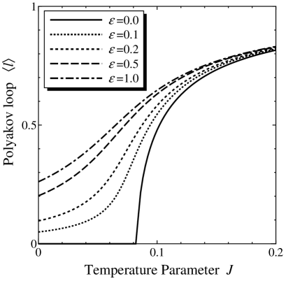
Figure 2: SU(2) (traced) Polyakov loop $\langle\ell\rangle$ as a function of the coupling $J$ at various density parameters; $\epsilon=$0 (solid), 0.1 (dotted), 0.2 (short-dashed), 0.5 (dashed), and 1.0 (dotted-dashed). The second-order phase transition at $\epsilon=0$ occurs at $J_{\text{c}}\simeq 0.083$. The transitional behavior is gradually smeared by the center symmetry breaking terms in the fermion determinant as $\epsilon$ grows larger.

Figure 3: SU(2) Polyakov loop $\langle\ell\rangle$ as a function of the density parameter $\epsilon$ at various temperature parameters; $J$=0 (solid), 0.05 (short-dashed), 0.1 (dashed), and 0.2 (dotted-dashed). The Polyakov loop becomes insensitive to $\epsilon$ as $J$ goes larger, which is consistent with Fig. 2 in which the results at various $\epsilon$ converge at large $J$.

Figure 1 shows the results for the quark number density $n$ as a function of the density parameter $\epsilon$ using Eq. (18). For $\epsilon>1$ the duality relation $n(\epsilon)=1-n(1/\epsilon)$ enables us to deduce the number density. We can immediately confirm from this plot and the duality relation that the density parameter specifies the quark number density uniquely which monotonously approaches unity as $\epsilon\to\infty$. It should be noted that the half-filling $n=0.5$ realizes at $\epsilon=1$ and there is no $J$ dependence at all then.

Let us look at the phase transition seen in the Polyakov loop behavior with increasing $J$. The deconfinement phase transition in the SU(2) pure gluonic theory is known to be second-order belonging to the same universality class as the Ising model polyakov_loop ; polyakov_lattice ; Engels:1989fz . In our model at $\epsilon=0$ we have a continuous transition at $J=J_{\text{c}}\simeq 0.083$ as indicated by the solid curve in Fig. 2. The presence of dynamical quarks acts on the Polyakov loop variable as an external field breaking center symmetry. In fact, the results at nonzero $\epsilon$ in Fig. 2 are not of transition but of crossover.

We plot the density dependence of the Polyakov loop behavior in Fig. 3. The density effects generally tend to make the Polyakov loop larger, and eventually, the Polyakov loop becomes insensitive to the density in the large $J$ (i.e. high temperature) region. It is because both the temperature and the density break center symmetry spontaneously and explicitly, respectively, having the Polyakov loop saturated. Therefore, the $J$ dependence is less for larger $\epsilon$ and the $\epsilon$ dependence is less for larger $J$.

Figure 4: Comparison to the number density measured on the lattice at $4/g^{2}=2.0$ (circle) and $4/g^{2}=1.5$ (square) taken from Fig. 1 in Ref. Blum:1995cb .

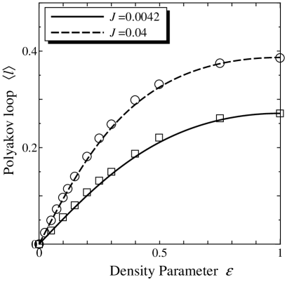
Figure 5: Comparison to the SU(2) Polyakov loop measured on the lattice at $4/g^{2}=2.0$ (circle) and $4/g^{2}=1.5$ (square) taken from Fig. 2 in Ref. Blum:1995cb .

Our mean-field outputs are to be compared with the lattice simulation in Ref. Blum:1995cb ; our Figs. 1 and 3 correspond to Figs. 1 and 2 presented in Ref. Blum:1995cb , respectively. We cannot expect a quantitative coincidence because our ansatz for the pure gluonic action $S_{\text{g}}[L]$ is only a crude approximation of QCD and besides we neglect the renormalization of the Polyakov loop in the mean-field treatment. Nevertheless, the agreement turns out to be surprisingly good beyond our expectation if we treat the model parameter $J$ as a fitting parameter incorporating the undetermined effect of the Polyakov loop renormalization, which is implied by the ansatz (12). In such a way, we can fix $J=0.0042$ and $J=0.04$ to reproduce the SU(2) Polyakov loop only at $\epsilon=1$ for $4/g^{2}=2.0$ and $4/g^{2}=1.5$, respectively. We would emphasize that we did not use the data of the Polyakov loop at $\epsilon\neq 1$ and not the data of the number density at all. Nevertheless, as clearly seen from the comparisons in Figs. 4 and 5, our numerical results fit all of the lattice data pretty well. We can conclude from this observation that the main QCD corrections to our ansatz (12) could be absorbed into the renormalization of the coupling alone. We are now confident that the mean-field treatment is a fairly acceptable approximation for this type of problem.

Figure 6: Susceptibility relevant to the SU(2) Polyakov loop $\ell$ as a function of $J$ at various density parameters; $\epsilon=$0.0 (solid), 0.1 (short-dashed), 0.2 (dashed), and 1.0 (dotted-dashed). The $\epsilon=0$ result has a divergence at $J=J_{\text{c}}$ characteristic to the second-order phase transition.

Finally let us check that the susceptibility (20) diverges at $\epsilon=0$ and $J=J_{\text{c}}$. Figure 6 shows the susceptibility as a function of $J$ at various $\epsilon$. In the plot $\chi$ becomes greater with increasing $J$ because we did not include $\partial\langle\ell\rangle/\partial x$ in our definition of $\chi$ in Eq. (20). It is intriguing to remark that the $\epsilon=0.1$ result is not really critical in view of $\chi$, while the crossover at $\epsilon=0.1$ in Fig. 2 looks rather close to a phase transition. Actually $\chi$ is a more informative quantity to judge how critical the crossover is in fact.

In summary of the SU(2) Polyakov loop dynamics at finite temperature and density, we shall depict a three-dimensional plot of $\langle\ell\rangle$ in Fig. 7 as a function of the “temperature” $J$ and the “density” $\epsilon$. We immediately see general tendency that $\langle\ell\rangle$ grows up with increasing $J$ and $\epsilon$.

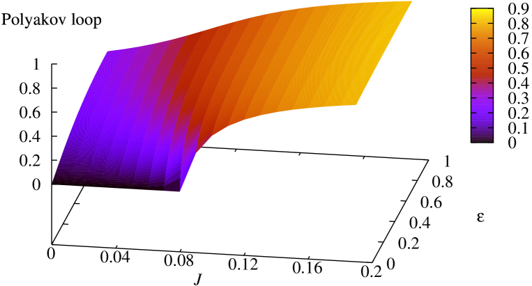
Figure 7: Three-dimensional plot of the fundamental Polyakov loop in the SU(2) case as a function of the temperature parameter $J$ and the density parameter $\epsilon$.

Figure 8: Dependence of the SU(2) adjoint Polyakov loop $\langle\ell_{\text{adj}}\rangle$ on the temperature parameter $J$ at various density parameters; $\epsilon$=0.0 (solid), 0.1 (dotted), 0.2 (short-dashed), 0.5 (dashed), and 1.0 (dotted-dashed).

Before closing this subsection we will comment a bit on the adjoint Polyakov loop whose definition is

$$\ell_{\text{adj}}\equiv\frac{1}{N_{\text{c}}^{2}-1}\text{tr}L^{\text{adj}}=\frac{1}{N_{\text{c}}^{2}-1}\Bigl{(}N_{\text{c}}^{2}|\ell|^{2}-1\Bigr{)}\;.$$ (21)

The adjoint Polyakov loop is no longer an order parameter because the adjoint representation is not faithful by the center of the gauge group. This quantity has been closely argued in Ref. Dumitru:2003hp and there still remain subtleties. Not in the SU(2) but in the SU(3) case, it has been found that $\langle\ell_{\text{adj}}\rangle$ takes an infinitesimally small value in the confined phase. One possible explanation would be that the group integration over $L$ is important in the center symmetric regime where nonperturbative phenomena like color confinement are relevant (see also Ref. Lenz:1998qk ). As a matter of fact, the SU($N_{\text{c}}$) group integration over $\ell_{\text{adj}}$ turns out to be zero, if we are allowed to disregard the dynamics. Even with the dynamics taken into account within the mean-field approximation, as shown in Fig. 8, the argument should hold so $\langle\ell_{\text{adj}}\rangle\simeq 0$ in the low temperature side. However, the adjoint Polyakov loop behavior in our study should be understood only up to a qualitative level. It is pointed out in Ref. Dumitru:2003hp that the renormalization for $\ell_{\text{adj}}$ is significant, which is not considered in our present treatment.

III.4 SU(3) case

In case of $N_{\text{c}}=3$ we have to tackle the sign problem. We are not capable of solving QCD exactly like the lattice simulation, so one might think that within the framework of approximations one is allowed to impose the mean-field ansatz (15) to get some results anyhow. The free energy after the integration over $L$ could be real in terms of $x$. It seems to work at least as a rough estimate that is worth trying first.

The serious flaw in such a simple strategy is that $\langle\ell\rangle=\langle\ell^{\ast}\rangle$ is inevitably concluded. It is, however, contradict to the lattice results Taylor and the model analyses Dumitru:2005ng where $\langle\ell\rangle\neq\langle\ell^{\ast}\rangle$ has been observed at finite density. If the mean-field ansatz (15) is extended to having two variables $x$ and $y$ in order to take account of the difference between $\langle\ell\rangle$ and $\langle\ell^{\ast}\rangle$, the price to pay is that the mean-field free energy is not convex. We will revisit this issue latter. In any case, though the appearance might be unalike, the difficulty of the sign problem is conserved even in the mean-field approximation unless the difference $\langle\ell\rangle\neq\langle\ell^{\ast}\rangle$ is neglected.

In our work we shall elucidate that the “phase reweighting method” is one way to resolve these difficulties. We should, however, note that the reweighting method in the present context is one approximation scheme unlike in the lattice simulation. That is, the reweighting method is expected to be precise if the number of configurations is infinitely large, and thus the lattice simulation with infinite number of configurations generated could provide us with the exact answer in principle, while the mean-field approximation picking up only the most dominant configuration cannot.

III.4.1 Method

The point of the method is that we decompose the fermion determinant into one part that gives the positive semidefinite probability and the other part that is regarded as the observable whose average is taken by configurations.

The complex fermion determinant consists of the $C$-even magnitude and the $C$-odd phase. Accordingly, the fermion action can be rewritten as

$$S_{\text{f}}[L]=S_{\text{f}}^{\text{mag}}[L]+i\Theta[L]\,,$$ (22)

where

$$S_{\text{f}}^{\text{mag}}[L] =-\sum_{\vec{x}}\ln\bigl{|}1+\epsilon^{3}+3\epsilon\ell+3\epsilon^{2}\ell^{\ast}\bigr{|}\,,$$ (23)

$$\Theta[L] =-\sum_{\vec{x}}\arg\bigl{(}1+\epsilon^{3}+3\epsilon\ell+3\epsilon^{2}\ell^{\ast}\bigr{)}\,.$$ (24)

With these definitions we approximate the expectation value of $\mathcal{O}[L]$ by the one obtained as follows;

$$\langle\mathcal{O}[L]\rangle\simeq\frac{\displaystyle\bigl{\langle}\mathcal{O}[L]\,e^{-i\Theta[L]}\bigr{\rangle}_{\text{mf}}}{\displaystyle\bigl{\langle}e^{-i\Theta[L]}\bigr{\rangle}_{\text{mf}}}\;.$$ (25)

Here $S_{\text{mf}}[L]$ or $x$ is fixed from the free energy with the action $S_{\text{g}}[L]+S_{\text{f}}^{\text{mag}}[L]$, so that $x$ encompasses the information of $S_{\text{f}}^{\text{mag}}[L]$ implicitly. This scheme is the same as what has been adopted in the lattice simulation in Ref. Blum:1995cb .

Here we would draw attention to a related work; in Ref. deForcrand:1999cy the correlation between $\text{Im}\ell$ and $\Theta[L]$ was investigated in the lattice simulation, which is apparent in our case from the expression (24).

III.4.2 Results

Figure 9: Correlation between the density parameter $\epsilon$ and the quark number density $n$ per lattice site divided by $N_{\text{c}}=3$. The gross feature is similar to Fig. 1; $\epsilon=0$ is the zero density state ($n=0$) and $\epsilon=1$ is the half-filling state ($n=0.5$) in this SU(3) case as well as in the SU(2) case.

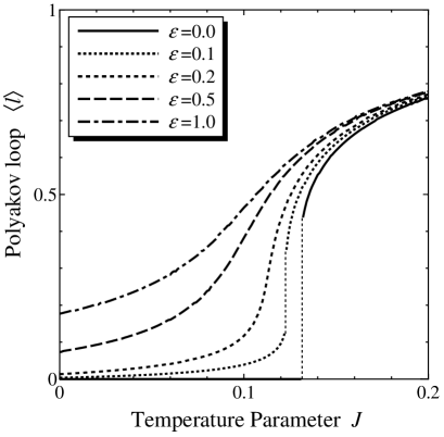
Figure 10: SU(3) (traced) Polyakov loop $\langle\ell\rangle$ as a function of the temperature parameter $J$ at various density parameters; $\epsilon=$0 (solid), 0.1 (dotted), 0.2 (short-dashed), 0.5 (dashed), and 1.0 (dotted-dashed). The first-order phase transition at $\epsilon=0$ and $\epsilon=0.1$ occurs at $J_{\text{c}}=0.132$ and $J_{\text{c}}=0.123$, respectively.

Let us start with checking the monotonous correlation between $\epsilon$ and $n$ as in the SU(2) case. This allows us to regard increase (or decrease) in the density parameter $\epsilon$ as increase (or decrease) in the quark number density $n$. The positive correlation is obvious from the results we show in Fig. 9. The “temperature” or $J$ dependence is slightly greater than the SU(2) results. We can give a possible account for this as follows; in the confined phase at small $J$, the quark number density is suppressed as compared with high $J$ results. This suppression comes from the group integration that forces the thermally excited particles to be not quarks but (nearly) color-singlet baryons consisting of $N_{\text{c}}$ quarks go_model ; Oleszczuk:1992yg . In general larger $N_{\text{c}}$ leads to stronger suppression by heavier excitation quanta. Therefore, the stronger $J$ dependence presented in Fig. 9 originates from the stronger suppression at small $J$. The suppression is physically interpreted as effective tendency toward confinement Fukushima:2003fw .

Figure 10 is the Polyakov loop as a function of $J$ corresponding to the SU(2) result in Fig. 2 and to be compared qualitatively with the lattice result of Fig. 7 in Ref. Blum:1995cb . We find a first-order phase transition for $\epsilon=0$ at $J=J_{\text{c}}=0.132$ and for $\epsilon=0.1$ at $J=J_{\text{c}}=0.123$. The effect of nonzero $\epsilon$ smears the transitional behavior and the phase transition eventually ceases to be of first-order at a certain $\epsilon$. The end-point of the first-order phase boundary is a second-order critical point called the critical end-point, which is of much interest in attempts to clarify the QCD phase diagram CEP ; Asakawa:1989bq . We have crossover at larger $\epsilon$. The global picture is well consistent with what has been already clarified in the Potts system as a toy model of finite temperature and density QCD Alford:2001ug ; Kim:2005ck .

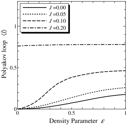
Figure 11: SU(3) Polyakov loop $\langle\ell\rangle$ as a function the density parameter $\epsilon$ at various temperature parameters; $J$=0 (solid), 0.05 (dotted), 0.10 (short-dashed), 0.13 (dashed), and 0.2 (dotted-dashed). The gross feature is similar to the SU(2) case in Fig. 3.

We plot the “density” dependence of the SU(3) Polyakov loop in Fig. 11 which is the SU(3) counterpart of Fig. 3. The SU(2) and SU(3) results are qualitatively similar except for that the Polyakov loop is suppressed at small $J$ and $\epsilon$ just as we found in the quark number density. It would be interesting if we could compare our results with the lattice data, but unfortunately, the SU(3) data as a function of $\epsilon$ is not available from Ref. Blum:1995cb . We cannot argue the $J$ (or $6/g^{2}$) dependence because it involves unknown renormalization effects.

Figure 12: Difference of the SU(3) Polyakov loops $\langle\ell\rangle$ and $\langle\ell^{\ast}\rangle$ as a function of the temperature parameter $J$ at various density parameters; $\epsilon=$0 (solid) which is zero entirely, 0.1 (dotted), 0.2 (short-dashed), and 0.5 (dashed).

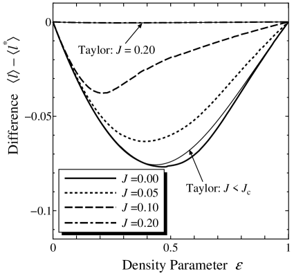
Figure 13: Difference of the SU(3) Polyakov loops $\langle\ell\rangle$ and $\langle\ell^{\ast}\rangle$ as a function of the density parameter $\epsilon$ at various temperature parameters; $J=$0 (solid), 0.05 (short-dashed), 0.1 (dashed), and 0.2 (dotted-dashed). The thin curves represent the results from the Taylor expansion method in the confine phase at $J<J_{\text{c}}$ and in the deconfined phase at $J=0.20>J_{\text{c}}$ which is almost overlaid on the result from the phase reweighting.

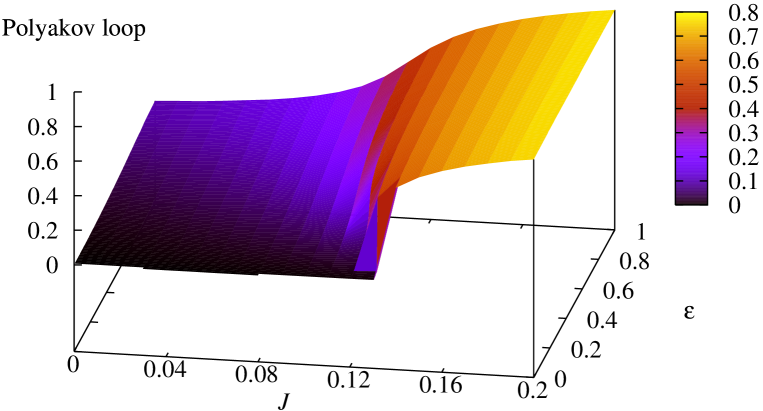
Figure 14: Three-dimensional plot of the fundamental Polyakov loop in the SU(3) case as a function of the temperature parameter $J$ and the density parameter $\epsilon$.

In the phase reweighting calculation we can see how $\langle\ell\rangle$ and $\langle\ell^{\ast}\rangle$ become distinct at $\mu_{q}\neq 0$. The observable $\ell-\ell^{\ast}$ is $C$-odd and so the imaginary part of the fermion determinant is responsible for a nonvanishing difference. When $\epsilon$ is small in the fermionic determinant (9) the imaginary part comes from $\text{Im}\,\epsilon\ell\propto\epsilon(\ell-\ell^{\ast})$. Consequently the expectation value of the difference is proportional to $\epsilon\langle(\text{Im}\,\ell)^{2}\rangle_{0}$ where $\langle\cdots\rangle_{0}$ is taken at zero density Dumitru:2005ng . In Fig. 12 we present our numerical results for the difference $\langle\ell\rangle-\langle\ell^{\ast}\rangle$ as a function of $J$. The difference is trivially zero at $\epsilon=0$ and $\epsilon=1$ where the fermion determinant is real. As long as the density parameter stays smaller than $\epsilon\sim 0.5$, a larger density parameter $\epsilon$ leads to a bigger difference. For example, we find the difference at $\epsilon=0.5$ as large as $\langle\ell\rangle-\langle\ell^{\ast}\rangle=-0.076$ which is comparable to $\langle\ell\rangle=0.073$.

One can intuitively understand why $\langle\ell^{\ast}\rangle$ is greater than $\langle\ell\rangle$ at nonzero $\mu_{q}$, which agrees with what has been observed in the lattice simulation Taylor . It is because, as discussed also in Ref. Taylor , the presence of quarks at finite density enhances the screening effect for antiquarks so that the antiquark excitation costs less energy.

The dense-heavy model, or $e^{-S_{\text{f}}}$, originally takes a form of power series in $\epsilon$ as seen in the expression (9). We have thus performed the Taylor expansion also to estimate the Polyakov loop difference. The expectation value of the coefficient of the $\epsilon$ series is calculated at zero density $\epsilon=0$. In this static model the fermionic contribution is just vanishing at $\epsilon=0$, and so the Taylor expansion method gives rise to the identical output for any $J<J_{\text{c}}$ in the confined phase where $x$ remains zero. In the deconfined phase $J>J_{\text{c}}$ the $J$ dependence is brought in by nonzero $x$. Figure 13 shows the difference $\langle\ell\rangle-\langle\ell^{\ast}\rangle$ as a function of $\epsilon$ at various $J$ with the Taylor expansion results in the confined and deconfined phase. We can see excellent agreement between two methods from the comparison at $J=0.00$ and $J=0.20$. However, the Taylor expansion cannot reproduce the results at $0<J<J_{\text{c}}$ at all. The lesson from our model study is that the Taylor expansion in terms of density breaks down in the presence of the first-order phase transition with respect to temperature. Still, in the deconfined phase at high temperature, the expansion is validated. We do not think that this finding is trivial in our model. In the realistic QCD lattice simulation with $2+1$ flavors, the zero density result is most likely crossover, and thus the Taylor expansion method should be reliable at all temperatures.

As we showed in the previous subsection, we shall present the three-dimensional plot of the SU(3) Polyakov loop as a function of the temperature parameter $J$ and the density parameter $\epsilon$ in Fig. 14. The figure is qualitatively consistent with the lattice result shown in Fig. 5 in Ref. Blum:1995cb .

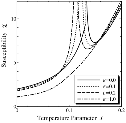
Figure 15: Susceptibility relevant to the SU(3) Polyakov loop $\ell$ as a function of $J$ at various density parameters; $\epsilon=0.0$ (solid), 0.1 (short-dashed), 0.2 (dashed), and 1.0 (dotted-dashed).

Figure 16: SU(3) adjoint Polyakov loop $\langle\ell_{\text{adj}}\rangle$ as a function of the temperature parameter $J$ at various density parameters; $\epsilon$=0.0 (solid), 0.1 (dotted), 0.2 (short-dashed), 0.5 (dashed), and 1.0 (dotted-dashed).

We shall turn to the susceptibility $\chi$ to examine the phase transition more closely. Because the phase transition at small $\epsilon$ is of first-order, $\chi$ jumps discontinuously at $J=J_{\text{c}}$ as seen in Fig. 15. The susceptibility $\chi$ grows as the model parameters approach the critical end-point where the second-order phase transition takes place. Figure 15 implies that the zero density ($\epsilon=0$) result is significantly affected by the critical end-point which should be located nearby at small $\epsilon$. In view of Figs. 6 and 15 the critical region in the SU(3) case is wider than the SU(2) case.

Let us comment on the adjoint Polyakov loop here again. As we mentioned in discussions on the SU(2) results, the adjoint Polyakov loop should require proper renormalization beyond the mean-field treatment. We show the adjoint Polyakov loop result in Fig. 16 just because we can do that. The first-order phase transition is located at the same point; $J=J_{\text{c}}\simeq 0.132$, of course. The group integration over $L$ suppresses $\langle\ell_{\text{adj}}\rangle$ at low $J$ even for large $\epsilon$, which makes the crossover in Fig. 16 look shaper than in case of the fundamental Polyakov loop in Fig. 10.

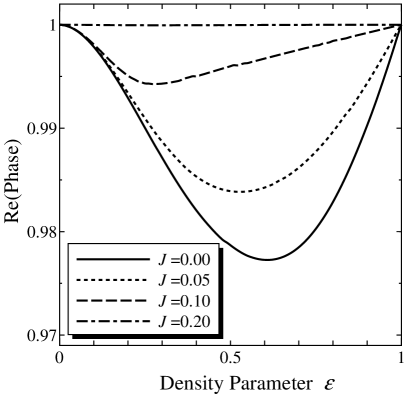
Figure 17: Phase of the fermion determinant $\text{Re}\langle e^{-i\theta}\rangle$ per lattice site as a function of the density parameter $\epsilon$ at various temperature parameters; $J=$0 (solid), 0.05 (short-dashed), 0.10 (dashed), and 0.20 (dotted-dashed).

Finally we present the results for the expectation value of the phase factor of the fermionic determinant, $e^{-i\Theta}$. We plot $\text{Re}\langle e^{-i\theta}\rangle$ as a function of $\epsilon$ in Fig. 17, where $\theta$ is the phase at each lattice site; $\theta\equiv-\arg(1+\epsilon^{3}+3\epsilon\ell+3\epsilon^{2}\ell^{\ast})$ (i.e. $\Theta=\sum_{\vec{x}}\theta$.) Comparing it with Fig. 9 in Ref. Blum:1995cb , we can surely check that our results qualitatively reproduce the lattice data. For more quantitative arguments, let us put the volume $6^{3}=216$ of the lattice simulation in Ref. Blum:1995cb into our results. The expected phase factor $\langle e^{-i\Theta}\rangle$ can be, as a rough estimate, approximated as $(\langle e^{-i\theta}\rangle)^{216}$. For instance, our $J=0$ result has a minimum at $\epsilon=0.61$ where $\langle e^{-i\theta}\rangle\simeq 0.977$, and we get $0.977^{216}=0.0066$. The minimum value in Fig. 9 in Ref. Blum:1995cb is read as of order $0.01$, which is not quite far from our estimate viewed on the logarithmic plot.

III.5 Mean-Field Free Energy

Here we will pursue another strategy to deal with the difference between $\langle\ell\rangle$ and $\langle\ell^{\ast}\rangle$ as a double-check. It is possible to extend the mean-field ansatz as

$$S_{\text{mf}}[L]=-\frac{x}{2}\sum_{\vec{x}}\bigl{[}\ell(\vec{x})\!+\!\ell^{\ast}(\vec{x})\bigr{]}-\frac{y}{2}\sum_{\vec{x}}\bigl{[}\ell(\vec{x})\!-\!\ell^{\ast}(\vec{x})\bigr{]}\,,$$ (26)

and then we can compute the mean-field free energy from Eq. (16) as a function of $x$ and $y$. After the integration over $L$, the free energy $f_{\text{mf}}(x,y)$ is a real function of real variables $x$ and $y$. We can thus fix the mean-fields by

$$\frac{\partial f_{\text{mf}}}{\partial x}\biggr{|}_{(x,y)=(x_{0},y_{0})}=\frac{\partial f_{\text{mf}}}{\partial y}\biggr{|}_{(x,y)=(x_{0},y_{0})}=0\,.$$ (27)

Nonzero $y_{0}$ appears in the presence of nonzero $\mu_{q}$. It turns out that around $(x_{0},y_{0})$ the free energy $f_{\text{mf}}(x,y)$ has a minimum in the $x$ direction, while it has a maximum in the $y$ direction. That is, the solution to Eq. (27) is a saddle-point of $f_{\text{mf}}(x,y)$, which is consistent with Ref. Dumitru:2005ng . The instability with respect to $y$ should be a remnant of the sign problem  We here point out that this instability also exists in the zero density limit; $f_{\text{mf}}(x,y)$ has a saddle-point at $y=0$ even at zero density. It should be instructive to take a closer look at how the saddle-point arises even at zero density. If we expand the free energy in terms of $\langle\ell\rangle$ and $\langle\ell^{\ast}\rangle$, the leading term dependent on $\langle\ell\rangle$ and $\langle\ell^{\ast}\rangle$ is quadratic $\sim\langle\ell\rangle\langle\ell^{\ast}\rangle$ as explicitly seen in a simple estimate in Ref. Ratti:2005jh . This form of the free energy implies an instability inducing $\langle\ell\rangle\neq\langle\ell^{\ast}\rangle$ because it can written as $\langle\ell\rangle\langle\ell^{\ast}\rangle\propto(\langle\ell\rangle\!+\!\langle\ell^{\ast}\rangle)^{2}-(\langle\ell\rangle\!-\!\langle\ell^{\ast}\rangle)^{2}$.

The situation is somewhat analogous to thermodynamics in the finite density NJL-model calculation. If the free energy $f$ is calculated as a function of the renormalized chemical potential $\mu_{q}$ Asakawa:1989bq , then the value of $\mu_{q}$ is fixed by the condition $\partial f/\partial\mu_{q}=0$ which corresponds to not a minimum but a maximum of $f$ as a function of $\mu_{q}$. This is not problematic, however, because the condition $\partial f/\partial\mu_{q}=0$ means a constraint equation of number density. Likewise, we might as well think that the determination of $y$ in the Polyakov loop dynamics is not energetic but the second equation of (27) has something to do with a constraint equation of number density of gauge charge, namely, the Gauss law constraint. If this conjecture is the case, though the rigorous proof is beyond our current scope, the saddle-point nature of the free energy is no longer an obstacle to fix $x$ and $y$.

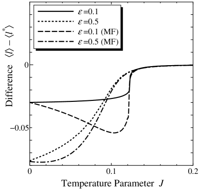
Figure 18: Comparison to the difference $\langle\ell\rangle-\langle\ell^{\ast}\rangle$ estimated by the saddle-point of the mean-field free energy at various densities; $\epsilon=$0.1 (solid and dashed) and 0.5 (dotted and dotted-dashed).

Let us see what comes out if we calculate the Polyakov loop using the ansatz (26) with the solution to Eq. (27) assuming that the second equation of (27) stems from a constraint associated with gauge dynamics. In Fig. 18 we show the difference $\langle\ell\rangle-\langle\ell^{\ast}\rangle$ as a function of $J$. The solid and dotted curves at $\epsilon=0.1$ and $\epsilon=0.5$ respectively are just the same as already presented in Fig. 12. The dashed and dotted-dashed curves are the counterparts derived from the mean-field energy with $x$ and $y$.

In view of two $\epsilon=0.5$ curves, on the one hand, the mean-field result is entirely consistent with what we found in the phase reweighting method. On the other hand, the coincidence is not very good for the $\epsilon=0.1$ results except for $J\simeq 0$ and $J>J_{\text{c}}$. This discrepancy comes from a singularity of the dense-heavy model located at $\epsilon=0$; when $\epsilon$ is small, the fermion action in the dense-heavy model is approximated as $S_{\text{f}}[L]\sim-3\epsilon\sum_{\vec{x}}\ell(\vec{x})$. Hence, nonzero $\epsilon$ tends to align the vacuum into the direction of $x=y$ (see Eq. (26)), and the model does not reduce to a pure gluonic theory with $y=0$ smoothly in the limit of $\epsilon\to 0^{+}$. This situation makes a sharp contrast to finite density QCD. In the strong coupling expansion, for a simple example, the fermion action is $S_{\text{f}}[L]\sim H\sum_{\vec{x}}\bigl{[}\ell(\vec{x})e^{\mu_{q}/T}+\ell^{\ast}(\vec{x})e^{-\mu_{q}/T}\bigr{]}$. In the limit of $\mu_{q}\to 0$, therefore, the fermionic action acts as an external field toward $x\neq 0$ and $y=0$, so that the vacuum alignment of a pure gluonic theory is smoothly retrieved in the $\mu_{q}\to 0$ and $H\to 0^{+}$ limit.

Apart from the discrepancy inherent to the singular behavior of the dense-heavy model near $\epsilon=0$, the mean-field free energy leads to the results in accord with the phase reweighting method. This is an indirect evidence for that the saddle-point is not harmful actually, as we conjectured.

We shall comment on a possible clue to resolve the sign problem based on what we have seen here. We changed the sign problem into a form of the saddle-point of the mean-field free energy. The saddle-point appears harmless from our analyses, presumably stabilized by the Gauss law, and then the sign problem is resolved. Of course, it is highly nontrivial how to map this analytical procedure to the lattice QCD simulation. Still, we would point out that the clustering method developed in Ref. Alford:2001ug is a philosophically similar idea along this line; partial integration over the cluster domains wipes away the sign problem, just like seen in our mean-field free energy free from the sign problem after the group integration.

The field-theoretical approach to reveal the relation between the saddle-point of the free energy and the Gauss law is beyond our current scope, but it definitely deserves further investigation.

IV Summary

We investigated the dense-heavy model and observed the sign problem at finite density within the framework of the mean-field approximation. We calculated the quark number density, the fundamental and adjoint Polyakov loop, the susceptibility, and the phase of the fermion determinant as a function of the model parameters specifying the temperature and the density. All the mean-field results are reasonable and even in quantitative agreement with the lattice data.

In the environment free from the sign problem in the SU(2) case we found that the mean-field approximation goes better than expected. Our mean-field results nicely reproduced the quark number density and the Polyakov loop measured on the lattice once the unknown Polyakov loop renormalization is fixed by fitting. Then, we proceeded into the SU(3) case where the sign problem is relevant.

We saw that the approximation scheme which is capable of describing the different $\mu_{q}$ dependence of $\langle\ell\rangle$ and $\langle\ell^{\ast}\rangle$ cannot avoid the sign problem even at the mean-field level. We applied the phase reweighting method as a practical resolution in order to handle the complex fermion determinant. We acquired $\langle\ell\rangle-\langle\ell^{\ast}\rangle$ as a function of the density parameter or the temperature parameter. So far, there are not many lattice data available for this quantity, but our results $\langle\ell^{\ast}\rangle>\langle\ell\rangle$ are consistent with other model studies as well as what has been obtained from the Taylor expansion method on the lattice.

The important message from our work is the following. The sign problem may be a serious obstacle even in the mean-field model studies at finite temperature and density. We would say, at least, that one should be careful enough when one deals with the Polyakov loop behavior at finite density. The chiral effective models with the Polyakov loop coupled are examples that definitely need more or less caution for application to the finite density problem. The phase reweighting method is one prescription in order to approximate the expectation value in a manageable way. This prescription is, however, only practical and not any solution to the sign problem. We would insist that one cannot solve the QCD sign problem until one can at least find a solution to the sign problem appearing even in that simple model setting. The converse is not necessarily true, though.

In the future, we would like to apply other ideas than the phase reweighting method for the sign problem at the mean-field level. The bottom line here is, thus, that we have formulated an analytical testing ground to think about the sign problem, and we believe that our clarification would be useful for further developments.

- (1) For theoretical reviews on QCD in extreme environments, see, H. Meyer-Ortmanns, Rev. Mod. Phys. 68, 473 (1996) [arXiv:hep-lat/9608098]; F. Wilczek, arXiv:hep-ph/0003183; D. H. Rischke, Prog. Part. Nucl. Phys. 52, 197 (2004) [arXiv:nucl-th/0305030].
- (2) For reviews on recent experimental data and interpretation, see, M. Gyulassy and L. McLerran, Nucl. Phys. A 750, 30 (2005) [arXiv:nucl-th/0405013]; J. L. Nagle, arXiv:nucl-th/0608070.
- (3) For reviews on color superconductivity and the phase diagram of cold and dense quark matter, see, K. Rajagopal and F. Wilczek, arXiv:hep-ph/0011333; K. Fukushima, arXiv:hep-ph/0510299; M. G. Alford, arXiv:hep-lat/0610046; S. B. Ruster, V. Werth, M. Buballa, I. A. Shovkovy and D. H. Rischke, arXiv:nucl-th/0602018.
- (4) For reviews on lattice QCD simulations, see, F. Karsch, Lect. Notes Phys. 583, 209 (2002) [arXiv:hep-lat/0106019]; K. Kanaya, Nucl. Phys. A 715, 233 (2003) [arXiv:hep-ph/0209116]; E. Laermann and O. Philipsen, Ann. Rev. Nucl. Part. Sci. 53, 163 (2003) [arXiv:hep-ph/0303042]; C. Schmidt and T. Umeda, arXiv:hep-lat/0609032.
- (5) M. Cheng et al., Phys. Rev. D 74, 054507 (2006) [arXiv:hep-lat/0608013]; Y. Aoki, Z. Fodor, S. D. Katz and K. K. Szabo, Phys. Lett. B 643, 46 (2006) [arXiv:hep-lat/0609068].
- (6) Y. Aoki, Z. Fodor, S. D. Katz and K. K. Szabo, JHEP 0601, 089 (2006) [arXiv:hep-lat/0510084].
- (7) C. Bernard et al. [MILC Collaboration], Phys. Rev. D 71, 034504 (2005) [arXiv:hep-lat/0405029].
- (8) T. Umeda, K. Nomura and H. Matsufuru, Eur. Phys. J. C 39S1, 9 (2005) [arXiv:hep-lat/0211003]; M. Asakawa and T. Hatsuda, Phys. Rev. Lett. 92, 012001 (2004) [arXiv:hep-lat/0308034]; S. Datta, F. Karsch, P. Petreczky and I. Wetzorke, Phys. Rev. D 69, 094507 (2004) [arXiv:hep-lat/0312037].
- (9) For reviews on the sign problem, see, S. Muroya, A. Nakamura, C. Nonaka and T. Takaishi, Prog. Theor. Phys. 110, 615 (2003) [arXiv:hep-lat/0306031]; M. P. Lombardo, Prog. Theor. Phys. Suppl. 153, 26 (2004) [arXiv:hep-lat/0401021]; S. Aoki, Int. J. Mod. Phys. A 21, 682 (2006) [arXiv:hep-lat/0509068].
- (10) Z. Fodor and S. D. Katz, Phys. Lett. B 534, 87 (2002) [arXiv:hep-lat/0104001]; JHEP 0203, 014 (2002) [arXiv:hep-lat/0106002]; JHEP 0404, 050 (2004) [arXiv:hep-lat/0402006].
- (11) C. R. Allton et al., Phys. Rev. D 66, 074507 (2002) [arXiv:hep-lat/0204010]; C. R. Allton, S. Ejiri, S. J. Hands, O. Kaczmarek, F. Karsch, E. Laermann and C. Schmidt, Phys. Rev. D 68, 014507 (2003) [arXiv:hep-lat/0305007].
- (12) M. G. Alford, A. Kapustin and F. Wilczek, Phys. Rev. D 59, 054502 (1999) [arXiv:hep-lat/9807039]; P. de Forcrand and O. Philipsen, Nucl. Phys. B 642, 290 (2002) [arXiv:hep-lat/0205016]; Nucl. Phys. B 673, 170 (2003) [arXiv:hep-lat/0307020]; [arXiv:hep-lat/0607017]; M. D’Elia and M. P. Lombardo, Phys. Rev. D 67, 014505 (2003) [arXiv:hep-lat/0209146].
- (13) A. M. Polyakov, Phys. Lett. B 72, 477 (1978); L. Susskind, Phys. Rev. D 20, 2610 (1979); B. Svetitsky and L. G. Yaffe, Nucl. Phys. B 210, 423 (1982); B. Svetitsky, Phys. Rept. 132, 1 (1986).
- (14) L. D. McLerran and B. Svetitsky, Phys. Lett. B 98, 195 (1981); L. D. McLerran and B. Svetitsky, Phys. Rev. D 24, 450 (1981); J. Kuti, J. Polonyi and K. Szlachanyi, Phys. Lett. B 98, 199 (1981).
- (15) N. Weiss, Phys. Rev. D 24, 475 (1981); Phys. Rev. D 25, 2667 (1982); V. M. Belyaev, Phys. Lett. B 241, 91 (1990); Phys. Lett. B 254, 153 (1991); C. P. Korthals Altes, Nucl. Phys. B 420, 637 (1994) [arXiv:hep-th/9310195]; K. Fukushima and K. Ohta, J. Phys. G 26, 1397 (2000) [arXiv:hep-ph/0011108];
- (16) J. Polonyi and K. Szlachanyi, Phys. Lett. B 110, 395 (1982); M. Gross, J. Bartholomew and D. Hochberg, “SU(N) Deconfinement Transition And The N State Clock Model,” EFI-83-35-CHICAGO.
- (17) A. Dumitru and R. D. Pisarski, Phys. Lett. B 504, 282 (2001) [arXiv:hep-ph/0010083]; Phys. Lett. B 525, 95 (2002) [arXiv:hep-ph/0106176]; Phys. Rev. D 66, 096003 (2002) [arXiv:hep-ph/0204223].
- (18) A. Gocksch and M. Ogilvie, Phys. Rev. D 31, 877 (1985); K. Fukushima, Phys. Lett. B 553, 38 (2003) [arXiv:hep-ph/0209311]; Phys. Rev. D 68, 045004 (2003) [arXiv:hep-ph/0303225].
- (19) Y. Hatta and K. Fukushima, Phys. Rev. D 69, 097502 (2004) [arXiv:hep-ph/0307068]; A. Mocsy, F. Sannino and K. Tuominen, Phys. Rev. Lett. 92, 182302 (2004) [arXiv:hep-ph/0308135].
- (20) K. Fukushima, Phys. Lett. B 591, 277 (2004) [arXiv:hep-ph/0310121].
- (21) C. P. Korthals Altes, R. D. Pisarski and A. Sinkovics, Phys. Rev. D 61, 056007 (2000) [arXiv:hep-ph/9904305].
- (22) N. Weiss, Phys. Rev. D 35, 2495 (1987).
- (23) E. Megias, E. Ruiz Arriola and L. L. Salcedo, Phys. Rev. D 74, 065005 (2006) [arXiv:hep-ph/0412308]; S. K. Ghosh, T. K. Mukherjee, M. G. Mustafa and R. Ray, Phys. Rev. D 73, 114007 (2006) [arXiv:hep-ph/0603050]; H. Hansen, W. M. Alberico, A. Beraudo, A. Molinari, M. Nardi and C. Ratti, arXiv:hep-ph/0609116; S. Mukherjee, M. G. Mustafa and R. Ray, arXiv:hep-ph/0609249.
- (24) C. Ratti, M. A. Thaler and W. Weise, Phys. Rev. D 73, 014019 (2006) [arXiv:hep-ph/0506234]; S. Roessner, C. Ratti and W. Weise, arXiv:hep-ph/0609281.
- (25) A. Dumitru, R. D. Pisarski and D. Zschiesche, Phys. Rev. D 72, 065008 (2005) [arXiv:hep-ph/0505256].
- (26) T. C. Blum, J. E. Hetrick and D. Toussaint, Phys. Rev. Lett. 76, 1019 (1996) [arXiv:hep-lat/9509002]. (We note that the published version of this paper does not contain the SU(2) results which are present in the preprint version. We refer only to the preprint version.)
- (27) I. Bender et al., Nucl. Phys. Proc. Suppl. 26, 323 (1992); J. Engels, O. Kaczmarek, F. Karsch and E. Laermann, Nucl. Phys. B 558, 307 (1999) [arXiv:hep-lat/9903030].
- (28) D. T. Son and M. A. Stephanov, Phys. Rev. Lett. 86, 592 (2001) [arXiv:hep-ph/0005225].
- (29) E. Dagotto, F. Karsch and A. Moreo, Phys. Lett. B 169, 421 (1986); J. U. Klatke and K. H. Mutter, Nucl. Phys. B 342, 764 (1990); S. Hands, J. B. Kogut, M. P. Lombardo and S. E. Morrison, Nucl. Phys. B 558, 327 (1999) [arXiv:hep-lat/9902034]; J. B. Kogut, D. Toublan and D. K. Sinclair, Phys. Lett. B 514, 77 (2001) [arXiv:hep-lat/0104010]; J. B. Kogut, D. Toublan and D. K. Sinclair, Nucl. Phys. B 642, 181 (2002) [arXiv:hep-lat/0205019]; J. B. Kogut, D. Toublan and D. K. Sinclair, Phys. Rev. D 68, 054507 (2003) [arXiv:hep-lat/0305003]; S. Muroya, A. Nakamura and C. Nonaka, Phys. Lett. B 551, 305 (2003) [arXiv:hep-lat/0211010]; B. Vanderheyden and A. D. Jackson, Phys. Rev. D 64, 074016 (2001) [arXiv:hep-ph/0102064]; J. B. Kogut, M. A. Stephanov and D. Toublan, Phys. Lett. B 464, 183 (1999) [arXiv:hep-ph/9906346]; J. B. Kogut, M. A. Stephanov, D. Toublan, J. J. M. Verbaarschot and A. Zhitnitsky, Nucl. Phys. B 582, 477 (2000) [arXiv:hep-ph/0001171]; Y. Nishida, K. Fukushima and T. Hatsuda, Phys. Rept. 398, 281 (2004) [arXiv:hep-ph/0306066]; S. Chandrasekharan and F. J. Jiang, Phys. Rev. D 74, 014506 (2006) [arXiv:hep-lat/0602031]; B. Alles, M. D’Elia and M. P. Lombardo, Nucl. Phys. B 752, 124 (2006) [arXiv:hep-lat/0602022]; S. Hands, S. Kim and J. I. Skullerud, arXiv:hep-lat/0604004.
- (30) P. Hasenfratz and F. Karsch, Phys. Rept. 103, 219 (1984).
- (31) J. B. Kogut, M. Snow and M. Stone, Nucl. Phys. B 200, 211 (1982).
- (32) J. Engels, J. Fingberg and M. Weber, Nucl. Phys. B 332, 737 (1990).
- (33) A. Dumitru, Y. Hatta, J. Lenaghan, K. Orginos and R. D. Pisarski, Phys. Rev. D 70, 034511 (2004) [arXiv:hep-th/0311223].
- (34) F. Lenz and M. Thies, Annals Phys. 268, 308 (1998) [arXiv:hep-th/9802066].
- (35) P. de Forcrand and V. Laliena, Phys. Rev. D 61, 034502 (2000) [arXiv:hep-lat/9907004].
- (36) M. Oleszczuk and J. Polonyi, Annals Phys. 227, 76 (1993).
- (37) A. Barducci, R. Casalbuoni, S. De Curtis, R. Gatto and G. Pettini, Phys. Lett. B 231, 463 (1989); F. Wilczek, Int. J. Mod. Phys. A 7, 3911 (1992) [Erratum-ibid. A 7, 6951 (1992)]; A. Barducci, R. Casalbuoni, G. Pettini and R. Gatto, Phys. Rev. D 49, 426 (1994); J. Berges and K. Rajagopal, Nucl. Phys. B 538, 215 (1999) [arXiv:hep-ph/9804233]; M. A. Halasz, A. D. Jackson, R. E. Shrock, M. A. Stephanov and J. J. M. Verbaarschot, Phys. Rev. D 58, 096007 (1998) [arXiv:hep-ph/9804290]; M. A. Stephanov, K. Rajagopal and E. V. Shuryak, Phys. Rev. Lett. 81, 4816 (1998) [arXiv:hep-ph/9806219]; M. A. Stephanov, K. Rajagopal and E. V. Shuryak, Phys. Rev. D 60, 114028 (1999) [arXiv:hep-ph/9903292]; K. Fukushima, Phys. Rev. C 67, 025203 (2003) [arXiv:hep-ph/0209270]; Y. Hatta and T. Ikeda, Phys. Rev. D 67, 014028 (2003) [arXiv:hep-ph/0210284].
- (38) M. Asakawa and K. Yazaki, Nucl. Phys. A 504, 668 (1989);
- (39) M. G. Alford, S. Chandrasekharan, J. Cox and U. J. Wiese, Nucl. Phys. B 602, 61 (2001) [arXiv:hep-lat/0101012].
- (40) S. Kim, Ph. de Forcrand, S. Kratochvila and T. Takaishi, PoS LAT2005, 166 (2006) [arXiv:hep-lat/0510069].