An approach to NNLO QCD analysis of non-singlet structure function

Abstract

We use the next-to-next-to-leading order (NNLO) contributions to anomalous dimension governing the evolution of non-singlet quark distributions. We use the $xF_{3}$ data of the CCFR collaboration to obtain some unknown parameters which exist in the non-singlet quark distributions in the NNLO approximation. In the fitting procedure, Bernstein polynomial method is used. The results of valence quark distributions in the NNLO, are in good agreement with the available theoretical model.

I Introduction

The global parton analyses of deep inelastic scattering (DIS) and the related hard scattering data are generally performed at NLO order. Presently the next-to leading order (NLO) is the standard approximation for most important processes in QCD.

The corresponding one- and two-loop splitting functions have been known for a long time Gross:1973rr ; Georgi:1974sr ; Altarelli:1977zs ; Floratos:1977au ; Floratos:1979ny ; Gonzalez-Arroyo:1979df ; Gonzalez-Arroyo:1980he ; Curci:1980uw ; Furmanski:1980cm ; Floratos:1981hs ; Hamberg:1992qt . The NNLO corrections should to be included in order to arrive at quantitatively reliable predictions for hard processes occurring at present and future high-energy colliders. These corrections are so far known only for the structure functions in the deep-inelastic scattering vanNeerven:1991nn ; Zijlstra:1991qc ; Zijlstra:1992kj ; Zijlstra:1992qd .

Recently much effort has been invested in computing NNLO QCD corrections to a wide variety of partonic processes and therefore it is needed to generate parton distributions also at NNLO so that the theory can be applied in a consistent manner.

S. Moch and et al. Moch:2004pa ; Vogt:2004ns computed the higher order contributions up to three-loops splitting functions governing the evolution of unpolarized non-singlet quark densities in perturbative QCD.

During the recent years the interest to use CCFR data CCFR:1997 for $xF_{3}$ structure function in higher orders, based on orthogonal polynomial expansion method has been increased Kataev:1997nc ; Kataev:1998ce ; Alekhin:1998df ; Kataev:1999bp ; Kataev:2001kk ; Santiago:2001mh .

In this paper we determine the flavor non-singlet parton distribution functions, $xu_{v}(x,Q^{2})$ and $xd_{v}(x,Q^{2})$, using the Bernstein polynomial approach up to NNLO level. This calculation is possible now, as the non-singlet anomalous dimensions in $n$-Moment space in three loops have been already introduced Moch:2004pa ; Vogt:2004ns .

II The theoretical background of the QCD analysis

In the NNLO approximation the deep inelastic coefficient functions are known and also the anomalous dimensions in $n$-Moment space are available at this orderMoch:2004pa ; Vogt:2004ns . Since in this paper we want to calculate the non-singlet parton distribution functions in the NNLO by using CCFR experimental data, we introduce the moments of non-singlet structure function up to three loops order.

Let us define the Mellin moments for the $\nu$N structure function $xF_{3}(x,Q^{2})$:

$${\cal{M}}_{n}(Q^{2})=\int_{0}^{1}x^{n-1}F_{3}(x,Q^{2})dx\;.$$ (1)

The theoretical expression for these moments obey the following renormalization group equation

$$\bigg{(}\mu\frac{\partial}{\partial\mu}+\beta(A_{s})\frac{\partial}{\partial A_{s}}+\gamma_{NS}^{(n)}(A_{s})\bigg{)}{\cal{M}}_{n}(Q^{2}/\mu^{2},A_{s}(\mu^{2}))=0\;,$$ (2)

where $A_{s}=\alpha_{s}/(4\pi)$ is the renormalization group coupling and is governed by the QCD $\beta$-function as

$$\mu\frac{\partial A_{s}}{\partial\mu}=\beta(A_{s})=-2\sum_{i\geq 0}\beta_{i}A_{s}^{i+2}\;.$$ (3)

The solution of Eq.(3) in the NNLO is given by

$$A_{s}^{NNLO} = \frac{1}{\beta_{0}\ln Q^{2}/\Lambda_{\overline{MS}}^{2}}-\frac{\beta_{1}\ln(\ln Q^{2}/\Lambda_{\overline{MS}}^{2})}{\beta_{0}^{3}(\ln Q^{2}/\Lambda_{\overline{MS}}^{2})^{2}}+$$

$$\frac{1}{\beta_{0}^{5}(\ln Q^{2}/\Lambda_{\overline{MS}}^{2})^{3}}[\beta_{1}^{2}\ln^{2}(\ln Q^{2}/\Lambda_{\overline{MS}}^{2})-$$

$$\beta_{1}^{2}\ln(\ln Q^{2}/\Lambda_{\overline{MS}}^{2})+\beta_{2}\beta_{0}-\beta_{1}^{2}]\;.$$

Notice that in the above the numerical expressions for $\beta_{0}$, $\beta_{1}$ and $\beta_{2}$ are

$$\beta_{0} = 11-0.6667f\;,$$

$$\beta_{1} = 102-12.6667f\;,$$

$$\beta_{2} = 1428.50-279.611f+6.01852f^{2}\;,$$ (5)

where $f$ denotes the number of active flavors.

The solution of the renormalization group equation for non-singlet structure function $xF_{3}$ can be presented in the following form Kataev:1999bp :

$$\frac{{\cal{M}}_{n}(Q^{2})}{{\cal{M}}_{n}(Q_{0}^{2})}=exp\bigg{[}-\int_{A_{s}(Q_{0}^{2})}^{A_{s}(Q^{2})}\frac{\gamma_{NS}^{(n)}(x)}{\beta(x)}dx\bigg{]}\frac{C_{NS}^{(n)}(A_{s}(Q^{2}))}{C_{NS}^{(n)}(A_{s}(Q_{0}^{2}))}\;,$$ (6)

where ${\cal{M}}_{n}(Q_{0}^{2})$ is a phenomenological quantity related to the factorization scale dependent factor which we will parameterize in next section. $\gamma_{n}^{NS}$ is the anomalous function and has a perturbative expansion as

$$\gamma_{n}^{NS}(A_{s})=\sum_{i\geq 0}\gamma_{i}^{NS}(n)A_{s}^{i+1}\;.$$ (7)

At the NNLO the expression for the coefficient function $C^{(n)}_{NS}$ can be presented as Moch:1999eb

$$C_{NS}^{(n)}(A_{s})=1+C^{(1)}(n)A_{s}+C^{(2)}(n)A_{s}^{2}\;.$$ (8)

With the corresponding expansion of the anomalous dimensions, given by Eq. (7), the solution to the three loops evolution equation from Eq. (6), is as follows

$${\cal{M}}_{n}^{NNLO}(Q^{2})=\left(\frac{A_{s}(Q^{2})}{A_{s}(Q_{0}^{2})}\right)^{\gamma_{0}^{NS}/2\beta_{0}}\times$$

$$\left\{1+[A_{s}(Q^{2})-A_{s}(Q_{0}^{2})]\left(\frac{\gamma_{1}}{2\beta_{1}}-\frac{\gamma_{0}^{NS}}{2\beta_{0}}\right)\frac{\beta_{1}}{\beta_{0}}\right.$$

$$+[A_{s}(Q^{2})-A_{s}(Q_{0}^{2})]^{2}\frac{\beta_{1}^{2}}{8\beta_{0}^{2}}\left(\frac{\gamma_{1}}{\beta_{1}}-\frac{\gamma_{0}^{NS}}{\beta_{0}}\right)^{2}$$

$$+\frac{1}{4}[A_{s}^{2}(Q^{2})-A_{s}^{2}(Q_{0}^{2})]$$

$$\left.\left(\frac{1}{\beta_{0}}\gamma_{2}-\frac{\beta_{1}}{\beta_{0}^{2}}\gamma_{1}+\frac{\beta_{1}^{2}-\beta_{2}\beta_{0}}{\beta_{0}^{3}}\gamma_{0}^{NS}\right)\right\}$$

$$\left(1+C^{(1)}A_{s}(Q^{2})+C^{(2)}A_{s}^{2}(Q^{2})\right)V(n,Q_{0}^{2})\;.$$ (9)

Where $V$ is the valence quark compositions as

$$V(n,Q_{0}^{2})=u_{v}(n,Q_{0}^{2})+d_{v}(n,Q_{0}^{2})\;.$$ (10)

As we see in Mellin-$n$ space the non-singlet (NS) parts of structure function in the NNLO approximation for example, i.e.$\;{\cal{M}}_{n}^{NNLO}(Q^{2})$, can be obtained from the corresponding Wilson coefficients $C^{(k)}$ and the non-singlet quark densities.

In next section we will introduce the functional form of the valence quark distributions and we will parameterize these distributions at the scale of $Q_{0}^{2}$.

By using the anomalous dimensions in one , two and three loops from Moch:2004pa and inserting them in Eq. (II), the moment of non-singlet structure function in the NNLO as a function of $n$ and $Q^{2}$ is available.

III Parametrization of the parton densities

In this section we will discuss how we can determine the parton distribution at the input scale of $Q_{0}^{2}=1$ GeV². To start the parameterizations of the above mentioned parton distributions at the input scale of $Q_{0}^{2}$ we assume the following functional form

$$xu_{v}(x,Q_{0}^{2})=N_{u}x^{a}(1-x)^{b}(1+c\sqrt{x}+dx)\;,$$ (11)

$$xd_{v}(x,Q_{0}^{2})=\frac{N_{d}}{N_{u}}(1-x)^{e}\;xu_{v}(x,Q_{0}^{2})\;.$$ (12)

In the above the $x^{a}$ term controls the low-$x$ behavior parton densities, and $(1-x)^{b,e}$ large values of $x$. The remaining polynomial factor accounts for additional medium-$x$ values. Normalization constants $N_{u}$ and $N_{d}$ are fixed by

$$\int_{0}^{1}u_{v}(x)dx=2\;,$$ (13)

$$\int_{0}^{1}d_{v}(x)dx=1\;.$$ (14)

The above normalizations are very effective to control unknown parameters in Eqs. (11,12) via the fitting procedure. The five parameters with $\Lambda_{QCD}^{N_{f}=4}$ will be extracted by using the Bernstain polynomials approach.

Using the valence quark distribution functions, the moments of $u_{v}(x,Q_{0}^{2})$ and $d_{v}(x,Q_{0}^{2})$ distributions can be easily calculated. Now by inserting the Mellin moments of $u_{v}$ and $d_{v}$ valence quark in the Eq. (10), the function of $V(n,Q_{0}^{2})$ involves some unknown parameters.

IV Averaged structure functions

Although it is relatively easy to compute the $n$th moment from the structure functions, the inverse process is not obvious. To do this inversion, we adopt a mathematically rigorous but easy method Yndu:78 to invert the moments and retrieve the structure functions. The method is based on the fact that for a given value of $Q^{2}$, only a limited number of experimental points, covering a partial range of values of $x$ are available. The method devised to deal with this situation is to take averages of the structure function weighted by suitable polynomials. These are the Bernstein polynomials which are defined by

$$B_{nk}(x)=\frac{\Gamma(n+2)}{\Gamma(k+1)\Gamma(n-k+1)}x^{k}(1-x)^{n-k}\;;\;n\geq{k}\;.$$ (15)

Using the binomial expansion, the above equation can be written as

$$B_{n,\;k}(x)=\frac{\Gamma(n+2)}{\Gamma(k+1)}\sum_{l=0}^{n-k}\frac{(-1)^{l}}{l!(n-k-l)!}\;x^{k+l}\;.$$ (16)

Now, we can compare theoretical predictions with the experimental results for the Bernstein averages, which are given by Max:2002 ; KAM:2004

$$F_{nk}(Q^{2}){\equiv}\int_{0}^{1}dxB_{nk}(x)F_{3}(x,Q^{2})\;.$$ (17)

Therefore, the integral Eq. (17) represents an average of the function $F_{3}(x,Q^{2})$ in the region ${\bar{x}}_{nk}-\frac{1}{2}\Delta{x}_{nk}{\leq}x{\leq}{\bar{x}}_{n,k}+\frac{1}{2}\Delta{x}_{nk}$. The key point is, the values of $F_{3}$ outside this interval have a small contribution to the above integral, as $B_{nk}(x)$ tends to zero very quickly. In order to ensure the equivalence of the integral Eq. (17) to the same integral in the range $x_{1}={\bar{x}}_{nk}-\frac{1}{2}\Delta{x}_{nk}$ to $x_{2}={\bar{x}}_{nk}+\frac{1}{2}\Delta{x}_{nk}$, we have to use the normalization factor, $\int_{x_{1}}^{x_{2}}dxB_{nk}(x)$ in the denominator of Eq. (17) which obviously is not equal to $1$. So it can be written:

$$F_{nk}(Q^{2}){\equiv}\frac{\int_{{\bar{x}}_{nk}-\frac{1}{2}\Delta{x}_{nk}}^{{\bar{x}}_{nk}+\frac{1}{2}\Delta{x}_{nk}}\;dx\;B_{nk}(x)\;F_{3}(x,Q^{2})}{\int_{{\bar{x}}_{nk}-\frac{1}{2}\Delta{x}_{nk}}^{{\bar{x}}_{nk}+\frac{1}{2}\Delta{x}_{nk}}\;dx\;B_{nk}(x)}\;.$$ (18)

By a suitable choice of $n$, $k$ we manage to adjust to the region where the average is peaked around values which we have experimental data CCFR:1997 .

Substituting Eq. (16) in Eq. (17), it follows that the averages of $F_{3}$ with $B_{nk}(x)$ as weight functions can be obtained in terms of odd and even moments,

$$F_{nk} = \frac{{(n-k)!}{\Gamma(n+2)}}{\Gamma(k+1)\Gamma(n-k+1)}\times$$

$$\sum_{l=0}^{n-k}\frac{(-1)^{l}}{l!(n-k-l)!}\;{{\cal{M}}({(k+l)+1}},Q^{2})\;.$$

We can only include a Bernstein average, $F_{nk}$, if we have experimental points covering the whole range [${\bar{x}}_{nk}-\frac{1}{2}\Delta{x}_{nk},{\bar{x}}_{nk}+\frac{1}{2}\Delta{x}_{nk}$] SantYun . This means that with the available experimental data we can only use the following 28 averages, including

$F_{2,1}^{(\exp)}(Q^{2}),F_{3,1}^{(\exp)}(Q^{2}),F_{4,2}^{(\exp)}(Q^{2})$,…, $F_{13,4}^{(\exp)}(Q^{2})$.

Another restriction we assume here, is to ignore the effects of moments with high order $n$ which do not strongly constrain the fits. To obtain these experimental averages from CCFR data CCFR:1997 , we fit $x{F_{3}}(x,{Q^{2}})$ for each bin in ${Q}^{2}$ separately to the convenient phenomenological expression

$${xF_{3}}^{{(phen)}}={\cal{A}}x^{\cal{B}}(1-x)^{\cal{C}}\;.$$ (20)

This form ensures zero values for ${xF_{3}}$ at $x=0$, and $x=1$. In Table 1 we have presented the numerical values of $\cal{A},\cal{B}$ and $\cal{C}$ at $Q^{2}=20,31.6,50.1,79.4,125.9$ GeV².

$Q^{2}(GeV^{2})$	$\mathcal{A}$	$\mathcal{B}$	$\mathcal{C}$
$20$	$4.742$	$0.636$	$3.376$
$31.6$	$5.473$	$0.694$	$3.659$
$50.1$	$5.679$	$0.698$	$3.839$
$79.4$	$4.508$	$0.567$	$3.757$
$125.9$	$7.077$	$0.819$	$4.246$

Table 1: Numerical values of fitting ${\cal{A}},{\cal{B}},{\cal{C}}$ parameters in Eq. (20).

Using Eq. (20) with the fitted values of ${\cal{A}},{\cal{B}}$ and ${\cal{C}}$, one can then compute ${F}_{nk}^{(exp)}({Q}^{2})$ in terms of Gamma functions. Some sample experimental Bernstein averages are plotted in Fig. 1 in the higher approximations. The errors in the ${F}_{nk}^{(exp)}(Q^{2})$ correspond to allowing the CCFR data for $x{F}_{3}$ to vary within the experimental error bars, including the experimental systematic and statistical errors CCFR:1997 . We have only included data for ${Q}^{2}{\geq}20{\rm{GeV}}^{2}$, this has the merit of simplifying the analysis by avoiding evolution through flavor thresholds.

Using Eq. (LABEL:eq:FnkExpandMOM), the 28 Bernstein averages ${F}_{nk}({Q}^{2})$ can be written in terms of odd and even moments. For instance:

$${F_{2,1}}(Q^{2})=6\left({\cal{M}}(2,Q^{2})-{\cal{M}}(3,Q^{2})\right)\;,$$

$$\vdots$$ (21)

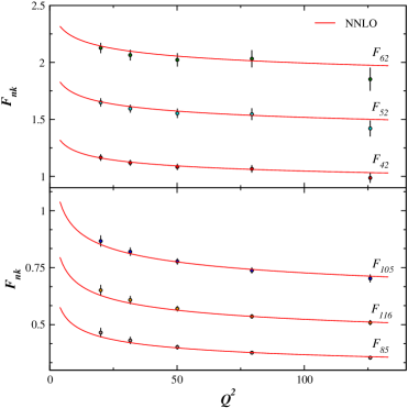
Figure 1: NNLO fit to Bernstein averages of $xF_{3}$.

The unknown parameters according to Eqs. (11,12) will be $a,b,c,d,e$ and $\Lambda_{QCD}^{N_{f}}$. Thus, there are 6 parameters for each order to be simultaneously fitted to the experimental ${F}_{nk}({Q}^{2})$ averages. Using the CERN subroutine MINUIT MINUIT:CERN , we defined a global ${\chi}^{2}$ for all the experimental data points and found an acceptable fit with minimum ${\chi}^{2}/{\rm{dof}}=74.772/134=0.558$ in the NNLO case with the standard error of order $10^{-3}$. The best fit is indicated by some sample curves in the Fig. 1. The fitting parameters and the minimum ${\chi}^{2}$ values in each order are listed in Table 2.

From Eqs.(11,12), we are able now to determine the $xu_{v}$ and $xd_{v}$ at the scale of $Q_{0}^{2}$ in higher order corrections. In Fig. 2 we have plotted the NLO and NNLO approximation results of $xu_{v}$ and $xd_{v}$ at the input scale $Q_{0}^{2}=1.0\;GeV^{2}$ (solid line) compared to the results obtained from NNLO analysis (left panels) and NLO analysis (right panels) by MRST (dashed-dotted line) Martin:2004 and A05(dashed line)Alekhin:2005gq .

	NNLO
$N_{u}$	5.134
$a$	0.830
$b$	3.724
$c$	0.040
$d$	1.449
$N_{d}$	3.348
$e$	1.460
$\Lambda_{QCD}^{(4)},MeV$	230
$\chi^{2}/$ndf	0.558

Table 2: Parameter values of the NNLO non-singlet QCD fit at $Q_{0}^{2}=1$ GeV².

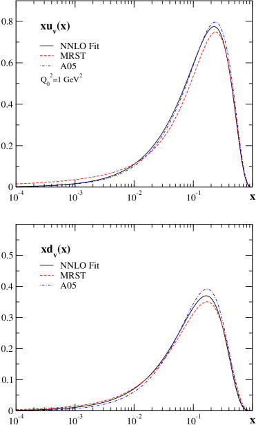
Figure 2: The parton densities $xu_{v}$ and $xd_{v}$ at the input scale $Q_{0}^{2}=1.0\;GeV^{2}$ (solid line) compared to results obtained from NNLO analysis by MRST (dashed line) Martin:2004 and A05(dashed-dotted line)Alekhin:2005gq .

All of the non-singlet parton distribution functions in moment space for any order are now available, so we can use the inverse Mellin technics to obtain the $Q^{2}$ evolution of valance quark distributions which will be done in the next section.

V $\bf x$ dependent of valence quark densities

In the previous section we parameterized the non-singlet parton distribution functions at input scale of $Q_{0}^{2}=1$ GeV² in the NNLO approximations by using Bernstein averages method. To obtain the non-singlet parton distribution functions in $x$-space and for $Q^{2}>Q_{0}^{2}$ GeV² we need to use the $Q^{2}$-evolution in $n$-space. To obtain the $x$-dependence of parton distributions from the $n-$dependent exact analytical solutions in the Mellin-moment space, one has to perform a numerical integral in order to invert the Mellin-transformation Graudenz:1995sk

$$f^{k}(x,Q^{2}) = \frac{1}{\pi}\int_{0}^{\infty}dw\times$$

$$Im[e^{i\phi}x^{-c-we^{i\phi}}M_{k}(n=c+we^{i\phi},Q^{2})]\;,$$

where the contour of the integration lies on the right of all singularities of $M_{k}(n=c+we^{i\phi},Q^{2})$ in the complex $n$-plane. For all practical purposes one may choose $c\simeq 1,\phi=135^{\circ}$ and an upper limit of integration, for any $Q^{2}$, of about $5+10/\ln x^{-1}$, instead of $\infty$, which guarantees stable numerical results GRV:90 ; GRV:92 .

VI Conclusion

The QCD analysis is performed in NNLO based on Bernstein polynomial approach. We determine the valence quark densities in a wide range of $x$ and $Q^{2}$. Inserting the functions of $q_{v}(n,Q^{2})$ for $q=u,d$ in Eq. (22) we can obtain all valence distribution functions in fixed $Q^{2}$ and in $x$-space. In Fig. 3 we have presented the parton distribution $xu_{v}$ at some different values of $Q^{2}$. These distributions were compared with some theoretical models Martin:2004 ; Alekhin:2005gq .
In Fig. 3 we have also presented the same distributions for $xd_{v}$.

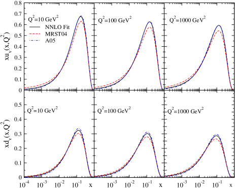
Figure 3: The parton distribution $xu_{v}$ and $xd_{v}$ at some different values of $Q^{2}$. The solid line is our model, dashed line is the MRST model Martin:2004 , dashed-dotted line is the model from Alekhin:2005gq .

The QCD scale $\Lambda_{\rm QCD}^{\rm N_{f}=4}$ is determined together with the parameters of the parton distributions. In our fit results the value of $\Lambda_{\rm QCD}^{\rm N_{f}=4}$ and $\alpha_{s}(M_{Z}^{2})$ at the NNLO analysis is $230$ MeV and $0.1142$ respectively.
Complete details of this paper with calculation of LO, NLO and NNLO and also comparing them with together is reported in Ref. [36].

VII Acknowledgments

We are grateful to A. Mirjalili for useful suggestions and discussions. A.N.K acknowledge to Semnan university for the financial support of this project.

References

- (1) D.J. Gross and F. Wilczek, Phys. Rev. D8 (1973) 3633.
- (2) H. Georgi and H.D. Politzer, Phys. Rev. D9 (1974) 416.
- (3) G. Altarelli and G. Parisi, Nucl. Phys. B126 (1977) 298.
- (4) E.G. Floratos, D.A. Ross and C.T. Sachrajda, Nucl. Phys. B129 (1977) 66.
- (5) E.G. Floratos, D.A. Ross and C.T. Sachrajda, Nucl. Phys. B152 (1979) 493.
- (6) A. Gonzalez-Arroyo, C. Lopez and F.J. Yndurain, Nucl. Phys. B153 (1979) 161.
- (7) A. Gonzalez-Arroyo and C. Lopez, Nucl. Phys. B166 (1980) 429.
- (8) G. Curci, W. Furmanski and R. Petronzio, Nucl. Phys. B175 (1980) 27.
- (9) W. Furmanski and R. Petronzio, Phys. Lett. 97B (1980) 437.
- (10) E.G. Floratos, C. Kounnas and R. Lacaze, Nucl. Phys. B192 (1981) 417.
- (11) R. Hamberg and W.L. van Neerven, Nucl. Phys. B379 (1992) 143.
- (12) W.L. van Neerven and E.B. Zijlstra, Phys. Lett. B272 (1991) 127.
- (13) E.B. Zijlstra and W.L. van Neerven, Phys. Lett. B273 (1991) 476.
- (14) E.B. Zijlstra and W.L. van Neerven, Phys. Lett. B297 (1992) 377.
- (15) E.B. Zijlstra and W.L. van Neerven, Nucl. Phys. B383 (1992) 525.
- (16) S. Moch, J. A. M. Vermaseren and A. Vogt, Nucl. Phys. B 688 (2004) 101.
- (17) A. Vogt, Comput. Phys. Commun. 170, (2005) 65.
- (18) W. G. Seligman et al., Phys. Rev. Lett. 79, (1997) 1213.
- (19) A. L. Kataev, A. V. Kotikov, G. Parente and A. V. Sidorov, Phys. Lett. B 417, (1998) 374.
- (20) A. L. Kataev, G. Parente and A. V. Sidorov, arXiv:hep-ph/9809500.
- (21) S. I. Alekhin and A. L. Kataev, Phys. Lett. B 452, (1999) 402.
- (22) A. L. Kataev, G. Parente and A. V. Sidorov, Nucl. Phys. B 573, (2000) 405.
- (23) A. L. Kataev, G. Parente and A. V. Sidorov, Phys. Part. Nucl. 34, (2003) 20; A. L. Kataev, G. Parente and A. V. Sidorov, Nucl. Phys. Proc. Suppl. 116 (2003) 105.
- (24) J. Santiago and F. J. Yndurain, Nucl. Phys. B 611, (2001) 447.
- (25) S. Moch and J. A. M. Vermaseren, Nucl. Phys. B 573, (2000) 853.
- (26) F. J. Yndurain, Phys. Lett. B 74 (1978) 68.
- (27) C. J. Maxwell and A. Mirjalili, Nucl. Phys. B 645 (2002) 298.
- (28) Ali N. Khorramian, A. Mirjalili, S. Atashbar Tehrani, JHEP10, 062 (2004).
- (29) J. Santiago and F. J. Yndurain, Nucl. Phys. B 563 (1999) 45 ; J. Santiago and F. J. Yndurain, Nucl. Phys. B 611 (2001) 447
- (30) F. James, CERN Program Library Long Writeup D506.
- (31) A. D. Martin, R. G. Roberts, W. J. Stirling and R. S. Thorne, Phys. Lett. B 604, (2004) 61
- (32) S. Alekhin, JETP Lett. 82, 628 (2005) ; S. Alekhin, Phys. Rev. D 68 (2003) 014002.
- (33) D. Graudenz, M. Hampel, A. Vogt and C. Berger, Z. Phys. C 70, (1996) 77
- (34) M. Gluck, E. Reya and A. Vogt, Z. Phys. C 48 (1990) 471.
- (35) M. Gluck, E. Reya and A. Vogt, Phys. Rev. D 45 (1992) 3986.
- (36) Ali N. Khorramian, S. Atashbar Tehrani, hep-ph/0610136.